

Submitted:
30 October 2026
Posted:
02 November 2026
You are already at the latest version
Abstract
Background: Mexico reports collecting 64% of its PET bottles against targets of 70% (2025) and 80% (2030), and informal collectors carry much of that work. A deposit-refund system (DRS) could raise recovery but could also take material and income from them; Mexico’s 2026 Circular Economy Law recognizes base recyclers but creates no DRS. Methods: We build a stock-and-flow model of containers, consumer returns and collector entry and exit, anchor inputs to Mexican sources where they exist, and add a calculation of collector income from six quarters of the national ENOE employment survey. Results: Across simulated systems, a 1.5 MXN deposit with collectors receiving 30% of it on the containers they hand in reaches 80% recovery while keeping at least 90% of collectors in 68–95% of systems, the upper end assuming an optimistic reading of collector income; a 3.0 MXN deposit reaches 92–99%. Failures are almost always consumer-response failures; displacement appears when collector access is low. Consumer hassle cost, collector income margin, entry sensitivity and the accessible share of discards drive most of the uncertainty. Conclusions: A pilot should measure consumer returns at three or more deposit levels, collector access and income, and audited recovery, with decision thresholds we derive.
Keywords:
deposit-refund system
; PET bottles
; informal collectors
; Mexico
; system dynamics
; pilot design
1. Introduction
Mexico’s PET bottle collection rate was reported by the industry association ECOCE as 64% in 2024, equal to 578 thousand tonnes against an apparent consumption of 860 thousand tonnes (ECOCE, 2024, p. 1). The industry’s voluntary National Agreement set collection targets of 70% for PET in 2025 and 80% in 2030 (Acuerdo Nacional, 2023, p. 3). Bottle recovery in Mexico has long depended on informal collectors: an analysis of the national PET recycling system described collection as “in the hands of the informal sector” (Schwanse, 2011, p. 977).
Policy is moving. The General Circular Economy Law published in the Diario Oficial de la Federación on 19 January 2026 defines the “persona recicladora de base o pepenadora” (art. 3, section XXIII) and inclusive recycling (section XXVIII), and instructs authorities to promote it (arts. 21 X and 22 VII) (DOF, 2026, pp. 1, 4, 13, 14). A search of the full published text found no deposit-refund system and no PET-specific target, so a DRS for Mexico is a policy that could be adopted, not one that exists. Any pilot would therefore be designed under the legal expectation that collectors are included, not displaced.
That is the practical problem this paper addresses. A deposit pulls bottles toward consumer returns and away from the mixed waste stream where collectors find them. If consumers return enough, recovery rises; if collectors lose their supply and leave, the informal work that currently delivers much of the recovery may shrink, with social costs for people whose earnings are already low. The design levers are the deposit level D and the share θ of the deposit that collectors receive on the containers they hand in. The uncertainty is large because Mexico has no deposit system for PET from which to read consumer behavior (the only Mexican evidence we found on how consumers respond to a deposit is a 2002 stated-preference survey, Section 2.1), and systematic information on collector earnings and entry is thin.
We do not attempt to forecast what a Mexican DRS would achieve. We use a model to answer two practical questions: which minimal designs (D, θ) could reach 70–80% recovery without displacing collectors under the range of plausible inputs, and which few quantities a pilot must measure to narrow that range fast enough to decide whether to scale. This framing reflects a practical point: results that are conditional on many assumed inputs help a decision only if they identify which inputs, once measured, would change it.
The study follows a companion study of adaptive incentive governance for PET and returnable-glass recovery in Mexico (Madrid Rico, 2026). That study found a composite return-rate ceiling of about 0.759 under its calibrated behavioral response, 2.1 percentage points below the 0.78 composite target (Madrid Rico, 2026, p. 1), and it represented the informal collection network as a single collection-rate parameter, listing an endogenous representation of that network among its future work (Madrid Rico, 2026, p. 12). The present paper addresses that second point with a separate, smaller model in which collectors enter and leave according to their income; it does not reuse the companion model.
The paper makes three contributions. First, a compact model (Section 2.3) with 15 uncertain inputs, of which a global sensitivity analysis shows that only four matter for the decision (Section 3.3). Second, an evidence table (Section 2.1) that states, for every input, whether it is anchored in a Mexican source with a page reference, partly anchored, or an explicit scenario; it includes a new calculation of collector income and of the income margin κ from ENOE microdata. Third, a short list of pilot measurements with decision thresholds derived from the model (Section 4.1).
1.1. Related Work, Briefly
Reviews of deposit-refund systems report return rates that depend strongly on deposit size across jurisdictions: the review’s examples associate a 5-cent deposit in New York and Massachusetts with returns of about 65% and a 10-cent deposit in Michigan with about 95% (Zhou et al., 2020, p. 7), and the review lists the integration of informal enterprises, by hiring or rewarding informal recyclers, among the trends it identifies (Zhou et al., 2020, pp. 1, 9). A critical review of DRS for plastic beverage bottles concludes that designing DRS with attention to social impacts should be a priority and notes that DRS can support the livelihoods of disadvantaged people (Picuno et al., 2025, pp. 7, 9). A simulation of PET bottle recycling in China combines a DRS with recycled-content and tax-refund instruments and represents informal collection as a flow drawn from discards (Wang et al., 2020, pp. 1, 4). Models in which informal workers enter or leave according to their earnings exist for other settings: an agent-based model of plastic packaging in Lima in which collectors enter or exit depending on collection performance but which contains no deposit (Carbonel et al., 2026, p. 5), and a system dynamics model of electronic-waste recycling in which informal workers are hired and laid off according to cash availability (Ardi and Leisten, 2016, pp. 6, 9). An early dynamic model with waste-pickers discusses the deposit-refund as transferring the incentive to the agent with the lowest opportunity cost of time (Moreno-Sánchez and Maldonado, 2006, p. 384). For Mexico, a recent assessment of plastics circularity stresses that the transferability of designs from other countries is conditional (Carmona-Estrada et al., 2026, p. 9). Our model uses the entry-exit idea of Carbonel et al. (2026) and Ardi and Leisten (2016) together with a consumer return function that varies across consumers, a feature that deposit-refund theory motivates when transaction costs differ among consumers: as Calcott and Walls (2005, p. 289) note, if transaction costs are heterogeneous, consumers vary in how much they recycle. The novelty here is not the mechanism but its use to rank pilot measurements for Mexico, under inputs that are tied to Mexican sources.
2. Materials and Methods
2.1. What is Known about Mexico, and What is Not
Table 1 lists the Mexican evidence we could anchor, how it enters the model and how much weight it can bear. Page numbers are those printed in the cited work for journal articles with continuous pagination; for Favela Ávila et al. (2013), Chia Calvillo et al. (2025), Ramírez Báez (2019), the Acuerdo Nacional (2023), the Decree (DOF, 2026), ECOCE (2024) and the INEGI documents, they are PDF page indices. Quantities computed by us from public microdata are labeled as such and are not page citations.
Recovery and targets. The recovery rate ρ₀ = 0.64 and consumption of 860,000 t come from the ECOCE information sheet (ECOCE, 2024, p. 1), which is an industry-reported figure. The ratio 578/860 is 0.67, so the rate depends on how the denominator is defined; we use 0.64 as reported, show in Section 3.1 what changes with 0.67, and treat the pilot’s own audited rate as a measurement need (Section 4.1). The targets ρ* = 0.7 and 0.8 are those of the National Agreement (Acuerdo Nacional, 2023, p. 3).
Scrap price. One analysis of the national PET system reports that the bottle price per kilogram rose to 4.50 MXN in 2010 and that collectors were paid 2.50 MXN on average (Schwanse, 2011, p. 977); a study of waste pickers at final-disposal sites in Baja California reports 1.5 MXN/kg for PET in both its rural and urban zones (Favela Ávila et al., 2013, p. 5, Table III; the year of prices is not printed), and a master’s thesis on small PET recyclers in Cuernavaca reports 3.40 MXN/kg (Ramírez Báez, 2019, p. 49). We therefore vary p between 1.5 and 4.5 MXN/kg. With a bottle mass of 21–30 g (Schwanse (2011, p. 975) reports 33,000 bottles per tonne of PET, which implies about 30 g per bottle; the lower bound is our scenario) the scrap value of one bottle is about 0.03–0.14 MXN, so deposits of 1.5 or 3 MXN are an order of magnitude or more above it.
Collector productivity and income. In a 2023 survey of 140 pepenadores in León, Guanajuato, 82.9% recover PET and 52.8% recover 10–20 kg per day of all materials together (Tagle Zamora and Rodríguez González, 2024, pp. 3, 11, 18; fieldwork May–July 2023); the 10–20 kg figure is not PET alone, so we use 2–20 kg/day of PET as a scenario (the lower bound is ours). A systematic review of the informal recycling sector reports mixed-material daily collection of 20–80 kg, a plastics share of about 30% by weight and a median of 20 kg/day for collectors on foot (Cook et al., 2024, pp. 1, 7, 9). On earnings, in the survey of León pepenadores, 70% of the independent ones and 65% of those registered in the municipal program earn 250–1,000 MXN per week (Chia Calvillo et al., 2025, p. 17); the authors’ conclusions put the share at more than 80% and describe these earnings as below the minimum wage (p. 23); the Baja California study reports average earnings of 130.93 MXN per day at rural disposal sites and 207.5 MXN per day at the urban site (Favela Ávila et al., 2013, p. 5, Table II). These are small, local samples, which we treat as consistency checks, not as national values.
Number of collectors. Counts of collectors in the literature differ by an order of magnitude: the companion study assumes approximately 70,000 (Madrid Rico, 2026, pp. 2–3, 12), and the León study cites, second-hand, two national figures of 400,000 and 500,000 that are not reconciled with each other (Tagle Zamora and Rodríguez González, 2024, p. 2). We use none of them as data. From ENOE microdata (Section 2.2) we count about 190,576 people whose main occupation is in SINCO group 966 (collectors, sorters and others), a lower bound for the occupation that does not capture part-time or occasional collectors. The model’s implied number of collectors is a calibration output: 170,000 at nominal inputs, between about 50,000 and 1,270,000 across the input ranges.
Public infrastructure. INEGI’s 2025 census of municipal governments reports 114,318.7 t of urban solid waste per day, and selective collection in 222 municipalities covering 17,564.8 t/day (15.4%) (INEGI, 2026a, pp. 1, 4). A 2025 INEGI statistical report states that in 2022 only 62 of 2,475 municipalities (2.5%) had collection centers, 874 facilities in total, and that PET was 32.2% of the materials they received (INEGI, 2025a, pp. 5–6). These figures show that formal separate collection and return points are thin; they bound our φmax (the share of consumers who could return a container if willing) only loosely, so φmax is a scenario.
Consumer hassle. The only Mexican quantitative source for the cost of returning containers that we have is a 2002 contingent survey of 385 households in the Mexico City metropolitan area, in which a deposit of two pesos was associated with 87% stated willingness to return, with an anchoring bias of the order of 0.6 pesos in the reported amounts (Ávila et al., 2005, pp. 77–78, 81–82). It is a stated-preference result, in 2002 pesos, from one metropolitan area. We use it only to indicate that a median hassle cost of the order of one peso is not unreasonable; it does not anchor the range, which is a declared scenario (exp(μh) from 0.5 to 6 MXN, about 0.7 to 8.7 minutes of household time at the median hourly income of informal workers in ENOE, 41.7 MXN/h).
2.2. A New Calculation: Collector Income and the Income Margin κ from ENOE
The model needs κ = (y₀ − w)/w, the proportional gap between the income of a collector at baseline (y₀) and the income of the next best option (w). The initial formulation of this model assumed κ between 0 and 0.5, i.e. that collectors earn at least as much as their alternative. We tested this assumption against microdata of the Encuesta Nacional de Ocupación y Empleo (ENOE) (INEGI, 2026b), six quarterly files from the first quarter of 2025 to the second of 2026 (SDEM and COE1 tables). Occupation is the four-digit SINCO 2019 code in COE1 (variable p3): 9661 collectors of rubbish and recyclable material, 9662 sorters of waste, 9663 collectors of hazardous waste, 9664 collection of other materials (codes as listed in INEGI, 2023, p. 64). Variable definitions (pos_ocu, emp_ppal, ingocup, ing_x_hrs, ing7c) were read in the ENOE file descriptor (INEGI, 2025b, pp. 20, 21, 26, 27), which does not define ingocup = 0.
Averaging weights over the six quarters, about 190,576 people have a main occupation in 9661–9664 (quarterly range 172,732–205,823; 3,838 sample cases); 75.3% are in informal employment, 41.4% are own-account workers and 53.2% are employees. Among own-account collectors and sorters (9661 and 9662) who report an income amount, the weighted median is 3,010 MXN per month, or 693 MXN per week (interquartile range 1,500–6,020 per month), with a median of 30 hours per week and 25 MXN per hour. The typical own-account informal collector in the data is 55 years old with six years of schooling; 27.7% are women. These medians fall inside the 250–1,000 MXN weekly band reported for León (Chia Calvillo et al., 2025, pp. 17, 23).
In our tabulation of the microdata, a quarter of the collectors (26.5%) record ingocup = 0. This is not zero income: 58% of them gave an income bracket in minimum wages (mostly “up to one minimum wage”), 11% said they receive no income and 32% did not specify (our calculation; the bracket categories are defined in INEGI, 2025b, p. 21); excluding them therefore biases the median upward, and the 693 MXN is “among those who report an amount”. We therefore also imputed incomes within brackets (30 draws per bracket, from observed incomes in the same bracket among all employed, which if anything overstates collector income because collectors sit at the low end of each bracket); the median rises to about 792 MXN per week.
Comparing the own-account informal collector with informal workers in elementary occupations with at most nine years of schooling and aged 30–65, the income margin is κ ≈ −0.50 in weekly terms and −0.38 to −0.50 per hour across comparison groups; with the bracket imputation, κ is about −0.47 weekly and −0.29 per hour (−0.36 and −0.33 against comparable own-account informal workers; −0.38 treating “no income” as zero). The sign is negative under every comparator and treatment of zeros we tried; its size lies between about −0.2 and −0.5. In words: the median collector earns about half of what a comparable informal worker earns, for fewer hours. Plausible readings, none of which we can test with these data, are that the alternative is not open to someone of that profile, that flexibility is valued, that income is under-reported, or that part-time pickers dilute the median. We take κ ∈ [−0.6, 0] as the evidence-based range and [0, 0.5] as the initial assumption, and report both and their union throughout. ENOE records only the main occupation and what the respondent declares, and it includes municipal collectors, so the figures are a lower bound on the occupation and a mixed measure of pepenadores’ income.

Table 1.
Evidence for model inputs: value, source with page, how it is used, and status.
| Input | Value or range used | Source (page) | Use | Status |
| Recovery rate at baseline ρ₀ | 0.64 (578 kt of 860 kt) | ECOCE sheet (ECOCE, 2024, p. 1) | Calibrates baseline | Anchored (industry-reported; 578/860 = 0.67) |
| Target ρ* | 0.7 (2025), 0.8 (2030) | National Agreement (Acuerdo Nacional, 2023, p. 3) | Viability threshold | Anchored (voluntary targets) |
| Scrap price p | 1.5–4.5 MXN/kg | Schwanse, 2011, p. 977 (2.50 paid to collectors; 4.50 bottle price); Favela Ávila et al., 2013, p. 5 (1.5); Ramírez Báez, 2019, p. 49 (3.40) | Collector revenue | Anchored, small samples; years differ |
| Bottle mass mc | 21–30 g | Schwanse, 2011, p. 975 (33,000 bottles/t, about 30 g) | Converts kg to bottles | Upper end anchored; lower end scenario |
| Collector productivity ε | 2–20 kg PET/day | Tagle Zamora and Rodríguez González, 2024, p. 18 (10–20 kg/day, all materials); Cook et al., 2024, pp. 7, 9 (20 kg/day median, collectors on foot, all materials) | Extraction capacity | Partly anchored; lower bound scenario |
| Collector weekly income | 250–1,000 MXN (León); 693 (ENOE median, those reporting) | Chia Calvillo et al., 2025, pp. 17, 23; ENOE calculation (Section 2.2) | Consistency check | Local survey; own calculation |
| Income margin κ | −0.6 to 0 (ENOE); 0 to 0.5 (initial) | ENOE calculation (INEGI, 2026b; field definitions in INEGI, 2025b) | Entry and exit | Evidence-based range plus initial assumption |
| Number of collectors | 190,576 (ENOE, main occupation); 170,000 implied at nominal | ENOE calculation and model output (190,576; 170,000); other estimates: Tagle Zamora and Rodríguez González, 2024, p. 2 (400,000–500,000); Madrid Rico, 2026, pp. 2–3 (about 70,000) | Cross-check on N₀ | Not used for calibration |
| Municipal separate collection | 15.4% of 114,318.7 t/day, 222 municipalities | INEGI, 2026a, pp. 1, 4 | Context | Not an input |
| Return points | 62 of 2,475 municipalities with centers (2022) | INEGI, 2025a, p. 5 | Context for φmax | Scenario |
| Consumer hassle μh, σh | exp(μh) 0.5–6 MXN; σh 0.3–1.5 | Only Ávila et al., 2005, pp. 77–78, 81–82 (2002 survey) | Consumer returns | Declared scenario; no Mexican anchor |
| Collector share s of recovery | 0.4–0.8 | none (ECOCE mentions guilds only) | Calibration | Declared scenario |
| Legal frame | base recyclers recognized; no DRS or PET target found in a full-text search | DOF, 2026, pp. 1, 4, 13, 14, 16, 17, 21 | Policy context | Anchored |
2.3. A Minimal Model
Figure 1 shows the structure. Time is in weeks and money in MXN. The model is deliberately small: containers are sold, used for a few weeks and discarded; each discarded container follows one of four routes; and the number of informal collectors adjusts to their income. We describe it in words and give the equations that define the decision-relevant mechanisms; the full code is provided as Supplementary File S2.
Consumers. A consumer returns a discarded container directly if the deposit exceeds a personal hassle cost h, which varies across consumers as a log-normal variable with median exp(μh) and dispersion σh; the share of containers returned directly is
φ(D) = φmax · Φ[(ln D − μh) / σh]
where Φ is the standard normal distribution function and φmax < 1 is the maximum share that return points can reach. This is a standard random-utility form; it is a scenario, not an estimate, because there is no Mexican return data (Section 2.1).
Physical flows. At steady state discards equal sales S. A fixed share μ of non-returned containers is taken by municipal separate collection; a share λ of the rest is accessible to collectors (the pool M), and the remainder is lost. Collectors extract
E = M · [1 − exp(−N ε / M)]
where N is their number and ε the capacity of one collector in containers per week (Table 2 gives it in kg of PET per day, so ε = 6 × kg per day ÷ mc, with mc the bottle mass); extraction saturates when the accessible pool is depleted. The recovery rate is the share of discards that is returned, collected municipally or extracted by collectors.
ρ = [φ S + μ (1 − φ) S + E] / S
Collector income and entry. A collector’s weekly income is
y = yo + (E / N) · (p + θ D − c) − f
where yo is income from other materials, p the scrap price per container (the price per kilogram of Table 2 times the bottle mass mc), θD the part of the deposit paid to the collector for each container handed in, c a variable cost and f a fixed cost, set as a share of income before that cost (Table 2). The remainder of the deposit, (1 − θ)D, does not enter the collector’s income, and the model does not assign it to any actor (Section 4.2). Collectors enter or leave according to the logistic function of the proportional income gap to their alternative w:
Neq = Npool · Λ[β (ŷ − w) / w], dN/dt = (Neq − N) / τL, dŷ/dt = (y − ŷ) / τp
with Λ the logistic function, β the sensitivity of entry to the gap, ŷ perceived income and τL, τp adjustment times. This is the entry-exit idea of Carbonel et al. (2026) and Ardi and Leisten (2016), in a form with one sensitivity parameter.
Calibration. The baseline without a deposit (D = 0) is calibrated to the recovery rate ρ₀ = 0.64 and to the share s of recovery that comes from collectors, so that μ = (1 − s)ρ₀ and collectors extract E₀ = sρ₀S. The number of collectors N₀ is then an output of the calibration (it follows from E₀, M₀ and ε), and the alternative income is set by κ: w = y₀/(1 + κ). We express annual sales as 860,000 t divided by the bottle mass. The latent pool of potential entrants Npool is set so that N₀ is the baseline equilibrium: Npool = N₀/Λ(βκ). We return to this last step in Section 4.2 because it matters when κ is negative.
Viability. For a design (D, θ) we compute the steady state (discards equal sales, so the adjustment times τL and τp do not affect it) and call the design viable if it satisfies both ρ ≥ ρ* and N ≥ 0.9 N₀, that is, it reaches the recovery target without reducing the number of collectors by more than 10%. This captures “without displacing collectors” in the simplest checkable way. The deposit level that makes N fall is an outcome, not an assumption.
Inputs and ranges. Table 2 lists the 15 uncertain inputs, with ranges. Fifteen is a lot, and a reader should be skeptical of any result that depends on all of them. Section 3.3 shows that four inputs account for most of the uncertainty about the decision; the remaining inputs, including the two adjustment times and the productivity ε that only rescales the number of collectors, matter little at steady state.
Computation. For the viability maps we draw 1,200 systems by Latin hypercube sampling (McKay et al., 2000) from the ranges in Table 2 (rejecting combinations for which the baseline cannot be calibrated, when sρ₀ ≥ λ(1 − (1 − s)ρ₀)), separately for each κ range, and evaluate the steady state over a grid of 25 deposits (0.25 to 6 MXN, logarithmic) and 21 values of θ (0 to 1). For global sensitivity we compute Sobol total-order indices (Sobol′, 2001; Saltelli et al., 2010) with SALib (Herman and Usher, 2017), 1,024 base samples, 17,408 model evaluations per design, fixed seed. With 1,200 systems, a proportion near 0.7 has a 95% sampling error of about ±2.6 percentage points; the Sobol designs use more evaluations and are the headline figures where the text says so.
Generative AI was used as follows. Anthropic’s Claude implemented and ran the model code and the ENOE calculations, produced the figures, and drafted the text, working from the author’s specifications and source documents; the author defined the model structure, the input ranges and the viability rule, and reviewed and edited the output. OpenAI’s ChatGPT was used only to audit the text and the citations; each finding was checked against the sources and only confirmed corrections were made. The tools and versions are given in the Acknowledgments.
3. Results
3.1. Which Designs Are Viable
Figure 2 shows the share of simulated systems in which each design is viable, for the two collector-income ranges and the two recovery targets. At the two designs we report throughout, (D, θ) = (1.5 MXN, 0.3) and (3.0 MXN, 0.3), the Sobol designs give for ρ* = 0.8 viable shares of 94.8% and 99.2% of systems with κ from ENOE (−0.6 to 0), 68.3% and 91.8% with κ ≥ 0 (0 to 0.5), and 82.5% and 95.9% over the union of the two ranges (−0.6 to 0.5).
For ρ* = 0.7 the shares are higher: 99.4% at both designs with ENOE κ, and 94.9% and 99.3% with κ ≥ 0 (Latin-hypercube systems). Calling these “probabilities” means only that they are shares of systems drawn uniformly from the ranges; they are not estimates of the chance that a Mexican DRS would work.
The collector share θ matters most at the low end. With θ = 0, no deposit in the grid makes the design viable in more than 34% (ENOE κ) or 47% (κ ≥ 0) of systems at ρ* = 0.7, and 11% or 22% at ρ* = 0.8: returns remove material from the pool collectors depend on, and without a share of the deposit they lose income and leave. Table 3 gives the smallest deposit in the grid at which at least 90% of systems are viable. Giving collectors a tenth of the deposit already changes the picture; beyond that, the required deposit falls more slowly with θ when κ is evidence-based and not at all when κ ≥ 0, because in that range the deposit needed is set by consumer response (Section 3.2).
Baseline recovery rate. The baseline rate ρ₀ = 0.64 is the ECOCE figure; the ratio of the two reported tonnages is 0.67 (Section 2.1). We repeated the Latin-hypercube analysis with ρ₀ = 0.67 for θ = 0.3 and ρ* = 0.8. At the grid deposits nearest to 1.5 and 3.0 MXN (1.60 and 3.09 MXN), the viable share with ENOE κ changes from 95.7% to 97.1% and from 99.3% to 99.2%, and with κ ≥ 0 from 69.7% to 76.1% and from 92.3% to 95.6%. The smallest grid deposit with at least 90% of systems viable falls from 1.07 to 0.94 MXN with ENOE κ and from 3.09 to 2.71 MXN with κ ≥ 0. A higher baseline makes the target easier to reach, so 0.64 is the conservative choice. The qualitative conclusions remain unchanged, although the estimated minimum deposit and the viable shares at a given deposit vary with the baseline recovery rate.
3.2. What Happens When a Design Fails
At the reference designs the two ways of failing are not equally likely (Table 4). Failures are almost all cases in which consumers do not return enough to reach the target, not cases in which collectors leave. At (1.5, 0.3) and ρ* = 0.8, 31.8% of systems with κ ≥ 0 fail because recovery is below target while only 0.4% fail because the number of collectors falls by more than 10%; with ENOE κ the figures are 4.4% and 0.6%. At the 3 MXN deposit the recovery shortfall falls to 8.2% (κ ≥ 0) and 0.3% (ENOE).
3.3. Which Inputs Decide the Outcome
Figure 3 shows the total Sobol indices at (1.5, 0.3). For the recovery rate, the hassle-cost median μh dominates with κ ≥ 0 (index 0.88) and shares the variance with the accessible share λ (0.32) when κ is from ENOE (μh 0.59). For the number of collectors relative to baseline, κ itself explains 0.81 of the variance when κ ≥ 0, whereas with ENOE κ the variance is spread across μh (0.33), the entry sensitivity β (0.30), κ (0.27) and the scrap price p (0.16). Productivity ε and the two adjustment times have indices of zero, as expected at steady state, and the other inputs (including σh, φmax, s, πpet, costs and bottle mass) have indices at or below 0.12 in these outputs. Changing the ranges of p and ε to those in Table 2 from narrower earlier ranges (2.5 to 4.5 MXN/kg; 5 to 20 kg/day) changes the viable share by at most 0.001 (with κ ≥ 0).
Two points follow. First, the decision is driven by consumer hassle (μh), the income margin and entry behavior of collectors (κ, β) and the accessible share (λ). Second, none of these four has a direct Mexican measurement: κ now has an ENOE-based range, but μh, β and λ are scenarios. They are what the pilot should measure.
4. Discussion
4.1. What a Pilot Should Measure
We translate the results into three measurements, in priority order (Table 5), each with a rule that the model supports. Because these rules come from a model with scenario inputs, they are proposals to be tested in the pilot, not thresholds to be taken as established.
Measurement 1: consumer return at several deposit levels. Measure the share of sold containers returned by consumers at three or more deposit levels in comparable sites. Three levels are needed because the return function has three unknowns (φmax, μh, σh); two levels suffice only if the plateau φmax can be read from a high deposit. The model gives a usable rule at the 1.5 MXN deposit with θ = 0.3. In the simulated systems with measured return share below 0.4, the viable share is 44% (κ ≥ 0; 687 of 1,200 systems) or 92% (ENOE κ) at ρ* = 0.8. When the return share is between 0.4 and 0.8 the design is viable in every simulated system (478 systems) under both ranges. When it exceeds 0.8, 86% (κ ≥ 0) and 80% (ENOE) are viable (35 systems), because very high direct returns starve collectors unless θ is raised. The rule, therefore, is two-sided: a return share below about 0.4 at 1.5 MXN signals a consumer-response problem; one above about 0.8 signals a collector-displacement risk that calls for a higher θ.
Measurement 2: collector access and income. Record, by site and month: the share of containers redeemed by collectors and the share of the deposit they actually receive (the realized θ); weekly income and hours of a registered sample of collectors before and during the pilot, compared with the ENOE benchmark in Section 2.2 (693 MXN per week among own-account informal collectors reporting income, 30 hours); and monthly counts of active collectors (entry and exit, which identifies β). The model says θ near zero cannot be viable at any deposit, and θ of about 0.1 to 0.3 is enough in most of the range (Table 3). Any survey of collectors needs ethical review and informed consent; the sample should reflect the ENOE profile of own-account collectors (typical age 55 years; 27.7% women).
Measurement 3: audited recovery. Measure recovery by an independent count, not a report: containers sold in the pilot area, containers returned, and weight of PET bales sold by collectors to buyers in the area. The national 64% is an industry-reported figure and the ratio of the two reported tonnages gives 0.67 (ECOCE, 2024, p. 1), so a pilot target of 0.7 or 0.8 needs an agreed denominator. The audited rate is then compared with the targets of 0.7 and 0.8.
4.2. Limitations
Scenario inputs. Several inputs are scenarios: μh, σh, φmax, s, λ, πpet, β, costs and the lower bounds of mc and ε. The Sobol analysis shows that results depend on four of them, which is why we have not tried to estimate them from sources that do not measure them. The only Mexican consumer evidence we hold is a 2002 stated-preference survey from one metropolitan area (Ávila et al., 2005).
Entry rule and latent pool. The ENOE-based κ is negative, which implies a latent pool larger than the baseline number of collectors; the viability gain from negative κ (Section 3.1) comes from that structure, not from data on entrants, and we treat it as an upper bound. A bounded pool, or an explicit model of why collectors stay in an activity that pays less than their alternative, would be the first improvement. We do not know whether the κ gap reflects barriers to alternatives, valued flexibility, under-reported income or part-time work (Section 2.2).
ENOE limits. ENOE records the main occupation and declared income, includes formal municipal collectors, and does not capture part-time or occasional pepenadores well. Imputation within brackets overstates collector income. The medians describe collectors who report an amount.
PET only and one product. The model is for PET bottles, whereas the local productivity data refer to all materials and pepenadores recover other materials too (Tagle Zamora and Rodríguez González, 2024, p. 18); the share of income from PET (πpet) is a scenario. Price feedback, fraud, cross-border returns, intermediaries’ margins and the cost of financing the system are not modeled; the 90% collector threshold is a simple rule applied to the aggregate number of collectors, so it tolerates a fall of up to 10% and does not separate groups, such as collectors working at final disposal sites, that a deposit could affect differently.
Deposit design. A deposit of D with a share θ for collectors leaves (1 − θ)D on containers that collectors hand in and the whole deposit on containers consumers return directly. The model does not say who holds the unredeemed deposits or the remainder, nor how they relate to the operating cost of the system, which retailers, producers or a system operator would bear. The pair (D, θ) is therefore a conditional proposal for the quantities a pilot must measure, not an institutional design.
Steady state and behavior over time. The analysis is at steady state. Incentives can also weaken intrinsic motivation, so that behavior after an incentive is removed can be worse than before it was introduced (Gneezy et al., 2011, pp. 191–192); whether deposit returns follow this pattern is untested, and the adaptive governance of the deposit level under delays is the subject of the companion study (Madrid Rico, 2026). We do not model either.
No forecast. The shares of viable systems are shares of a sampled input space, not probabilities of success. The paper’s value is in ranking what to measure, not in predicting a Mexican DRS.
5. Conclusions
Under the ranges used, a deposit of about 1.5 to 3 MXN per container with collectors receiving 30% of the deposit on the containers they hand in is viable in most simulated systems at an 80% recovery target, meaning that recovery reaches the target and at least 90% of the baseline number of collectors remains. The share of viable systems is 68–95% at 1.5 MXN and 92–99% at 3 MXN; the upper end of each range rests on an optimistic reading of collector income (a latent pool of potential collectors, Section 4.2) and the lower end on assuming that collectors earn at least as much as their alternative. With a collector share of zero, the design is viable in at most 22% of systems at the 80% target at any deposit in the grid (up to 6 MXN). At these designs the main risk is that consumers do not return enough, not that collectors leave, but the second risk appears when direct returns are very high and collectors’ share is low. Mexican survey evidence on the income of collectors relative to comparable informal workers is now available and indicates that they earn about half in weekly terms, depending on the comparison group, with the limits stated in Section 4.2; the evidence for consumer hassle, entry behavior and the accessible share is not. A pilot that measures the return response at three deposit levels, the access and income of collectors, and an audited recovery rate would settle most of what the model leaves open.
Supplementary Materials
The following supporting information is provided with the submission: File S2, a replication package (code of the model and of every experiment, parameter files, random seeds, outputs behind every table and figure, and a README with software versions).
Author Contributions
Conceptualization, A.E.M.R.; methodology, A.E.M.R.; validation, A.E.M.R.; resources, A.E.M.R.; data curation, A.E.M.R.; writing—review and editing, A.E.M.R.; project administration, A.E.M.R. The software, formal analysis, visualization and first drafting of the text were carried out with generative-AI assistance as described in the Acknowledgments.
Funding
This research received no external funding. It was carried out independently with the author’s own resources. The author’s affiliation, Universidad Panamericana (School of Engineering), reflects his enrollment in the doctoral program under which this research was conducted and does not constitute external project funding.
Data Availability Statement
The ENOE microdata are public (INEGI, 2026b). The code of the model and of every experiment, the parameter files, the random seeds and the output files used to produce every table and figure are provided as Supplementary Materials (File S2). No new data on households or collectors were collected; the figures taken from other sources are cited with their pages in the text and in Table 1.
Acknowledgments
During the preparation of this manuscript, the author used Anthropic Claude (Claude Sonnet 5.5, claude-sonnet-5-5, Claude desktop application, October 2026) for the purposes of implementing and running the model code and the ENOE calculations, generating the figures, and drafting the text from the author’s specifications and source documents, and OpenAI’s ChatGPT (GPT-6, web interface, 20–21 October 2026) exclusively as an independent external auditor of the text and citations, with no drafting role. The author has reviewed and edited the output and takes full responsibility for the content of this publication.
Conflicts of Interest
The author declares no competing financial or non-financial interests that could have influenced the work reported in this paper. The research is independent and was carried out for academic purposes and to obtain a doctoral degree. The author has no employment, consultancy, stock ownership, honoraria, paid expert testimony, patents (filed or planned), royalties, or other financial or personal relationships with any of the entities cited in this manuscript that could be perceived as influencing the research or its conclusions.
References
- Acuerdo Nacional para la Nueva Economía del Plástico en México, 2023. 4.º Informe del Acuerdo Nacional para la Nueva Economía del Plástico en México. December 2023.
- Ardi, R., Leisten, R., 2016. Assessing the role of informal sector in WEEE management systems: A System Dynamics approach. Waste Management 57, 3–16. [CrossRef]
- Ávila, S., Martínez, A., Mendoza, P., Muñoz, C., 2005. Los determinantes del retorno de envases de plástico en un sistema de depósito reembolso. Gaceta Ecológica 75, 77–83.
- Calcott, P., Walls, M., 2005. Waste, recycling, and “Design for Environment”: Roles for markets and policy instruments. Resource and Energy Economics 27, 287–305. [CrossRef]
- Carbonel, D., Khaluf, Y., Klein, F., Haldar, K., Weikard, H.-P., 2026. We can only do so much: The effect of citizen-targeted interventions to increase plastic packaging waste separation and collection in informal waste systems. Resources, Conservation & Recycling Advances 32, 200387. [CrossRef]
- Carmona-Estrada, C.M., Figueroa-López, U., Guevara-Morales, A., 2026. Towards plastics circularity in Mexico: A systematic assessment of barriers, policy gaps, and operational strategies. Journal of Cleaner Production 580, 149652. [CrossRef]
- Chia Calvillo, L.A., Ramírez Martínez, J.G., Sánchez López, P.J., Tagle Zamora, D., 2025. Más allá de la basura. La precariedad de los pepenadores de León Guanajuato (México). Expresión Económica 54. [CrossRef]
- Cook, E., Silva de Souza Lima Cano, N., Velis, C.A., 2024. Informal recycling sector contribution to plastic pollution mitigation: A systematic scoping review and quantitative analysis of prevalence and productivity. Resources, Conservation and Recycling 206, 107588. [CrossRef]
- DOF (Diario Oficial de la Federación), 2026. Decreto por el que se expide la Ley General de Economía Circular y se reforman y adicionan diversas disposiciones de la LGEEPA y de la LGPGIR. 19 January 2026.
- ECOCE, A.C., 2024. Cifras y Estadísticas: Los datos que debes conocer. Information sheet “Estadísticas 2024”, one page, undated.
- Favela Ávila, H., Ojeda-Benítez, S., Cruz-Sotelo, S.E., Taboada-González, P., Aguilar-Virgen, Q., 2013. Los pepenadores en la recuperación de reciclables en sitios de disposición final en Baja California, México. Revista Internacional de Contaminación Ambiental 29 (3), 59–65.
- Gneezy, U., Meier, S., Rey-Biel, P., 2011. When and why incentives (don’t) work to modify behavior. Journal of Economic Perspectives 25 (4), 191–210. [CrossRef]
- Herman, J., Usher, W., 2017. SALib: An open-source Python library for sensitivity analysis. Journal of Open Source Software 2 (9), 97. [CrossRef]
- INEGI, 2023. Encuesta Nacional de Ocupación y Empleo (ENOE): Clasificaciones. Instituto Nacional de Estadística y Geografía.
- INEGI, 2025a. Estadísticas a propósito del Día Mundial del Medio Ambiente. Comunicado de prensa 65/25, 3 June 2025. Instituto Nacional de Estadística y Geografía.
- INEGI, 2025b. Encuesta Nacional de Ocupación y Empleo (ENOE). Estructura de la base de datos. Instituto Nacional de Estadística y Geografía. https://www.inegi.org.mx/programas/enoe/15ymas/.
- INEGI, 2026a. Censo Nacional de Gobiernos Municipales y Demarcaciones Territoriales de la Ciudad de México (CNGMD) 2025. Comunicado de prensa 16/26, 19 March 2026. Instituto Nacional de Estadística y Geografía.
- INEGI, 2026b. Encuesta Nacional de Ocupación y Empleo (ENOE), población de 15 años y más: microdatos trimestrales, 1T-2025 to 2T-2026 (tablas SDEM y COE1). Instituto Nacional de Estadística y Geografía. Downloaded 20 October 2026. https://www.inegi.org.mx/programas/enoe/15ymas/.
- Madrid Rico, A.E., 2026. Delay-consistent adaptive incentive governance for circular beverage packaging systems: Distinguishing structural and algorithmic limits in PET and returnable glass recovery in Mexico. Journal of Cleaner Production 576, 149112. [CrossRef]
- McKay, M.D., Beckman, R.J., Conover, W.J., 2000. A comparison of three methods for selecting values of input variables in the analysis of output from a computer code. Technometrics 42 (1), 55–61.
- Moreno-Sánchez, R.d.P., Maldonado, J.H., 2006. Surviving from garbage: The role of informal waste-pickers in a dynamic model of solid-waste management in developing countries. Environment and Development Economics 11, 371–391. [CrossRef]
- Picuno, C., Gerassimidou, S., You, W., Martin, O., Iacovidou, E., 2025. The potential of Deposit Refund Systems in closing the plastic beverage bottle loop: A review. Resources, Conservation and Recycling 212, 107962. [CrossRef]
- Ramírez Báez, C., 2019. El papel de los pequeños recicladores en la recuperación del PET urbano. Caso de estudio Lomas de Cortes, en Cuernavaca, Morelos. Tesina, Universidad Autónoma del Estado de Morelos.
- Saltelli, A., Annoni, P., Azzini, I., Campolongo, F., Ratto, M., Tarantola, S., 2010. Variance based sensitivity analysis of model output. Design and estimator for the total sensitivity index. Computer Physics Communications 181, 259–270. [CrossRef]
- Schwanse, E., 2011. Recycling policies and programmes for PET drink bottles in Mexico. Waste Management & Research 29 (9), 973–981. [CrossRef]
- Sobol′, I.M., 2001. Global sensitivity indices for nonlinear mathematical models and their Monte Carlo estimates. Mathematics and Computers in Simulation 55, 271–280. [CrossRef]
- Tagle Zamora, D., Rodríguez González, J.A., 2024. Contribuciones silenciosas: la importancia económica y ambiental de los recuperadores urbanos (pepenadores) de León, Guanajuato. Región y Sociedad 36, e1849. [CrossRef]
- Wang, Y., Gu, Y., Wu, Y., Zhou, G., Wang, H., Han, H., Chang, T., 2020. Performance simulation and policy optimization of waste polyethylene terephthalate bottle recycling system in China. Resources, Conservation and Recycling 162, 105014. [CrossRef]
- Zhou, G., Gu, Y., Wu, Y., Gong, Y., Mu, X., Han, H., Chang, T., 2020. A systematic review of the deposit-refund system for beverage packaging: Operating mode, key parameter and development trend. Journal of Cleaner Production 251, 119660. [CrossRef]
Figure 1.
Structure of the model. Containers are sold at rate S, discarded after use, and then returned by consumers (deposit D), picked up by municipal separate collection, extracted by collectors from the pool accessible to them, or lost. The number of collectors N and their income y feed back on extraction; collectors receive the share θ of the deposit on the containers they hand in.
Figure 1.
Structure of the model. Containers are sold at rate S, discarded after use, and then returned by consumers (deposit D), picked up by municipal separate collection, extracted by collectors from the pool accessible to them, or lost. The number of collectors N and their income y feed back on extraction; collectors receive the share θ of the deposit on the containers they hand in.
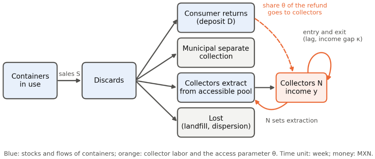
Figure 2.
Share of simulated systems in which a design is viable (recovery at least ρ*, collectors at least 90% of baseline), by deposit D and collector share θ. Left: κ from ENOE; right: κ ≥ 0. Top: ρ* = 0.7; bottom: ρ* = 0.8. Solid line: 0.5; dashed line: 0.9; orange circles: the two reported designs. 1,200 systems per panel.
Figure 2.
Share of simulated systems in which a design is viable (recovery at least ρ*, collectors at least 90% of baseline), by deposit D and collector share θ. Left: κ from ENOE; right: κ ≥ 0. Top: ρ* = 0.7; bottom: ρ* = 0.8. Solid line: 0.5; dashed line: 0.9; orange circles: the two reported designs. 1,200 systems per panel.
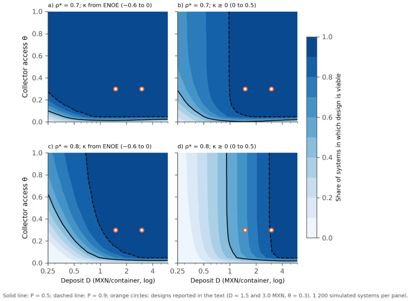
Figure 3.
Total-order Sobol indices at D = 1.5, θ = 0.3 for (a) recovery rate and (b) collectors relative to baseline, for the six largest inputs, under the two κ ranges.
Figure 3.
Total-order Sobol indices at D = 1.5, θ = 0.3 for (a) recovery rate and (b) collectors relative to baseline, for the six largest inputs, under the two κ ranges.
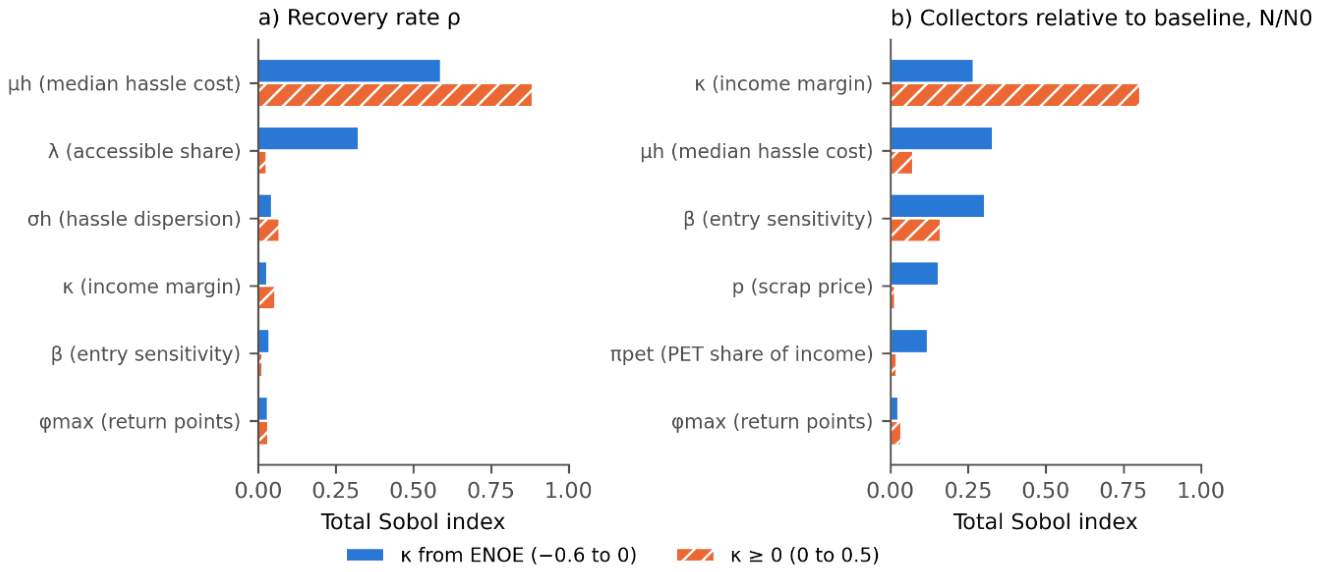
Table 2.
Uncertain inputs and ranges (uniform in the sampling). Status as in Table 1.
Table 2.
Uncertain inputs and ranges (uniform in the sampling). Status as in Table 1.
| Input | Meaning | Range | Status |
| μh | ln of the median hassle cost (MXN) | −0.7 to 1.8 | Scenario |
| σh | Dispersion of hassle cost | 0.3 to 1.5 | Scenario |
| φmax | Maximum direct-return share | 0.6 to 0.98 | Scenario |
| s | Collector share of baseline recovery | 0.4 to 0.8 | Scenario |
| λ | Share of non-returned containers accessible to collectors | 0.7 to 0.95 | Scenario |
| πpet | Share of collector income from PET | 0.1 to 0.5 | Scenario |
| κ | Income margin over the alternative | −0.6 to 0 (ENOE); 0 to 0.5 (initial) | ENOE calculation |
| β | Sensitivity of entry to the income gap | 2 to 8 | Scenario |
| mc | Bottle mass (kg) | 0.021 to 0.030 | Upper end anchored (Schwanse, 2011, p. 975) |
| ε | PET per collector (kg/day, six days/week) | 2 to 20 | Partly anchored: survey bands are for all materials; PET-only values and the 2 kg lower end are scenarios (Tagle Zamora and Rodríguez González, 2024, p. 18) |
| p | Scrap price (MXN/kg) | 1.5 to 4.5 | Anchored (Schwanse, 2011; Favela Ávila et al., 2013; Ramírez Báez, 2019) |
| c/p | Variable cost as share of price | 0 to 0.3 | Scenario |
| f/(y₀ + f) | Fixed cost as share of income before that cost (0.3 equals f/y₀ = 0.43) | 0 to 0.3 | Scenario |
| τL | Adjustment time of entry (weeks) | 13 to 52 | Scenario (no effect at steady state) |
| τp | Income perception time (weeks) | 4 to 16 | Scenario (no effect at steady state) |
Fixed: ρ₀ = 0.64, annual sales of PET 860,000 t, six working days per week, four weeks in use before discard.
Table 3.
Smallest deposit in the grid (MXN) at which at least 90% of simulated systems are viable, by collector share θ. “≤ 0.25” means the lowest grid value already satisfies it; “none” means no deposit in the grid reaches 90%.
Table 3.
Smallest deposit in the grid (MXN) at which at least 90% of simulated systems are viable, by collector share θ. “≤ 0.25” means the lowest grid value already satisfies it; “none” means no deposit in the grid reaches 90%.
| θ | ρ* = 0.7, ENOE κ | ρ* = 0.7, κ ≥ 0 | ρ* = 0.8, ENOE κ | ρ* = 0.8, κ ≥ 0 |
| 0 | none | none | none | none |
| 0.1 | 0.55 | 1.22 | 1.82 | 3.09 |
| 0.3 | ≤ 0.25 | 1.07 | 1.07 | 3.09 |
| 0.5 | ≤ 0.25 | 1.07 | 0.94 | 3.09 |
| 1.0 | ≤ 0.25 | 1.07 | 0.72 | 3.09 |
Table 4.
Reason for failure at the reference designs, ρ* = 0.8, θ = 0.3 (1,200 systems per range; percent of systems).
Table 4.
Reason for failure at the reference designs, ρ* = 0.8, θ = 0.3 (1,200 systems per range; percent of systems).
| Design | κ range | Viable | Recovery below target only | Collectors below 90% only |
| D = 1.5 | ENOE (−0.6 to 0) | 95.0 | 4.4 | 0.6 |
| D = 1.5 | κ ≥ 0 (0 to 0.5) | 67.8 | 31.8 | 0.4 |
| D = 3.0 | ENOE (−0.6 to 0) | 99.2 | 0.3 | 0.6 |
| D = 3.0 | κ ≥ 0 (0 to 0.5) | 91.4 | 8.2 | 0.4 |
Collector numbers in the simulations are not small: at (1.5, 0.3) the median ratio of collectors to baseline is 1.31 with κ ≥ 0 (5th to 95th percentile 1.05 to 1.84) and 2.55 with ENOE κ (1.52 to 5.21). The ENOE figure is not a forecast. It is a consequence of the entry rule: when κ is negative, the calibration needs a latent pool of potential entrants larger than the baseline number of collectors, Npool = N₀/Λ(βκ) > N₀, and a deposit that raises collector income draws on that pool. No data tell us how large that pool is. For this reason we regard the ENOE-κ results as the optimistic end of our range and the κ ≥ 0 results as the conservative end, and report both.
Table 5.
Pilot measurements, what they identify and the decision rule supported by the model.
| Measurement | Identifies | Rule (at D = 1.5, θ = 0.3; ρ* = 0.8) | Basis |
| Return share at three or more deposit levels | φmax, μh, σh | Below 0.4: consumer-response problem (viable in 44% to 92% of systems). 0.4–0.8: viable in all simulated systems. Above 0.8: raise θ and monitor collectors | Section 3.2 and Section 4.1 |
| Collector access and income; collector counts | Realized θ; κ; β; λ | θ ≥ 0.1 needed; compare income with the ENOE benchmark; track exits | Section 2.2 and Section 3.1 |
| Audited recovery | ρ | Compare with 0.7 and 0.8 on an agreed denominator | Section 2.1 |
Disclaimer/Publisher’s Note: The statements, opinions and data contained in all publications are solely those of the individual author(s) and contributor(s) and not of MDPI and/or the editor(s). MDPI and/or the editor(s) disclaim responsibility for any injury to people or property resulting from any ideas, methods, instructions or products referred to in the content. |
© 2026 by the authors. Licensee MDPI, Basel, Switzerland. This article is an open access article distributed under the terms and conditions of the Creative Commons Attribution (CC BY) license (http://creativecommons.org/licenses/by/4.0/).
Copyright: This open access article is published under a Creative Commons CC BY 4.0 license, which permit the free download, distribution, and reuse, provided that the author and preprint are cited in any reuse.