
Submitted:
30 October 2026
Posted:
02 November 2026
You are already at the latest version
Abstract
Haul road condition is recognised as a driver of tyre wear, fuel consumption and maintenance cost of mining haulage vehicles, but its link to reliability is usually stated qualitatively. Road surface irregularities are classified by wavelength and amplitude, and a dimensionless roughness index Q is defined from defect density and amplitude; for the categories of a published microprofile classification it gives Q ≈ 0.15, 0.50 and 1.00 for good, moderate and poor roads. Reliability is modelled by an additive hazard, which yields R(t|Q) = R0(t)exp(-γQt): the relative reliability decays exponentially in Q at a rate proportional to mission time and remains a probability for all Q ≥ 0. Parameters are estimated by Poisson regression of failure counts on exposure by road category, and a closed-form rule gives the number of failures needed to detect a given rate ratio (about 200 for a 1.5-fold difference at 80 % power). The case data comprise 2737 daily downtime records for four CAT 773E haul trucks at the Sayak mine from 1 January 2023 to 30 September 2026 and 251 component-monitoring records as of 1 September 2026. Consolidation of consecutive records with the same truck and classifier gives 295 technical episodes; tyre-related events are the largest group (30.2 %), while transmission and final-drive events account for 72.5 % of technical downtime. Because the records contain no exposure by road category, they characterise downtime structure and replacement priorities but do not quantify the road effect; a data collection protocol for doing so is proposed. Mid-range speeds of the road categories imply 33 % and 129 % longer travel times on moderate and poor roads.
Keywords:
haul roads
; mining haulage vehicles
; reliability
; road roughness
; additive hazard model
; Poisson regression
; spare parts
; underground mining
1. Introduction
Haulage vehicles - rigid-frame dump trucks in open pits, load-haul-dump (LHD) machines and underground trucks in underground mines - operate on unpaved roads built from local materials. Their availability and operating cost depend strongly on road condition: potholes, corrugations, rutting and loose material increase rolling resistance, impose shock and vibration loads on tyres, suspension, frame and on-board equipment, and force operators to reduce speed [1,2,3]. Field vibration measurements on large surface haulage trucks were used to derive test specifications for their on-board electronic equipment [4], and engine load, which grows with total motion resistance, is a principal factor of truck fuel consumption [5]. Mine road maintenance management systems therefore link road defect scores with vehicle operating costs and use the link to schedule grading [1].
These relationships are usually expressed as empirical cost functions or as qualitative recommendations. For reliability, the question has a definite mathematical form: how does the failure intensity of a vehicle or of its subsystem depend on a measurable characteristic of the road, and how can this dependence be estimated from maintenance records? An answer needs three elements: a metrologically defined roughness measure; a reliability model in which this measure enters as a covariate and which remains a valid probability model; and an estimation procedure that accounts for the exposure (operating hours or distance) accumulated on each road category. Standard tools exist for each element - profile-based roughness indices such as the International Roughness Index (IRI) and the spectral classification of road profiles [6,7], and covariate hazard models [8,9,10] - but they are rarely combined for mine haulage.
The aim of this study is to build such a combination and to apply it to the data available from a road microprofile classification [11] and from maintenance records of the Sayak mine (Kazakhstan). The contributions are: (i) a roughness index computed from defect density and amplitude; (ii) a reliability model derived from an additive hazard, its properties and its relation to the proportional hazards model; (iii) maximum-likelihood estimators and a sample-size rule for identifying the road effect from failure counts and exposure; (iv) an analysis of the technical downtime structure and component replacement priorities of the Sayak fleet. The scope covers surface and underground haul roads: the defect classes are common to both, whereas vehicle types and speeds differ, and the origin of each data set is stated explicitly.
2. Materials and Methods
2.1. Data. Three Data Sets Are Used
(a) Road-condition scenarios. Table 1 gives approximate ranges of defect density and dimensions for four categories of unpaved roads. The ranges are used as literature-informed engineering scenarios consistent with visual defect surveys and haul-truck response monitoring [1,2,3,11]; defect counts are normalised to a 1-km section and are not presented as measurements from Sayak. (b) Speeds. The ranges in Table 2 are approximate scenario values for surface haul trucks. Their use follows the performance-handbook principle that attainable speed depends on rolling resistance, grade, payload and local conditions [2,3,13]. (c) Sayak maintenance records. The AIC Monitoring extract contains 2737 daily downtime records for four CAT 773E trucks (fleet numbers 261, 300, 524 and 526) from 1 January 2023 to 30 September 2026 [16]. Consecutive calendar-day records with the same truck and classifier are treated as one episode. Planned maintenance, reserve status and external constraints are separated from technical episodes. The component-monitoring extract dated 1 September 2026 contains 251 component records for 50 equipment units assigned to Sayak or ShPT Sayak [15]. Neither data set contains operating exposure by road category.
2.2. Classification of Road Irregularities
The response of a vehicle to an irregularity depends on its wavelength Lw relative to the wheelbase and on speed. Four wavelength classes are distinguished: impulsive irregularities, Lw ≤ 0.3 m (stones, edges, short bumps), which act on tyres and unsprung masses as force impulses; potholes, 0.3 m < Lw ≤ 6 m, subdivided into short (0.3-1.0 m) and long (1.0-6.0 m) ones, which excite vertical accelerations of unsprung and sprung masses; undulations, 6 m < Lw ≤ 25 m, which cause low-frequency body motion whose intensity grows with speed; and macro-geometry, Lw > 25 m (grade and vertical curvature). Macro-geometry affects tractive effort and fuel consumption rather than vibration; it is a property of road alignment, not of roughness, and is excluded from the roughness index. By amplitude h, the classification distinguishes micro-texture, h ≤ 0.01 m, largely absorbed by large-diameter tyres; irregularities, 0.01 m < h ≤ 0.3 m; and obstacles, h > 0.3 m, which require a reduction to minimum speed to avoid suspension bottoming and wheel lift-off. Four road categories are defined by defect density and by the attainable average speed V relative to Vmax: good (lightly worn), V > 0.7Vmax; moderate (moderately worn), 0.4Vmax < V ≤ 0.7Vmax; poor (broken), 0.2Vmax < V ≤ 0.4Vmax; critical (rough terrain), V ≤ 0.2Vmax.
2.3. Roughness Index
For a road section, let nc be the number of defects of class c per kilometre and hc their most probable amplitude (height or depth). The defect intensity and the roughness index are defined as
where wc are class weights (wc = 1 in this paper) and Dref is the defect intensity of a reference category; here the poor category is the reference, so that Q = 1 on a poor road.
The quadratic dependence on amplitude makes Q a root-mean-square type measure, consistent with spectral roughness measures in which the variance of the profile elevation is the integral of its power spectral density. When profile measurements are available, the index should be computed from the profile itself:
where Gd(n) is the displacement power spectral density of the profile [7], n is the spatial frequency, and [n1, n2] = [0.04; 3.3] cycles/m corresponds to wavelengths from 25 to 0.3 m. Indices (2) and (3) should be cross-calibrated on the same sections; IRI [6] can serve as a widely reported third reference.
2.4. Reliability Model
Let T be the time to failure of a vehicle (or subsystem) operated on a road with index Q, t the operating time (engine hours; distance may be used instead), and λ(t|Q) the hazard rate. The additive hazard model [9] is
where λ0(t) is the hazard on an ideal road (Q = 0) and γ is the road sensitivity of the vehicle class, measured in units of λ per unit of Q. Integration of (4) gives
λ(t | Q) = λ0(t) + γQ, γ ≥ 0, Q ≥ 0,
For a fixed mission time t the relative reliability is
Equation (6) is the dependence plotted in Figure 2 of the first version of this paper; it replaces the expression R = R0 + exp(-kQ) given in the text of that version, which is not a probability model (Remark 1).
Proposition 1.Under (4), for all t ≥ 0 and Q ≥ 0 such that R0(t) > 0: (a) 0 < R(t|Q) ≤ R0(t) ≤ 1, with equality R(t|Q) = R0(t) at Q = 0; (b) R(t|Q) is non-increasing in t and in Q; (c) for Q2 > Q1 the ratio R(t|Q2)/R(t|Q1) = exp(-γ(Q2 - Q1)t) depends on the indices only through their difference and decreases exponentially with t.
Proof. Statements (a) and (b) follow from (5), because γQt ≥ 0 and R0 is a survival function; (c) follows by division of the two expressions (5). ∎
Remark 1. For R = R0 + exp(–kQ) with 0 < R0 < 1 and k > 0, R > 1 if and only if Q < –ln(1 - R0)/k. For R0 = 0.9 and k = 1 this holds for Q < 2.30, i.e. over the whole practical range of Q (Table 1).
The parameter k in (6) is therefore not a property of the suspension alone: it is the product of the road sensitivity γ and the mission time. The exponential decay of reliability under a linear growth of roughness is a consequence of the linear hazard assumption (4), not an empirical finding, and has to be tested on data (Section 2.5). When the baseline hazard is constant, λ0(t) ≡ λ0, the mean time to failure is
so the dimensionless ratio γ/λ0 is the relative increase of failure intensity per unit of Q. An alternative is the proportional hazards model [8], λ(t|Q) = λ0(t)exp(αQ), for which
R(t | Q) = R0(t)exp(αQ).
For small αQ, exp(αQ) – 1 ≈ αQ, and (8) reduces to (5)–(6) with k ≈ αΛ0(t), where Λ0(t) = –ln R0(t). The two models diverge at large Q and can be discriminated by information criteria once failure data by road category are available.
2.5. Parameter Estimation and Design of Observations
Let operating records be grouped by road category j = 1, …, J with index Qj, exposure Ej (operating hours accumulated on roads of category j) and number of failures Nj. Under (4) with constant λ0 the counts are independent Poisson variables,
with log-likelihood ℓ(λ0, γ) = Σj[Nj ln(λ0 + γQj) – Ej(λ0 + γQj)] + const, which is maximised subject to λ0 > 0, γ ≥ 0 [10]. For J = 2 and N2/E2 ≥ N1/E1 the maximum-likelihood estimators are explicit:
Nj∼Poisson(Ej (λ0 + γQj)), j = 1,…,J,
If N2/E2 < N1/E1, the constraint is active: γ̂ = 0 and λ̂0 = ΣNj/ΣEj. The same scheme with a logarithmic link gives the estimator of α in (8), and subsystem parameters are obtained by applying (9) to the failures of each subsystem. Exposure is indispensable: failure counts without Ej do not identify γ.
To plan observations, consider the rate ratio θ = λ(Q2)/λ(Q1) between two categories and the exposure ratio ρ = E2/E1. By the delta method, Var(ln θ̂) ≈ 1/N1 + 1/N2, and a two-sided test at significance level a with power 1 – b detects θ if
where zp is the p-quantile of the standard normal distribution.
2.6. Spare-Part Demand
Let the times between successive failures of a component that is replaced at failure be independent, with mean M, standard deviation σ and coefficient of variation ν = σ/M. The number of failures N(t) during operating time t is a renewal process; by the renewal central limit theorem [12], N(t) is asymptotically normal with mean t/M and variance ν2t/M. The stock that covers demand over a horizon t (lead time plus review period) with probability p is
where up is the normal quantile and ⌈·⌉ denotes rounding up. The normal law in (12) describes the number of failures over the horizon, not the time to failure; time to failure is described by the Weibull or lognormal laws [10].
2.7. Operational Indicators
Travel time per unit distance is 1/V. If φ is the share of travel time in the haul cycle on a good road and VG is the speed on that road, the productivity on a road with speed V(Q) relative to a good road is
On a haul segment of length L with grade i (positive uphill) and rolling resistance coefficient f, the tractive work for gross vehicle mass m is W = mg(f + i) L. A change of f from f1 to f2 therefore changes the tractive energy, and at constant drivetrain efficiency the fuel use, by the factor
3. Results
3.1. Roughness Index of the Road Categories
Table 1 gives the defect data with the row groups assigned to defect classes. The assignment follows from the parameter ranges: heights of 0.03–0.10 m at densities up to more than 200 per km correspond to impulsive irregularities, lengths of 0.5–5.0 m to potholes, and a small number of deep irregularities to long irregularities. This operational assignment is based on the stated dimensional ranges and is used only for the scenario calculation; it should be verified by measured longitudinal profiles in future field work. At mid-range values, (1)-(2) give D = 0.21, 2.30 and 9.19 m2/km and Q = 0.15, 0.50 and 1.00 for good, moderate and poor roads; for rough terrain, with open-ended values taken at their lower bounds, D = 25.1 m2/km and Q = 1.65 (D = 15.3 m2/km and Q = 1.29 if all its values are taken at the lower bounds). To assess the effect of the ranges, densities and amplitudes were sampled uniformly within them (400 000 draws, Dref fixed at 9.19 m2/km). The 90 % intervals of Q - 0.08-0.21, 0.35-0.68 and 0.84-1.18 - do not overlap, so the index separates the categories. The values assigned to the categories in the first version of the paper (0.2, 0.5 and 1.0) agree with (2) within the uncertainty of Table 1. On good, moderate and poor roads, potholes contribute 68-86 % of D; long irregularities become significant on poor roads (26 %) and dominate on rough terrain (about 70 %).
3.2. Operational Indicators
Table 2 combines the speed data with the quantities that follow from them. At mid-range speeds of 40, 30 and 17.5 km/h, travel time per kilometre is 1.50, 2.00 and 3.43 min, i.e. 33 % and 129 % longer on moderate and poor roads than on good ones. For a travel-time share φ = 0.5-0.7 (an illustrative range), Eq. (13) gives a productivity of 0.81-0.86 on moderate and 0.53-0.61 on poor roads relative to good roads. Reference rolling resistance coefficients for radial tyres are 2.5 % on a firm, smooth, maintained road flexing slightly under load, 4.0 % on a rutted dirt road with 25 mm tyre penetration and 5.0 % with 50 mm penetration [13]. By (14), an increase from 2.5 % to 4.0 % raises the tractive energy by 60 % on a level haul and by 14 % on an 8 % ramp; an increase to 5.0 % raises it by 100 % and 24 %, respectively. These reference values describe penetration and flexing of the road surface; their correspondence to Q has to be established by measurement (coast-down tests or on-board engine and payload data).
3.3. Technical Downtime Structure of the Sayak Fleet
The records contain 2737 daily downtime entries for four CAT 773E haul trucks. Consolidation of consecutive entries with the same truck and classifier gives 1395 episodes, of which 295 are technical (Figure 1). Tyres account for 89 technical episodes (30.2 %), followed by electrical equipment (45; 15.3 %), body and auxiliary equipment (43; 14.6 %), engine (41; 13.9 %), hydraulics (40; 13.6 %), transmission and final drives (18; 6.1 %), brakes (16; 5.4 %) and frame (3; 1.0 %). Technical downtime totals 8712.5 h. Transmission and final-drive events account for 6318.8 h (72.5 %), and tyre events for 855.6 h (9.8 %). A further 81 episodes classified as absence of spare parts account for 10739.0 h and are treated as supply-related delays rather than failures [16].
Road-induced vibration and shock can contribute to hydraulic and electrical failures through fatigue and abrasion of hoses and loosening of fittings – the reason why routing, clamping and abrasion protection are emphasised in hose assembly practice (SAE J1273) – through pressure peaks in cylinders under wheel impacts, and through chafing of wiring harnesses, wear of connector contacts and failures of sensors [4]. In the Sayak log, tyre damage is recorded explicitly under puncture or sidewall cut, tube, excessive wear and other tyre causes. Tyres form the largest group by technical episode count, while transmission and final-drive events dominate downtime hours. These patterns identify priority subsystems but do not prove that road roughness caused the events, because the records contain no road-section identifier, roughness measurement or exposure by road category. The ambiguous term “stabbing” is not used in the Sayak classifiers and has therefore been removed from the interpretation [16].
3.4. Time between failures and spare-part demand. For the illustrative spare-parts calculation retained in Table 3, the time between failures has mean M = 167.4 and standard deviation σ = 181.4. Their ratio gives ν = σ/M = 1.08; the value ν = 1.79 reported in the first version is inconsistent with M and σ (it would require σ = 300 at M = 167.4) and is not used. Three conclusions follow. First, a normal time-to-failure model is inadequate: with these moments it assigns probability Φ(–M/σ) = 0.18 to negative times. Second, ν slightly above unity is consistent with a Weibull law with shape parameter 0.92 and scale 161 (in the units of M) or with a lognormal law with logarithmic standard deviation 0.88. Third, ν > 1 is a signature of heterogeneity.
Proposition 2.Let T be exponentially distributed given a random failure rate Λ > 0 with a non-degenerate distribution and E[Λ–2] < ∞. Then ν(T) > 1.
Proof. Since E[T|Λ] = 1/Λ and E[T2|Λ] = 2/Λ2, ν2 = 2E[Λ–2]/(E[Λ–1])2 - 1, and E[Λ–2] > (E[Λ–1])2 by Jensen’s inequality for a non-degenerate Λ. ∎
Pooling machines or operating conditions with different failure intensities - including different road conditions – thus raises ν above unity, and a Weibull shape parameter below unity should not be read as infant mortality. This is compatible with a road effect but does not identify it, because machine type and duty cycle also vary across the fleet.
Table 3 gives the stock (12) for horizons τ = t/M = 6, 12 and 30. A simulation of a Weibull renewal process with the above moments (400 000 replications) gives the same stock as (12) in all six cases, which validates the normal approximation in this range. With the inconsistent value ν = 1.79, the stock would be overstated by 2-7 units (13-27 %).
3.5. Reliability as a Function of Road Condition
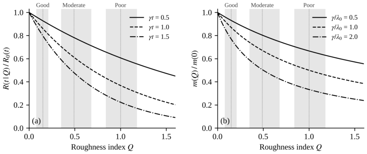
Figure 2 shows the relative reliability (6) and the relative mean time between failures (7) with the intervals of Q from Table 1. For γt = 1, the probability of failure-free operation over a mission on a poor road is exp(-(1.00 - 0.15)) = 0.43 of that on a good road (Proposition 1c); for γ/λ0 = 1, the mean time between failures on a poor road is (1 + 0.15)/(1 + 1.00) = 0.58 of that on a good road. These values illustrate the model; the parameters γ and λ0 of the Sayak fleet cannot be estimated from the available records (Section 3.6).
Figure 2.
Relative reliability (a) and relative mean time between failures (b) versus roughness index Q under the additive hazard model, Eqs. (6)-(7); shaded bands - 90 % intervals of Q for road categories (Table 1).
Figure 2.
Relative reliability (a) and relative mean time between failures (b) versus roughness index Q under the additive hazard model, Eqs. (6)-(7); shaded bands - 90 % intervals of Q for road categories (Table 1).
3.6. Data required to identify the road effect. Figure 3 shows rule (11) for a = 0.05 and power 0.8. A 1.5-fold difference in failure intensity between two road categories is detected with about 200 failures in total at ρ = 1 (80 of them on the better road), a 1.3-fold difference with about 460, and a 1.2-fold difference with about 950. The 295 reconstructed Sayak technical episodes are of a useful order of magnitude, but they cannot be used directly in (9) because operating exposure by road category was not recorded. The following protocol makes this possible: (i) divide the haul network into sections and measure Q on each by (2) or (3), repeating the measurement after grading; (ii) record operating hours and distance by vehicle and section from dispatch or GPS data; (iii) record each failure with time, vehicle, subsystem and failure mode; (iv) estimate (9) for each subsystem, compare models (4) and (8) by the Akaike information criterion, and include payload, speed and grade as additional covariates.
4. Discussion
The results separate what the available data establish from what they do not. The roughness index (2) turns the categorical description of roads into a number that orders the categories consistently and can be measured on any section; model (4)–(6) gives the road effect a definite form with a single interpretable parameter γ; rules (10)–(11) state what has to be recorded to estimate it. Road maintenance management systems for mines [1,3] already use defect scores to relate road condition to vehicle operating costs; the present formulation adds a probability-consistent reliability component that can be estimated from the same maintenance data, separately for each subsystem.
The main limitation is the linkage between the data sets. The values of Table 1 are literature-informed scenarios rather than measurements on Sayak roads. The downtime records identify trucks, dates and classifiers but not engine-hour exposure or road sections, while the component monitor describes current installed-component status rather than a completed replacement history. Consequently, the paper does not report an estimate of γ, and statements about the size of the road effect remain conditional on its value.
Once γ and the speed and fuel relations are estimated, the economic effect of road maintenance follows from the net present value of the avoided costs:
where the terms in the numerator are the annual savings in fuel, repairs, downtime and tyres obtained when the road index is reduced from Q1 to Q2 (computed from (7), (13), (14) and the measured tyre life), I is the cost of grading and compaction, r is the discount rate and H is the horizon; the payback period is the smallest H for which NPV ≥ 0.
5. Conclusions
1. A roughness index computed from the density and the squared amplitude of surface defects orders the road categories of the microprofile classification as 0.15, 0.50 and 1.00 (good, moderate, poor), with non-overlapping 90 % intervals, and can be cross-calibrated with profile-based measures.
2. An additive hazard model gives a reliability function R(t|Q) = R0(t)exp(–γQt) that is a valid probability for all Q ≥ 0; the exponential dependence of relative reliability on Q follows from the model assumptions, and its rate equals the road sensitivity multiplied by mission time.
3. The road sensitivity is estimated by Poisson regression of failure counts on exposure by road category; about 200 failures suffice to detect a 1.5-fold difference in failure intensity between two categories.
4. For four CAT 773E trucks at Sayak, tyres account for 30.2 % of 295 reconstructed technical episodes, while transmission and final-drive events account for 72.5 % of 8712.5 technical downtime hours. The component monitor identifies 100 overdue and 15 critical replacements among 251 component records.
5. The available records do not contain exposure by road category, so the road effect on reliability is not quantified here; the proposed protocol of section-level roughness measurement and exposure recording makes its estimation possible. Future work will apply it to haul trucks and LHDs on measured road sections.
Author Contributions
Ibrayeva Aisholpan: Conceptualization, methodology, formal analysis, investigation, data curation, visualization, writing-original draft preparation, and writing-review and editing: [please specify individual author contributions before submission]. All authors have read and agreed to the published version of the manuscript.
Funding
This research received no external funding.
Data Availability Statement
The operational datasets used in this study are internal company records and are not publicly available. Additional information may be available from the corresponding author upon reasonable request and with permission from the data owner.
Conflicts of Interest: The authors declare no conflicts of interest.
References
- Thompson, R.J.; Visser, A.T. Mine haul road maintenance management systems. J. South Afr. Inst. Min. Metall. 2003, 103(5), 303–312. [Google Scholar]
- Tannant, D.D.; Regensburg, B. Guidelines for mine haul road design; School of Mining and Petroleum Engineering, University of Alberta: Edmonton, 2001. [Google Scholar]
- Thompson, R.J.; Peroni, R.; Visser, A.T. Mining haul roads: theory and practice; CRC Press/Balkema: Leiden, 2019. [Google Scholar]
- Gagliardi, J.C.; Utt, W.K. 1993. Vibration environmental testing for large haulage trucks . Report of Investigations 9483. U.S. Department of the Interior, Bureau of Mines: Washington, DC. [Google Scholar]
- Kecojevic, V.; Komljenovic, D. Haul truck fuel consumption and CO2 emission under various engine load conditions. Min. Eng. 2010, 62(12), 44–48. [Google Scholar]
- Sayers, M.W.; Gillespie, T.D.; Paterson, W.D.O. Guidelines for conducting and calibrating road roughness measurements . In World Bank Technical Paper No. 46.; The World Bank: Washington, DC, 1986. [Google Scholar]
- ISO 8608:2016; Mechanical vibration - Road surface profiles - Reporting of measured data. International Organization for Standardization: Geneva.
- Cox, D.R. Regression models and life-tables. J. R. Stat. Soc. Ser. B (Methodological) 1972, 34(2), 187–220. [Google Scholar] [CrossRef]
- Aalen, O.O. A linear regression model for the analysis of life times. Stat. Med. 1989, 8(8), 907–925. [Google Scholar] [CrossRef] [PubMed]
- Meeker, W.Q.; Escobar, L.A. Statistical methods for reliability data; Wiley: New York, 1998. [Google Scholar]
- Thompson, R.J.; Visser, A.T.; Heyns, P.S.; Hugo, D. Mine road maintenance management using haul truck response measurements. Min. Technol. 2006, 115(4), 123–128. [Google Scholar] [CrossRef]
- Cox, D.R. Renewal theory; Methuen: London, 1962. [Google Scholar]
- Caterpillar, Inc. Rolling resistance factors . Available online: https://www.cat.com/en_US/articles/ci-articles/rolling-resistance-factors.html (accessed on 10 October 2026).
- Clopper, C.J.; Pearson, E.S. The use of confidence or fiducial limits illustrated in the case of the binomial. Biometrika 1934, 26(4), 404–413. [Google Scholar] [CrossRef]
- Kazakhmys Maintenance Services LLP. Component monitoring dataset as of 1 September 2026: Sayak and ShPT Sayak equipment. Intern. Oper. Dataset 2026. [Google Scholar]
- Kazakhmys Corporation LLP. AIC Monitoring downtime records for CAT 773E haul trucks at the Sayak mine, 1 January 2023-30 September 2026. Intern. Oper. Dataset 2026. [Google Scholar]
- Shakenov, A.; Sładkowski, A.; Stolpovskikh, I. Haul road condition impact on tire life of mining dump truck. Nauk. Visnyk Natsionalnoho Hirnychoho Universytetu 2022, 6, 25–29. [Google Scholar] [CrossRef]
- Richardson, S.; McIver, J. Improving Mine Haul Road Roughness to Reduce Haul Truck Fuel Consumption. SAE Tech. Pap. 2015, 2015-01-0050. [Google Scholar] [CrossRef]
Figure 1.
Distribution of technical downtime episodes by subsystem, four CAT 773E haul trucks at the Sayak mine, 1 January 2023-30 September 2026 (N = 295; error bars - 95 % Clopper-Pearson intervals).
Figure 1.
Distribution of technical downtime episodes by subsystem, four CAT 773E haul trucks at the Sayak mine, 1 January 2023-30 September 2026 (N = 295; error bars - 95 % Clopper-Pearson intervals).
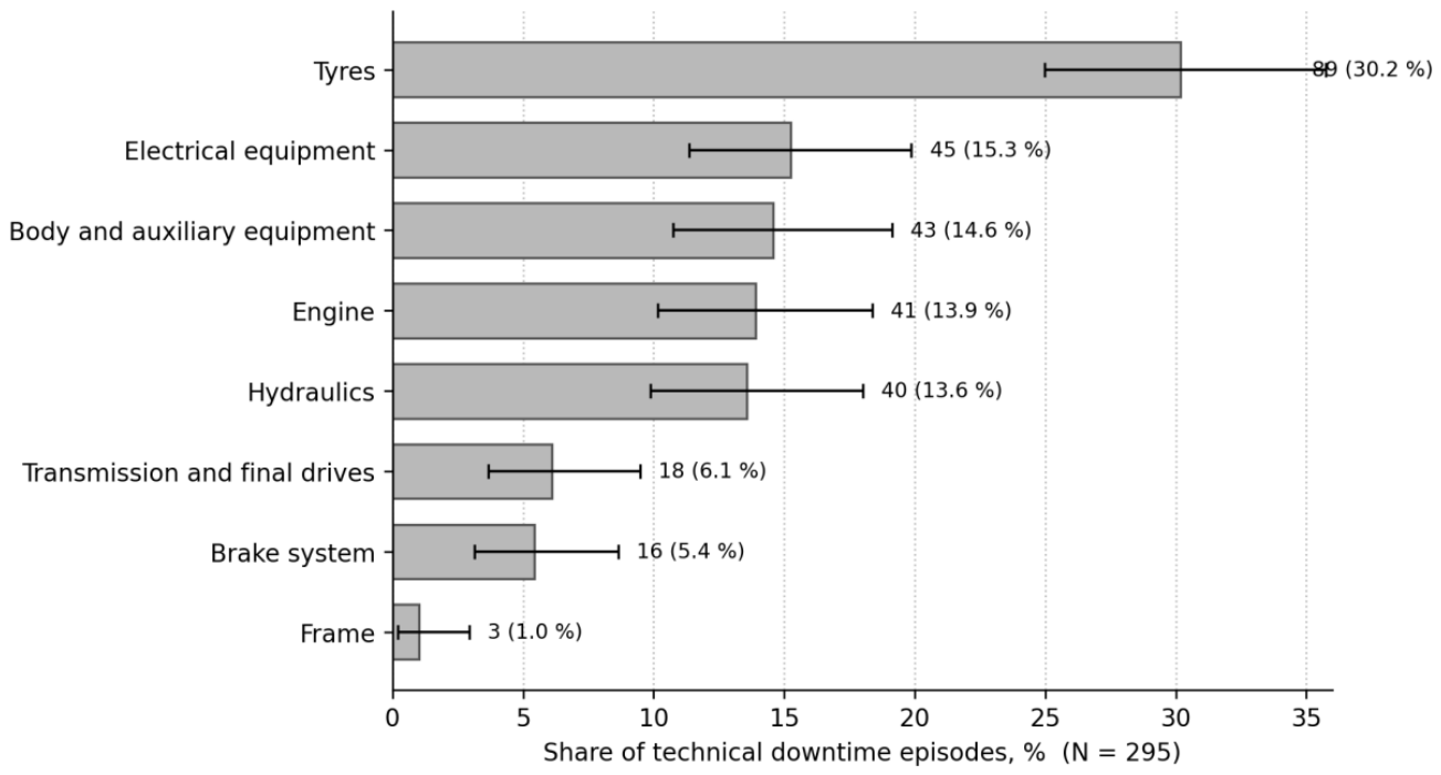
Figure 3.
Total number of failures required to detect a rate ratio θ between two road categories (two-sided test, significance level 0.05, power 0.8) for exposure ratios ρ = E2/E1; horizontal line – 295 reconstructed Sayak technical episodes, shown for scale.
Figure 3.
Total number of failures required to detect a rate ratio θ between two road categories (two-sided test, significance level 0.05, power 0.8) for exposure ratios ρ = E2/E1; horizontal line – 295 reconstructed Sayak technical episodes, shown for scale.
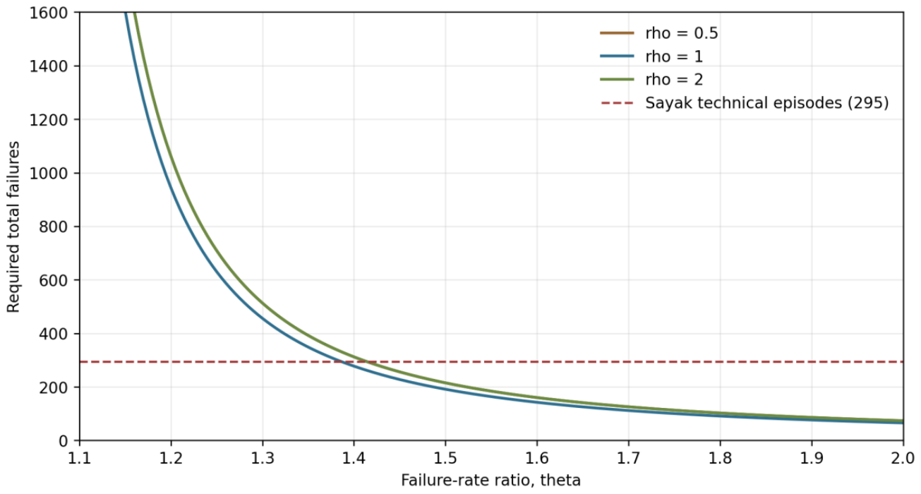

Table 1.
Surface defects per 1 km and roughness index by road category.
| Defect class and parameter | Good (lightly worn) | Moderate (moderately worn) | Poor (broken) | Critical (rough terrain) |
| Impulsive irregularities*, count per km | 20-50 | 50-150 | 100-200 | > 200 |
| - most probable height, m | 0.03-0.04 | 0.03-0.05 | 0.05-0.07 | 0.07-0.10 |
| Potholes*, count per km | ≤ 200 | 200-500 | 300-500 | 200-300 |
| - most probable length, m | 0.5-1.5 | 1.0-2.5 | 1.5-3.0 | 1.5-5.0 |
| - most probable depth, m | 0.03-0.05 | 0.05-0.10 | 0.10-0.15 | > 0.15 |
| Long irregularities*, count per km | ≤ 5 | 5-10 | 10-20 | > 20 |
| - most probable depth, m | 0.03-0.05 | 0.10-0.20 | 0.30-0.50 | 0.70–1.20 |
| Defect intensity D, m2/km, Eq. (1) | 0.21 | 2.30 | 9.19 | 25.1 |
| Roughness index Q, Eq. (2) | 0.15 | 0.50 | 1.00 | 1.65 |
| 90 % interval of Q | 0.08-0.21 | 0.35-0.68 | 0.84-1.18 | - |
* Assignment of row groups to defect classes is inferred from the stated dimensional ranges. The values are literature-informed scenario inputs [1,2,3,11], not verified measurements from the Sayak mine; D and Q are computed at mid-range values, with “≤” ranges read from zero and open-ended rough-terrain values taken at their lower bounds.
Table 2.
Operational indicators of haul trucks by road category.
| Indicator | Good | Moderate | Poor | Critical | Refs. |
| Speed class, V/Vmax | > 0.7 | 0.4-0.7 | 0.2-0.4 | ≤ 0.2 | 2 |
| Average speed, km/h | 35-45 | 25-35 | 10-25 | 5-10 | 2 |
| Travel time at mid-range speed, min/km | 1.50 | 2.00 | 3.43 | 8.00 | 2 |
| Increase in travel time vs good road, % | 0 | 33 | 129 | 433 | 2 |
| Relative productivity at φ = 0.5–0.7 | 1 | 0.81-0.86 | 0.53-0.61 | 0.25-0.32 | 2 |
| Roughness index Q | 0.15 | 0.50 | 1.00 | 1.65 | 11 |
| Failure intensity, failures per 1000 h | 0.8-1.0 | 1.1-1.4 | 1.5-2.0 | 2.1-3.0 | 11 |
| Tyre life, h | 5.5-7.0k | 4.0-5.5k | 2.5–4.0k | 1.5-2.5k | 17 |
| Fuel consumption, L/h | 50-65 | 60-80 | 75–100 | 90-125 | 18 |
Table 3.
Spare-part stock np by Eq. (12) for a component with M = 167.4, σ = 181.4.
| Horizon τ = t/M | Service level p | Eq. (12), ν = 1.08 | Eq. (12), ν = 1.79 | Simulation, Weibull, ν = 1.08 |
| 6 | 0.90 | 10 | 12 | 10 |
| 6 | 0.95 | 11 | 14 | 11 |
| 12 | 0.90 | 17 | 20 | 17 |
| 12 | 0.95 | 19 | 23 | 19 |
| 30 | 0.90 | 38 | 43 | 38 |
| 30 | 0.95 | 40 | 47 | 40 |
Disclaimer/Publisher’s Note: The statements, opinions and data contained in all publications are solely those of the individual author(s) and contributor(s) and not of MDPI and/or the editor(s). MDPI and/or the editor(s) disclaim responsibility for any injury to people or property resulting from any ideas, methods, instructions or products referred to in the content. |
© 2026 by the authors. Licensee MDPI, Basel, Switzerland. This article is an open access article distributed under the terms and conditions of the Creative Commons Attribution (CC BY) license (http://creativecommons.org/licenses/by/4.0/).
Copyright: This open access article is published under a Creative Commons CC BY 4.0 license, which permit the free download, distribution, and reuse, provided that the author and preprint are cited in any reuse.