

Submitted:
30 October 2026
Posted:
02 November 2026
You are already at the latest version
Abstract
This study examines household lighting expenditure, lighting-energy efficiency and the adoption of energy-efficient appliances in Uganda. Using the 2025 survey data on 410 households, we estimate a stochastic cost frontier for monthly expenditure on all lighting sources and linear probability, logit and probit models of appliance adoption. Our results show that lighting expenditure rises with the number of rooms, hours of electricity availability, mobile payment use and energy-efficiency awareness. However, it is associated with the household head’s age, rural residence, renting, and monthly income above UGX 1,000,000 (US$300). Moreover, the mean efficiency score is 0.59, so the minimum expenditure predicted for comparable households averages 59% of observed expenditure, while regional means range from 0.55 in Eastern to 0.72 in Toro. Furthermore, awareness and training raise the predicted probability of adoption by 39.6 and 23.3 percentage points, respectively, whereas rural residence lowers it by 18.0 percentage points. Income, secondary education, age, household size and mobile money ownership also raise adoption. Energy policy in Uganda should therefore pair reliable electricity supply with practical energy efficiency trainings, quality-assured efficient products and payment arrangements that spread upfront costs.
Keywords:
household lighting
; lighting expenditure
; expenditure efficiency
; stochastic frontier analysis
; appliance adoption
; Uganda
1. Introduction
Lighting is a basic household energy service that supports children’s study, domestic work, home-based enterprise and personal safety after dark (Hirmer & Guthrie, 2017). Nonetheless, how households obtain light differ widely in cost and quality. Fuel-based lighting costs its users about US$ 38 billion a year, or roughly US$ 77 per household, yet it delivers only about 0.1% of the world’s lighting services (Mills, 2005). Moreover, the household lighting market is changing rapidly, as rural African households have moved from kerosene to inexpensive LED lamps powered by disposable dry-cell batteries, largely without government or donor support (Bensch et al., 2017). In this setting, households’ ability to obtain adequate lighting at the lowest attainable cost has become an important determinant of household welfare. This ability can be termed lighting-expenditure efficiency, which refers to a household’s observed spending on all energy sources used for lighting relative to the minimum expenditure predicted for households with comparable observed characteristics. Also, efficiency in this sense differs from low energy use or low energy intensity, which are poor indicators of how efficiently households obtain energy services (Filippini & Hunt, 2015). When households move closer to this minimum, they can obtain the same illumination with fewer purchases of electricity tokens, kerosene, candles, and batteries, freeing up income for food, schooling, and other needs.
Nonetheless, it remains unclear what drives household lighting expenditure and how far households spend above the minimum required for their circumstances. Boogen (2017) finds that Swiss households are, on average, about 20% to 25% inefficient in their electricity use. Moreover, the mean efficiency score in Ghana was 63.0% for the entire sample and 69.9% and 66.3% for rural and urban households, respectively (Twerefou & Abeney, 2020). In sub-Saharan Africa (SSA), the evidence on lighting expenditure itself is mixed. Grimm et al. (2017) find that low-cost solar kits in rural Rwanda increased lighting consumption, measured in lumen-hours, and reduced spending on kerosene and small batteries. However, Lenz et al. (2017) show that appliance uptake and electricity use stayed low after a large expansion of grid connections in Rwanda. Furthermore, Meles (2020) finds that power outages in urban Ethiopia push households to spend on candles, kerosene, batteries and generators, with coping costs that can reach about 60% of the average electricity bill. Part of this disagreement reflects measurement, as electricity-wide studies combine lighting with cooking, refrigeration, entertainment, and other services, and exclude the non-electric sources that many households use for lighting. A further explanation is provided by the fuel-stacking perspective, in which households combine several energy sources rather than abandoning traditional sources as their incomes rise (Masera et al., 2000). As a result, studies of electricity use or of a household’s main lighting source may misrepresent total lighting expenditure and conceal large differences between households.
According to the World Bank (2026), 55.1% of the population in SSA had access to electricity in 2024, compared with 91.9% globally. Moreover, access varied considerably within the region, reaching only 35.7% in rural areas compared with 82.9% in urban areas, as shown in Figure 1. Kojima et al. (2016) also report that only about one-third of people in twenty-two SSA countries use electricity and that affordability, rather than proximity to the grid, is often the main barrier to use. Moreover, wealthier and better-educated households in Ethiopia, Malawi and Tanzania are more likely to use electricity or solar lighting, whereas poorer households rely on kerosene and batteries (Rahut et al., 2017). The region’s lighting challenge should therefore be considered alongside the constraints facing its households. Specifically, limited purchasing power restricts the adoption of efficient technologies even when lifetime savings are large. For instance, low-income households in Nairobi were willing to pay only about US$12 for an efficient cookstove that would save about US$237 over its two-year life, while access to credit more than doubled their willingness to pay (Berkouwer & Dean, 2022). Furthermore, a Pay As You Go Solar Home System offers the potential to deliver a disruptive positive impact with regard to increasing access to clean, affordable energy for the poor in the Central region of East Africa because such a system spreads costs over small weekly instalments paid by scratch card or mobile money (Barrie & Cruickshank, 2017).
In Uganda, the Energy Transition Plan, launched in 2023, commits the country to universal access to electricity and cleaner cooking by 2030. Also, the Electricity Connections Policy for 2018 to 2027 covers the cost of connection materials for households ready to use electricity and aims to raise grid access to 60% by 2027. Moreover, the National Energy Policy for Uganda 2023 provides the wider framework for these targets, while the Fourth National Development Plan (NDP IV) and the Tenfold Growth Strategy treat energy as a key driver of Uganda’s goal of a US$500 billion economy by 2040. Nonetheless, only 55.3% of the population had access to electricity in 2024, with 78.3% in urban areas but only 44.8% in rural areas (Figure 1). In rural homes, access is held back by high upfront connection costs and unreliable supply. Energy poverty is correspondingly widespread. About 66% of Ugandans are multidimensionally energy poor, 33% are severely so, and the energy poor are deprived on 51% of the weighted indicators on average (Ssennono et al., 2021).
Existing Ugandan studies have examined the household energy mix (Lee, 2013), the drivers of solar photovoltaic adoption (Aarakit et al., 2021; Aarakit et al., 2022), the drivers of energy efficiency among grid-connected households in Kampala (Watundu et al., 2022) and household electricity efficiency using stochastic frontier analysis (Mubiinzi et al., 2026). Nonetheless, little is known about how much Ugandan households spend on lighting across all sources, or how close that spending is to the minimum attainable for comparable households. Moreover, it remains unclear which household and dwelling characteristics are associated with lighting expenditure, and how far that expenditure exceeds this minimum across regions. Also, evidence on the adoption of energy-efficient appliances beyond solar photovoltaic systems, such as efficient lighting products and improved cookstoves, remains limited.
Against this background, the present study examines household lighting expenditure, lighting-expenditure efficiency and the adoption of energy-efficient appliances in Uganda. First, we examine the household and dwelling factors associated with monthly lighting expenditure. Second, we estimate and compare lighting-expenditure efficiency scores across regions. Third, we investigate the factors associated with energy-efficient appliance adoption, using an indicator that also covers appliances beyond lighting, such as improved cookstoves. Moreover, our study makes three contributions. First, it provides lighting-specific evidence from a 2025 household survey by measuring expenditure on all lighting sources rather than on electricity or the main source alone. Second, it offers conditional expenditure benchmarks that separate spending attributable to household circumstances from excess spending, so that low spending is not mistaken for efficient lighting. Third, it adds evidence on energy-efficient appliance adoption that can guide awareness, training and financing programmes. Finally, Section 2 reviews the theoretical and empirical literature, Section 3 presents the methodology and data, Section 4 reports the results, Section 5 discusses them, and Section 6 concludes with policy recommendations.
2. Literature Review
2.1. Theoretical Framework
This study combines consumer demand and household production theory, the economic approach to measuring energy efficiency, the energy-ladder and fuel-stacking perspectives, and theories of technology adoption. Consumer demand theory holds that households allocate limited budgets among goods and services to maximise utility subject to prices, available technologies and other constraints (Deaton & Muellbauer, 1980). Moreover, household production theory treats purchased goods as inputs that households combine with their own time to produce the commodities from which they derive utility (Becker, 1965). Similarly, Lancaster (1966) argues that consumers value the characteristics that goods provide rather than the goods themselves. In our framework, households obtain utility from illumination rather than from electricity, solar power, kerosene, batteries or candles, so the demand for these energy sources is derived from the demand for the lighting service. Lighting expenditure therefore reflects the quantity of lighting a household requires, the technologies it uses to convert energy into light and the prices it pays for each source. However, demand theory alone does not explain why households with similar characteristics spend different amounts to obtain comparable lighting.
The economic approach to energy efficiency addresses this heterogeneity. Filippini and Hunt (2011) model energy demand as a stochastic frontier, in which the frontier represents the minimum energy required to provide a given level of energy services and deviations above it reflect inefficiency. Filippini and Hunt (2015) further argue that efficiency should be measured relative to such a production-theory-based frontier, rather than by energy intensity or low consumption. Accordingly, we define lighting-expenditure efficiency as the ratio of the minimum expenditure predicted for a household with given characteristics to the household’s observed expenditure. A cost-efficient household minimises spending on the energy sources used for lighting for a given lighting service and installed technology, whereas an inefficient household spends more than this conditional minimum, for example through costly backup sources, inefficient bulbs or unfavourable purchasing arrangements. Furthermore, the stochastic frontier separates this household-specific excess expenditure from random shocks such as measurement error, price fluctuations and supply interruptions (Aigner et al., 1977). Nevertheless, low expenditure does not, by itself, indicate efficiency, as a household may spend little when its access is constrained, or its demand for lighting is suppressed.
The energy-ladder hypothesis predicts that households move from traditional fuels towards modern energy as their incomes rise and infrastructure improves (Leach, 1992). However, the fuel-stacking perspective holds that households often retain several sources simultaneously to manage costs, reliability, and task-specific needs rather than switching completely from one source to another (Masera et al., 2000). In the lighting context, households may combine grid electricity with solar lanterns, torches, candles or kerosene lamps, especially where electricity supply is unreliable. The frontier in our study is therefore defined over expenditure on all lighting sources rather than on the principal source alone. Also, the energy ladder implies that income, location and electricity availability shape both the choice of lighting sources and the level of lighting expenditure.
Technology adoption theory explains why households adopt energy-efficient appliances unevenly. Diffusion theory emphasises relative advantage, compatibility, complexity, trialability and observability as determinants of adoption, with information and communication channels shaping how quickly new technologies spread (Rogers, 1975). Moreover, the energy-efficiency gap literature shows that households often fail to adopt efficient technologies that appear cost-effective, owing to information problems, principal–agent problems and other market and behavioural barriers (Jaffe & Stavins, 1994). Allcott and Greenstone (2012) also identify imperfect information, inattention and credit constraints as possible sources of underinvestment in energy efficiency, although they find that the evidence on the size of the gap is mixed. In our framework, an energy-efficient appliance lowers the energy input required per unit of service and can move a household towards the expenditure frontier. A household adopts when the expected lifetime savings exceed the purchase cost, and it has the information, liquidity, and market access needed to act. Hence, awareness, training, income, education, mobile money, and location are included in our adoption models.
Based on the framework above, we test the following hypotheses, each corresponding to one objective. H1 posits that lighting expenditure rises with the scale of a household’s lighting needs, captured by the number of rooms, and with hours of electricity availability. H2 states that observed lighting expenditure exceeds the conditional minimum, so that household-specific excess expenditure is present in the composite error and mean efficiency differs across regions. H3 states that energy-efficiency awareness, training, income and access to mobile money raise the probability that households adopt energy-efficient appliances.
2.2. Empirical Literature
It has been established that households rarely use energy at the minimum level required for the services they obtain. For instance, Filippini and Hunt (2012) estimate a stochastic demand frontier for residential energy across 48 United States states and show that energy intensity is a poor proxy for underlying energy efficiency. Boogen (2017) finds that Swiss households are, on average, about 20% to 25% inefficient in their electricity use. Moreover, Andor et al. (2021) report a mean efficiency of about 0.83 for residential electricity consumption in Germany. Furthermore, Boogen et al. (2021) find that energy-related financial literacy is associated with lower inefficiency among households in Italy, the Netherlands and Switzerland. However, Broadstock et al. (2016) find that efficiency does not increase with wealth among Chinese households, with the wealthiest city households being the least efficient. In developing economies, Twerefou and Abeney (2020) report a mean electricity-use efficiency of 63.0% for Ghanaian households. Moreover, Nsangou et al. (2020) report a mean efficiency of 62.4% for households in Cameroon, while Basumatary et al. (2024) report a mean efficiency of 77.25% for rural households in India. In Uganda, Watundu et al. (2022) estimate a mean technical efficiency of 0.66 among grid-connected households in Kampala. These studies measure the efficiency of electricity use or total residential energy use, and none of them measures expenditure across all the sources households use for lighting.
The evidence on dwelling size and the characteristics of the household head is mixed. Blasch et al. (2017) find that dwelling size raises electricity demand among Swiss households. Moreover, Sakah et al. (2019) find that larger floor area is associated with higher electricity consumption among urban Ghanaian households. However, Basumatary et al. (2024) find that the number of living rooms does not increase household electricity consumption in rural India. The evidence on age is also inconclusive. Estiri and Zagheni (2019) find that residential energy consumption in the United States increases over the life course, largely through larger housing. Twerefou and Abeney (2020) find that an older household head is associated with lower electricity-use efficiency in Ghana. Conversely, Otsuka (2017) finds no significant association between ageing and residential electricity efficiency across Japanese prefectures. Similarly, the evidence on gender is unsettled. Rahut et al. (2017) find that female-headed households in Ethiopia, Malawi and Tanzania are more likely to use clean lighting sources. However, Adusah-Poku et al. (2023) find that female-headed households in Ghana are more likely to choose cleaner energy if they have the characteristics of male-headed households, suggesting that the gender gap reflects differences in endowments rather than headship itself. Nevertheless, Frederiks et al. (2015) conclude from a review that the effects of gender on residential energy consumption are inconsistent, minimal or statistically insignificant.
Location and housing tenure also shape household energy expenditure. Lee (2013) finds that income, education and public infrastructure shape the Ugandan household energy mix, with differing effects in rural and urban areas. Moreover, Kojima et al. (2016) find that electricity users in SSA are disproportionately urban and better off, and that affordability limits use where the grid is available. Furthermore, Nsangou et al. (2020) find that rural households in Cameroon use electricity more efficiently than urban households, whereas Otsuka (2017) finds that the most densely populated Japanese prefectures are the most efficient. Turning to tenure, Andor et al. (2021) find that owners in Germany tend to use electricity more efficiently than tenants, although the difference is not robustly significant. Yohanis et al. (2008) also find that electricity use is higher in owner-occupied than in rented dwellings in Northern Ireland. However, Klege et al. (2022) find that rental status has varying effects on cooking and lighting fuel choices in Rwanda, with inconclusive results for lighting.
The availability and reliability of electricity affect lighting expenditure. Lenz et al. (2017) find that grid connection in Rwanda reduced the use of dry-cell batteries and lowered household energy expenditure, while electricity use and appliance uptake remained low. Moreover, Meles (2020) finds that outages push urban Ethiopian households into costly coping spending on candles, kerosene, batteries and generators. Furthermore, Sedai et al. (2021) find that each additional hour of daily electricity supply raises household consumption, income and assets in India, so the reliability of supply matters beyond connection. Twerefou and Abeney (2020) also find that power outages are associated with lower electricity-use efficiency in Ghana. Similarly, Watundu et al. (2022) find that holding a backup energy source is associated with higher inefficiency among grid-connected households in Kampala. Basumatary et al. (2024) also find that longer and more frequent power cuts increase inefficiency in rural household electricity use in India.
Income and financial access shape lighting choices and expenditure. Lay et al. (2013) find a cross-sectional energy ladder in lighting fuel choice in Kenya, although kerosene use falls only among the richest households and access to the grid and to solar home systems also shapes the choice. Moreover, Addai et al. (2022) find that access to financial services raises the consumption of lighting energy, including electricity, batteries and lanterns, in rural Ghana. Furthermore, Aarakit et al. (2022) find that financial inclusion, with mobile money as its most important component, raises the adoption of solar photovoltaic systems in Uganda. Munyegera and Matsumoto (2016) also find that mobile money adoption is positively associated with household consumption in rural Uganda. Barrie and Cruickshank (2017) show that pay-as-you-go financing allows low-income households to acquire solar home systems through small instalments. Similarly, Berkouwer and Dean (2022) find that credit more than doubles low-income Nairobi households’ willingness to pay for an efficient cookstove. Nonetheless, Broadstock et al. (2016) caution that higher income does not automatically translate into more efficient energy use.
The evidence on energy-efficiency awareness and information is generally positive but not uniform. Blasch et al. (2017) find that energy literacy and, more strongly, investment literacy are associated with lower electricity consumption among Swiss households. Moreover, Boogen et al. (2021) associate energy-related financial literacy, mainly through its cognitive component, with lower inefficiency. In Uganda, Watundu et al. (2022) find that households that understand energy-efficiency labels are less inefficient, although this association is significant only at the 10% level. Furthermore, Delmas et al. (2013) find that audits and consulting yield the largest savings among information strategies, at about 13.5%, compared with an average of 7.4% across 156 trials. However, Filippini et al. (2014) find that informative measures are not significantly associated with underlying residential efficiency across European Union countries, whereas financial incentives are.
Evidence on the adoption of energy-efficient appliances points to the need for information, resources, and market access. Marin and Palma (2017) find that the technology embedded in major household appliances, much of it transferred internationally, is associated with more efficient residential electricity use across European countries. Moreover, Blasch et al. (2019) find that households with higher energy and investment literacy are more likely to identify the appliance with the lowest lifetime cost. Blasch et al. (2022) also find that a short education module and an online lifetime-cost calculator both improve this choice. Furthermore, Mills and Schleich (2012) find that education increases the adoption of energy-efficient technologies across European countries, whereas households with many elderly members adopt them less. Mills and Schleich (2014) also show that German households increased luminosity by 23% after switching to compact fluorescent lamps and by 47% after switching to LEDs. However, Schleich (2019) finds that low-income households are less likely than high-income households to adopt LEDs and efficient appliances across eight European countries. In developing economies, Amoah et al. (2018) find that environmental consciousness, education and income are associated with the choice of energy-saving bulbs in Ghana. Zou and Mishra (2020) find that income, household size and dwelling area raise the purchase of labelled energy-efficient appliances in rural China. In SSA, Kamuzora (2024) finds that lighting choices in rural Tanzania vary with the age, sex, marital status, and employment of the household head, as well as with household size. Wassie et al. (2021) also find that cleaner lighting in rural southern Ethiopia is associated with higher income, more education and road access, while income and grid connection do not end the use of traditional fuels. In Uganda, Aarakit et al. (2021) find that affordability, flexible payment options, education, rural residence, and grid access shape household adoption of solar photovoltaic systems.
Three gaps follow from this review. First, the frontier studies reviewed measure the efficiency of electricity use or total residential energy use, and none measure expenditure across the full set of sources households use for lighting, which fuel stacking makes necessary in settings such as Uganda. Second, the direction of the associations for age, gender, location and tenure differs across settings, and Ugandan evidence on the determinants of lighting expenditure, as distinct from electricity consumption or source choice, is scarce. Third, Ugandan adoption studies concentrate on solar photovoltaic systems, whereas evidence on the broader set of energy-efficient appliances, including efficient lighting products and improved cookstoves, remains limited. The present study addresses these gaps by estimating a stochastic cost frontier for expenditure on all lighting sources in Uganda, deriving household and regional efficiency scores, and examining the factors associated with the adoption of energy-efficient appliances.
3. Methodology and Data
We use cross-sectional survey data collected from 410 households in Uganda’s Central, Eastern, Northern, Ankole and Toro regions during 2025. The sampling frame comprised household lists obtained from village or cell council chairpersons in selected locations. Districts were selected purposively using UBOS poverty statistics, and the planned sample was allocated according to district population shares from the 2024 census. Within selected districts, the sampling procedure provided for equal rural and urban allocation, except in Kampala, which was treated as entirely urban. Households were then randomly selected from local lists using computer-generated numbers in Microsoft Excel. Trained research assistants administered structured questionnaires to household heads or spouses and recorded responses electronically using Kobo.
The questionnaire captured monthly expenditure on all lighting sources and household, dwelling, electricity access, financial and awareness characteristics. Ethical approval was obtained from Makerere University, the district headquarters, and the National Council for Higher Education. Respondents also provided written informed consent, with confidentiality and the right to withdraw protected. Our unit of analysis was the household. Monthly lighting expenditure was available for 407 households, of which 378 reported positive expenditure and complete information on the frontier variables. These households form the frontier sample. The remaining 29 observations were excluded because expenditure was zero or a frontier covariate was missing, while three households had no expenditure record. The adoption models use all 410 households because the adoption indicator and its covariates were complete. We report descriptive statistics using all available observations for each variable.
3.1. Stochastic Cost Frontier Model
Our empirical specification is grounded in the derived demand for lighting services. Following Filippini and Hunt (2011), the general form of the household lighting-expenditure function can be represented as:
where refers to monthly household expenditure on all energy sources used for lighting, measured in Uganda shillings, is a vector of observed household and dwelling characteristics, is a vector of unknown parameters, and is a composite error term. Equation 1 describes the expenditure a household incurs to obtain its lighting services, given its characteristics. To reduce the influence of extreme values and to interpret the coefficients as elasticities or semi-elasticities, we transform Equation 1 into natural logarithms to obtain a cross-sectional stochastic cost frontier at the household level:
Here, is a symmetric random error that captures measurement error, random price variation, supply shocks and other factors outside the household’s control, whereas is a one-sided error that captures household-specific excess expenditure. The positive sign on reflects a cost frontier, in which inefficiency raises expenditure above the conditional minimum, rather than the production frontier of Aigner et al. (1977), in which inefficiency lowers output. Accordingly, is the stochastic minimum, or frontier, expenditure for household . The specification we estimate is:
where is the number of rooms, is the age of the household head, equals 1 for rural households, equals 1 for female heads, equals 1 for rented dwellings, is the number of hours electricity was available during the preceding seven days, are indicators for the three upper monthly income categories, with income below UGX 100,000 as the reference group, equals 1 for households that make mobile payments, and equals 1 for households aware of energy-efficient appliances or practices. The number of rooms captures the scale of lighting needs, as larger dwellings require more lighting points (Sakah et al., 2019). Age captures life-cycle differences in energy use (Estiri & Zagheni, 2019), while gender captures differences in energy preferences between male- and female-headed households (Rahut et al., 2017). Moreover, location captures rural–urban differences in access and prices (Lee, 2013), and tenure captures differences in incentives between tenants and owners (Andor et al., 2021). Electricity availability captures the reliability of supply (Meles, 2020). Furthermore, income and mobile payments capture purchasing power and access to payment services (Addai et al., 2022), while awareness captures energy-related knowledge (Blasch et al., 2017). Expenditure, rooms and age enter in natural logarithms, so and are elasticities. For hours of electricity availability, approximates the percentage change in lighting expenditure associated with one additional hour. For binary variables and income categories, the exact percentage difference from the reference group is . The error components satisfy:
The half-normal distribution for follows Aigner et al. (1977). We define and . A value of close to zero indicates that deviations from the frontier arise mainly from random noise, whereas a larger value indicates that household-specific excess expenditure contributes substantially to the composite error. We also report , the share of the composite variance parameter attributable to the one-sided term. The parameters are estimated by maximum likelihood (Kumbhakar & Lovell, 2003), and for the half-normal cost frontier the log-likelihood function is:
where is the number of households, is the standard normal cumulative distribution function and . Household-specific excess expenditure is not observed directly. Following Jondrow et al. (1982), we recover it from the conditional distribution of given the composite residual:
where is the standard normal density function. Lighting-expenditure efficiency is the ratio of minimum conditional expenditure, , to observed expenditure:
A score of 1 place a household on the expenditure frontier. A score of 0.70, for example, indicates that the minimum expenditure predicted for a houehold with the same observed characteristics is 70% of the household’s actual expenditure. With denoting the estimated score, the efficient frontier lighting expenditure and the avoidable lighting-cost waste are:
Equations 8 and 9 express the efficiency score in monetary terms. The frontier expenditure in Equation 8 is the predicted minimum, given the household’s characteristics, and the waste in Equation 9 is the amount by which observed expenditure exceeds this minimum. Since both are computed household by household, their sample means sum to mean observed expenditure. We then compare mean scores across regions to assess whether excess expenditure differs across the country, which completes the test of H2.
3.2. Energy-Efficient Appliance Adoption Models
To examine the factors associated with the adoption of energy-efficient appliances, we model adoption as a binary outcome, with equal to 1 if the household uses energy-efficient appliances and 0 otherwise. The survey indicator covers appliances beyond lighting, including LED bulbs and improved cookstoves, so our adoption models describe broad energy-efficient appliance adoption rather than lighting technology alone. The probability of adoption is:
where Zi contains energy-efficiency awareness, energy-efficiency training, income, education of the household head, age, gender, household size, location, mobile money account ownership and the number of rooms, with income below UGX 100,000 and no education as the reference categories, and is a vector of parameters. Awareness and training capture information about efficient technologies (Blasch et al., 2019). Moreover, income and mobile money capture the ability to finance upfront costs (Aarakit et al., 2022), and education captures the capacity to process technical information (Mills & Schleich, 2012). Household size and location capture differences in energy needs and market access (Zou & Mishra, 2020). We estimate Equation 10 using three functional forms for . In the linear probability model, is the identity function:
where is the error term, so each coefficient measures the change in the probability of adoption directly. Also, in the logit and probit models, F(⋅) is the logistic and the standard normal cumulative distribution function, respectively:
The logit and probit models keep predicted probabilities between 0 and 1, whereas the linear probability model does not guarantee this. However, their coefficients do not measure changes in probability directly, so we report average marginal effects:
where is the density function corresponding to . For binary regressors, the marginal effect is the average discrete change in the predicted probability when the variable changes from 0 to 1, holding the other variables at their observed values. We express all marginal effects in percentage points. The logit and probit models are estimated by maximum likelihood, and comparing them with the linear probability model shows whether our conclusions depend on the functional form.
3.3. Estimation and Diagnostic Tests
Heteroskedasticity-robust standard errors are reported for all models (White, 1980). For the frontier, a Wald test examines the joint significance of the regressors, while the significance of σu and λ indicates whether the one-sided error term is present, which is the test of H2. We also report an ordinary least squares benchmark of Equation 3 without the one-sided error to show how the frontier changes the estimates. Pairwise correlations and variance inflation factors were examined for potential multicollinearity, without treating any single rule-of-thumb threshold as decisive (O’brien, 2007). For the linear probability model, the Breusch–Pagan test was used to assess heteroskedasticity (Breusch & Pagan, 1979), and the Ramsey RESET test was used to assess functional-form misspecification (Ramsey, 1969). All reported tests are two-sided. Table 1 describes the variables.
4. Results
4.1. Descriptive Statistics
Table 2 presents the descriptive statistics. Average monthly lighting expenditure among the 407 reporting households was UGX 14,719.32 (about US$3.98), with a standard deviation of UGX 15,755.31. Households had an average of 2.72 rooms and 4.53 members, while household heads averaged 38.76 years of age. Moreover, 63% of households were urban, 36% were female-headed, and 56% rented their dwellings. Electricity availability averaged 21.67 hours over the preceding seven days, with a standard deviation of 22.75 hours. Monthly income was UGX 100,000–500,000 for 50% of households, UGX 500,001–1,000,000 for 26%, above UGX 1,000,000 for 16% and below UGX 100,000 for 8%. Furthermore, 95% of households made mobile payments, and 97% had a mobile money account. Energy-efficiency awareness stood at 77%, while 11% of household heads had received energy-efficiency training. Half of the households used energy-efficient appliances, including LED bulbs. Also, 41% of household heads had secondary education, 35% had post-secondary education, 13% had primary education, and 10% had no education.
We present the principal lighting sources in Figure 2, which shows that electricity was the principal source for 85.37% of households, solar energy for 12.93%, and 1.71% reported no electricity. Although most households relied mainly on electricity, the limited weekly hours of availability reported in Table 2 indicate that many of them are likely to need other sources when supply is interrupted, consistent with the fuel-stacking perspective.
We report pairwise correlations among the study variables in Table A1 in the Appendix. Our results show that the correlations are generally modest. The highest correlation, 0.630, is between mobile payments and mobile money account ownership, but these two variables never appear in the same model, as mobile payments enter the frontier model and mobile money enters the adoption model. Moreover, housing tenure is negatively correlated with the number of rooms at −0.561 and with the age of the household head at −0.475, while household size is positively correlated with the number of rooms at 0.493. Low pairwise correlations do not by themselves rule out harmful multicollinearity, so we also examined variance inflation factors. The mean variance inflation factor of 1.25 is well below the conventional warning level of 10 (O’brien, 2007). Therefore, multicollinearity is unlikely to distort our estimates. Lighting expenditure is most strongly correlated with the number of rooms, at 0.189, followed by housing tenure, at −0.134, and electricity availability, at 0.130.
4.2. Stochastic Frontier Results
We present the stochastic frontier estimates for the 378 frontier households in Table 3, beside the ordinary least squares benchmark. The estimated standard deviations of the excess expenditure and noise components are 0.607 and 0.604, respectively, and both are significant at the 1% level. Moreover, is 1.004 and significant at the 1% level, and is 0.502, so excess expenditure and random variation contribute almost equally to the composite variance parameter. Taking the variance of the half-normal term, , household-specific excess expenditure accounts for about 26.8% of the variance of the composite error. These results support H2, as observed lighting expenditure contains a significant one-sided component above the conditional minimum. Furthermore, the Wald statistic of 82.60 is significant at the 1% level, so the explanatory variables are jointly associated with lighting expenditure. The ordinary least squares benchmark explains 12.7% of the variation in logged lighting expenditure, which shows that much of the variation is not explained by observed characteristics alone. The ordinary least squares and frontier coefficients agree in sign for every variable, while the frontier estimates are significant for age, rural location, tenure, and awareness, which are not significant in the benchmark. We focus our interpretation on the frontier estimates, and percentage differences for binary variables are computed as .
We first describe the dwelling and household characteristics. Our results show that the number of rooms has a frontier elasticity of 0.423, significant at the 1% level, so a 1% increase in the number of rooms is associated with a 0.42% increase in lighting expenditure, holding other factors constant. For instance, a household with three rooms spends about 18.7% more than a comparable household with two rooms. Conversely, the age of the household head has an elasticity of −0.336, significant at the 5% level, indicating that a 1% increase in age is associated with a 0.34% decrease in lighting expenditure. Thus, a household headed by a 50-year-old spends about 15.8% less than a comparable household headed by a 30-year-old. Moreover, rural households spend approximately 16.6% less on lighting than urban households, and households in rented dwellings spend approximately 22.4% less than owner-occupiers. Both associations are significant at the 5% level. The gender of the household head is not significant in either specification.
Furthermore, each additional hour of electricity availability in the preceding week is associated with approximately a 0.7% increase in lighting expenditure, significant at the 5% level. A one-standard-deviation increase of 22.75 hours is therefore associated with about 17.3% higher lighting expenditure. Among the income categories, only monthly income above UGX 1,000,000 is significant. These households spend approximately 47.5% less on lighting than households earning less than UGX 100,000, at the 1% significance level. The middle-income categories are negative but not significant. In contrast, households that make mobile payments spend approximately 63.7% more on lighting than households that do not, significant at the 1% level. Households that are aware of energy-efficient appliances or practices also spend approximately 20.9% more, although this association is significant only at the 10% level. Our results therefore support H1, as lighting expenditure rises significantly with the number of rooms and with hours of electricity availability. The ordinary least squares benchmark yields similar conclusions for rooms, electricity availability, the highest income category and mobile payments, with mobile payments associated with approximately 54.3% higher expenditure and the highest income category with approximately 46.8% lower expenditure.
We summarise the efficiency scores and the derived expenditure measures for the 378 frontier households in Table 4. Panel A shows that mean observed lighting expenditure in the frontier sample is UGX 15,848.58, or about US$4.28 per month, which exceeds the mean for all 407 reporting households, as households that reported zero expenditure are excluded. The mean efficiency score of 0.59 indicates that the minimum expenditure predicted for comparable households is, on average, 59% of observed expenditure. The mean predicted minimum expenditure is UGX 11,101.00, or about US$3.00, and the mean lighting-cost waste is UGX 4,747.58, or about US$1.28 per month. Over a year, this waste amounts to about UGX 56,971, or US$15.40, per household. The two means sum to the mean observed expenditure. Their ratio is 0.70 rather than 0.59, because the efficiency score is the average of household-level ratios in Equation 7, not the ratio of the two averages, and households with low expenditure and low scores weigh more heavily in the average of ratios.
Panel B shows that Toro records the highest mean score of 0.72, followed by Central at 0.60, while Ankole and Northern each record 0.58 and Eastern has the lowest score of 0.55. The 0.17 range between the highest and lowest regional means indicates that excess lighting expenditure is not uniform across the country, further supporting H2. Moreover, we present average monthly lighting expenditure and mean efficiency scores by study location in Figure 3. The fitted line slopes downwards, indicating that locations with higher average lighting expenditure tend to record lower average efficiency scores. For instance, Fort Portal City records the highest mean score of about 0.81, with average monthly lighting expenditure below UGX 5,000, whereas Mbale City records the lowest score of about 0.38, with average monthly lighting expenditure exceeding UGX 60,000. Nonetheless, several locations with similar average expenditure, such as Lira and Kabarole, record very different scores, so expenditure levels alone do not determine efficiency.
Energy-Efficient Appliance Adoption Results
We present the linear probability model estimates and the average marginal effects from the logit and probit models for all 410 households in Table 5, and we report the full logit and probit coefficients in Table A2 in the Appendix. The three models agree in sign for every variable, and every variable that is significant in one model is significant at least at the 10% level in the others. The linear probability model explains 31.2% of the variation in adoption. Its Breusch–Pagan statistic of 0.030 is not significant, so there is no evidence of heteroskedasticity, although we report robust standard errors throughout. However, its Ramsey RESET statistic of 2.100 is significant at the 10% level, indicating possible functional-form misspecification and supporting our reliance on the logit and probit marginal effects. The logit and probit marginal effects differ by at most 1.0 percentage point, so our conclusions do not depend on the choice between them. We therefore focus our interpretation on the logit marginal effects, expressed in percentage points.
We first describe the information variables. Our results show that energy-efficiency awareness raises the predicted probability of adoption by 39.6 percentage points, and training raises it by 23.3 percentage points, both significant at the 1% level. In odds terms, aware households have about 9.8 times the odds of adoption as unaware households, and trained households have about 4.1 times the odds of adoption as untrained households, as shown by the logit coefficients in Table A2. Moreover, relative to households earning less than UGX 100,000 per month, households earning UGX 100,000 to 500,000 and UGX 500,001 to 1,000,000 are 30.4 and 38.7 percentage points more likely to adopt, respectively, at the 1% significance level. Households earning above UGX 1,000,000 are 18.0 percentage points more likely to adopt, significant at the 5% level. The income gradient is therefore not monotonic, as the association is largest in the UGX 500,001-1,000,000 category and smaller in the highest category. Our results support H3, as awareness, training and income are positively and significantly associated with adoption.
Furthermore, secondary education of the household head raises the probability of adoption by 16.1 percentage points relative to no education, significant at the 5% level, whereas primary and post-secondary education are not significant. Each additional year of the household head’s age raises the probability by 0.5 percentage points, so a household head who is 10 years older is about 5 percentage points more likely to adopt. Each additional household member also raises the probability by 1.9 percentage points, and both associations are significant at the 5% level. Conversely, rural households are 18.0 percentage points less likely to adopt than urban households, significant at the 1% level. Owning a mobile money account increases the probability of adoption by 22.0 percentage points, which is significant at the 5% level, although the underlying logit and probit coefficients are significant only at the 10% level. This finding provides further support for H3. The gender of the household head and the number of rooms are not significant in any specification. Finally, the linear probability estimates are close to the marginal effects, with awareness, training and rural residence associated with 39.9, 21.7 and −18.6 percentage-point changes in the probability of adoption, respectively.
4.3. Discussion of the Findings
Our main finding is that lighting expenditure among Ugandan households is shaped first by the scale of lighting needs and by the availability of electricity, which supports H1. The positive elasticity of the number of rooms is consistent with Blasch et al. (2017), who find that dwelling size increases electricity demand among Swiss households. It also agrees with Sakah et al. (2019), who find that larger floor area is associated with higher electricity consumption in urban Ghana. However, it differs from Basumatary et al. (2024), who find that the number of living rooms does not increase rural electricity consumption in India. More rooms mean more lighting points and longer combined hours of use, so higher conditional expenditure in larger dwellings reflects greater lighting needs rather than waste. Similarly, the positive association between hours of electricity availability and lighting expenditure is consistent with Sedai et al. (2021), who show that additional hours of supply raise household consumption in India. Households with more reliable supply can use electric lighting for longer, so their expenditure rises with the quantity of lighting services they obtain. This interpretation is also consistent with Meles (2020), who finds that outages push households to spend on candles, kerosene, and batteries, suggesting that reliability changes both the composition and the level of lighting expenditure. Nonetheless, Lenz et al. (2017) find that grid connection lowered energy expenditure in Rwanda as electricity replaced dry-cell batteries. Our result concerns hours of supply among mostly connected households rather than connection itself, so the two findings are compatible.
Moreover, the significant one-sided error term supports H2. Our mean efficiency score of 0.59 is below the mean of about 0.83 reported by Andor et al. (2021) for German households and below the 63.0% reported by Twerefou and Abeney (2020) for Ghana. It is also below the 62.4% reported by Nsangou et al. (2020) for Cameroon and the 0.66 reported by Watundu et al. (2022) for grid-connected households in Kampala. We regard this comparison as indicative only, as our frontier covers expenditure on all lighting sources rather than metered electricity. Masera et al. (2000) show that households stack several sources, and the cost of backup lighting sources is one plausible reason why expenditure gaps for a complete lighting portfolio can exceed those for electricity alone. Furthermore, the regional range from 0.55 in Eastern to 0.72 in Toro is consistent with Ssennono et al. (2021), who find that energy poverty in Uganda varies strongly by region. Nonetheless, our data cannot attribute the regional gaps to prices, product availability or housing conditions.
Furthermore, the negative association between the age of the household head and lighting expenditure differs from Estiri and Zagheni (2019), who find that residential energy consumption in the United States increases over the life course. Nonetheless, our adoption models show that age is positively associated with the use of energy-efficient appliances, so lower expenditure among older heads may partly reflect their greater use of efficient technologies. The lower expenditure of rural households is consistent with Kojima et al. (2016), who find that electricity users in SSA are disproportionately urban and that affordability limits use. Filippini and Hunt (2015) caution that low consumption can reflect constrained access rather than efficiency, and rural households in our data are also less likely to adopt efficient appliances. Hence, lower rural expenditure is more plausibly attributable to limited access and suppressed demand than to efficient lighting. Similarly, the lower expenditure of tenants aligns with Yohanis et al. (2008), who find higher electricity use in owner-occupied than in rented dwellings in Northern Ireland. Our expenditure result does not by itself establish a difference in efficiency, and Watundu et al. (2022) find no significant association between renting and inefficiency in Kampala. Tenants may live in smaller dwellings with fewer fixtures, or their electricity costs may be shared with landlords or other tenants.
The lower expenditure of households earning above UGX 1,000,000 (US$300) differs from the cross-sectional energy ladder in lighting fuel choice reported by Lay et al. (2013) for Kenya. A plausible explanation is that the highest-income households own efficient bulbs, solar systems or appliances with lower running costs. Our adoption results are consistent with this reading, as every income category above the lowest is more likely to use energy-efficient appliances, although the survey does not record each household’s bulb stock. Moreover, this result is consistent with Schleich (2019), who finds that low-income households are less likely than high-income households to adopt LEDs. In contrast, higher lighting expenditure among households that make mobile payments is consistent with Addai et al. (2022), who find that access to financial services raises lighting energy consumption in rural Ghana. Munyegera and Matsumoto (2016) also find that mobile money adoption is positively associated with household consumption in rural Uganda, so mobile payments appear to ease the purchase of prepaid electricity and pay-as-you-go lighting services rather than to reduce spending.
The positive association between awareness and lighting expenditure contrasts with Blasch et al. (2017), who find that energy and investment literacy are associated with lower electricity consumption in Switzerland. One explanation is that aware households demand more and better illumination. This interpretation agrees with Mills and Schleich (2014), who find that German households increased luminosity by 23% to 47% after switching to efficient lamps. As awareness is also the strongest correlate of adoption, it appears to raise the quantity of lighting services purchased rather than lower their cost. Furthermore, the insignificance of the household head’s gender is consistent with Frederiks et al. (2015), who conclude that the effects of gender on residential energy consumption are inconsistent, minimal or statistically insignificant.
Finally, the adoption results support H3 and align with the literature on information, resources and market access. The large marginal effect of awareness agrees with Blasch et al. (2019), who find that energy and investment literacy help households identify the appliance with the lowest lifetime cost. Moreover, the effect of training agrees with Delmas et al. (2013), who find that audits and consulting produce the largest savings among information strategies. The positive associations of income and household size are consistent with Zou and Mishra (2020), who find that income and household size raise the purchase of labelled efficient appliances in rural China. Similarly, the positive association with secondary education agrees with Mills and Schleich (2012), who find that education raises the adoption of energy-efficient technologies in Europe, while the rural disadvantage agrees with Murungi et al. (2025), who identify high connection costs and unreliable supply as barriers to modern energy in rural Uganda. Furthermore, the positive association with mobile money agrees with Aarakit et al. (2022), who find that mobile money is the component of financial inclusion that matters most for solar adoption in Uganda. Berkouwer and Dean (2022) also show that credit constraints, rather than inattention, limit the adoption of efficient cookstoves among low-income households in Nairobi, pointing to the same liquidity mechanism.
5. Conclusions, Limitations, and Policy Recommendations
This study examined household lighting expenditure, lighting expenditure efficiency, and the adoption of energy-efficient appliances in Uganda. Using 2025 survey data on 410 households, we find that lighting expenditure rises with the number of rooms, hours of electricity availability, mobile payment use and energy-efficiency awareness, and falls with the age of the household head, rural residence, renting and monthly income above UGX 1,000,000. Moreover, the mean efficiency score of 0.59 indicates that the minimum expenditure predicted for comparable households averages 59% of observed expenditure, with a mean avoidable cost of about UGX 4,748 per household per month. Regional means range from 0.55 in Eastern to 0.72 in Toro. Furthermore, half of the surveyed households reported using energy-efficient appliances, and adoption was strongly associated with awareness, training, income, secondary education, age, household size, urban residence and mobile money account ownership. Our results support the prediction of the economic approach to energy efficiency that observed expenditure can exceed the conditional minimum, and the prediction of technology adoption theory that information and liquidity shape the use of efficient technologies.
Our study has limitations. First, our results are associations rather than causal effects, as the analysis relies on cross-sectional data and self-reported measures. Second, the survey does not record lighting prices, the stock and quality of bulbs or the quantity of light obtained, so some differences in lighting services may be attributed to excess expenditure. Third, the adoption indicator combines lighting appliances with other efficient appliances, such as improved cookstoves, so our adoption results cannot be attributed to lighting technologies alone. Fourth, the frontier excludes households with zero reported lighting expenditure, and the sample covers five regions, so the findings may not represent all Ugandan households. Future research could use panel data and direct measures of lighting services to address these limitations.
Consequently, our findings suggest that household energy programmes in Uganda should address the cost of lighting as well as access to electricity. First, the positive association between electricity availability and lighting expenditure, together with the lower expenditure of rural households, indicates that expanding reliable supply should be accompanied by measures that help households obtain useful lighting at lower lifetime cost. Consumer information should explain purchase price, expected energy savings, product life, quality and safe disposal in terms that households can apply when choosing bulbs and other appliances. Second, the large marginal effects of awareness and training on adoption, and the finding that awareness alone is associated with higher rather than lower lighting expenditure, justify practical demonstrations and community-based training linked to credible retailers and product-quality assurance, so that households can act on what they learn. Distribution and after-sales support for efficient bulbs, solar lighting products and compatible appliances should also extend beyond the major urban markets, given the lower adoption among rural households. Third, the positive associations of mobile payment use with lighting expenditure and of mobile money account ownership with adoption support payment arrangements that spread upfront costs, including instalment purchase, pay-as-you-go mechanisms and appropriately regulated consumer credit. Furthermore, the regional differences in efficiency scores justify locally adapted programmes and monitoring. Together, these findings suggest that reliable electricity, practical efficiency training, quality-assured products and flexible payment arrangements should be pursued together to lower the cost of household lighting in Uganda.
Author Contributions
Peter Babyenda conceptualised the study, analysed and drafted the manuscript. Diphus Tugume participated in data collection, cleaned the data and conducted statistical analyses and revised the manuscript. Lean Nancy Ankunda supervised data collection conducted literature review and reviewed the manuscript. Edward Bbaale supervised the analysis and revised the manuscript. All authors read and approved the final manuscript.
Funding
The study was funded by the Carnegie Corporation of New York through the Consolidating Early Career Academics Programme through Post-Doctoral Training (CECAP II, 2024 to 2027) at the Directorate of Research and Graduate Training, Makerere University.
Ethics Approval and Consent to Participate
The study received REC approval from Makerere University College of Business and Management Sciences REC (CoBAMS-REC).
Consent for Publication
All authors approved the manuscript for publication.
Availability of Data and Materials
The data used in this study are available from the corresponding author upon reasonable request for research and replication purposes only.
Competing Interests
The authors declare no competing interests.
Declaration of Generative AI and AI Assisted Technologies in the Writing Process
The authors used Copilot in the process of revising and improving the clarity, coherence, and overall readability of this manuscript. The authors carefully reviewed, edited, and approved all text generated through this process and take full responsibility for the content presented.
Acknowledgments
We thank the enumerators and research assistants for conducting household visits and supporting the survey.
Appendix

Table A1.
Pairwise correlations.
| Variables | (1) | (2) | (3) | (4) | (5) | (6) | (7) | (8) | (9) | (10) | (11) | (12) | (13) | (14) | (15) |
| (1) Lighting expenditure | 1.000 | ||||||||||||||
| (2) Rooms | 0.189 | 1.000 | |||||||||||||
| (3) Head age | 0.042 | 0.450 | 1.000 | ||||||||||||
| (4) Location | −0.031 | 0.102 | 0.037 | 1.000 | |||||||||||
| (5) Head gender | −0.009 | −0.096 | −0.068 | 0.005 | 1.000 | ||||||||||
| (6) Housing tenure | −0.134 | −0.561 | −0.475 | −0.238 | 0.097 | 1.000 | |||||||||
| (7) Electricity hours | 0.130 | −0.166 | −0.148 | 0.060 | −0.075 | 0.127 | 1.000 | ||||||||
| (8) Household income | −0.086 | −0.002 | −0.159 | −0.090 | −0.082 | 0.116 | 0.034 | 1.000 | |||||||
| (9) Mobile payments | 0.102 | 0.059 | −0.092 | −0.085 | 0.019 | 0.028 | −0.041 | 0.178 | 1.000 | ||||||
| (10) EE awareness | 0.093 | 0.139 | 0.067 | −0.052 | −0.108 | −0.024 | −0.059 | −0.019 | 0.155 | 1.000 | |||||
| (11) EE appliance use | 0.117 | 0.158 | 0.156 | −0.177 | −0.020 | −0.054 | −0.039 | −0.017 | 0.173 | 0.379 | 1.000 | ||||
| (12) EE training | 0.058 | 0.211 | 0.075 | −0.072 | 0.036 | −0.112 | −0.096 | −0.075 | 0.052 | 0.158 | 0.237 | 1.000 | |||
| (13) Head education | 0.052 | 0.074 | −0.113 | −0.199 | −0.045 | 0.070 | −0.023 | 0.307 | 0.149 | 0.192 | 0.085 | 0.031 | 1.000 | ||
| (14) Household size | 0.079 | 0.493 | 0.422 | 0.109 | −0.079 | −0.481 | −0.164 | −0.146 | −0.051 | −0.020 | 0.118 | 0.200 | −0.143 | 1.000 | |
| (15) Mobile money | 0.064 | −0.018 | −0.064 | −0.059 | −0.066 | 0.096 | 0.010 | 0.133 | 0.630 | 0.126 | 0.106 | 0.012 | 0.096 | −0.064 | 1.000 |
| Mean VIF | 1.25 |
Note. The table reports pairwise correlation coefficients for the study variables. Source. Authors’ computation based on the 2025 household survey data.
Table A2.
Logit and probit coefficients for energy-efficient appliance adoption.
| Variable | Logit | Probit |
| Energy-efficiency awareness (Yes) | 2.281*** (0.369) | 1.345*** (0.201) |
| Energy-efficiency training (Yes) | 1.416*** (0.464) | 0.821*** (0.255) |
| Household income (reference: less than 100,000) | ||
| 100,000 to 500,000 | 1.886*** (0.517) | 1.156*** (0.300) |
| 500,001 to 1,000,000 | 2.373*** (0.557) | 1.448*** (0.325) |
| Above 1,000,000 | 1.175** (0.595) | 0.718** (0.347) |
| Household head education (reference: no education) | ||
| Primary | −0.410 (0.483) | −0.262 (0.286) |
| Secondary | 0.928** (0.427) | 0.565** (0.252) |
| Post-secondary | −0.198 (0.454) | −0.083 (0.269) |
| Household head age | 0.028** (0.012) | 0.016** (0.007) |
| Household head gender (Female) | 0.313 (0.255) | 0.197 (0.150) |
| Household size | 0.114** (0.054) | 0.069** (0.032) |
| Location (Rural) | −1.045*** (0.259) | −0.625*** (0.153) |
| Mobile money (Yes) | 1.348* (0.697) | 0.818* (0.424) |
| Number of rooms | 0.039 (0.084) | 0.019 (0.049) |
| Constant | −6.708*** (1.115) | −4.030*** (0.646) |
| Observations | 410 | 410 |
Note. Robust standard errors in parentheses. *** p<0.01, ** p<0.05, * p<0.1. The dependent variable equals 1 if the household uses energy-efficient appliances and 0 otherwise. Average marginal effects are reported inTable 5. Source. Authors’ computation based on the 2025 household survey data.
| 1 | We calculate the dollar equivalent at UGX 3,700 per US$1, which gives approximate thresholds of less than US$27, US$27 to US$135, US$135 to US$270 and above US$270 per month. |
References
- Aarakit, S. M., J. M. Ntayi, F. Wasswa, M. S. Adaramola, and V. F. Ssennono. 2021. Adoption of solar photovoltaic systems in households: Evidence from Uganda. Journal of Cleaner Production 329: 129619. [Google Scholar] [CrossRef]
- Aarakit, S. M., J. M. Ntayi, F. Wasswa, F. Buyinza, M. S. Adaramola, and V. F. Ssennono. 2022. The role of financial inclusion in adoption of solar photovoltaic systems: A case of Uganda. Renewable Energy 198: 984–998. [Google Scholar] [CrossRef]
- Addai, B., W. Tang, M. A. Twumasi, D. Asante, and A. S. Agyeman. 2022. Access to financial services and lighting energy consumption: Empirical evidence from rural Ghana. Energy 253: 124109. [Google Scholar] [CrossRef]
- Adusah-Poku, F., S. Adams, and K. Adjei-Mantey. 2023. Does the gender of the household head affect household energy choice in Ghana? An empirical analysis. Environment, Development and Sustainability 25, 7: 6049–6070. [Google Scholar] [CrossRef]
- Aigner, D., C. A. K. Lovell, and P. Schmidt. 1977. Formulation and estimation of stochastic frontier production function models. Journal of Econometrics 6, 1: 21–37. [Google Scholar] [CrossRef]
- Allcott, H., and M. Greenstone. 2012. Is there an energy efficiency gap? Journal of Economic Perspectives 26, 1: 3–28. [Google Scholar] [CrossRef]
- Amoah, A., G. Hughes, and P. Pomeyie. 2018. Environmental consciousness and choice of bulb for lighting in a developing country. Energy, Sustainability and Society 8, 1: 17. [Google Scholar] [CrossRef]
- Andor, M. A., D. H. Bernstein, and S. Sommer. 2021. Determining the efficiency of residential electricity consumption. Empirical Economics 60, 6: 2897–2923. [Google Scholar] [CrossRef]
- Barrie, J., and H. J. Cruickshank. 2017. Shedding light on the last mile: A study on the diffusion of pay as you go solar home systems in Central East Africa. Energy Policy 107: 425–436. [Google Scholar] [CrossRef]
- Basumatary, S., M. Devi, K. Basumatary, and I. R. Basumatary. 2024. Household inefficient electricity consumption and its determinants in rural areas. Journal of Development Policy and Practice 11, 2: 238–252. [Google Scholar] [CrossRef]
- Becker, G. S. 1965. A theory of the allocation of time. The Economic Journal 75, 299: 493–517. [Google Scholar] [CrossRef]
- Bensch, G., J. Peters, and M. Sievert. 2017. The lighting transition in rural Africa—From kerosene to battery-powered LED and the emerging disposal problem. Energy for Sustainable Development 39: 13–20. [Google Scholar] [CrossRef]
- Berkouwer, S. B., and J. T. Dean. 2022. Credit, attention, and externalities in the adoption of energy efficient technologies by low-income households. American Economic Review 112, 10: 3291–3330. [Google Scholar] [CrossRef]
- Blasch, J., N. Boogen, M. Filippini, and N. Kumar. 2017. Explaining electricity demand and the role of energy and investment literacy on end-use efficiency of Swiss households. Energy Economics 68, S1: 89–102. [Google Scholar] [CrossRef]
- Blasch, J. E., M. Filippini, N. Kumar, and A. L. Martinez-Cruz. 2022. Boosting the choice of energy-efficient home appliances: The effectiveness of two types of decision support. Applied Economics 54, 31: 3598–3620. [Google Scholar] [CrossRef]
- Blasch, J., M. Filippini, and N. Kumar. 2019. Boundedly rational consumers, energy and investment literacy, and the display of information on household appliances. Resource and Energy Economics 56: 39–58. [Google Scholar] [CrossRef]
- Boogen, N. 2017. Estimating the potential for electricity savings in households. Energy Economics 63: 288–300. [Google Scholar] [CrossRef]
- Boogen, N., C. Cattaneo, M. Filippini, and A. Obrist. 2021. Energy efficiency and the role of energy-related financial literacy: evidence from the European residential sector. Energy Efficiency 14, 4: 40. [Google Scholar] [CrossRef]
- Breusch, T. S., and A. R. Pagan. 1979. A simple test for heteroscedasticity and random coefficient variation. Econometrica 47, 5: 1287–1294. [Google Scholar] [CrossRef]
- Broadstock, D. C., J. Li, and D. Zhang. 2016. Efficiency snakes and energy ladders: A (meta-)frontier demand analysis of electricity consumption efficiency in Chinese households. Energy Policy 91: 383–396. [Google Scholar] [CrossRef]
- Deaton, A., and J. Muellbauer. 1980. Economics and consumer behavior. Cambridge University Press. [Google Scholar] [CrossRef]
- Delmas, M. A., M. Fischlein, and O. I. Asensio. 2013. Information strategies and energy conservation behavior: A meta-analysis of experimental studies from 1975 to 2012. Energy Policy 61: 729–739. [Google Scholar] [CrossRef]
- Estiri, H., and E. Zagheni. 2019. Age matters: Ageing and household energy demand in the United States. Energy Research & Social Science 55: 62–70. [Google Scholar] [CrossRef]
- Filippini, M., and L. C. Hunt. 2011. Energy demand and energy efficiency in the OECD countries: A stochastic demand frontier approach. The Energy Journal 32, 2: 59–80. [Google Scholar] [CrossRef]
- Filippini, M., and L. C. Hunt. 2015. Measurement of energy efficiency based on economic foundations. Energy Economics 52, S1: S5–S16. [Google Scholar] [CrossRef]
- Filippini, M., and L. C. Hunt. 2012. US residential energy demand and energy efficiency: A stochastic demand frontier approach. Energy Economics 34, 5: 1484–1491. [Google Scholar] [CrossRef]
- Filippini, M., L. C. Hunt, and J. Zorić. 2014. Impact of energy policy instruments on the estimated level of underlying energy efficiency in the EU residential sector. Energy Policy 69: 73–81. [Google Scholar] [CrossRef]
- Frederiks, E. R., K. Stenner, and E. V. Hobman. 2015. The socio-demographic and psychological predictors of residential energy consumption: A comprehensive review. Energies 8, 1: 573–609. [Google Scholar] [CrossRef]
- Grimm, M., A. Munyehirwe, J. Peters, and M. Sievert. 2017. A first step up the energy ladder? Low cost solar kits and household’s welfare in rural Rwanda. The World Bank Economic Review 31, 3: 631–649. [Google Scholar] [CrossRef]
- Hirmer, S., and P. Guthrie. 2017. The benefits of energy appliances in the off-grid energy sector based on seven off-grid initiatives in rural Uganda. Renewable and Sustainable Energy Reviews 79: 924–934. [Google Scholar] [CrossRef]
- Jaffe, A. B., and R. N. Stavins. 1994. The energy-efficiency gap: What does it mean? Energy Policy 22, 10: 804–810. [Google Scholar] [CrossRef]
- Jondrow, J., C. A. K. Lovell, I. S. Materov, and P. Schmidt. 1982. On the estimation of technical inefficiency in the stochastic frontier production function model. Journal of Econometrics 19, 2-3: 233–238. [Google Scholar] [CrossRef]
- Kamuzora, A. N. 2024. Unveiling determinants of household lighting preferences in rural Tanzania: insights for sustainable energy access. Sustainable Energy Research 11: 20. [Google Scholar] [CrossRef]
- Klege, R. A., F. Amuakwa-Mensah, and M. Visser. 2022. Tenancy and energy choices in Rwanda. A replication and extension study. World Development Perspectives 26: 100429. [Google Scholar] [CrossRef]
- Kojima, M., X. Zhou, J. J. Han, J. de Wit, R. Bacon, and C. Trimble. 2016. Who uses electricity in Sub-Saharan Africa? Findings from household surveys. World Bank Policy Research Working Paper No. 7789. World Bank. [Google Scholar] [CrossRef]
- Kumbhakar, S. C., and C. A. K. Lovell. 2000. Stochastic frontier analysis. Cambridge University Press. [Google Scholar] [CrossRef]
- Lancaster, K. J. 1966. A new approach to consumer theory. Journal of Political Economy 74, 2: 132–157. [Google Scholar] [CrossRef] [PubMed]
- Lay, J., J. Ondraczek, and J. Stoever. 2013. Renewables in the energy transition: Evidence on solar home systems and lighting fuel choice in Kenya. Energy Economics 40: 350–359. [Google Scholar] [CrossRef]
- Leach, G. 1992. The energy transition. Energy Policy 20, 2: 116–123. [Google Scholar] [CrossRef]
- Lee, L. Y.-T. 2013. Household energy mix in Uganda. Energy Economics 39: 252–261. [Google Scholar] [CrossRef]
- Lenz, L., A. Munyehirwe, J. Peters, and M. Sievert. 2017. Does large-scale infrastructure investment alleviate poverty? Impacts of Rwanda’s electricity access roll-out program. World Development 89: 88–110. [Google Scholar] [CrossRef]
- Marin, G., and A. Palma. 2017. Technology invention and adoption in residential energy consumption. Energy Economics 66: 85–98. [Google Scholar] [CrossRef]
- Masera, O. R., B. D. Saatkamp, and D. M. Kammen. 2000. From linear fuel switching to multiple cooking strategies: A critique and alternative to the energy ladder model. World Development 28, 12: 2083–2103. [Google Scholar] [CrossRef]
- Meles, T. H. 2020. Impact of power outages on households in developing countries: Evidence from Ethiopia. Energy Economics 91: 104882. [Google Scholar] [CrossRef]
- Mills, B., and J. Schleich. 2014. Household transitions to energy efficient lighting. Energy Economics 46: 151–160. [Google Scholar] [CrossRef]
- Mills, B., and J. Schleich. 2012. Residential energy-efficient technology adoption, energy conservation, knowledge, and attitudes: An analysis of European countries. Energy Policy 49: 616–628. [Google Scholar] [CrossRef]
- Mills, E. 2005. The specter of fuel-based lighting. Science 308, 5726: 1263–1264. [Google Scholar] [CrossRef] [PubMed]
- Mubiinzi, G., L. Senyonga, T. K. Kaawaase, F. Wasswa, M. S. Adaramola, and M. Nantongo. 2026. Household electric energy efficiency: A stochastic frontier analysis of Uganda’s survey data. Energy 360, 6: 100085. [Google Scholar] [CrossRef]
- Munyegera, G. K., and T. Matsumoto. 2016. Mobile money, remittances, and household welfare: Panel evidence from rural Uganda. World Development 79: 127–137. [Google Scholar] [CrossRef]
- Murungi, H., N. Kiiza, G. Nkurunziza, V. F. Ssennono, and S. M. Aarakit. 2025. Why is there low grid electricity access in rural Uganda? Evidence from the Uganda National Household Survey. Energy Policy 203: 114652. [Google Scholar] [CrossRef]
- Nsangou, J. C., J. Kenfack, U. Nzotcha, and T. Tamo Tatietse. 2020. Assessment of the potential for electricity savings in households in Cameroon: A stochastic frontier approach. Energy 211: 118576. [Google Scholar] [CrossRef]
- O’brien, R. M. 2007. A caution regarding rules of thumb for variance inflation factors. Quality & Quantity 41, 5: 673–690. [Google Scholar] [CrossRef]
- Otsuka, A. 2017. Determinants of efficiency in residential electricity demand: stochastic frontier analysis on Japan. Energy, Sustainability and Society 7: 31. [Google Scholar] [CrossRef]
- Rahut, D. B., B. Behera, and A. Ali. 2017. Factors determining household use of clean and renewable energy sources for lighting in Sub-Saharan Africa. Renewable and Sustainable Energy Reviews 72: 661–672. [Google Scholar] [CrossRef]
- Ramsey, J. B. 1969. Tests for specification errors in classical linear least-squares regression analysis. Journal of the Royal Statistical Society Series B: Statistical Methodology 31, 2: 350–371. [Google Scholar] [CrossRef]
- Rogers, E. M. 2003. Diffusion of innovations, 5th ed. Free Press. [Google Scholar]
- Sakah, M., S. de la Rue du Can, F. A. Diawuo, M. D. Sedzro, and C. Kuhn. 2019. A study of appliance ownership and electricity consumption determinants in urban Ghanaian households. Sustainable Cities and Society 44: 559–581. [Google Scholar] [CrossRef]
- Schleich, J. 2019. Energy efficient technology adoption in low-income households in the European Union: What is the evidence? Energy Policy 125: 196–206. [Google Scholar] [CrossRef]
- Sedai, A. K., R. Nepal, and T. Jamasb. 2021. Flickering lifelines: Electrification and household welfare in India. Energy Economics 94: 104975. [Google Scholar] [CrossRef]
- Ssennono, V. F., J. M. Ntayi, F. Buyinza, F. Wasswa, S. M. Aarakit, and C. N. Mukiza. 2021. Energy poverty in Uganda: Evidence from a multidimensional approach. Energy Economics 101: 105445. [Google Scholar] [CrossRef]
- Twerefou, D. K., and J. O. Abeney. 2020. Efficiency of household electricity consumption in Ghana. Energy Policy 144: 111661. [Google Scholar] [CrossRef]
- Wassie, Y. T., M. M. Rannestad, and M. S. Adaramola. 2021. Determinants of household energy choices in rural sub-Saharan Africa: An example from southern Ethiopia. Energy 221: 119785. [Google Scholar] [CrossRef]
- Watundu, S., L. Senyonga, R. Atuhaire, C. Ashaba, B. Kyasiimire, A. Asiimwe, G. Nkurunziza, and O. Bergland. 2022. Drivers of energy efficiency among households using grid electricity in Kampala, Uganda. ORSEA Journal 11, 2: 85–105. [Google Scholar] [CrossRef]
- White, H. 1980. A heteroskedasticity-consistent covariance matrix estimator and a direct test for heteroskedasticity. Econometrica 48, 4: 817–838. [Google Scholar] [CrossRef]
- World Bank. 2026. World Development Indicators: Access to electricity (% of population), total, rural and urban. Data set: Available online: https://data.worldbank.org/indicator/EG.ELC.ACCS.ZS.
- Yohanis, Y. G., J. D. Mondol, A. Wright, and B. Norton. 2008. Real-life energy use in the UK: How occupancy and dwelling characteristics affect domestic electricity use. Energy and Buildings 40, 6: 1053–1059. [Google Scholar] [CrossRef]
- Zou, B., and A. K. Mishra. 2020. Appliance usage and choice of energy-efficient appliances: Evidence from rural Chinese households. Energy Policy 146: 111800. [Google Scholar] [CrossRef]
Figure 1.
Access to electricity as a percentage of the population in 2024, total, rural, and urban, for the world, sub-Saharan Africa, and Uganda. Source. Authors’ computations based on the World Bank World Development Indicators (2026).
Figure 1.
Access to electricity as a percentage of the population in 2024, total, rural, and urban, for the world, sub-Saharan Africa, and Uganda. Source. Authors’ computations based on the World Bank World Development Indicators (2026).
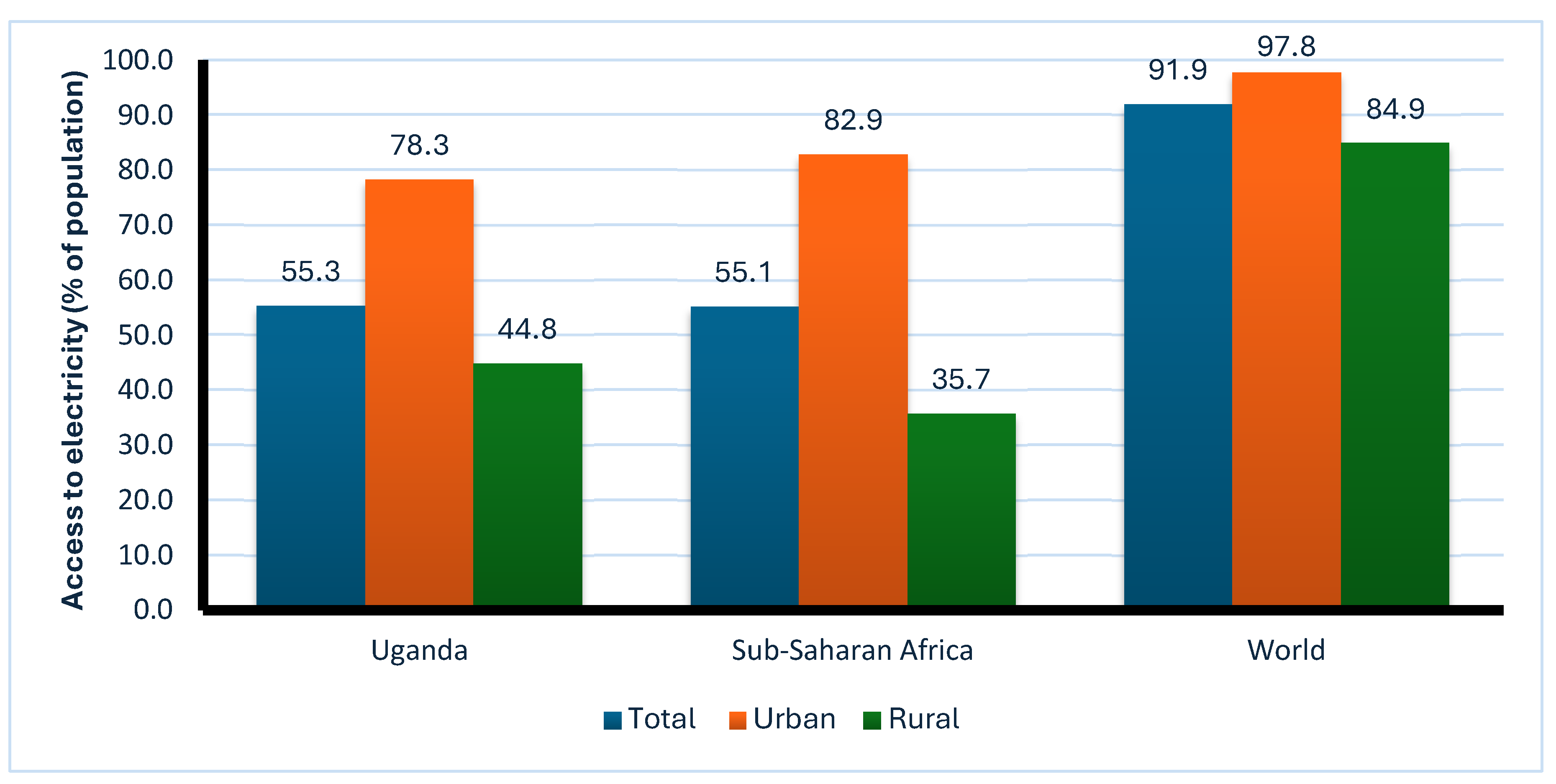
Figure 2.
Distribution of households by principal lighting source. Source. Authors’ construction based on the 2025 household survey data.
Figure 2.
Distribution of households by principal lighting source. Source. Authors’ construction based on the 2025 household survey data.
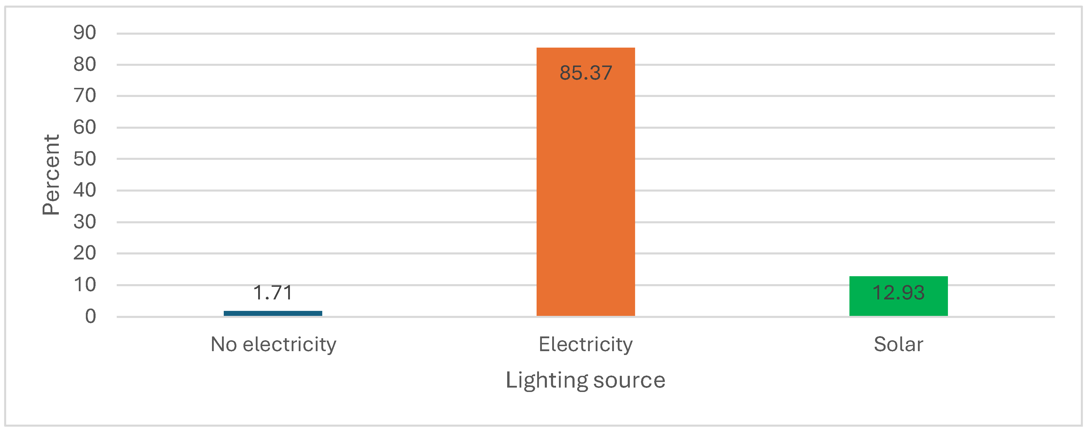
Figure 3.
Average monthly lighting expenditure and efficiency score by study location. Source. Authors’ computation based on the 2025 household survey data. The energy cost label in the graph refers to monthly expenditure on energy used for lighting.
Figure 3.
Average monthly lighting expenditure and efficiency score by study location. Source. Authors’ computation based on the 2025 household survey data. The energy cost label in the graph refers to monthly expenditure on energy used for lighting.
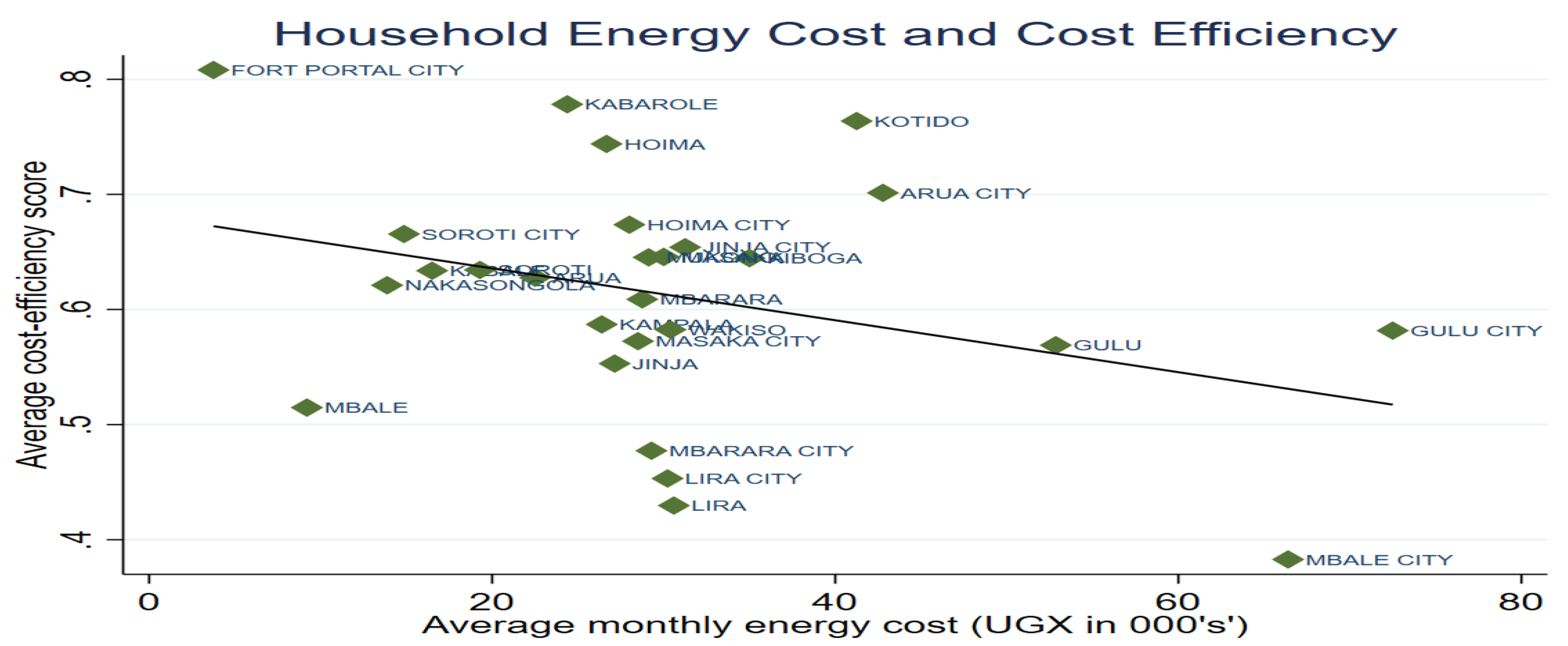
Table 1.
Variable description and measurement.
| Variable name | Description and measurement |
| Lighting expenditure | Monthly expenditure on all energy sources used for lighting, measured in Uganda shillings. |
| Number of rooms | Number of rooms in the household dwelling. |
| Age | Age of the household head in complete years. |
| Location | Household residential location, coded 0 if urban and 1 if rural. |
| Gender | Gender of the household head, coded 0 if male and 1 if female. |
| Housing tenure | Tenure status of the dwelling, coded 0 if owned and 1 if rented. |
| Electricity available hours | Number of hours electricity was available to the household during the last 7 days. |
| Household income | Approximate monthly household income in Uganda shillings, coded 1 if less than 100,000, 2 if 100,000 to 500,000, 3 if 500,001 to 1,000,000 and 4 if above 1,000,0001. |
| Makes mobile payments | Whether the household uses mobile money to make payments over the mobile phone, coded 1 if yes and 0 if no. |
| Energy-efficiency awareness | Whether the household is aware of energy-efficient appliances or practices, coded 1 if yes and 0 if no. |
| Has mobile money | Whether the household has a mobile money account, coded 1 if yes and 0 if no. |
| Education of household head | Highest education level attained by the household head, coded 1 if no education, 2 if primary, 3 if secondary and 4 if post-secondary. |
| Energy-efficiency training | Whether the household head has received energy-efficiency education or training, coded 1 if yes and 0 if no. |
| Household size | Number of household members. |
| Use of energy-efficient appliances | Whether the household uses energy-efficient appliances, such as LED bulbs, coded 1 if yes and 0 if no. |
Source. Authors’ construction based on the 2025 household survey data.
Table 2.
Descriptive statistics.
| Variable | Obs. | Mean | Std. Dev. |
| Monthly lighting expenditure (UGX) | 407 | 14,719.32 (US$3.98) | 15,755.31 (US$4.26) |
| Number of rooms | 410 | 2.72 | 1.79 |
| Age of household head | 410 | 38.76 | 12.65 |
| Location | |||
| Urban | 410 | 0.63 | 0.48 |
| Rural | 410 | 0.37 | 0.48 |
| Gender of household head | |||
| Male | 410 | 0.64 | 0.48 |
| Female | 410 | 0.36 | 0.48 |
| Housing tenure | |||
| Owned | 410 | 0.44 | 0.50 |
| Rented | 410 | 0.56 | 0.50 |
| Electricity availability (hours) | 407 | 21.67 | 22.75 |
| Household income (UGX) | |||
| Less than 100,000 | 410 | 0.08 | 0.27 |
| 100,000 to 500,000 | 410 | 0.50 | 0.50 |
| 500,001 to 1,000,000 | 410 | 0.26 | 0.44 |
| Above 1,000,000 | 410 | 0.16 | 0.37 |
| Makes mobile payments | |||
| No | 410 | 0.05 | 0.23 |
| Yes | 410 | 0.95 | 0.23 |
| Energy-efficiency awareness | |||
| No | 410 | 0.23 | 0.42 |
| Yes | 410 | 0.77 | 0.42 |
| Use of energy-efficient appliances | |||
| No | 410 | 0.50 | 0.50 |
| Yes | 410 | 0.50 | 0.50 |
| Energy-efficiency training | |||
| No | 410 | 0.89 | 0.32 |
| Yes | 410 | 0.11 | 0.32 |
| Education of household head | |||
| No education | 410 | 0.10 | 0.31 |
| Primary | 410 | 0.13 | 0.34 |
| Secondary | 410 | 0.41 | 0.49 |
| Post-secondary | 410 | 0.35 | 0.48 |
| Household size | 410 | 4.53 | 2.65 |
| Has mobile money | |||
| No | 410 | 0.03 | 0.16 |
| Yes | 410 | 0.97 | 0.16 |
Source. Authors’ construction based on the 2025 household survey data. Means for categorical variables are proportions. Monthly lighting expenditure is reported in Uganda shillings, with approximate US dollar equivalents in parentheses.
Table 3.
Stochastic frontier estimates for lighting expenditure.
| Variable | (1) OLS | (2) Frontier |
| Number of rooms (log) | 0.351*** (0.107) | 0.423*** (0.093) |
| Household head age (log) | −0.206 (0.180) | −0.336** (0.167) |
| Location (Rural) | −0.072 (0.099) | −0.182** (0.088) |
| Household head gender (Female) | −0.153 (0.110) | −0.085 (0.087) |
| Housing tenure (Rented) | −0.229 (0.149) | −0.253** (0.113) |
| Electricity available hours | 0.006*** (0.002) | 0.007** (0.003) |
| Household income (reference: less than 100,000) | ||
| 100,000 to 500,000 | −0.277 (0.175) | −0.145 (0.175) |
| 500,001 to 1,000,000 | −0.258 (0.170) | −0.261 (0.185) |
| Above 1,000,000 | −0.632*** (0.183) | −0.645*** (0.203) |
| Mobile payments (Yes) | 0.434** (0.192) | 0.493*** (0.181) |
| Energy-efficiency awareness (Yes) | 0.136 (0.106) | 0.190* (0.103) |
| Constant | 9.603*** (0.727) | 10.474*** (0.671) |
| σu | 0.607*** | |
| σv | 0.604*** | |
| λ = σu/σv | 1.004*** | |
| γ = σu²/(σu² + σv²) | 0.502 | |
| Wald χ² (11) | 82.60*** | |
| Observations | 378 | 378 |
| R-squared | 0.127 | |
Note. Robust standard errors in parentheses. *** p<0.01, ** p<0.05, * p<0.1. The dependent variable is the natural logarithm of monthly lighting expenditure. Urban location, male head, owner-occupied dwelling, income below UGX 100,000, no mobile payments and no awareness are the reference categories. γ is computed from the estimated σu and σv. Source. Authors’ computation based on the 2025 household survey data.
Table 4.
Lighting expenditure, efficiency scores and regional rankings.
| Variable | Mean (UGX) | Mean (US$) |
| Panel A. Frontier sample (N = 378) | ||
| Observed monthly lighting expenditure | 15,848.58 | 4.28 |
| Efficiency score | 0.59 | |
| Efficient frontier expenditure | 11,101.00 | 3.00 |
| Lighting-cost waste | 4,747.58 | 1.28 |
| Panel B. Region | Mean efficiency score | Rank |
| Toro | 0.72 | 1 |
| Central | 0.60 | 2 |
| Ankole | 0.58 | 3 |
| Northern | 0.58 | 4 |
| Eastern | 0.55 | 5 |
Note. All means are computed over the 378 frontier households. Frontier expenditure and waste are the means of Equations 8 and 9 and sum to the mean observed expenditure. The efficiency score is the mean of the household ratios in Equation 7. US dollar values use UGX 3,700 per US$1. Source. Authors’ computation based on the 2025 household survey data.
Table 5.
Linear probability estimates and average marginal effects for energy-efficient appliance adoption.
Table 5.
Linear probability estimates and average marginal effects for energy-efficient appliance adoption.
| Variable | (1) LPM | (2) Logit AME | (3) Probit AME |
| Energy-efficiency awareness (Yes) | 0.399*** (0.050) | 0.396*** (0.051) | 0.395*** (0.049) |
| Energy-efficiency training (Yes) | 0.217*** (0.061) | 0.233*** (0.069) | 0.230*** (0.066) |
| Household income (reference: less than 100,000) | |||
| 100,000 to 500,000 | 0.315*** (0.077) | 0.304*** (0.068) | 0.314*** (0.067) |
| 500,001 to 1,000,000 | 0.410*** (0.083) | 0.387*** (0.074) | 0.397*** (0.074) |
| Above 1,000,000 | 0.178* (0.096) | 0.180** (0.084) | 0.185** (0.083) |
| Household head education (reference: no education) | |||
| Primary | −0.095 (0.078) | −0.072 (0.084) | −0.077 (0.084) |
| Secondary | 0.145** (0.071) | 0.161** (0.075) | 0.165** (0.075) |
| Post-secondary | −0.054 (0.077) | −0.035 (0.080) | −0.025 (0.079) |
| Household head age | 0.004** (0.002) | 0.005** (0.002) | 0.005** (0.002) |
| Household head gender (Female) | 0.060 (0.043) | 0.053 (0.042) | 0.056 (0.042) |
| Household size | 0.020** (0.010) | 0.019** (0.009) | 0.020** (0.009) |
| Location (Rural) | −0.186*** (0.045) | −0.180*** (0.043) | −0.182*** (0.043) |
| Mobile money (Yes) | 0.174** (0.083) | 0.220** (0.104) | 0.226** (0.106) |
| Number of rooms | 0.011 (0.015) | 0.007 (0.014) | 0.006 (0.014) |
| Constant | −0.558*** (0.141) | ||
| Observations | 410 | 410 | 410 |
| R-squared | 0.312 | ||
| Breusch–Pagan χ² | 0.030 | ||
| Ramsey RESET F-stat | 2.100* | ||
Note. Robust standard errors in parentheses. *** p<0.01, ** p<0.05, * p<0.1. The dependent variable equals 1 if the household uses energy-efficient appliances and 0 otherwise. LPM denotes the linear probability model and AME denotes average marginal effects. Income below UGX 100,000, no education, male head, urban location, no awareness, no training and no mobile money account are the reference categories. Source. Authors’ computation based on the 2025 household survey data.
Disclaimer/Publisher’s Note: The statements, opinions and data contained in all publications are solely those of the individual author(s) and contributor(s) and not of MDPI and/or the editor(s). MDPI and/or the editor(s) disclaim responsibility for any injury to people or property resulting from any ideas, methods, instructions or products referred to in the content. |
© 2026 by the authors. Licensee MDPI, Basel, Switzerland. This article is an open access article distributed under the terms and conditions of the Creative Commons Attribution (CC BY) license (http://creativecommons.org/licenses/by/4.0/).
Copyright: This open access article is published under a Creative Commons CC BY 4.0 license, which permit the free download, distribution, and reuse, provided that the author and preprint are cited in any reuse.