
Submitted:
28 October 2026
Posted:
29 October 2026
You are already at the latest version
Abstract
n this study We utilized GPS - based TEC data from four ground based stations: Thule, Greenland and Ny-Alesund, Norway in the Northern hemisphere, and Syogo and Palmer in the Southern Hemisphere. While earlier studies have explored storm-time TEC fluctuations caused by mechanisms such as prompt penetration Electric fields (PPEF), disturbance dynamo effects , and thermospheric composition changes, high-latitude ionospheric behaivor- particularly during this specific storm has received relatively little attention. Furthermore, important irregularities like ploar cap patches and subauroral ion drifts remain underexplored in hemispheric comparisons. This work fills a critical gap by presenting a comparative , high-resolution analysis of Vertical TEC in both hemispheres, integrating key geophysical drivers such as Polar cap index, AE(AL/AU) indices, IMF Bz, and SYM-H. Results reveal distinct hemispheric responses: VTEC peaks at ∼ 19 TECU (Thule), ∼ 10 TECU (Ny-Ålesund), ∼ 21 TECU (Syowa), and ∼ 22 TECU (Palmer), with stronger variability observed in SH stations. These differences are attributed to enhanced solar EUV exposure, hemispheric magnetic field assymetries, and intensified particle precipitation during storm-time electrodynamic conditions. By providing new insights into the dynamics of magnetosphere-ionosphere coupling during geomagnetic storms. This study contributes to a more comprehensive understanding of high-latitude space weather effects and sets the stage for future modeling and monitoring efforts.
Keywords:
ionosphere
; total electron content
; geomagnetic storm
; magnetosphere-ionosphere coupling
; polar cap index
1. Introduction
The ionosphere is the ionized upper layer of the Earth’s atmosphere that ranges about 60-1000 km above the Earth’s surface (Goodman et al. 2006). It contains significant numbers of free electrons and ions that are primarily produced through photoionization. The main source of the ionization in the ionosphere is the solar radiations such as extreme ultra violate (EUV) and X-ray radiations. In addition to photoionization, collisional ionization due to particle precipitation from the magnetosphere is another source of ionization, in particular in the high latitude region (Chapman et al., 1931).
There are many reports on the diurnal, annual and seasonal variabilities in TEC, specifically related to solar and geomagnetic storms at different longitude and latitude sectors ( Warnant and Pottiaux, 2000; D’ujanga, et al., 2013; Zhang M, et al., 2005; Amaechi et al., 2021; Cherniak et al., 2018; Maruyama et al., 2013; Singh et al., 2021;Shinbori et al., 2022; Mohamed et al.,2023; Rajana et al., 2024). These studies showed that the highest values of TEC were observed during the season of equinoxes and intermediate values during the summer solstices, while lowest values were observed during the winter solstices. They further showed that the annual variations depict a semi-annual distribution with higher values around equinoxes and lower values around solstices. Energy emitted from the sun drives the earth’s magnetosphere, thermosphere and ionosphere. The most powerful solar events like Coronal Mass Ejections (CME) are a result of plasma outbursts from active region of the sun (D’ujanga, et al. 2013).
The solar wind energy deposited into the magnetosphere during geomagnetic storms will eventually be dissipated into the ionosphere and thermosphere. Therefore various physical and energy transport processes takes place in the ionosphere (Buonsanto and Fuller-Rowell, 1997). The high latitude electric field can penetrate into mid, low and equatorial ionosphere during a geomagnetic storm causing significant disturbances in ionospheric conditions (Rastogi, et al., 1977). The disturbed ionosphere is manifested as a large increase or depletion of electron density from their normal level. This kind of response of ionosphere to the geomagnetic storms is known as ionospheric storm (Zhang M, et al. 2005). Prikryl et al. (2011) focused on the high-latitude ionospheric effects including GPS phase scintillation and rapid variations in TEC. They found strong asymmetries of the ionospheric response in the Northern and Southern auroral zones. In addition Several recent papers have reviewed the TEC Variation of the space-earth connections over high latitude regions ( D’ujanga et al., 2012, Milan (2015), Shagimuratov et al. 2009) to mention a few.
The important findings from earlier studies emphasize the need for more irregularities studies over high latitude with newer ground and space-based observations as multi-instrument studies were scanty over this region during past geomagnetic storms. Hence, further investigations with more datasets could at least assist in filling the global gap in knowledge caused by the long-time absence of ionospheric instruments over this regions and also help in complementing our understanding of the vTEC variations during storm. Previous studies (Astafyeya et al., 2016; Cherniak et al., 2019; Zakharenkova et al.,& Cherniak , 2018) have expresed storm-time TEC enhancements and depletions associated with prompt penetration electric fields (PPEF), disturbance dynamo effects, and thermo-spheric composition changes. However, storm-time ionospheric irregularities, including polar cap patches (Spicher et al., 2020) and sub-auroral ion drifts or polarization streams (Zou et al., 2017), also play a crucial role in TEC variability , especially at high latitudes.
Although previous works have reported TEC variations during geomagnetic storms, especially at low and mid-latitudes, high latitude regions particularly during the October 2016 storm remain not explored. Limited comparative studies exist that examine both NH and SH responses with adequate temporal resolution. Moreover, few analyses have integrated critical storm-time drivers such as the polar acp index and AE (AU/AL) indices to understand the ionospheric electrodynamics. SO, this study aims to fill this gap by providing a detailed, hemispheric comparison of VTEC variations during this storm, enhancing our understanding of magnetosphere-ionosphere coupling at high latitudes.
2. Materials and Methods
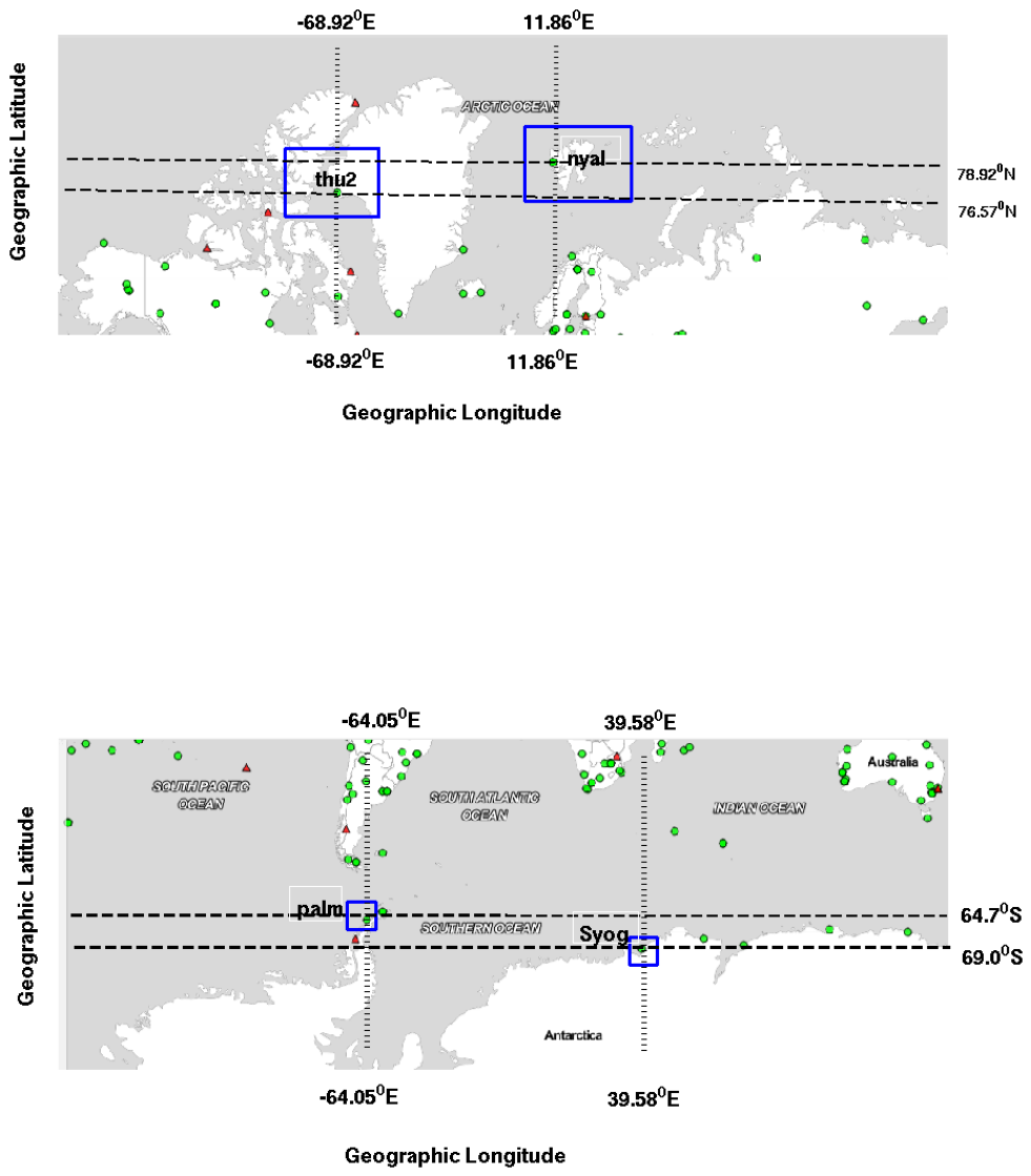
GPS permanent observations carried out over high latitude regions specifically listed in Table 1.
Figure 1.
study Locations by (Google map)
The present study has been carried out with three types of data sets: Ionospheric data (GPS derived TEC), geomagnetic indices (SYM-H, AE, AL/AU), Interplanetary electric field (IEF), Interplanetary magnetic field (IMFBz), speed of solar wind (Vsw) and proton density (Np) from OMNI data base to characterize the magnetic field and Electric field variations, and to determine its impact on TEC variation. The ionization level in the ionosphere is measured by TEC unit (TECU). By Considering the integral of electron density N along a cylindrical column centered on ray path S, between receiver R and satellite S through the ionosphere as shown on Figure 2. The mathematical definition of; TEC is as follows:-
The data at four stations were obtained from the network of GPS receivers that are spread over the globe and the data was recorded periodically. The GPS data recorded by IGS is freely available to all the users and can be downloaded from the URL http://sopac.ucsd.edu. This data is available in RINEX (Receiver Independent Exchange Format); it is an internationally accepted data exchange format. The ionospheric TEC data is processed using Gopi seemala for TEC extraction from RINEX files, and further analyzed using MATLAB for visualization and statistical evaluation. The satellite Differential Code Biases (DCBs) used in TEC computations are obtained from the Center for Orbit Determination in Europe (CODE), maintained by the Astronomical Institute of the University of Bern (AIUB), not from the IGS “code” file as previously indicated. If CODE bias files are unavailable, the software estimates them using its internal algorithms [38].
In practice, slant TEC values, which are measured along the ray path from a GPS satellite to a ground receiver, are converted to equivalent vertical TEC assuming the ionosphere to be compressed into a thin shell at a shell height of h and it is obtained from the slant TEC (STEC) by use of a mapping function (Mannucci et al., 1993). In this study, an elevation cutoff mask of was used for all VTEC computed. Data used to measure TEC Variation during geomagnetic storm and the level of the storm and its impact on WEJ/EEJ have taken four AE, AU, AL and SYM-H indexes. 1 minute values of SYM-H and AE indices were obtained from the World Data Center (WDC) Kyoto, Japan website (http://swdc.kugi.kyoto-u.ac.jp/dstdir). Ey component of the Interplanetary electric field (IEF), plasma speed (Vsw) and proton density (Np) data were obtained of the Goddard Space Flight Center OMNIWeb (https://omniweb.gsfc.nasa.gov). A comprehensive overview of the space-craft orbit and the instrument can be found elsewhere [kokubun et al.,1994].
Moreover, we included in our analysis several geomagnetic indices that represent the dynamics of both magnetospheric and ionospheric current systems, such as the ring current, auroral electrojets, and polar cap convection. Specifically, we used the high-resolution (1-minute) SYM-H index, which characterizes symmetric (SYM) disturbances in the horizontal (H) component of the geomagnetic field caused by variations in the magnetospheric ring current. In addition, the Auroral Electrojet (AE) indices, derived from high-latitude ground-based magnetometer observations, provide a measure of the intensity and variability of the auroral electrojets.
We also considered the Polar Cap (PC) index, which serves as a reliable proxy for monitoring polar cap magnetic activity and high-latitude ionospheric convection driven by solar wind-magnetosphere interactions. The PC index is especially useful in identifying the onset and intensity of geomagnetic storms and substorms at polar latitudes.
3. Results
A magnetic filament in the Sun’s northern hemisphere erupted on October 08, 2016 around 16:00UT hurling a CME into space. The CME with a weak shock arrived at 21:21 UT on October 12, 2016 as observed by Deep Space Climate Observatory (DSCOVR) at L1-point (http://www:spaceweather:com) (Wan, et al., 2018; J. Sun et al.2018). As shown in Figure 3 the storm sudden commencement (SSC) was observed at 21:21 UT on 12, October 2016. Then the SYM-H increased rapidly and reached the maximum value of 25nT at about 23:00 UT. The SYM-H started to decrease at 23:00 UT, and reached about 0 nT at 12 October to 06:00 UT on 13 October. The SYM-H turned negative at 06:00 UT and decreased rapidly. The minimum value (large storm) of SYM-H was about -110nT at about 17:00 UT on 13 October 2016 indicates the main phase of the storm. The main phase lasted for 17 hr. The SYM-H returned and approached to normal after main phase at about 23:00 UT on 13 to 24:00UT 14 October 2016.
Figure 3(a), shows that on 13 October 2016 the geomagnetic indices is more in intense value. Auroral geomagnetic activity indices AE, AL and AU values shows an intense global electrojet activity in the auroral zone during the main phase on 13, October 2016 of the storm’s day. The maximum amplitude of AL=-1300nT (around 13:00 UT and again after 03:00hr at 17:00 UT) around (AL= -2000nT) of 13, October 2016 represents the maximum perturbation generated by Westward electro jet current in the dusk and pre midnight sector respectively over high latitude regions. The difference between AU-AL gives the AE index which used to monitor the magnetic signature (intensity of magnetic field) of the eastward and westward auroral electrojets in the Northern and southern hemispheres (Liu, et.al 2010). At the higher latitudes, Auroral Electrojet (AE) currents transfer energy in the form of heat, by the physical process of Joule heating, which is one of the important energy inputs into the Earth’s ionosphere along with extreme ultraviolet radiation and charged particle precipitation, to the neutral gas.
Thus, during the main phase of the geomagnetic storm (at 06:00 UT to 23:00 UT) of 13, October, 2016 the auroral region, as monitored in terms of the AE index, is characterized by an intense storm activity in both hemispheres. This variations shows that there is the geomagnetic storm occurred on October 13, 2016 has been capable to increase the intensity of the various electric current systems owing in the magnetosphere and ionosphere activating a chain of processes which cover a wide range of time and spatial scales and, at the same time, to activate strong interactions between magnetosphere and ionosphere.
Figure 3(b) shows the decrease in Sym-H value is due to southward IMF(Bz < 0)[Tsurutani et al.,1988]. Using the above definition the minimum Sym-H excursion around (-110 nT) occurred about 17:00 UT on 13th October 2016 can be associated with southward turning of IMFBz reaching -20nT at 17:00 UT; during this periods of IMFBz magnetospheric electric fields can penetrate to the ionosphere (Wagwan, et al., 2010). These penetration electric fields can have a significant impact on ionospheric TEC. This decrease occurs because geomagnetic storms are generally associated with a southward interplanetary magnetic field, which allows for an efficient energy coupling of the solar wind and magnetosphere-ionosphere interaction. The net result is an intensification of the ring current, which is the westward current that encircles the Earth at high latitudes. The enhanced westward current (AL=-2000nT of 13, October, 2016) accounts for the negative Sym-H during the main phase of a storm. Following the initial phase on 12, October 2016; the main phase had been unfolding under southward Bz orientation; when a reconnections or coupling of geomagnetic storms with the geomagnetic field is produced, which results in a large amount of energy deposition in to the high latitude regions of the earth; on 13 October 2016. The Sym-H indice summarizes the north-south magnetic perturbations measured by a longitudinal network of high latitude magnetometers, and are sensitive to the magnitude of the ring current ( Liu, et.al 2010).
Figure 3(e) shows that Interplanetary electric field (IEF(Ey)) component started fluctuating but pointed northward several hours during the main phase, from about 06:00UT to 23:00 UT on 13, October 2016, and then turned south (negative). But the IMFBz component turned negative (southward) from about 06:00 UT to 23:00 UT on 13, October 2016, and practically fluctuate around during several hours after that. The long duration of Bz in southward direction indicated magnetic reconnection for a significant length of time. The solar wind speed (Vsw) and the proton density Np abruptly increased from about 300 to 450 km/s and from 5 to 35 at 00:00 UT to 06:00 UT on the storm day, both decaying during the main phase. A second enhancement was observed in Np during the recovery phase, about 10:00UT on October 14 . Now we can consider from Figure 3(e) this , since it is directly connected to the energy, mass and momentum transfers from the interplanetary space to the near-Earth electromagnetic environment[Gonzalez et.al, 1999]. Indeed, when Bz is southward oriented, solar wind particles are favorite to enter the magnetosphere via magnetic reconnection at the flanks of it, while when M-I coupling function increases this means that a huge amount of energy is transferred to the magnetosphere that rises VTEC variations over high latitude regions.
Therefore the variations of interplanetary magnetic field () and interplanetary electric field (IEF) during 12-14th October 2016 shows that there is excellent inversely correlation between Interplanetary magnetic field and Interplanetary electric field (IEF). Hence the coronal mass ejection (CME) from polar cusp is includes a high energetic particles that can affect other interplanetary fields or other solar wind parameters such as Interplanetary electric field and Interplanetary magnetic field. The Interplanetary electric field is turned north and Interplanetary magnetic field was turned South. This enhances the geomagnetic storm and turn in the main phase, interrupt the communication, block the signal, navigation system, makes error in GPS measurement and vary VTEC around the receivers. After the recovery phase the Sym-H was almost constant and appear as quit time and around zero unit in measurement. Starting from initial point the interplanetary electric field moves from zero to south of direction and interplanetary magnetic field is moves to the north direction and vice versa.
The first peak of AE that was observed on October 13, 2016 at 08:00UT is due to the CME-induced storm while the second peak which was observed on October 13, 2016 at 17:00 UT to 17:30 UT is due to the CIR related magnetic storm (Koskinen et al., 2011). The AE index remained above around 2000nT for about 30 min during 17:00 UT to 17:30 UT on October 13, 2016. The significant enhancements of AE-index are an indication of heating energy source at high latitude which has been generated during this geomagnetic storm may lead to generation of disturbance dynamo electric field (DDEF). It should also be noted that the positive storm effect observed for the CME induced storm was less significant than that observed during the CIR induced storm on October 13. This is due to the fact that the onset of the storm at 23:00 UT on October 12 was not in the morning to noon sector in which the ionization production mechanism dominates and plasma accumulation due to mechanical effect of neutral wind is greater than its chemical loss due to recombination (Ray et al., 2017).
Again returning to Figure 3 and comparing the auroral electrojet indices AU and AL (Figure 3a) with Sym-H in Figure 3.b, we note that periods of enhanced solar wind driving and R1/R2 currents are also periods of enhanced electrojet activity (B. Sonnerup, et al. 1974). The two highlighted events with the largest peaks in (AE=2000nT) at 17:00UT (around pre midnight), are accompanied by negative excursions in Sym-H (about -110nT) at the same time, storm main phases, indicating enhancement of the magnitude of the ring current by M-I coupling process. The occurrence of spikes in the solar wind density ( Minimum TEC starting around 21:21 UT on 12, October 2016 from Figure 3.b), produce positive excursions in Sym-H, storm initial phases, associated with enhanced and inwardly compressed magnetopause currents. This indicates that the FAC generated at the high latitude regions are closed through AE.
As shown Figure 4 above polar cap index in the NH starts from 12, October 2016 about 18:00-22:00 UT , PCN remained low (∼ 0.5 - 1.5 ) but at ∼ 23:00 UT , a sudden increase in to ∼ 5 indicated the SSC. Between 00:00-6:00 of 13, October, PCN rose rapidly to reaching ∼ 12-15 as turned strongly southward (∼ -10 nT) leading to enhanced magnetospheric convection. Peak PCN occured around 04:30-05:30 with values exceeding 18 , later from 06:00-12:00 , PCN remained elevated (∼ 12-16 ) , tracking sustained polar cap convection. This means the electric current across the polar ionosphere is quite strong, indicating active coupling between solar wind and Earth’s Ionosphere polar ionosphere , typically during the main phase of a geomagnetic storm [36,37]. For SH at 12,October 2016 PCS values were stable and low 1-2 until ∼ 23:00 but SSC observed with PCS rising to ∼ 4-5 between 23:00 -00:00UT,then at 13, October main phase grows up between 00:00-03:00 , PCS increase to ∼ 4-5 and peak is occured between 03:00 -06:00 with maximum near 12-14 . Here PCS was slightly lower and more variable than PCN throughout the main phase.
4. Discussion
4.1. Diurnal Variation of TEC During Storm over High Latitude Regions
The diurnal TEC variation over the auroral and sub- auroral zone stations over high regions for both NH and SH , daily TEC was analyzed for every hours of 12-14, October 2016 at a sampling interval of 1 minute. This interval provided sufficient information to monitor the changes in daily TEC. Diurnal for Northern regions told us TEC for three days of the 12-14, October 2016 is presented in the Figure 4 ( a and b) for Northern hemisphere Thule and Ny-Alesund stations at high latitude . This figures indicates the variation of TEC for three storm days (12-14, October 2016) of the month and one quiet day (11, October 2016) for both Thule and Ny-Alesund stations respectively. From this plots, we may observed that the maximum TEC (19 TECU, highest peak of green line at 17:50 UT (LT= UT-4hr=12:50 hr)) and (10 TECU, highest peak of green line nearly at 21:00 UT (LT=22hr)) during 13 October 2016 over Greenland and Norway respectively were obtained during the same day at 24:00UT Over NH of high latitude regions.
A peak in VTEC at 17:50 UT (LT=12:50hr) over Denmark could be attributed to the daytime photo-ionization, due to solar EUV and x-ray radiation in addition to the storm. But 21:00UT (LT=22:00hr) over Norway was attributed to night time ionization, which must be due to collisional ionization due to charged particle precipitation from the magnetosphere during the storm. Because Ion-neutral collisions are a significant source of ion heating at high latitudes. Therefore, these studies suggested that the nighttime enhancement in TEC is associated with the electrodynamic drifts, plasma motion due to neutral wind and westward directed electric field during the post-sunset hours which accomplished a downward E X B drift motion. But for Southern hemisphere that Figure 5(c) and (d) shows that the TEC variation occurrence over Syogo and Palmer stations located near the poleward edge of the auroral oval, which the optical emissions that are a result of the energy from precipitating energetic particles (mostly electrons) being deposited in the ionosphere. The behavior of the variations at both stations is rather similar. The TEC variations were observed even in the quiet period (11, October 2016). During the most disturbed day of 13, October 2016, the intensity of variations increased and was variable during the entire day.
The development of the TEC variation over the sub-auroral stations is also controlled by the behavior of Bz specifically for SH (see Figure 3(e)), and the variations were maximal (21 TECu at 11:45UT (LT=14:15hr)) when Bz was extremely negative (around -18nT at 11:00UT (13:30 LT)) over Syogo station. At local daytime, the enhancement in TEC is mostly due to the increased IMF values. Thus during periods with Bz orientation, Joule heating is more prevalent around the night side sub-auroral zone. At 21:45UT (LT=UT-4hr=17:45hr), at the palmer station, maximum TEC (22TECU) variations were expressed when Bz fluctuates its sign around -15nT as shown in Figure 3(c). Therefore the enhancement in TEC might be charged particle precipitations from the magnetosphere. This time delayed might be the differences of longitude or latitude between two stations and it might be due to storm of ionospheric traveling disturbance.
Generally, as shown in above Figures 4 and 5 during disturbances, the VTEC variations was much higher at the southern stations Syog and Palmer than at Northern stations NYAL and Thule; because of long time (about 17 hrs) turning of IMFBz toward southward, and larger daily variation in solar illumination, are likely to produce larger diurnal variations in geomagnetic activity in the SH compared to the NH (which matched with Prolls et al., 1991). Day-by-day development of VTEC variations at these stations shows some similarities and differences. During the disturbed days, when Bz was negative, strong variations prevailed over southern hemisphere. Therefore, the results also shows that even if the peak VTEC value is vary from hour to hour or from day to day, noon hour TEC is synchronously moving westward in all the selected days of the September equinox month. The results of the four stations also shows that ionospheric VTEC is Maximum at night time, at the time where many more particles descend in the night part of the earth, causing frequent auroras. This explains the higher VTEC values observed at night. But the difference of time was observed because of local time and latitudinal or longitudinal differences of the stations location. The mean VTEC presents stronger solar activity sensitivity at southern hemisphere than Northern hemisphere over high latitude regions (Prolls et al., 1991).
4.2. Effects of Geomagnetic Storm Parameters on Spatial Variation of vTEC over High Latitude Regions
The variations in daily VTEC for both selected stations of NH are investigated during the geomagnetic storm recorded on October 13, 2016. To monitor the short term effects of this storm on the behavior of VTEC, we have selected three days (i.e. 12-14 October) including the storm day. The VTEC is shown in the context of solar and geomagnetic storm indices which are represented from AE index, SYM-H index, Interplanetary magnetic field IMF-Bz, solar wind speed (Vsw) and Interplanetary electric field IEF(Ey)(see Figure 3).
The value of IMF(Bz) on October 12, 2016 until 21:21UT lies in between -5 nT to 5nT (Figure 6). Similarly, the AE, Vsw, Np, Electric field and SYM-H index is around 0nT, 350km/s - 400 km/s, 8 , around 2mV and 0nT, respectively. IMFBz fluctuated south and North at the time of SSC with corresponding fluctuations in IEF(Ey) from westward to eastward till 23:00 UT on 12, October 2016. The solar wind Vsw raised up from about 350 km/s at about 23:00 UT on 12 October to almost 450 km/s around 06:00 UT of the next day on October 13, 2016. It shows the commencement of the initial phase of the geomagnetic storm at 06:00UT on October 13, 2016 (see Figure 3).
The symmetric horizontal index was the most parameter which used to determine the level of geomagnetic storm. Each southward turning was associated with an increase in convection electric field as well as enhanced auroral elecrojet ( M. Sugiura,1991). Therefore as shown in Figure 3(b and d) there is almost the inverse relationship between TEC and symmetric horizontal index. During 13 October 2016 the TEC lasts North pole around 00:30 min (17:30 to 18:00 UT (LT=12:30-13:00hr) over Denmark) and around 01:00hr (21:00 to 22:00 UT (LT=22:00hr-23:00 hr) over Norway) and the symmetric horizontal index Sym-H lasts South pole for similar time for both stations. This relation explains that the disturbance of symmetric horizontal index Sym-H is a significant effect to disturb the vTEC measurement and enhances magnetic reconnection’s due to the magnetosphere-ionosphere stormy condition in high latitude regions.
The figure shows that the auroral geomagnetic activity indices AE, AL and AU which is in an intense global electrojet activity in the auroral zone during both the main phase and the recovery phase of the storm’s day; Figure 3b-e) shows that the SYM-H, Np , Vsw , and from (e) the red color IMFBz and green indicates IEF (Ey) respectively. Red line found in Figure 3f) shows that the VTEC over Syogo station, blue line found on figure shows that the variation of TEC due to storm for Palmer Antarctica stations. The main phase of the storm day started on October 13th at 06:00UT which leads to the minimum value of SYM-H(-110nT) at 17:00UT, which is also an intense storm and the recovery phase started on October 13th with SYM-H value -100 nT at 24:00UT. This interrelate the effects of interplanetary magnetic field IMFBz on VTEC over SH. Highly rising of negative interplanetary magnetic field IMFBz (-20nT) around 17:00UT can lead maximum increment of VTEC about 21TECU at 12:00UT and 22TECU at 22:00UT over syogo and palmer stations respectively. Because, Interplanetary magnetic field IMFBz and the earth’s magnetic field interact each other and enhanced the VTEC value on the high latitude region over SH.
Finally the perturbation of interplanetary magnetic field IMFBz causes the stormy condition of the M-I through variation of VTEC over SH. Another is the relation between the VTEC over SH and symmetric horizontal index found on Figure 4.5 (b and f). As shown in figure there is almost the inverse relationship between VTEC and symmetric horizontal index. During 13 October 2016 the VTEC lasts North Pole around 02:00UT (09:30 to 11:30 UT over Syogo East Ogleo Island and around 00:30min (22:30 to 23:00 UT over Palmer Antarctica) and the symmetric horizontal index Sym-H lasts south pole for similar time for both stations. This relation shows that the disturbance of symmetric horizontal index Sym-H is a significant effect to disturb the VTEC measurement over southern hemisphere and makes the magnetosphere-ionosphere stormy condition in high latitude.
The source of the storm is CME driven geomagnetic storm since all the indicators such as the interplanetary magnetic field (IMF(Bz)) is directed southward implies reconnection with the magnetic field; as a result magnetic field is reduced at the main phase, so that voltage is induced the change in magnetic field in the magnetosphere induces current to oppose the change in flux in the magnetosphere. In this main phase of the storm, the enhancement in VTEC could be due to the southward movement of the interplanetary magnetic field, which produces loading of interplanetary particles in the magnetosphere-ionosphere (Kumar and Singh 2010). In the recovery phase, the enhancement was due to the upward drift of the southward IMF-Bz during local post-midnight hours (i.e, downward EXB plasma drift) (Balan et al. 2013).
Generally the magnitude of the VTEC variation is much larger in the midnight sector than in the morning time enhancement and also as compared to the enhancement during the 13 October 2016 storm. Because, Auroras appear when high-energy particles coming from the Sun and traveling at high speed along the geomagnetic force lines finally enter and collide with the outermost layers of the atmosphere of the Earth (Zeilik et al., 1992). Especially, many more particles descend in the night part of the Earth, causing frequent auroras. This explains the higher TEC values observed at night.
4.3. Comparison of VTEC Variation Between Northern and Southern Hemispheres
Figure 4.6 (a) the red line indicates the VTEC over Denmark, the blue line indicates VTEC over Norway and, Figure 4.6 (b) indicates the red line the VTEC over Syogo Island, the blue line indicate VTEC over Palmer Antarctica.
In the VTEC time series plot in Figure 3.6a) we see that the TEC increases and fluctuates from early morning until pre midnight and peaks around 21:00 UT (LT=22 hr) for Ny-Alesund station of Norway. The peak propagates Northwards with time and the VTEC reaches a maximum of 10 TECU at local morning time. But for Thule station the VTEC decreases and vary from midnight until 11:00UT (06:00LT local early morning) and after this time it is increasing dramatically peaks around 17:50UT (12:50LT local post midday) reached maximum TEC of 19TECU. To describe the VTEC variation for the storm of 13th October 2016 over Southern hemisphere; as shown in Figure 3.6(b) the VTEC increases from early morning until afternoon and peaks (20TECU) around 11:45UT (13:45LT) (near to dusk) for Syogo station of Ogleo Island Antarctica and decreased with small scale fluctuation to (below 8TECU) at night time starting from 12:00 UT (14:30LT) to 24:00UT (02:30LT) of 13, October 2016. But for Palmer station the VTEC decreases and fluctuate from early morning until post midday (08:30 UT (04:30 LT)) and by increasing simultaneously peaks around 21:50 UT (17:50LT) (near to dusk) reached maximum TEC of 22TECU and again falls to 0 TECU around 06:00UT of 14, October 2016.
Generally as shown in Figure 3.6; the VTEC variations occurrence over Thule and NYAL from NH stations and, Syogo and palmer from SH stations located near the pole ward edge of the auroral oval. The behavior of the variations at both hemispheres stations is rather similar. The TEC variations were observed even in the quiet period (as at the polar stations). During the most disturbed day, the intensity of fluctuations increased and was variable during the entire day. The development of the TEC variations over the auroral stations is also controlled by the behavior of Bz. At the same time, at the Syogo and Thule stations, VTEC variations were very well expressed when Bz sharply changed its sign to North-South.
As shown in Figure 3.6) during disturbances, the TEC Variation was much higher at the southern stations than at Northern stations was because of North-South asymmetry in the magnetic field, together with variations in the Sun-Earth distance, result in the SH high latitude ionosphere experiencing greater exposure to EUV radiation compared to the NH enhances more VTEC variation over SH than NH and due to arrival of the geomagnetic storm. Hence the southward migration of the VTEC maximum (22 TECU and 21 TECu) from Figure 3.6b) at 21:50 UT and 11:50 UT could imply that either is the ionization due to M-I coupling was strongest in Palmer and syogo stations of SH, or an expanded auroral oval with associated irregularity zone [Aarons et al.,1997] migrates equator wards with the reconnection processes caused by the geomagnetic storm. The increased TEC in Southern hemisphere at post-midnight over Palmer station and Midday over Syogo station registered at 21:50 UT and 12:00 UT respectively, are indeed coinciding with the onset of expansion phases in the AL-index in Figure 4.4b). The increased VTEC of 19TECU in Denmark at approximately 17:50 UT, is due to the patch material from the TOI. It is unusual to record such high TEC values in the evening unless there are EUV-plasma patches that have drifted across the PC from the dayside involved [Jacobsen et al., 2014]. Apart from the peaks in the midday and evening, the VTEC decreases to 8TECU in the afternoon.
4.4. TEC Asymmetries at High Latitudes
At F-region altitudes, production and loss of ions and electrons are governed by solar EUV radiation along with the thermosphere composition (Weygand et al. 2014). In particular, photoionization of atomic oxygen (O) is the primary source of O+, which dominates the F-region plasma population. The loss of O+ is due to ion exchange reactions with molecular nitrogen (N2) and molecular oxygen (). Spatial and temporal variability in either the EUV radiation or thermosphere composition will therefore have a direct impact on the F-region electron density. Asymmetries between the geomagnetic field in the Northern and Southern hemispheres introduce an asymmetry in the solar EUV radiation and the neutral composition, leading to hemispheric differences in the F-region electron density (Zhao et al. 2014; K.M. Laundal et al., 2016). This is primarily due to the offset between the magnetic and geographic poles.
From our analysis of Figure 1f PCN is consistently showed higher values than PCS. Asymmetries due to different sunlight condition (Northern polar nights versus Southern spring) , station geometry and ionospheric conductivity can result to Hemispheric asymmetry. So, the NH showed stronger and longer lasting responses than the southern , a common observation during this time of year. As shown in Figure 3.6 (a and b) above, there was VTEC Variation differences in the solar illumination of high magnetic latitudes in the Northern and Southern hemispheres. North-South asymmetry in the magnetic field, together with variations in the Sun-Earth distance, result in the SH high latitude ionosphere experiencing greater exposure to EUV radiation compared to the NH. Additionally, an energy input at high latitudes and changes in the (horizontal and vertical) transport modifies [O/N2]. As the energy input is related to the geomagnetic field geometry, the thermosphere composition, and its impact on production and loss of ions and electrons, will be impacted by hemispheric asymmetries in the geomagnetic field (Anthes et al. 2008).
In general, the higher VTEC variations took place when the Bz component was southward [Shagimuratov, et al., 2012]. However, VTEC variations were observed when Bz turned northward or varied around zero at 12, October , which occurred prior to the storm onset in 2016. It is well known that geomagnetic storms are triggered by impulsive changes in parameters of the solar wind parameters (Proton density, speed, and pressure). The increased solar wind compresses the Earth’s magnetosphere, and when the component Bz is negative (southward) a reconnection or coupling with the geomagnetic field is produced, which results in a large amount of energy deposition into the high latitude regions of the Earth [Gonzales,et al., 1994].
Such high latitude heating, in turn, create strong prompt penetration electric fields (PPEFs), which appear almost immediately in the Earth’s ionosphere and magnetosphere after they have been converted to the magnetosphere by the disturbed solar wind. The PPEFs are directed eastward (dawn to dusk) on the dayside and westward (dusk to dawn) on the nightside. A feature of these high-latitude electric fields is that they may penetrate to lower latitudes before the ring current has developed. At high latitudes, these intense electric fields produce horizontal plasma convection because the magnetic field lines are near perpendicular to the Earth’s surface. Therefore, the storm-time induced electric fields do not produce vertical drifts, but there is a vertical component where the magnetic field is tilted a little from the vertical.
4.5. Geomagnetic Storm and Electrodynamics Events of 13, October 2016
Figures 4.4 a-e illustrate time series of solar wind parameters, Interplanetary fields and VTEC constructed for the time period of 00:00 UT 12 October to 24:00 UT 14, October 2016 for both hemisphere. On 12 October, the sudden storm commencement (SSC) occurred at 21:21UT of 12, October 2016. The following initial phase (23:00-06:00UT of 13, October 2016) and main phase (06:00-23:00 UT of 13,October 2016) at when SYM-H reached its minimum value of -110nT and thus registered the onset of the recovery phase at 24:00UT of 13, October 2016. However, this recovery phase unfolded under southward Bz conditions. The magnetospheric electric field is carried along the Region-1 field-aligned current (R-1 FAC) and transmitted to the polar ionosphere by Alfven waves [Southwood and Kivelson, 1991]. The R-1 FAC flows downward (owing into the ionosphere) on the dawn side and upward on the dusk side, and is distributed on the higher latitude side of the auroral zone [Iijima and Potemra, 1976]. The electric field applied to the ionosphere drives the plasma convection in the polar ionosphere by the E drift, while simultaneously generating a twin-vortex Hall current centered on the foot of the R-1 FAC. This is referred to as the DP2 electric current system [Nishida et al., 1966]. Since the Hall current corresponds to the Edrift of electrons in the ionospheric E region, the DP2 current will flow in the direction opposite to the plasma convection of ionospheric F region and will have the same pattern, if the ionospheric electric conductivity is uniform over the polar region. The electromagnetic energy produced in the dayside magnetosphere flows into the polar ionosphere via the R-1 FACs. The resultant electric field causes the development of the two-cell Hall current and plasma convection.
The magnetospheric convection electric field propagates instantly with a precision of several tens of seconds to the global ionosphere and induces the DP2 current at the dayside equator that connects R-1 FAC [Kikuchi et al., 1996]. During the development stage of the convection caused by the southward turning of the IMF, the DP2 convection electric field propagates from the pole to the equator or from the dayside to the night side in the ionosphere within several tens of seconds [Kikuchi et al., 1996]. The above results indicate that the magnetosphere and the ionosphere become coupled by the field-aligned currents, and that plasma convection and DP2 currents are generated in the surrounding the field- aligned currents. The field-aligned currents are mainly controlled by the direction of the IMF Bz. When the IMF turns from northward to southward, R-1 FACs begin to develop, which in turn cause the development of the DP2 current in the global ionosphere including the equator. The convection electric field, which is propagated to the polar ionosphere from the magnetosphere by Alfven waves along the magnetic field lines, is carried to the middle-to-high latitude regions, and this horizontal propagation permits the transmission of energy to the entire magnetosphere-ionosphere coupling system. In this way, the ionosphere plays an important role as the energy transmission path within the entire magnetosphere- ionosphere coupling system.
From Figure 4.4e, we can see that the IMF(Bz) is southward directed, for example, around -20nT at around 17:00 UT of 13, October 2016. The southward directed Bz allows easy entrance for charged particles to the Earth’s magnetosphere which causes auroral activity (Lemaire,2001). When IMFBz component decreases to -20 nT by the time AE index increases to the value around 2000nT. The value of SYM-H index starts to decrease from normal level before 10:00 UT but its value gradually decreases below and reaches to lowest value about -110 nT. This value is sufficient for a storm to occur. For a storm to occur the SYM-H must be <-50 nT (Gonzalez et al., 1994). As the strength of geomagnetic disturbance increases indicated by increase in negative value of SYM-H.
5. Conclusions
This work presents the TEC variation over high latitude regions during storm main phase of geomagnetic storm occurred on 13 October 2016. The SSC was observed at 21:21 UT on 12 October 2016. Then the SYM-H increased rapidly and reached the maximum value at about 23:00 UT. The initial phase was from 23:00 UT on 12 October to 06:00 UT on 13 October. The main phase (06:00 to 23:00 UT of 13, October 2016) lasted for 17 hr. For 13th, October 2016 storm case, the Sym-H index drop to minimum value of -110 nT, when the negative peak of SYM-H registered during this storms, the generation of VTEC variation were found to be enhanced.
The results show that the maximum TEC variation is occurred in Norway (Ny-Alesund ) at 21:00UT and Denmark (Thule) at 17:30UT were around 10TECu and 19TECu respectively. On the other hand, the maximum TEC variation observed in Palmer Antarctica at 22:00UT(18:00LT) and Syogo station at 12:OOUT (14:00 LT), was around 22 TECU and 21 TECU respectively. From this observation we can see that the variation of TEC was much higher at the southern station Syogo and Palmer than at Northern stations NYAL and Thule during geomagnetic disturbances. Because larger daily and seasonal variation in solar illumination, are likely to produce larger diurnal and seasonal variations in geomagnetic activity in the SH compared to the NH.
A peak in TEC at diffeerent time for all stations are therefore must be due to the photoionization due to solar EUV radiation or it is night time ion-electron (frictional) collisional ionization due to charged particles precipitation. The observation also see that, when the latitude is increase the TEC variation decrease. Additionally, the variabilities in the occurrence of TEC variation during storm periods might be explained in relation with AE indeces and solar wind parameters. During the main phase of the geomagnetic storm of 13, October the auroral and sub-auroral region, as monitored in terms of the AE index, is characterized by an intense storm activity in NH and SH. This variations shows that there is the geomagnetic storm occurred has been capable to increase the intensity of the various electric current systems owing in the magnetosphere and ionosphere activating a chain of processes which cover a wide range of time and spatial scales and, at the same time, to activate strong interactions between solar wind- magnetosphere- ionosphere. When Bz is sharply southward oriented , solar wind particles are favorite to enter the magnetosphere via magnetic reconnection at the flanks of it, while when M-I coupling function increases this means that a huge amount of energy is transferred to the magnetosphere that rises TEC variations over high latitude regions.
Author Contributions
Conceptualization, B.D.Z., A.O.G. and A.M.T.; Methodology, B.D.Z., A.O.G. and A.M.T.; Software, B.D.Z., A.O.G. and A.M.T.; Formal analysis, B.D.Z.; Investigation, B.D.Z., A.O.G. and A.M.T.; Data curation, B.D.Z., A.O.G. and A.M.T.; Writing—original draft, B.D.Z.; Writing—review & editing, B.D.Z., A.O.G. and A.M.T.; Visualization, B.D.Z. All authors have read and agreed to the published version of the manuscript.
Funding
This research received no external funding.
Institutional Review Board Statement
Not applicable.
Informed Consent Statement
Not applicable.
Data Availability Statement
The datasets used and/or analyzed during the current study are available from the corresponding author on reasonable request.
Acknowledgments
The author would like to thank the data providers, including the NASA OMNIWeb database and the IGS (International GNSS Service) for making the solar wind and ionospheric TEC data freely available. During the preparation of this manuscript, the author used ChatGPT (GPT-5, OpenAI, 2025) for language editing suggestions. The author has reviewed and edited all AI-generated output and takes full responsibility for the content of this publication.
Conflicts of Interest
The author declares no conflict of interest.
References
- Astafyeva E, Zakharenkova I, Alken P. Prompt penetration electric fields and the extreme topside ionospheric response to the June 2015 geomagnetic storm. J Geophys Res Space Phys. 2016;121(5):5088–5100. [CrossRef]
- Cherniak I, Zakharenkova I, Redmon RJ. Dynamics of the high-latitude ionospheric irregularities during the 7–8 September 2017 geomagnetic storm. Space Weather. 2019;17(1):106–118. [CrossRef]
- Zakharenkova I, Cherniak I. Ionospheric response to the 2015 St. Patrick’s Day storm: TEC and scintillation analysis. J Geophys Res Space Phys. 2018;123(2):2011–2027. [CrossRef]
- Spicher A, Miloch WJ, Clausen LBN, Moen J. Observation of polar cap patches and associated density gradients with Swarm. J Geophys Res Space Phys. 2020;125(2):e2019JA027608. [CrossRef]
- Zou S, Ruohoniemi JM, Wang CP, Zhang XX, Lyons LR, Baker JBH. Formation and evolution of subauroral polarization streams (SAPS): A review. J Atmos Sol Terr Phys. 2017;154:40–53. [CrossRef]
- Coster AJ, Erickson PJ, Rideout W. Storm-time ionospheric irregularities: GPS TEC and scintillation. AGU Fall Meeting Abstracts. 2017;SA13A-2456.
- Hanslmeier A. The Sun and Space Weather. 2nd ed. Graz: University of Graz, Institute of Physics/IGAM; 2007.
- Astafyeva E, Zakharenkova I, Huba JD, Doornbos E, Van den IJssel J. Global ionospheric and thermospheric effects of the June 2015 geomagnetic disturbances: Multi-instrumental observations and modeling. J Geophys Res Space Phys. 2017;122(11):11716–11742.
- Komjathy A. Global Ionospheric Total Electron Content Mapping Using the Global Positioning System [PhD dissertation]. University of New Brunswick, Canada; 1997.
- Balan N, Otsuka Y, Nishioka M, Liu J, Bailey G. Physical mechanisms of the ionospheric storms at equatorial and higher latitudes during the recovery phase of geomagnetic storms. J Geophys Res Space Phys. 2013;118:2660–2669.
- Baumjohann W, Treumann R. Basic Space Plasma Physics. London: Imperial College Press; 2009.
- Bhattarai S, Lopez R. Reduction of viscous potential for northward interplanetary magnetic field as seen in the LFM simulation. [Unpublished].
- Sonnerup BUO. Magnetopause reconnection rate. J Geophys Res. 1974;79:1546–1549.
- Buonsanto MJ, Fuller-Rowell TJ. Strides made in understanding space weather at Earth. Eos Trans AGU. 1997;78(1):1–7.
- Chapman S, Ferraro VCA. A new theory of magnetic storms. Terr Magn Atmos Electr. 1931;36(2):77–97.
- Chapman S, Bartels J. The absorption and dissociative or ionizing effect of monochromatic radiation in an atmosphere on a rotating Earth. Proc Phys Soc. 1940;43:26.
- Costa Jr E, Simoes FJR, Cardoso FR, Alves MV. Solar wind and geomagnetic activity. Rev Bras Ensino Fis. 2011;33(4):4301.
- Costa Jr E, Simoes FJR, Cardoso FR, Alves MV. Alfven waves in interplanetary space. Rev Bras Ensino Fis. 2011;33(2):2302.
- Cowley S. Magnetosphere-ionosphere interactions: A tutorial review. In: Ohtani S, Fujii R, Hesse M, Lysak RL, editors. Magnetospheric Current Systems. Geophys Monogr Ser. 2000;118:91–106.
- Dungey JW. Interplanetary magnetic field and the auroral zones. Phys Rev Lett. 1961;6(2):47–48. [CrossRef]
- Goodman JM. Space Weather and Telecommunications. Springer; 2006. [CrossRef]
- Gonzalez W, Joselyn J, Kamide Y, et al. What is a geomagnetic storm? J Geophys Res Space Phys. 1994;99:5771–5792. [CrossRef]
- Hargreaves JK. The Solar-Terrestrial Environment. Cambridge: Cambridge Univ. Press; 1992.
- Hernandez-Pajares M, Juan J, Sanz J, et al. The IGS VTEC maps: a reliable source of ionospheric information since 1998. J Geod. 2009;83:263–275.
- Shagimuratov II, Krankowski A, Ephishov I, et al. High latitude TEC fluctuations and irregularity oval during geomagnetic storms. Earth Planets Space. 2012;64:521–529.
- Iijima T, Potemra TA. The amplitude distribution of field-aligned currents at northern high latitudes observed by Triad. J Geophys Res. 1976;81(13). [CrossRef]
- Liu J, Zhao B, Liu L. Time delay and duration of ionospheric total electron content responses to geomagnetic storms. Ann Geophys. 2010;28:795–805. [CrossRef]
- Hargreaves JK, Hunsucker RD. The high-latitude ionosphere and its effects on radio propagation. Univ. of Lancaster and Geophysical Institute of Alaska.
- Kelley MC. The Earth’s Ionosphere. London: Academic Press; 2009.
- Kelley MC, Makela JJ, Chau JL, Nicolls MJ. Penetration of the solar wind electric field into the magnetosphere/ionosphere system. J Geophys Res. 2003;30.
- Kumar S, Singh A. The effect of geomagnetic storm on GPS derived total electron content (TEC) at Varanasi, India. J Phys Conf Ser. 2010;208:012062.
- Laundal KM. North–south asymmetries in Earth’s magnetic field: Effects on high-latitude geospace. Space Sci Rev. 2016. [CrossRef]
- Kenro M. Fundamentals of Plasma Physics and Controlled Fusion. Tokyo: Iwanami Book Service Center; 1997.
- Seemala GK, Valladares CE. Statistics of total electron content depletions observed over South America. Radio Sci. 2011;46(5). [CrossRef]
- Ma G, Maruyama T. Derivation of TEC and estimation of instrumental biases from GEONET in Japan. Ann Geophys. 2003;46(4):535–546.
- Stauning, P. (2002). Determination of the real polar cap index (PCN). Geophysical Research Letters, 29(22), 2015. Available from:. [CrossRef]
- Vennerstrøm, S., & Friis-Christensen, E. (1993). A new approach to the PC index. Geophysical Research Letters, 20(8), 795–798. Available from:. [CrossRef]
- CODE (Center for Orbit Determination in Europe), AIUB (Astronomical Institute, University of Bern). Available from: https://www.aiub.unibe.ch/research/code/.
Figure 2.
Solar and IMF indeces of 12-14 , October 2016
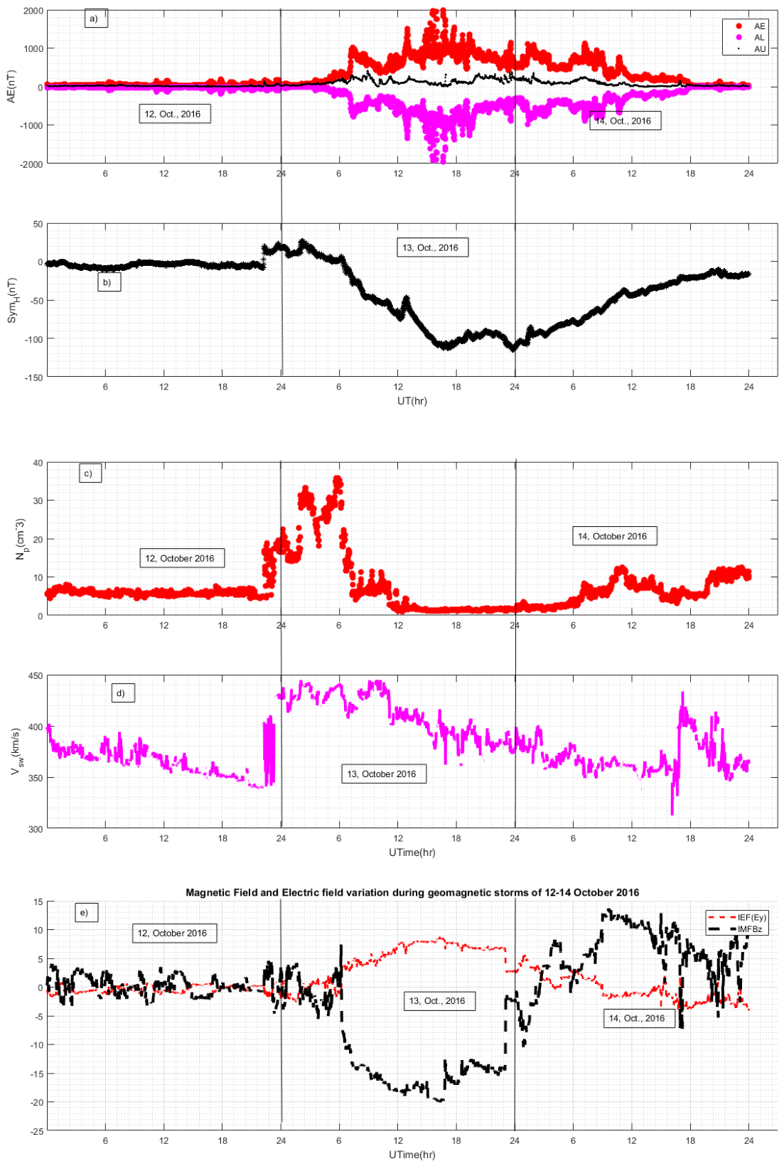
Figure 3.
Northern and Southern polar indeces of 12-14 , October 2016
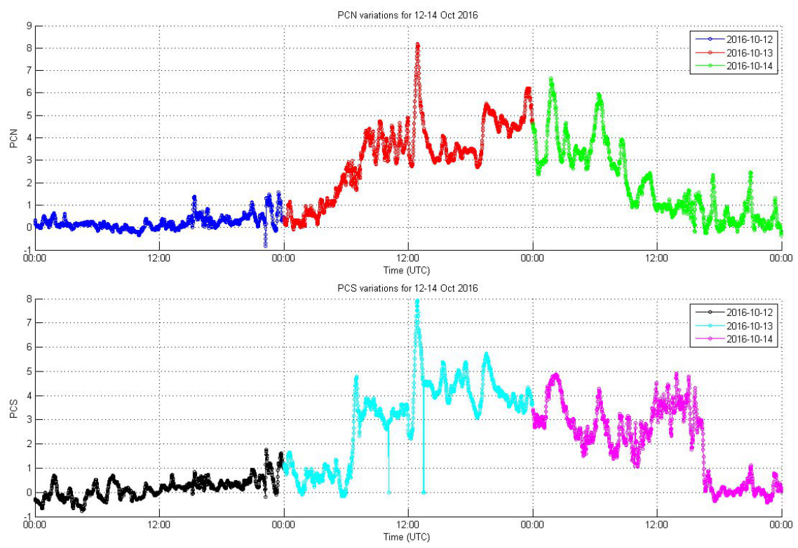
Figure 4.
Diurnal VTEC Variability of 12–14 October 2016 over the Northern Hemisphere
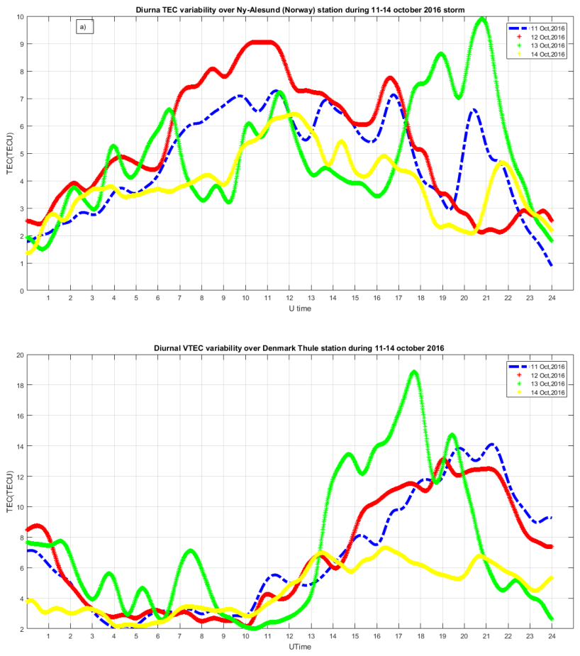

Table 1.
Selected GPS Stations with their codes and coordinates.
| S.No | ID | Locations | Geo.Lat | Geo. long | Geom.lat | LT(hr) |
|---|---|---|---|---|---|---|
| 1 | NYAL | Ny-Alesund,Norway | 78.82N | 11.86E | 78.4N | UT +1 |
| 2 | THU | Thule, Greenland | 76.57 N | -68.92E | 72.5N | UT-5 |
| 3 | PALM | Palmer Antartica | 64.7S | -64.05E | 61.23 S | UT-4 |
| 4 | SYOGO | East Ogleo Island | 69.0S | 39.58 E | 66.6S | UT+2:30 |
Disclaimer/Publisher’s Note: The statements, opinions and data contained in all publications are solely those of the individual author(s) and contributor(s) and not of MDPI and/or the editor(s). MDPI and/or the editor(s) disclaim responsibility for any injury to people or property resulting from any ideas, methods, instructions or products referred to in the content. |
© 2026 by the authors. Licensee MDPI, Basel, Switzerland. This article is an open access article distributed under the terms and conditions of the Creative Commons Attribution (CC BY) license (http://creativecommons.org/licenses/by/4.0/).
Copyright: This open access article is published under a Creative Commons CC BY 4.0 license, which permit the free download, distribution, and reuse, provided that the author and preprint are cited in any reuse.