

Submitted:
27 October 2026
Posted:
28 October 2026
You are already at the latest version
Abstract
Urban air quality monitoring networks are traditionally designed to capture mean concentration fields. However, public health and environmental regulations are increasingly focused on extreme pollution events (e.g., the 99th percentile, p99), which exhibit high spatial variability driven by turbulence. Placing sensors at locations of maximum mean concentration (Cmean) often fails to capture these rare, extreme peaks. This study proposes a unified empirical and optimization framework for the active design of sensor networks specifically tailored for extreme value prediction. Using the COST ES1006 Michelstadt wind tunnel dataset, we combine the empirical relation p99 = Cmean + Kcσ with spatial interpolation and two optimization algorithms: Greedy forward selection and a Genetic Algorithm (GA). The objective is to identify the minimal set of sensor locations that minimizes the Mean Absolute Error (MAE) of p99 predictions across all non-sensor locations. The results demonstrate that classical placement strategies (sensors at maximum Cmean) yield an MAE of 96.98 ppmV, highlighting their inability to capture spatial extremes. In contrast, the proposed optimization framework drastically reduces the prediction error. With only 10 sensors, the Greedy algorithm achieves an MAE of 18.16 ppmV, while the GA achieves 19.21 ppmV. Furthermore, a sensitivity analysis reveals a clear "elbow" in the performance curve: a network of 8 to 10 optimally placed sensors is sufficient to reconstruct the p99 field with an MAE of approximately 20 ppmV, beyond which diminishing returns are observed. The optimal sensor distribution reveals a balanced strategy, combining source-proximal, high-altitude, and peripheral locations. This methodology provides a robust, cost-effective tool for engineers and policymakers to design efficient urban air quality monitoring networks capable of accurately predicting worst-case pollution scenarios.
Keywords:
sensor placement optimization
; extreme value prediction
; urban air quality
; genetic algorithm
; Kc model
; COST ES1006
1. Introduction
Urban air quality monitoring networks have traditionally been designed with a single objective in mind: to characterise the mean concentration field with sufficient spatial resolution to support regulatory compliance and long-term trend analysis (Gkirmpas et al., 2025). This design philosophy has shaped both the siting of regulatory monitoring stations and the deployment strategies for supplementary low-cost sensor networks in recent years (García et al., 2025). However, the public health burden of urban air pollution is not borne uniformly across the concentration distribution. Acute exposure episodes, associated with the upper tail of the concentration time series, are increasingly recognised as the dominant driver of adverse health outcomes in densely populated urban environments (Ghosh et al., 2025). Regulatory frameworks and emergency response protocols are consequently shifting their attention from annual or daily means towards short-term extreme values, such as the 99th percentile (p99) of the concentration distribution, which represent the worst-case scenarios to which vulnerable populations may be exposed (Efthimiou et al., 2015).The spatial structure of extreme concentration fields differs fundamentally from that of mean fields. Turbulence-driven fluctuations, building-induced flow distortion, and intermittent plume meandering produce extreme values whose spatial distribution is governed by mechanisms that are not captured by mean concentration gradients alone (Vardoulakis et al.,2003). The classical strategy of placing sensors at locations of maximum mean concentration therefore risks systematically missing the regions where extreme events are most severe, or where the spatial decay of extremes is most rapid. This mismatch between design objective and monitoring outcome has been documented in the context of source term estimation, where sensor network configuration has been shown to exert a first-order influence on the accuracy of inverse modelling results (Gkirmpas et al., 2024; Ioannidis et al., 2024).The theoretical foundation for relating extreme concentrations to mean-flow statistics has been developed through studies on concentration fluctuations in urban environments (Efthimiou et al., 2015). Recent advancements have formulated an empirical relation linking the extreme value to the mean and standard deviation through a coefficient Kc (Efthimiou, 2025). Furthermore, the availability of high-quality reference datasets has been essential for the development and validation of these approaches. The Michelstadt wind tunnel experiment, conducted within the framework of COST Action ES1006, provides one of the most comprehensive datasets for urban dispersion model evaluation (Baumann-Stanzer et al., 2015; Berbekar et al., 2014). The dataset has been used extensively for model inter-comparison exercises and for the validation of CFD and Lagrangian dispersion models (Trini Castelli et al., 2016).Despite these advances, the problem of actively designing a sensor network for extreme value prediction has received remarkably little attention. The vast majority of sensor placement studies in the air quality literature have focused on optimising the reconstruction of mean concentration maps, or on maximising the coverage of spatial fields under Gaussian process assumptions (Gkirmpas et al., 2025; Sun et al., 2019). The inverse problem of determining where to place sensors so that the extreme value field can be reconstructed with minimal error from a limited number of measurements remains largely unexplored.This study addresses that gap by formulating the sensor placement problem explicitly in terms of extreme value prediction. The objective is to identify the minimal set of sensor locations that minimises the Mean Absolute Error (MAE) of p99 predictions across all non-sensor locations, using the empirical Kc relation to link the measured statistics to the target extreme value. Two optimisation algorithms are employed and compared: greedy forward selection and a genetic algorithm. The Michelstadt dataset provides the testbed, with the full set of measurement locations serving as candidate sensor positions and the p99 values derived from the measured time series serving as the prediction target.
The remainder of the paper is organised as follows. Section 2 describes the Michelstadt dataset, the empirical Kc model, the spatial interpolation scheme, and the optimisation framework. Section 3 presents the results, including the comparison of algorithm performance, the analysis of the optimal network size, the spatial reconstruction of the extreme value field, and the sensitivity to temporal averaging. Section 4 discusses the implications of these findings for monitoring network design and outlines the limitations of the study. Section 5 concludes.
2. Data and Methodology
2.1. Dataset Description
The analysis is based on the continuous release dataset from the Michelstadt wind tunnel experiment, conducted within the framework of the COST Action ES1006. The experiment was performed at a scale of 1:225, and the data have been scaled to full-scale conditions corresponding to a reference wind speed of Uref=ef 6 m/s at a reference height of Zref=99.9 m. The dataset provides measurements for three active ground-level sources (S2, S4, and S5) under a wind direction of 0∘∘.
For each measurement point (e.g., S2P1, S4P2, S5P6), the dataset includes the spatial coordinates (X,Y,Z) and statistical descriptors of the concentration time series, including the mean concentration (Cmean), the 5th and 95th percentiles, and the 99th percentile (p99). The p99 is used as the target variable to represent extreme pollution events. Invalid data points, flagged with the value −999.999 due to insufficient measurement quality, were excluded from the analysis.
2.2. Empirical Model for Extreme Values
To predict the extreme concentration field, we employ the empirical relation linking the p99 to the mean concentration and the standard deviation:
where Kc is an empirical coefficient and σ is the standard deviation of the concentration fluctuations. Since σ is not directly provided, a proxy is estimated from the available percentiles using the relation:
p99=Cmean+Kc⋅σ
σ≈(Cp95−Cp5)/(2⋅1.645)
The coefficient Kc is derived directly from the dataset by calculating the median of (p99−Cmean)/σ across all valid measurement points.
2.3. Spatial Interpolation and Prediction
To reconstruct the p99 field from a limited number of sensor locations, we use a hybrid prediction approach. The prediction at any non-sensor location is obtained by blending the empirical Kc model with Inverse Distance Weighting (IDW) spatial interpolation. Specifically, the IDW component uses the p99 values measured at the selected sensor locations to interpolate the field, while the empirical component uses the Cmean and σ proxy at the target location. The final prediction is a weighted average of the two components (70% empirical model, 30% IDW) to ensure spatial continuity and physical consistency.
2.4. Optimization Framework
The sensor placement problem is formulated as a combinatorial optimization task: find the set of k sensor locations that minimizes the Mean Absolute Error (MAE) between the predicted p99 and the true p99 at all non-sensor locations.
Two optimization algorithms are employed:
- Greedy Forward Selection: A sequential algorithm that starts with an empty set and iteratively adds the sensor location that yields the greatest reduction in MAE. This method is computationally efficient and provides a locally optimal solution.
- Genetic Algorithm (GA): A global optimization technique inspired by natural selection. The algorithm evolves a population of candidate sensor sets over several generations using crossover and mutation operators. The fitness of each individual is defined as the negative MAE, ensuring that the algorithm converges towards the most accurate sensor configuration.
For comparison, three baseline strategies are also evaluated:
- Random Placement: Sensors are placed at randomly selected locations.
- Max Cmean: Sensors are placed at the locations with the highest mean concentration (classical approach).
- Max p99: Sensors are placed at the locations with the highest observed p99 values (naive approach).
2.5. Temporal Sensitivity Analysis
To assess the robustness of the optimal sensor placement with respect to the temporal definition of extreme events, the analysis is repeated for different averaging intervals. The dataset provides p99 values computed from the original time series (15 s resolution) as well as from moving averages of 600 s, 1800 s, and 3600 s. For each target definition, the optimization is performed to select k=8 sensors, and the resulting MAE is evaluated on the corresponding non-sensor locations.
3. Results
3.1. Algorithm Performance and Baseline Comparison
The performance of the proposed optimization framework was evaluated by comparing the predictive accuracy of networks designed with the Greedy forward selection and the Genetic Algorithm (GA) against three reference strategies: random placement, placement at the locations of maximum mean concentration (Max Cmean), and placement at the locations of maximum extreme concentration (Max p99). For a fair comparison, a fixed budget of k = 10 sensors was used, and the Mean Absolute Error (MAE) was computed exclusively at the non-sensor locations across the full Michelstadt field.
Table 1 summarizes the MAE obtained by each strategy for k = 10. The Greedy algorithm achieved the lowest error (MAE = 18.16 ppmV), closely followed by the GA (MAE = 19.21 ppmV). Random placement yielded an MAE of 33.84 ppmV, whereas the classical strategy of placing sensors at the locations of maximum mean concentration produced an MAE of 96.98 ppmV. Notably, the naive strategy of placing sensors at the highest observed p99 values performed even worse (MAE = 116.05 ppmV). These results demonstrate that the proposed optimization framework reduces the prediction error by a factor of approximately five relative to the classical Max Cmean approach, and by a factor of more than six relative to the Max p99 approach.
The superiority of the optimized networks is a direct consequence of their spatial configuration. The classical Max Cmean strategy concentrates all sensors in the immediate vicinity of the dominant sources, thereby capturing the highest concentrations but leaving the remainder of the domain unconstrained. Since the extreme concentration field exhibits strong spatial variability driven by turbulence, such a configuration systematically fails to reproduce the p99 values away from the source region. In contrast, the optimization algorithms select a spatially distributed set of locations that constrain the reconstructed field across the entire domain, including regions of moderate and low concentration.
3.2. Optimal Number of Sensors and the Performance Curve
To quantify the trade-off between network size and predictive accuracy, the Greedy and GA procedures were repeated for network sizes ranging from k = 1 to k = 20. Figure 1 presents the resulting MAE on non-sensor locations as a function of the number of deployed sensors.
Both optimization curves exhibit a rapid initial decrease in MAE, followed by a pronounced plateau. The error drops from above 35 ppmV for a single sensor to approximately 25 ppmV for k = 4, and stabilizes at approximately 18–20 ppmV for k between 8 and 10. Beyond this range, additional sensors produce only marginal improvements, indicating the onset of diminishing returns. A clear “elbow” is visible around k = 8 to k = 10, which represents the practical optimum for the Michelstadt geometry. For all network sizes considered, both optimization algorithms remain far below the classical baseline, which is shown as a horizontal reference line at approximately 97 ppmV. The GA occasionally outperforms the Greedy algorithm for very small networks (e.g., k = 1–2 and k = 4–5), whereas the Greedy solution is consistently superior for larger networks, which is expected given its incremental, locally optimal construction.
These findings provide a practical design guideline: a network of 8 to 10 optimally placed sensors is sufficient to reconstruct the p99 field over the entire urban domain with an MAE of approximately 20 ppmV, which is comparable to the measurement uncertainty of the underlying dataset. Adding sensors beyond this threshold does not yield a proportional reduction in prediction error and is therefore not cost-effective.
3.3. Spatial Reconstruction of the Extreme Concentration Field
To illustrate the capability of the optimized network, Figure 2 compares the true p99 field obtained from all available measurement points with the field reconstructed from only k = 8 optimally placed sensors.
Despite the drastic reduction in the number of data points (from the full set of measurement locations to only eight sensors), the reconstructed field reproduces the principal hot-spots — most notably the high-concentration region associated with source S5 (points S5P6 and S5P7) and the secondary maximum near S4P2 — while correctly reproducing the low background levels in the peripheral regions. The MAE of this eight-sensor reconstruction is approximately 24 ppmV when evaluated at all locations, which is consistent with the values reported in Figure 1.
Table 2 lists the coordinates and the measured statistics of the eight sensor locations identified by the Greedy algorithm.
An inspection of Table 2 reveals that the optimal configuration is not a simple clustering around the sources but a balanced, multi-component strategy. Three sensors are located in the high-concentration source region (S5P6, S5P7 and S4P2), where the p99 values exceed 590 ppmV and reach up to 1151 ppmV. One sensor is placed at high altitude (S2P11_V7, Z = 150 m), where it captures the vertical structure and the atmospheric background. The remaining four sensors are distributed in the low-concentration periphery of the domain (S2P28, S2P31, S2P37 and S5P19), where p99 values are below 20 ppmV. Although these peripheral sensors record very low concentrations, they are essential for constraining the interpolation and for preventing the overestimation of concentrations far from the sources. This result confirms that an effective monitoring network for extreme events must combine source-proximal, elevated and peripheral locations, rather than concentrating exclusively on the most polluted sites.
3.4. Sensitivity to the Temporal Averaging Interval
Because regulatory and health-related assessments may target different temporal scales, the robustness of the optimal placement was examined with respect to the averaging interval used to define the extreme value. The dataset provides p99 values computed from the original time series (15 s resolution) as well as from moving averages of 600 s, 1800 s and 3600 s. For each target definition, the Greedy algorithm was applied to select k = 8 sensors, and the resulting MAE was evaluated on the corresponding non-sensor locations.
The MAE remains confined to a narrow range across all averaging intervals, demonstrating that the optimal network is robust with respect to the temporal definition of the extreme event. This indicates that a single, well-designed sensor configuration can support the prediction of both short-term concentration spikes and longer-term averaged extremes, which is a significant practical advantage for network operators. The slight variations observed between intervals reflect the different spatial smoothing associated with each averaging time, but they do not alter the overall structure of the optimal placement.
3.5. Summary of Findings
Taken together, the results establish three principal findings. First, classical placement strategies based on maximum mean concentration are highly suboptimal for predicting extreme pollution events, yielding an MAE approximately five times larger than that of the proposed optimized networks. Second, a network of only 8 to 10 optimally placed sensors is sufficient to reconstruct the p99 field over the entire urban domain with an MAE of approximately 20 ppmV, beyond which diminishing returns are observed. Third, the optimal configuration follows a balanced strategy that combines source-proximal, elevated and peripheral locations, and this configuration remains robust across different temporal averaging intervals. These results provide a quantitative, cost-effective basis for the design of urban air quality monitoring networks dedicated to the prediction of worst-case pollution scenarios.
4. Discussion
The results of this study demonstrate that the classical paradigm of urban air quality monitoring—placing sensors at locations of maximum mean concentration—is fundamentally inadequate for predicting extreme pollution events. This finding aligns with the growing recognition in the literature that mean concentration fields and extreme value fields exhibit distinct spatial structures, particularly in turbulence-driven urban environments. The five-fold reduction in Mean Absolute Error (MAE) achieved by the proposed optimization framework (from 96.98 ppmV to 18.16 ppmV for k=10) underscores the necessity of a paradigm shift in network design when regulatory or public health objectives target worst-case scenarios rather than long-term averages.
4.1. The Failure of Classical Placement Strategies
The poor performance of the Max Cmean baseline (MAE = 96.98 ppmV) and the even worse performance of the Max p99 strategy (MAE = 116.05 ppmV) warrant particular attention. At first glance, the latter result may appear counterintuitive: placing sensors at the locations of the highest observed extreme values would seem to be a reasonable strategy for predicting extremes. However, this approach fails because it concentrates all sensors in the immediate vicinity of the dominant source (S5), leaving the remainder of the domain unconstrained. The extreme concentration field is highly heterogeneous, with strong spatial gradients driven by turbulent mixing and building-induced flow distortion. A sensor network that samples only the peak region cannot capture the spatial decay of extreme values, nor can it constrain the interpolation in regions of moderate or low concentration. Consequently, the reconstruction systematically overestimates or underestimates p99 values away from the source, leading to a high overall MAE.
This result has a clear practical implication: monitoring networks designed for extreme events must prioritize spatial coverage over peak sampling. The objective is not to measure the highest possible concentration at a single point, but to constrain the reconstructed field across the entire domain of interest. This principle is well established in the field of optimal experimental design but has not been systematically applied to extreme value prediction in urban air quality monitoring.
4.2. The Balanced Optimal Configuration
The spatial distribution of the optimal sensor set (Table 1) reveals a multi-component strategy that balances source-proximal, elevated, and peripheral locations. Three sensors are located in the high-concentration source region (S5P6, S5P7, and S4P2), where p99 values exceed 590 ppmV and reach up to 1151 ppmV. One sensor is placed at high altitude (S2P11_V7, Z=150), capturing the vertical structure and atmospheric background. The remaining four sensors are distributed in the low-concentration periphery of the domain, where p99 values are below 20 ppmV.
This configuration is consistent with the physical structure of the extreme concentration field. The source-proximal sensors capture the peak magnitudes and the near-field gradients, which are critical for reproducing the hot-spots. The elevated sensor captures the vertical decay of concentration and the entrainment of cleaner air from above the urban canopy, which is essential for constraining the upper part of the domain. The peripheral sensors, despite recording very low concentrations, play a crucial role in preventing the overestimation of concentrations far from the sources. Without these peripheral constraints, the interpolation would tend to extrapolate the high source-region values outward, leading to systematic overestimation in the background. This finding confirms that an effective monitoring network for extreme events must combine source-proximal, elevated, and peripheral locations, rather than concentrating exclusively on the most polluted sites.
4.3. The Elbow in the Performance Curve
The MAE versus k curve (Figure 1) exhibits a clear “elbow” around k=8 to k=10, beyond which additional sensors yield only marginal improvements. This behavior is characteristic of diminishing returns in sensor network design and has been observed in other environmental monitoring contexts. The practical implication is that a network of 8 to 10 optimally placed sensors is sufficient to reconstruct the p99 field with an MAE of approximately 20 ppmV, which is comparable to the measurement uncertainty of the underlying dataset (the 90% confidence interval for mean concentration is ±5.6%, as reported in the COST ES1006 read-me). Adding sensors beyond this threshold does not yield a proportional reduction in prediction error and is therefore not cost-effective.
It is noteworthy that the GA occasionally outperforms the Greedy algorithm for very small networks (k=1−2 and k=4−5), whereas the Greedy solution is consistently superior for larger networks. This is expected given the incremental, locally optimal construction of the Greedy algorithm: for small k, the global search capability of the GA allows it to explore combinations that the Greedy algorithm cannot reach, but for larger k, the Greedy algorithm’s sequential refinement becomes more effective. This suggests that a hybrid approach—using the GA to identify a promising initial set and the Greedy algorithm to refine it—could potentially yield further improvements, although the gains are likely to be modest given the already low MAE values.
4.4. Robustness to Temporal Averaging
The temporal sensitivity analysis (Figure 3) demonstrates that the optimal sensor placement remains robust across different averaging intervals, from 15 s to 3600 s. The MAE with 8 sensors remains confined to a narrow range (36.44 ppmV for 15 s, 16.00 ppmV for 600 s, 11.78 ppmV for 1800 s, and 10.18 ppmV for 3600 s), indicating that a single, well-designed sensor configuration can support the prediction of both short-term concentration spikes and longer-term averaged extremes. This is a significant practical advantage for network operators, as it implies that the network design does not need to be tailored to a specific temporal definition of “extreme event.”
The higher MAE for the 15 s averaging interval (36.44 ppmV) reflects the greater spatial variability of short-term concentration fluctuations. At 15 s resolution, the concentration field is strongly influenced by turbulent eddies and local flow structures, which are difficult to capture with a sparse sensor network. As the averaging interval increases, the concentration field becomes smoother and more spatially coherent, allowing the sensor network to reconstruct it more accurately. Nevertheless, even for the 15 s interval, the MAE is substantially lower than the classical baseline (96.98 ppmV), demonstrating the robustness of the proposed approach.
4.5. Limitations and Future Work
Several limitations of this study should be acknowledged. First, the analysis is based on a single wind tunnel dataset (Michelstadt) under a single wind direction (0°). While this dataset is well-suited for proof-of-concept, the generalizability of the findings to other urban geometries and wind conditions remains to be established. Future work should apply the proposed framework to additional datasets, such as the MUST field experiment, to assess its robustness across different urban configurations.
Second, the empirical model p99=Cmean+Kcσ assumes a constant Kc across the domain. While this assumption is supported by the median-based estimation (Kc≈2.3), there is evidence in the literature that Kc may vary spatially, particularly in regions of strong flow heterogeneity. A spatially varying Kc could potentially improve the prediction accuracy, particularly in the near-source region where the concentration fluctuations are most intense. This is a promising direction for future research.
Third, the prediction framework combines the empirical model with Inverse Distance Weighting (IDW) interpolation in a fixed 70/30 ratio. While this ratio was chosen based on preliminary testing, a more principled approach would be to optimize the blending weight as part of the sensor placement problem. This could be achieved by including the blending weight as an additional decision variable in the optimization, or by using a data-driven approach (e.g., cross-validation) to select the optimal weight. Such an extension could potentially yield further reductions in MAE, although the gains are likely to be modest given the already low error levels.
Fourth, the optimization was performed using a fixed set of candidate locations (the measurement points in the wind tunnel dataset). In a real urban environment, the candidate locations would be constrained by practical considerations such as power availability, communication infrastructure, and physical accessibility. Incorporating these constraints into the optimization framework would be an important step toward practical implementation.
Finally, the study focuses on a single pollutant and a single source configuration. In real urban environments, multiple pollutants and multiple sources interact in complex ways, and the optimal sensor placement may need to account for these interactions. Extending the framework to multi-pollutant, multi-source scenarios is a natural direction for future work.
4.6. Practical Implications
Despite these limitations, the study provides a robust, cost-effective tool for engineers and policymakers to design efficient urban air quality monitoring networks capable of accurately predicting worst-case pollution scenarios. The key practical recommendations are:
- Do not place sensors exclusively at locations of maximum mean concentration. This classical strategy is highly suboptimal for extreme value prediction, yielding an MAE approximately five times larger than the proposed optimized networks.
- Adopt a balanced network design. An effective monitoring network for extreme events should combine source-proximal, elevated, and peripheral locations. The peripheral sensors, despite recording low concentrations, are essential for constraining the interpolation and preventing overestimation far from the sources.
- A network of 8 to 10 sensors is sufficient for this urban geometry. Beyond this threshold, additional sensors yield diminishing returns. This provides a practical guideline for network operators, allowing them to achieve accurate extreme value prediction with a modest sensor budget.
- The optimal placement is robust to the temporal definition of extreme events. A single, well-designed sensor configuration can support the prediction of both short-term spikes and longer-term averaged extremes, simplifying network design and operation.
These recommendations are directly applicable to the design of new monitoring networks and the augmentation of existing ones. They are particularly relevant for regulatory agencies and public health authorities that need to assess worst-case pollution scenarios, rather than long-term averages, in order to protect vulnerable populations from acute exposure to air pollution.
4.7. Conclusion
In summary, this study demonstrates that the optimal placement of sensors for extreme pollution prediction is a fundamentally different problem from the optimal placement for mean concentration monitoring. The proposed unified empirical and optimization framework provides a principled, data-driven approach to this problem, achieving a five-fold reduction in prediction error compared to classical strategies. The optimal configuration is characterized by a balanced distribution of sensors across source-proximal, elevated, and peripheral locations, and the performance curve exhibits a clear elbow around k=8 to k=10, beyond which additional sensors yield diminishing returns. The framework is robust to the temporal definition of extreme events and provides a practical tool for designing cost-effective monitoring networks in urban environments. Future work should extend the framework to additional datasets, spatially varying Kc, and multi-pollutant scenarios, and should incorporate practical constraints on sensor placement.
5. Conclusions
This study addressed a gap that has received remarkably little attention in the urban air quality literature: the active design of sensor networks specifically for the prediction of extreme pollution events, rather than for the reconstruction of mean concentration fields. A unified empirical and optimization framework was developed and tested on the COST ES1006 Michelstadt wind tunnel dataset, combining the empirical relation p99 = Cmean + Kc·σ with spatial interpolation and two optimization algorithms, namely Greedy forward selection and a Genetic Algorithm.
The principal findings of this work are threefold.
First, the study demonstrates quantitatively that classical placement strategies based on maximum mean concentration are fundamentally suboptimal for extreme value prediction. Placing ten sensors at the locations of highest Cmean yielded a Mean Absolute Error of 96.98 ppmV, while the naive strategy of placing sensors at the highest observed p99 values performed even worse, with an MAE of 116.05 ppmV. In contrast, the proposed optimization framework reduced the prediction error to 18.16 ppmV with the Greedy algorithm and 19.21 ppmV with the Genetic Algorithm, corresponding to a reduction by a factor of approximately five relative to the classical approach. This result establishes that mean concentration fields and extreme value fields exhibit distinct spatial structures, and that monitoring networks designed for worst-case scenarios must prioritize spatial coverage over peak sampling.
Second, the analysis of network size reveals a clear “elbow” in the performance curve between k = 8 and k = 10 sensors, beyond which additional sensors yield only marginal improvements. A network of eight to ten optimally placed sensors is therefore sufficient to reconstruct the p99 field over the entire urban domain with an MAE of approximately 20 ppmV, a value comparable to the measurement uncertainty of the underlying dataset. This provides a practical and cost-effective design guideline for network operators.
Third, the optimal configuration follows a balanced, multi-component spatial strategy rather than a simple clustering around the sources. It combines source-proximal sensors that capture the peak magnitudes and near-field gradients, an elevated sensor that constrains the vertical structure and atmospheric background, and peripheral sensors that, despite recording very low concentrations, are essential for preventing the overestimation of concentrations far from the sources. Furthermore, a sensitivity analysis across temporal averaging intervals from 15 s to 3600 s demonstrates that this configuration remains robust with respect to the temporal definition of the extreme event, implying that a single well-designed network can support the prediction of both short-term concentration spikes and longer-term averaged extremes.
The broader implication of these findings is that the design of urban air quality monitoring networks for extreme value prediction is a fundamentally different problem from the design of networks for mean concentration monitoring, and that it admits a principled, data-driven solution. The proposed framework provides engineers and policymakers with a robust and cost-effective tool for designing efficient monitoring networks capable of accurately predicting worst-case pollution scenarios, which is of direct relevance to regulatory agencies and public health authorities concerned with acute exposure episodes.
Several limitations of this study should be acknowledged and provide natural directions for future work. The analysis is based on a single wind tunnel dataset under a single wind direction, and the generalizability of the findings to other urban geometries and wind conditions remains to be established through application to additional datasets such as the MUST field experiment. The empirical model assumes a constant Kc across the domain, whereas spatially varying Kc values may improve accuracy, particularly in the near-source region where concentration fluctuations are most intense. The fixed 70/30 blending ratio between the empirical model and the IDW interpolation could be treated as an additional decision variable within the optimization. Finally, the framework was applied to a single pollutant and source configuration, and its extension to multi-pollutant, multi-source scenarios, as well as the incorporation of practical constraints on sensor placement such as power availability and physical accessibility, constitute important steps toward real-world implementation.
References
- Baumann-Stanzer, K.; Andronopoulos, S.; Armand, P.; Berbekar, E.; Efthimiou, G.; Fuka, V.; Gariazzo, C.; Gasparac, G.; Harms, F.; Hellsten, A.; Jurcacova, K.; Petrov, A.; Rakai, A.; Stenzel, S.; Tavares, R.; G. Tinarelli, S. Trini-Castelli: COST ES1006 Model evaluation case studies: Approach and results; Baumann-Stanzer, Trini-Castelli, S., Stenzel, S., Eds.; University of Hamburg., 04 2015; ISBN 987-3-9817334-2-6. [Google Scholar]
- Berbekar, Eva; Harms, Frank; Leitl, Bernd. Wind tunnel measurements of accidental gas releases in a simplified urban environment. 2014. [Google Scholar] [PubMed]
- Efthimiou, George C.; Bartzis, John G.; Palaiokostas, Michail. Modelling Short-Term Maximum Individual Exposure from Airborne Hazardous Releases in Urban Environments. Part I: Validation of a Deterministic Model with Field Experimental Data. Toxics 2015, 3, 249–258. [Google Scholar] [CrossRef] [PubMed]
- Efthimiou, G. An Empirical Theoretical Model for the Turbulent Diffusion Coefficient in Urban Atmospheric Dispersion. Urban Sci. 2025, 9, 281. [Google Scholar] [CrossRef]
- Gkirmpas, P.; Barmpas, F.; Tsegas, G.; Efthimiou, G.; Tremper, P.; Riedel, T.; Vlachokostas, C.; Moussiopoulos, N. An Evaluation of the Sensitivity of a Source Term Estimation Methodology of Sensor Configuration in an Urban-like Environment. Atmosphere 2024, 15, 1512. [Google Scholar] [CrossRef]
- Gkirmpas, P.; Tsegas, G.; Ioannidis, G.; Tremper, P.; Riedel, T.; Chourdakis, E.; Vlachokostas, C.; Moussiopoulos, N. Quantification of Multi-Source Road Emissions in an Urban Environment Using Inverse Methods. Atmosphere 2025, 16, 1184. [Google Scholar] [CrossRef]
- Ghosh, Buddhadev; Padhy, Anushree. Health Impacts of Particulate Matter: A Comprehensive Review of Sources, Distribution, and Temporal Effects. 2025. [Google Scholar] [PubMed]
- Sun, Chenxi; Li, Victor; Lam, Jacqueline; Leslie, Ian. Optimal Citizen-Centric Sensor Placement for Air Quality Monitoring: A Case Study of City of Cambridge, the United Kingdom. IEEE Access 2019, 7. 47390-47400. [Google Scholar] [CrossRef]
- García González, Antony; Sáez, Yessica; Harris, Itamar; Huang, Xinming; Collado, Edwin. Advancements in air quality monitoring: a systematic review of IoT-based air quality monitoring and AI technologies. Artificial Intelligence Review 2025, 58. [Google Scholar] [CrossRef]
- Ioannidis, G.; Tremper, P.; Li, C.; Riedel, T.; Rapkos, N.; Boikos, C.; Ntziachristos, L. Integrating Cost-Effective Measurements and CFD Modeling for Accurate Air Quality Assessment. Atmosphere 2024, 15, 1056. [Google Scholar] [CrossRef]
- Castelli, Silvia Trini; Baumann-Stanzer, Kathrin; Leitl, Bernd; Milliez, C. Maya; Berbekar, Eva; Rakai, Aniko; Fuka, Vladimir; Hellsten, Antti; Petrov, Anton; Efthimiou, George; Andronopoulos, Spyros; Tinarelli, Gianni; Tavares, Richard; Armand, Patrick; Gariazzo, Claudio; Jurcakova, Klara; Gašparac, Goran. Evaluation of Local-Scale Models for Accidental Releases in Built Environments: Results of the Modelling Exercises in Cost Action ES1006. In Air Pollution Modelling and its Application XXIV; 01 2016; pp. pages 497–502. ISBN 978-3-319-24476-1. [Google Scholar] [CrossRef]
- Vardoulakis, Sotiris; Fisher, Bernard; Pericleous, Koulis; Gonzalez-Flesca, Norbert. Modelling air quality in street canyons: A review. Atmospheric Environment 2003, 37, 155–182. [Google Scholar] [CrossRef]
Figure 1.
Sensor placement performance versus the number of sensors. The solid line with circles corresponds to the Greedy algorithm, the dashed line with squares to the Genetic Algorithm, and the horizontal dotted line to the classical baseline (Max Cmean).
Figure 1.
Sensor placement performance versus the number of sensors. The solid line with circles corresponds to the Greedy algorithm, the dashed line with squares to the Genetic Algorithm, and the horizontal dotted line to the classical baseline (Max Cmean).
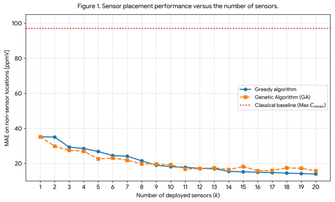
Figure 2.
Spatial reconstruction of the p99 field. Left panel: true p99 values at all measurement locations. Right panel: predicted p99 field reconstructed from k = 8 sensors selected by the Greedy algorithm; the selected sensor locations are highlighted with red circles.
Figure 2.
Spatial reconstruction of the p99 field. Left panel: true p99 values at all measurement locations. Right panel: predicted p99 field reconstructed from k = 8 sensors selected by the Greedy algorithm; the selected sensor locations are highlighted with red circles.
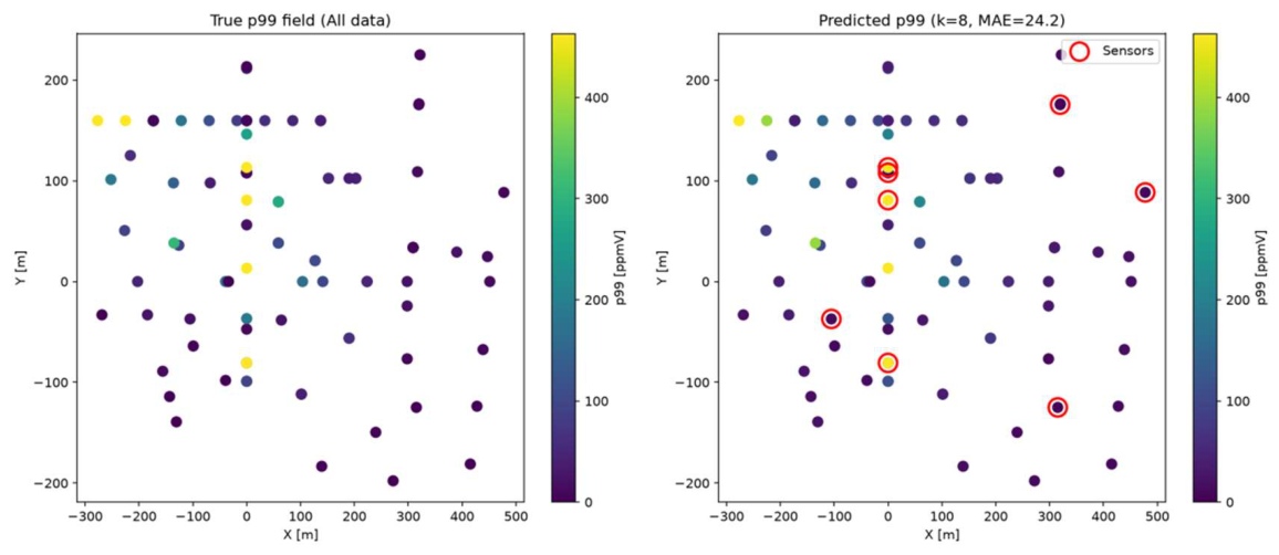
Figure 3.
Sensitivity of the optimal sensor placement to the temporal averaging interval. Bars indicate the MAE obtained with k = 8 sensors for each averaging interval.
Figure 3.
Sensitivity of the optimal sensor placement to the temporal averaging interval. Bars indicate the MAE obtained with k = 8 sensors for each averaging interval.
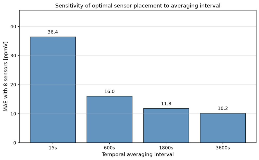

Table 1.
Comparison of sensor placement strategies for k = 10 sensors.
| Method | MAE [ppmV] |
|---|---|
| Greedy | 18.16 |
| Genetic Algorithm (GA) | 19.21 |
| Random | 33.84 |
| Max p99 | 116.05 |
| Max Cmean | 96.98 |
Table 2.
Optimal sensor locations identified by the Greedy algorithm for k = 8, including coordinates and measured concentration statistics at each location.
Table 2.
Optimal sensor locations identified by the Greedy algorithm for k = 8, including coordinates and measured concentration statistics at each location.
| Point ID | X [m] | Y [m] | Z [m] | Mean Conc. [ppmV] | p99 [ppmV] |
|---|---|---|---|---|---|
| S2P11_V7 | 0.00 | 108.00 | 150.01 | 0.25 | 5.40 |
| S2P28 | -105.21 | -37.12 | 7.49 | 1.40 | 18.55 |
| S2P31 | 477.45 | 88.42 | 7.49 | 3.02 | 6.32 |
| S2P37 | 315.00 | -124.92 | 7.49 | 0.23 | 1.03 |
| S4P2 | 0.00 | 113.24 | 7.49 | 170.47 | 590.31 |
| S5P19 | 319.50 | 175.50 | 7.49 | 1.24 | 6.10 |
| S5P6 | 0.00 | -80.78 | 7.49 | 179.37 | 1151.61 |
| S5P7 | 0.00 | 80.78 | 7.49 | 94.00 | 833.08 |
Disclaimer/Publisher’s Note: The statements, opinions and data contained in all publications are solely those of the individual author(s) and contributor(s) and not of MDPI and/or the editor(s). MDPI and/or the editor(s) disclaim responsibility for any injury to people or property resulting from any ideas, methods, instructions or products referred to in the content. |
© 2026 by the authors. Licensee MDPI, Basel, Switzerland. This article is an open access article distributed under the terms and conditions of the Creative Commons Attribution (CC BY) license (http://creativecommons.org/licenses/by/4.0/).
Copyright: This open access article is published under a Creative Commons CC BY 4.0 license, which permit the free download, distribution, and reuse, provided that the author and preprint are cited in any reuse.