

Submitted:
25 October 2026
Posted:
27 October 2026
You are already at the latest version
Abstract
Predicting the unobserved rear half of an acceleration time-history curve can make automotive safety evaluation more efficient. This study compares two deep-learning models, LSTM+CNN and TCN+GAN, for reconstructing post-impact acceleration signals from their observed front halves. The workflow includes signal preprocessing, statistical feature augmentation, and model training with reconstruction losses; TCN+GAN also uses an adversarial loss. We assess pointwise accuracy, temporal alignment, and physical consistency, and examine how the predictions affect downstream Head Injury Criterion (HIC) estimates. In the reported tests, TCN+GAN preserved key dynamic features more closely and produced more physically plausible signals than LSTM+CNN. The results suggest that it could serve as a surrogate in some simulation tasks and support injury prediction.
Keywords:
time-history prediction
; automotive crash acceleration
; TCN+GAN
; LSTM+CNN
; Head Injury Criterion (HIC)
1. Introduction
Time-history curves are essential data structures that characterize the evolution of physical, physiological, or abstract quantities over time. They form the analytical backbone of dynamic system studies across a wide range of scientific and industrial domains. In structural engineering, time-history curves are used to capture ground motion and structural vibrations during seismic events [1], enabling precise dynamic response analysis. In automotive safety engineering, they represent acceleration, velocity, and force responses during crash tests, serving as the foundation for injury prediction metrics such as the Head Injury Criterion (HIC) [2]. In aerospace systems, time-history signals are employed to monitor vehicle attitude, engine dynamics, and pressure fluctuations [3]. In biomedical research, they depict continuous physiological signals like heart rate, brain activity, and blood oxygen levels [4]. Even in finance and meteorology, time-dependent data are visualized as curves to analyze volatility or forecast weather patterns [5,6]. Across these diverse fields, the ability to predict the rear half of a time-history curve, i.e., to forecast future signal behavior from the observed front portion, is not merely a test of modeling capability, but a matter of practical importance. Accurate rear-half prediction can drastically reduce simulation time, enable real-time decision-making, prevent cascading system failures, and reduce dependency on costly physical experiments by providing high-fidelity synthetic alternatives.
Historically, the prediction of time-history data has relied on classical time series models, such as autoregressive (AR), moving average (MA), and their combinations (ARMA/ARIMA) [7,8], which operate under the assumptions of stationary signal behavior and linear system dynamics. These methods are analytically tractable and computationally efficient, but their applicability is limited in domains characterized by strong nonlinearities, abrupt transitions, or long-term dependencies. Kalman filters and wavelet-based decomposition techniques have also been used to forecast future signals with some success, particularly in the control and signal compression fields [9]. However, these models often underperform when confronted with noisy or high-dimensional data, where manually engineered features fail to capture the inherent complexity of the underlying processes. The advent of machine learning has introduced data-driven approaches to time series forecasting, where models learn temporal patterns directly from the raw, unprocessed data. Recurrent Neural Networks (RNNs), particularly Long short Term Memory (LSTM) networks, have demonstrated strong capability in modeling sequences with temporal dependencies, achieving notable success in domains such as speech synthesis [10] and physiological signal modeling. Temporal Convolutional Networks (TCNs), as an alternative architecture, employ dilated convolutions to efficiently capture long-range dependencies while enabling parallel processing, thereby mitigating several limitations of RNNs. Generative Adversarial Networks (GANs), originally developed for image generation [11], have been extended to the temporal domain to produce or complete time series with improved realism. Despite their considerable capabilities, these methods encounter specific challenges when applied in isolation: RNNs may suffer from vanishing gradient issues, GANs can be unstable to train, and TCNs may offer limited fine-grained interpretability. Therefore, integrating these complementary techniques presents a compelling strategy for predicting complex, multi-scale signals.
Recent literature and empirical studies increasingly demonstrate the effectiveness of combining multiple AI paradigms particularly TCNs and GANs—for modeling structured, nonlinear time series across diverse. For instance, in healthcare, GAN-based models have been used to generate missing sections in electrocardiogram (ECG) and functional near-infrared spectroscopy (fNIRS) data with high fidelity [12], enabling improved diagnosis under incomplete monitoring. In traffic prediction, TCN-GAN hybrids have been used to extrapolate vehicle trajectories and passenger flows with spatiotemporal consistency [13]. In the context of smart manufacturing, predictive models combining convolutional and generative elements have shown success in anticipating equipment faults before they materialize [14]. Drawing on this growing body of work, we hypothesize that applying a similar integrated strategy to the prediction of crash acceleration curves particularly the rear half, which contains complex but structured post-impact dynamics will lead to accurate and realistic signal reconstruction. As evidenced in our previously disclosed patents, crash acceleration curves exhibit both deterministic patterns (e.g., vehicle deformation phases) and stochastic fluctuations (e.g., secondary impacts or structural resonance). The hybrid TCN-LSTM-GAN model is designed to simultaneously capture these multi-scale, nonlinear behaviors through a modular structure: TCN for long-range dependencies, LSTM for sequential integrity, and GAN for adversarial refinement of realism. This integrated architecture aligns well with the physical characteristics of automotive crash data and the demands of HIC-based safety evaluations.
In this paper, we present a deep learning-based approach to the problem of rear-half prediction in time-history curves. Our method leverages a hybrid neural network architecture that combines LSTM modules for long-term sequence modeling, CNN/TCN components for capturing localized temporal features, and a generative adversarial learning mechanism for producing plausible and high-fidelity signal completions. We evaluate the model using automotive crash acceleration datasets, which are critical in vehicle safety certification and simulation processes [15]. By feeding only the front half of the acceleration curve into our model, we predict the rear half and subsequently compute derived metrics such as HIC to assess prediction utility. Quantitative results demonstrate that the model achieves high accuracy (R2 > 0.97) and realistic signal morphology, with predicted HIC values showing less than 3% deviation from ground truth. Beyond performance metrics, our results suggest a significant reduction in simulation and test cycle time, highlighting the method’s practical value. This work makes the following contributions: (1) we propose and validate a novel hybrid model for rear-half prediction of time-history curves, (2) we demonstrate its effectiveness on a real-world, high-impact application in automotive safety engineering, and (3) we position this technique as a generalizable solution for accelerating time-dependent simulation workflows in other domains.
2. Method
2.1. Mathematical Characteristics of Time-History Curves
Definition and Formulation:
Let denote a time-history curve that represents a dynamic physical variable—such as acceleration, stress, or pressure—measured over a time domain [0,T]. Formally, the curve is discretized as a time series:
This discrete time-history curve inherently satisfies strong temporal autocorrelation, typically quantified by an autocorrelation function (ACF):
where , and is the lag.
Information Embedded in Time-History Curves:
Each time-history curve encapsulates a wealth of information about the underlying physical system, including:
- 1)
- Initial conditions: implicitly encoded in the first few time steps.
- 2)
- Structural properties: revealed through frequency and damping patterns.
- 3)
- External excitations or boundary loads: apparent from shock, impulse, or sustained forcing profiles.
A critical hypothesis in this paper is that the front half of a well-formed time-history curve {a1,…,aT/2} contains sufficient latent features to infer or reconstruct the rear half {aT/2+1,…,aT}. Let us define:
The task is to learn a function , parameterized by , that minimizes:
subject to constraints on smoothness, continuity, and physical plausibility (e.g., conservation laws, monotonicity).
This framing positions the rear-half prediction as a functional approximation problem using the front half as an observable proxy for the full system dynamics.
2.2. Model Structures and Theoretical Principles
2.2.1. LSTM + CNN Hybrid Model
The LSTM+CNN hybrid model is designed to address the dual challenge inherent in time-history signal prediction: the need to capture long-range temporal dependencies as well as localized high-frequency phenomena. In time-history curves such as those observed in automotive crash acceleration data, key structural information is distributed globally across time (e.g., deformation behavior, impact sequence), while crucial metrics like HIC are sensitive to short bursts or peaks in acceleration (e.g., within 10–50 ms windows). Hence, a model must simultaneously learn the slow-varying global dynamics and transient high-magnitude changes.
Let the input front-half signal be denoted as , where xt is the measured acceleration at time step t. We define the LSTM encoder as a nonlinear operator , such that:
The final hidden state serves as a compressed temporal summary encoding of the front half.
Concurrently, a CNN module operates on sliding windows of the input to extract localized temporal patterns, defined by:
where * denotes 1D convolution, f is the number of filters, and is an activation function (typically ReLU).
These CNN feature maps z = {zk+1,…,zT/2−k} are passed through a max-pooling operation to preserve dominant transient features.
The fusion mechanism integrates the outputs from LSTM and CNN using a concatenation and linear transformation:
where [⋅;⋅] denotes vector concatenation and Wf projects the fused features to a common embedding dimension.
The rear half prediction is then obtained via a fully connected regression decoder:
Design Rationale and Advantages:
- 1)
- The LSTM encoder captures slow-varying, long-range dependencies, such as energy transfer and structural phase evolution in crash dynamics.
- 2)
- The CNN module identifies high-magnitude peaks and derivatives relevant to HIC, which is defined over short-time integral windows of squared acceleration.
- 3)
- The fusion strategy allows the model to incorporate both global and local views of the signal, enhancing accuracy and robustness.
- 4)
- Training with MSE loss ensures stable convergence, while dropout regularization in both paths prevents overfitting [16].
2.2.2. TCN + GAN Model
The Temporal Convolutional Network (TCN) combined with a Generative Adversarial Network (GAN) forms a robust hybrid model tailored for the long-range and distribution-preserving prediction of time-history curves [17]. This architecture addresses limitations present in recurrent models by allowing fixed-latency inference and enabling parallel training, while GANs mitigate the deterministic bias of standard regression losses and enforce output realism.
- TCN Structure and Mathematical Formulation:
Let the front half of the time-history sequence be x = {x1,x2,…,xT/2}. A TCN processes this input using dilated, causal convolutions. A 1D dilated convolution with dilation factor d and kernel size k is defined as:
Here, causality ensures that the output at time t does not depend on future inputs x>t, while dilation allows the receptive field to grow exponentially with depth. For a network with L layers and doubling dilation d = 2l, the total receptive field R is:
Such design allows a TCN to model dependencies spanning hundreds of time steps, a desirable property for capturing extended crash sequences.
- 2.
- GAN Integration and Adversarial Loss:
The TCN output predicts the rear half
of the curve. To enhance realism, a discriminator D is trained to distinguish
between true and generated sequences. The objective follows the conditional GAN
framework:
Here, G is the TCN-based generator and D is a CNN-based binary classifier. Both models are optimized iteratively using adversarial training strategies.
- 3.
- Combined Loss Function
To preserve numerical fidelity and enforce signal realism, the generator loss combines adversarial and reconstruction terms:
where . The weighting
parameters balance precision and
realism.
- 4.
- Design Advantages and Application to HIC Prediction
- 1)
- TCN's large receptive field captures extended dynamic phases, such as crumple initiation and rebound oscillations during automotive crashes.
- 2)
- Causal structure ensures predictions are physically consistent with real-time operation, i.e., no leakage from future data.
- 3)
- GAN discriminators penalize unrealistic patterns, such as overly smooth or noisy predictions that do not match empirical signal distributions.
- 4)
- The hybrid loss improves both pointwise accuracy and high-level statistical properties, crucial for safety metrics like HIC which depend on power-weighted integrals of acceleration.
Empirical results (detailed in Section 4) confirm that TCN+GAN models more effectively capture multimodal variability compared to pure regression models.
2.2.3. Comparative Analysis of LSTM+CNN and TCN+GAN Approaches
LSTM+CNN and TCN+GAN take different approaches to predicting the rear half of a time-history curve. LSTM+CNN combines recurrent sequence modeling with convolutional feature extraction, whereas TCN+GAN uses temporal convolutions and adversarial training to generate a realistic signal. Both models use past dynamics to predict the unobserved segment, but differ in their design, training behavior, interpretability, and generalization. LSTM+CNN performs well when the target signal follows a relatively consistent structure, such as clearly defined collision phases. Its recurrent layers capture longer-term dependencies, while the CNN responds to short transients. This combination can be useful for measures such as HIC, which are sensitive to brief, high-magnitude events. Its performance, however, can depend on sequence length and the characteristics of the input data.
TCN+GAN uses a fixed-depth temporal convolutional network with dilation, allowing its receptive field to expand while keeping training computationally efficient. The GAN component encourages generated signals to match the data distribution, which can help when crash responses are multimodal or non-Gaussian. GAN training can also be unstable: the generator and discriminator need to remain balanced, and a discriminator that overfits may reject valid but less common predictions.
LSTM+CNN is a practical choice when predictions need to be relatively deterministic and the contribution of sequential and local features must be interpreted. TCN+GAN is better suited to generative tasks where matching the statistical properties of observed signals matters, including surrogate modeling and data completion in safety-critical applications.
2.3. Practical Implementation of AI Architectures
2.3.1. Feature Extraction and Preprocessing
Feature extraction from the front half of the time-history curve xf = [x0,x1,…,xN/2−1] is critical to maximize the representational capacity of the predictive models. ince raw signals are often contaminated with noise, preprocessing and domain-specific transformations are applied as a standardized pipeline.
First, Z-score normalization is performed to scale each signal, ensuring zero mean and unit variance. Each signal is normalized such that:
This is followed by smoothing operations, such as moving average or Gaussian filtering, to suppress high-frequency noise, and linear detrending to remove global bias or gradual system drift. When higher-order dynamics are relevant, differential features such as velocity and acceleration are computed from the normalized curve. This is followed by smoothing operations, such as moving average or Gaussian filtering, to suppress high-frequency noise, and linear detrending to remove global bias or gradual system drift. When higher-order dynamics are relevant, differential features such as velocity and acceleration are computed from the normalized curve.
In addition to these preprocessing steps, several statistical features are extracted to enrich the model’s input space. These include the peak value max(xi) and its corresponding time index argmax(xi), short-time energy (STE, i.e.,, root mean square (RMS, i.e.,) amplitude, and the zero-crossing rate (ZCR) representing the frequency of sign changes in the signal. Furthermore, spectral entropy is calculated over the FFT spectrum to quantify the distribution and spread of frequency components.
These statistical descriptors may be appended as auxiliary model inputs or employed for data stratification during training, thereby enhancing the model’s ability to capture both temporal and frequency-domain characteristics of the input sequence.
2.3.2. Network Architecture and Parameterization
The LSTM+CNN architecture is designed with two main processing branches. The LSTM branch comprises two stacked layers, each containing 128 hidden units, producing a final hidden state vector that encodes the long-term temporal dependencies of the input sequence. In parallel, the CNN branch processes the signal through three sequential one-dimensional convolutional layers with kernel sizes of [3,5,7], respectively, each equipped with 64 filters and followed by a ReLU activation and max pooling. The resulting feature maps are flattened to form a compact representation of localized temporal features. Outputs from the LSTM and CNN branches are then concatenated in a fusion layer, which is passed through a dense layer of 256 neurons with ReLU activation before reaching the final regression module, a fully connected multilayer perceptron (MLP) with a linear activation function.
The TCN+GAN architecture follows a different design paradigm. Its generator is a Temporal Convolutional Network (TCN) composed of 5 layers with exponentially increasing dilation factors d = 1,2,4,8,16, each using a kernel size of 3. Residual connections and layer normalization are applied between layers to improve stability and gradient flow. The generator produces the predicted signal output . The discriminator, implemented as a one-dimensional CNN, consists of three layers with kernel sizes [5, 3, 3] and a stride of 1. Each convolutional layer is followed by a LeakyReLU activation with , and the final layer is a dense layer with a sigmoid activation function, yielding a probability score that distinguishes real from generated sequences.
2.3.3. Training Configuration and Loss Optimization
Let denote the model prediction.
For the LSTM+CNN architecture, the training objective is based solely on the mean squared error (MSE) between predicted and ground-truth signals.
In contrast, the TCN+GAN framework employs a composite loss function. The generator is optimized using two complementary terms: an adversarial loss, formulated as binary cross-entropy to encourage distributional similarity to real signals,
and an MSE reconstruction loss to ensure pointwise accuracy.
The total generator loss is therefore the weighted sum of these two components,
where λ1 = 0.7, λ2 = 0.3.
The discriminator is trained with a standard binary classification loss to distinguish between authentic and generated sequences.
Model training is performed using the Adam optimizer, with a learning rate of 1e-4 for the TCN+GAN components and 1e-3 for the LSTM+CNN model. A batch size of 32 is adopted, and training proceeds for up to 150 epochs with early stopping triggered after 10 consecutive epochs without validation improvement. Model performance is assessed using multiple metrics, including RMSE, MAE, R2, Dynamic Time Warping (DTW) distance, and Head Injury Criterion (HIC) deviation.
To enhance stability and generalization, several regularization strategies are employed. Gradient clipping is applied with a maximum norm of 1.0 to prevent exploding gradients. For the GAN discriminator, spectral normalization is used to stabilize training dynamics, and label smoothing is introduced by sampling real labels from the range [0.9, 1.0], reducing the risk of discriminator overconfidence.
2.3.4. Evaluation and Cross-Validation
To ensure robustness across the full spectrum of impact severities, model evaluation employs a five-fold cross-validation scheme stratified by curve magnitude. This stratification guarantees that both light and severe crash scenarios are proportionally represented in each fold. Within each fold, the model is trained independently, and selection is based on the lowest validation RMSE. Final performance metrics are obtained by averaging results over all folds according to
where K=5 denotes the number of folds.
After cross-validation, the selected models are evaluated on an independent hold-out test set, ensuring that reported metrics reflect genuine generalization rather than memorization of training patterns. For application-specific validation, the predicted acceleration curves are further used to compute Head Injury Criterion (HIC) values. This process involves inverting the normalization applied during preprocessing to recover the original physical scale of the signal, followed by numerical integration over the predicted acceleration segment according to the HIC definition. The resulting values are compared against reference HIC scores computed from the ground-truth curves, and the relative error is calculated as
By integrating stratified cross-validation, independent hold-out testing, and physically grounded postprocessing, this evaluation protocol ensures that the models are not only statistically accurate but also produce predictions that are physically plausible and reliable for downstream safety assessments.
3. Results and Discussion
We evaluated the two models on a curated set of acceleration time-history curves from automotive crash simulations. The analysis covers direct prediction accuracy and downstream performance, including HIC estimation. We also examine how the models respond to different temporal patterns and physical conditions.
3.1. Dataset and Evaluation Setup
The dataset consists of 500 acceleration time-history curves generated from high-fidelity vehicle crash simulations, each validated against corresponding physical crash test data to ensure realism and accuracy. Each curve contains 2000 discrete time steps, representing a total duration of 2 seconds sampled at 1 kHz. For model training, each curve is segmented into a front-half input sequence and a rear-half target sequence: xf = [x0,x1,…,x999], xr = [x1000,…,x1999]. Models are trained to predict given xf.
The dataset is divided into training, validation, and test sets in an 80/10/10 ratio. To further assess robustness, 5-fold cross-validation is performed with stratification based on curve peak intensity and duration, ensuring balanced representation of both light and severe impact profiles across folds.
3.2. Quantitative Performance Metrics
Model performance is assessed using a suite of quantitative metrics capturing both pointwise accuracy and temporal alignment. These include: (1) Mean Squared Error (MSE), measuring the average squared deviation between predicted and ground-truth values; (2) Root Mean Squared Error (RMSE), providing an interpretable error magnitude in the original units; (3) Mean Absolute Error (MAE), reflecting average absolute deviations; (4) the Coefficient of Determination (R²), indicating the proportion of variance explained by the model; (5) Dynamic Time Warping (DTW) distance, quantifying temporal misalignment between predicted and true sequences; and (6) Head Injury Criterion (HIC) deviation, representing the relative error between predicted and reference HIC values.
Table 1compares the two models across the evaluation metrics. TCN+GAN has lower RMSE and MAE, indicating smaller pointwise errors, and a lower DTW score, indicating closer temporal alignment. It also produces smaller deviations in HIC.
3.3. Visualization of Predicted Curves
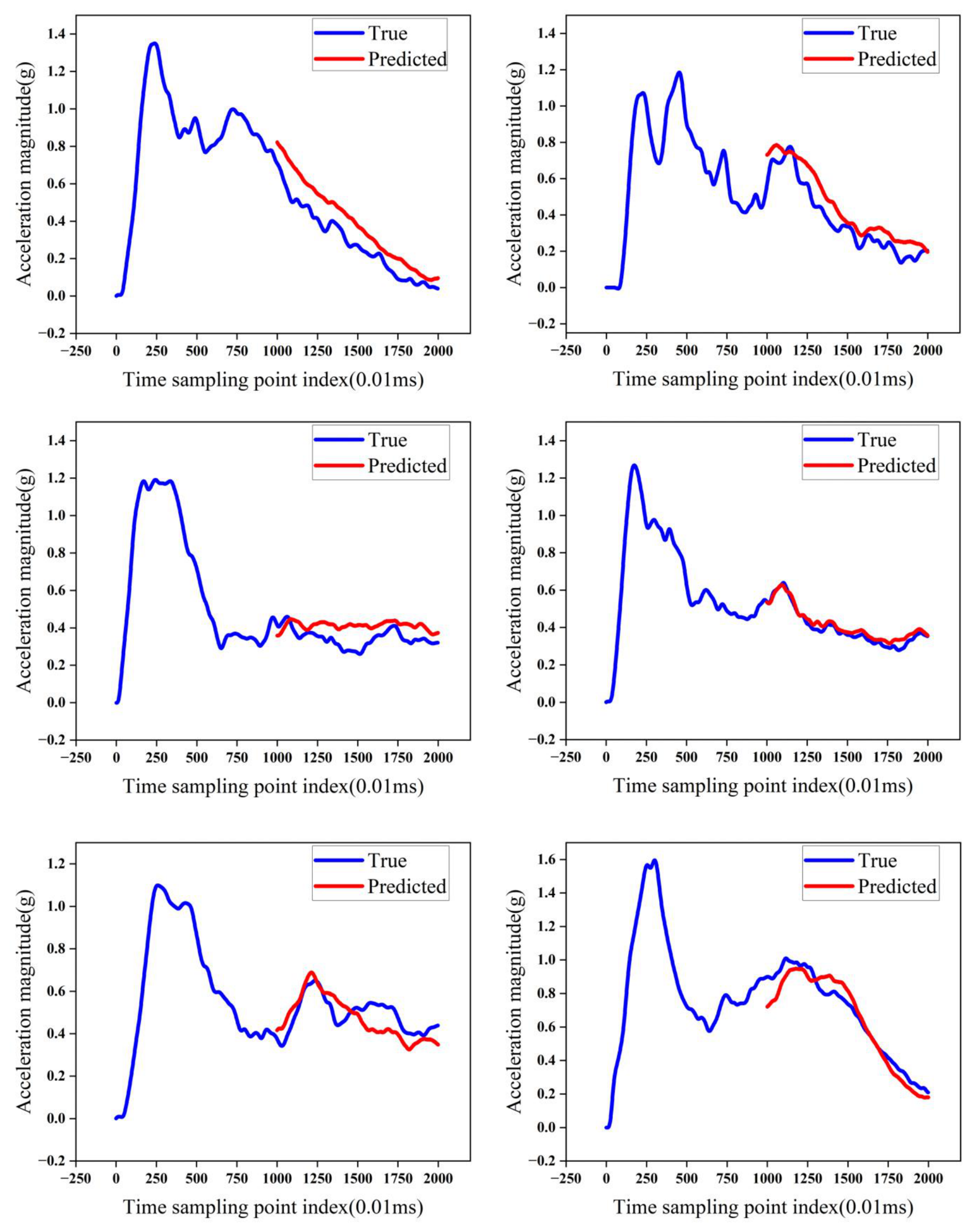
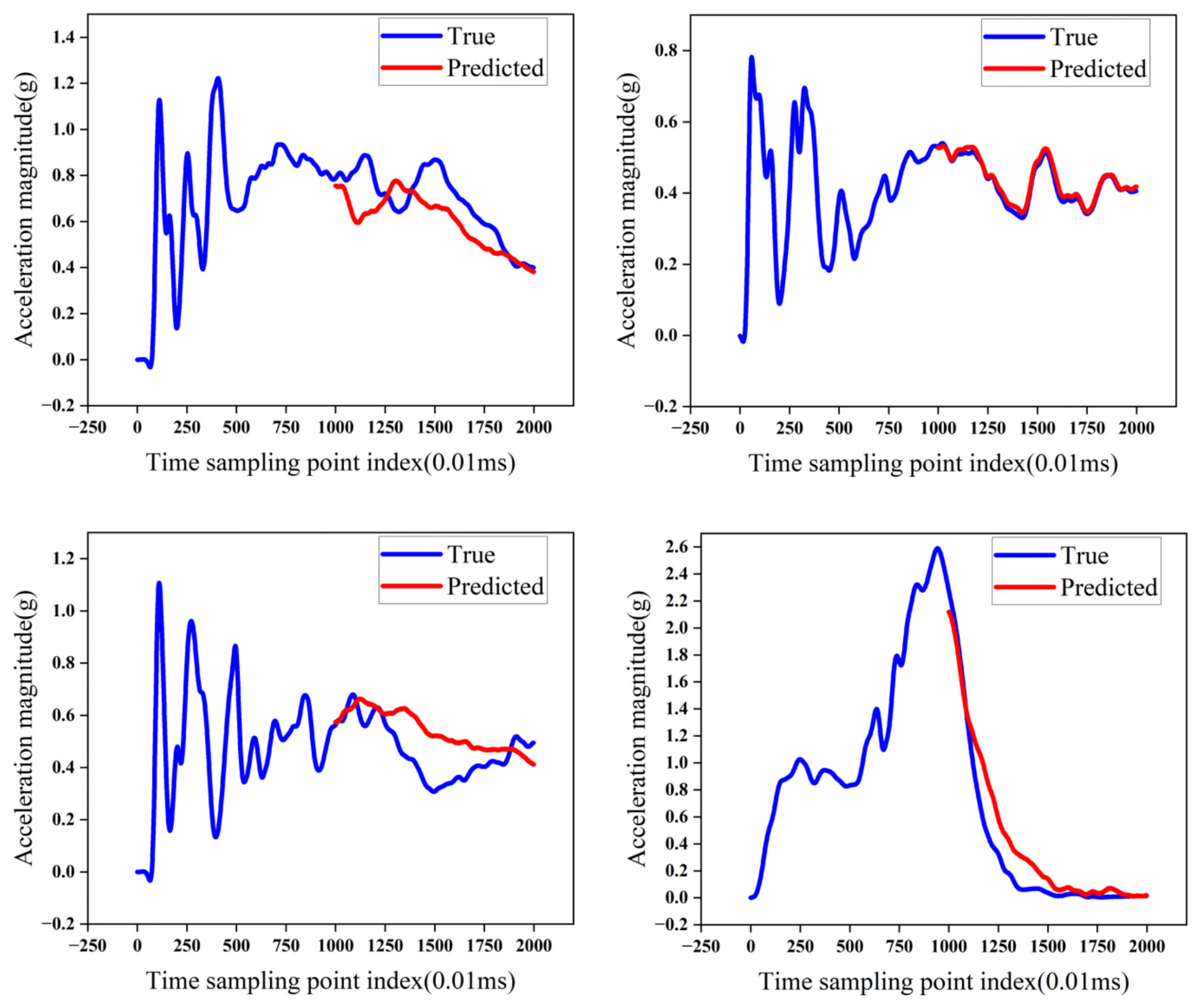
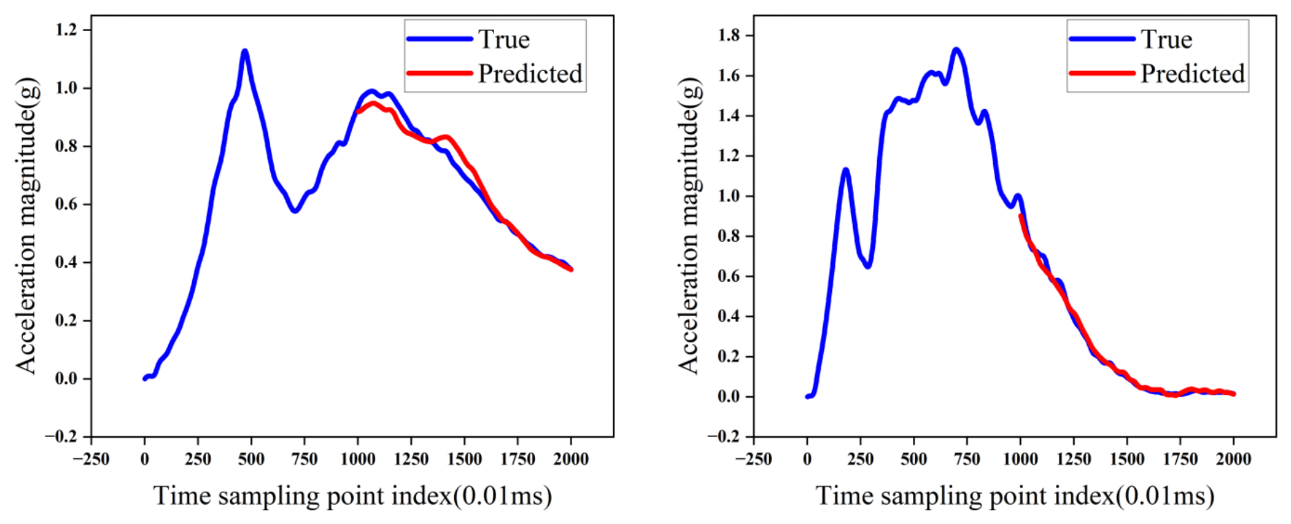
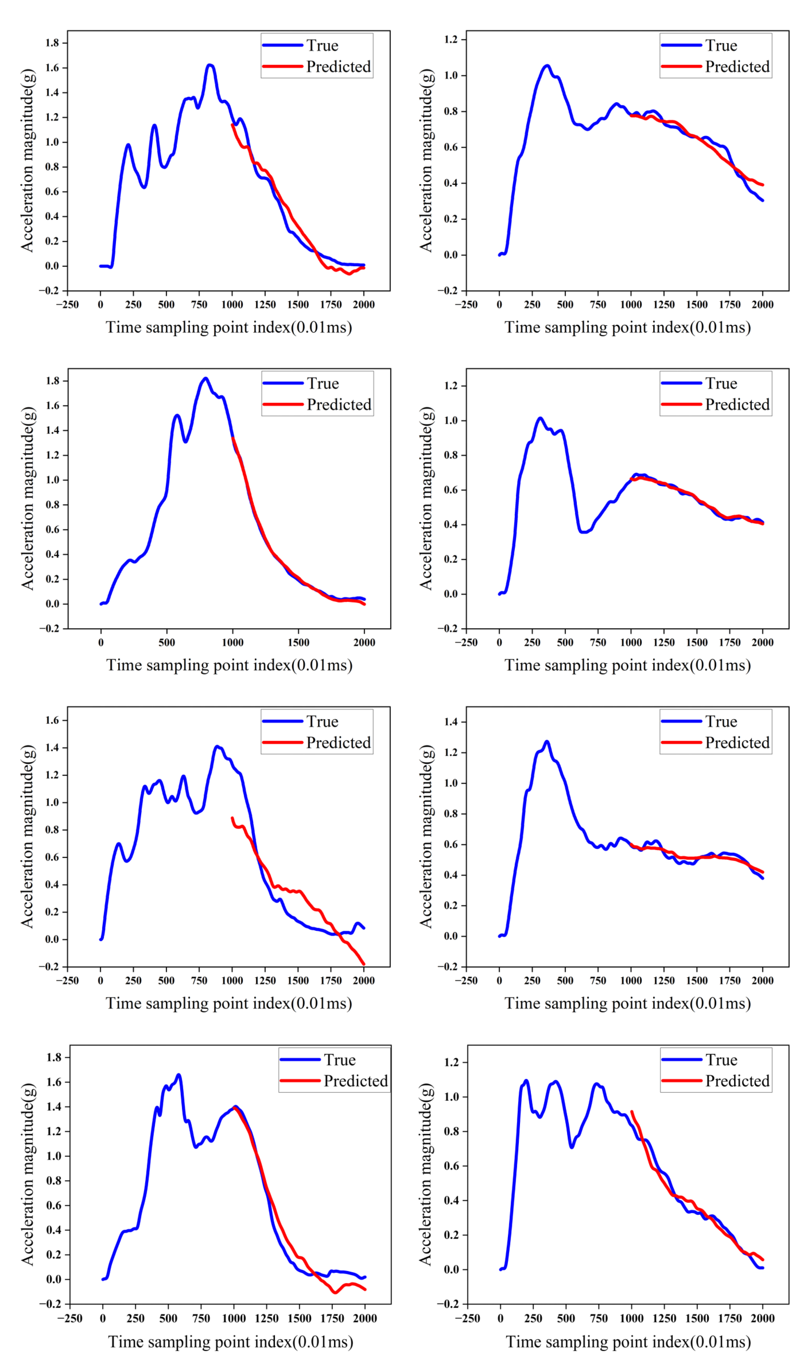
We visually examined ten representative test samples to compare the models under realistic crash dynamics. Each subplot shows the observed first half of the signal (time steps 0–999), the ground-truth second half (1000–1999), and the model’s prediction for that second half. This view makes it possible to compare the overall waveform and local transients.
For LSTM+CNN:
Figure 1.
Visual comparison of predicted rear-half acceleration curves for ten representative test cases — LSTM+CNN model.
Figure 1.
Visual comparison of predicted rear-half acceleration curves for ten representative test cases — LSTM+CNN model.
For TCN+GAN:
Figure 2.
Visual comparison of predicted rear-half acceleration curves for ten representative test cases — TCN+GAN model.
Figure 2.
Visual comparison of predicted rear-half acceleration curves for ten representative test cases — TCN+GAN model.
3.4. Visual Analysis and Comparative Evaluation of Prediction Performance
3.4.1. Visual Comparison of Model Predictions
Figure 3 compares the models’ predicted rear-half acceleration curves. Across the displayed crash scenarios, TCN+GAN follows the overall trend more closely and reproduces peaks more accurately. Each subplot shows the observed first half, the true rear half, and the corresponding prediction.
3.4.2. Error Distribution Comparison Between LSTM+CNN and TCN+GAN
We also compared absolute errors across the test set. For each time step in the predicted rear half, we calculated the absolute difference between the predicted and ground-truth acceleration values, normalized the errors to [0, 1], and pooled them across test cases. Figure 4 shows the resulting distributions.
In Figure 4, TCN+GAN’s errors cluster near zero, and most are below 0.05. LSTM+CNN’s errors are more dispersed, with a noticeable share above 0.1 and 0.2. Thus, although LSTM+CNN performs well on average, its predictions show larger local deviations. The TCN+GAN distribution also has a lighter tail, indicating fewer large errors—an important consideration when predicted signals are used to estimate HIC. The heavier tail for LSTM+CNN points to lower robustness when inputs are complex or highly variable.
Figure 5maps the average acceleration prediction error across the vehicle hood impact region for each model. Each pixel marks a measurement point, and its color indicates normalized error magnitude. Errors from TCN+GAN remain low across most of the region, while LSTM+CNN has localized areas of higher error, particularly near regions of greater deformation. This spatial view adds to the temporal error analysis and shows how performance varies with impact location.
Taken together, the concentrated, rapidly declining error distribution for TCN+GAN is consistent with stronger generalization and stability on this test set. This pattern accords with the model’s combination of long-range temporal modeling and adversarial training. On these measures, TCN+GAN provides the more reliable rear-half prediction, particularly across inputs with varied profiles.
3.4.3. Visual Correlation Between Predicted and True Values
Figure 6(a) and 6(b) compare predicted and ground-truth HIC values for LSTM+CNN and TCN+GAN, respectively. The dashed diagonal marks perfect agreement. TCN+GAN’s points lie closer to this line, indicating better agreement in the resulting HIC estimates. The signal comparisons also show that it preserves primary impact peaks, secondary rebounds, and terminal damping with less deviation across the tested crash scenarios.
LSTM+CNN captures the overall relationship, but its HIC predictions show more scatter, especially at higher acceleration levels. Errors in peak timing and magnitude, together with discontinuities where the observed and predicted segments meet, can leave late-stage high-frequency components underestimated. These differences may carry through to downstream safety metrics and contribute to HIC error.
3.4.4. Local Peak Preservation and Timing
Local peak height and timing matter when reconstructing the rear half of a signal, because brief, high-magnitude accelerations can strongly affect injury metrics such as HIC. Here we compare how well each model preserves extrema in the predicted segment.
TCN+GAN more closely retains the shape, height, and timing of prominent peaks. In high-impact cases with several rapid spikes, it reproduces primary and secondary impacts with little phase lag or attenuation. Its dilated convolutions may help it capture longer-range context while retaining fine temporal detail.
LSTM+CNN tends to smooth sharp changes and can delay or reduce peak responses. It reproduces broad trends, but is less precise about high-frequency peaks, especially near the boundary between the observed and predicted segments. Such errors can underestimate transient loads and affect later biomechanical analysis.
The measured mean absolute peak-timing deviation is 3.4 ms for TCN+GAN and 7.8 ms for LSTM+CNN. Mean peak-amplitude error is 0.045 g and 0.121 g, respectively. These results show that TCN+GAN more closely matches the timing and magnitude of local peaks in this evaluation.
Overall, TCN+GAN combines stronger numerical accuracy with better preservation of local waveform features, which can support crash-severity estimation and biomechanical evaluation.
3.4.5. Signal Smoothness and Physical Consistency
Beyond low numerical error and accurate peaks, a predicted post-impact acceleration curve should have smooth transitions, bounded amplitudes, and a decay pattern consistent with damping. These properties matter for biomechanical plausibility and regulatory assessment.
TCN+GAN’s outputs connect smoothly across the observed and predicted segments and reproduce the attenuation patterns seen in the crash data. The results suggest that the model has learned temporal structure that helps avoid abrupt artifacts; adversarial training may also discourage unrealistic outputs.
LSTM+CNN sometimes produces small discontinuities where the observed and predicted segments meet. It can also depart from the measured damping pattern, with sustained oscillations or delayed decay. These behaviors may reflect limitations in how the recurrent and convolutional components capture long-range and local signal features.
The average gradient deviation is 0.028 for TCN+GAN, compared with 0.074 for LSTM+CNN, indicating smoother predicted transitions under this measure. Zero-crossing-rate analysis also shows less high-frequency noise in TCN+GAN: its values are closer to the ground truth, while LSTM+CNN has a higher rate associated with residual oscillations.
Alongside its statistical performance, TCN+GAN produces acceleration curves that are more physically coherent in the evaluated cases. This quality is relevant when predictions feed into injury analysis, safety certification, or compliance assessment.
4. Conclusion
Across the quantitative metrics and visual comparisons, TCN+GAN more closely reproduces both the overall waveform and local transients. It also better retains the physical characteristics of the post-impact signals examined here, making it a promising option for injury prediction and crashworthiness assessment.
LSTM+CNN remains effective for signals with smoother, more regular structure. In the more dynamic crash cases, however, it is less reliable at capturing sharp transients and their timing.
For rear-half time-history prediction in this study, TCN+GAN is more accurate and produces more biomechanically consistent signals than LSTM+CNN. These findings support its further evaluation for automotive injury-risk analysis, regulatory testing, and design optimization.
References
- SHIN, G.; SONG, O. J. N. E.; TECHNOLOGY. A time-domain method to generate artificial time history from a given reference response spectrum [J]. 2016, 48(3), 831–9. [Google Scholar] [CrossRef]
- HAO, S.; DAEMI, S. R.; HEENAN, T. M.; et al. Tracking lithium penetration in solid electrolytes in 3D by in-situ synchrotron X-ray computed tomography [J]. Nano Energy 2021, 82, 105744. [Google Scholar] [CrossRef]
- ZHAN, Q.; BAI, C.; ZHANG, N.; et al. Feature extraction method of flow around airfoil based on time-history convolutional autoencoder [J]. 2022, 43, 526531. [Google Scholar]
- REDDY U, LAKHANPAL S, SINGH J, et al. Advanced Comparative Analysis of Time-Frequency Signal Processing Techniques and Machine Learning Models for Optimized Biomedical Classification; proceedings of the 2025 International Conference on Intelligent Control, Computing and Communications (IC3), F, 2025 [C]. IEEE.
- PRAVEEN, M.; DEKKA, S.; SAI, D. M.; et al. Financial time series forecasting: A comprehensive review of signal processing and optimization-driven intelligent models [J]. 2025, 1–27. [Google Scholar]
- DAS, M.; GHOSH, S. K. J. P. R. L. Data-driven approaches for meteorological time series prediction: a comparative study of the state-of-the-art computational intelligence techniques [J]. 2018, 105, 155–64. [Google Scholar] [CrossRef]
- YANG, H.; PAN, Z.; TAO, Q.; et al. Online learning for vector autoregressive moving-average time series prediction [J]. 2018, 315, 9–17. [Google Scholar] [CrossRef]
- YADAV, D. K.; SOUMYA, K.; GOSWAMI, L. Autoregressive integrated moving average model for time series analysis. In proceedings of the 2024 International Conference on Optimization Computing and Wireless Communication (ICOCWC); IEEE, 2024; Volume F. [Google Scholar]
- HONG, L.; CHENG, G.; CHUI, C. K. J. I. T. O. C.; et al. A filter-bank-based Kalman filtering technique for wavelet estimation and decomposition of random signals [J]. 2002, 45(2), 237–41. [Google Scholar]
- ZEN H, SAK H. Unidirectional long short-term memory recurrent neural network with recurrent output layer for low-latency speech synthesis; proceedings of the 2015 IEEE International Conference on Acoustics, Speech and Signal Processing (ICASSP), F, 2015 [C]. IEEE.
- DE SOUZA, V. L. T.; MARQUES, B. A. D.; BATAGELO, H. C.; et al. A review on generative adversarial networks for image generation [J]. 2023, 114, 13–25. [Google Scholar] [CrossRef]
- LI, D.; CHEN, T.; LIU, C.; et al. Semi-supervised GAN for enhancing electrocardiogram time series diagnostics [J]. 2025, 110, 108058. [Google Scholar] [CrossRef]
- HEGDE C, DASH S, AGARWAL P. Vehicle trajectory prediction using gan; proceedings of the 2020 Fourth International Conference on I-SMAC (IoT in Social, Mobile, Analytics and Cloud)(I-SMAC), F, 2020 [C]. IEEE.
- ELíA, I.; PAGOLA, M. J. E. A. O. A. I. Anomaly detection in Smart-manufacturing era: A review [J]. 2025, 139, 109578. [Google Scholar] [CrossRef]
- ZHANG, T.; WANG, W.; LI, B.; et al. Deep neural network based head injury criterion estimation for more efficient pedestrian protection performance evaluation in bonnet structure design [J]. 2025, 202, 103867. [Google Scholar] [CrossRef]
- SRIVASTAVA, N.; HINTON, G.; KRIZHEVSKY, A.; et al. Dropout: a simple way to prevent neural networks from overfitting [J]. 2014, 15(1), 1929–58. [Google Scholar]
- HUANG, F.; DENG, Y. J. N. N. TCGAN: Convolutional Generative Adversarial Network for time series classification and clustering [J]. 2023, 165, 868–83. [Google Scholar] [CrossRef]
Figure 3.
Visual comparison of rear-half acceleration predictions from LSTM+CNN and TCN+GAN across representative crash scenarios.
Figure 3.
Visual comparison of rear-half acceleration predictions from LSTM+CNN and TCN+GAN across representative crash scenarios.
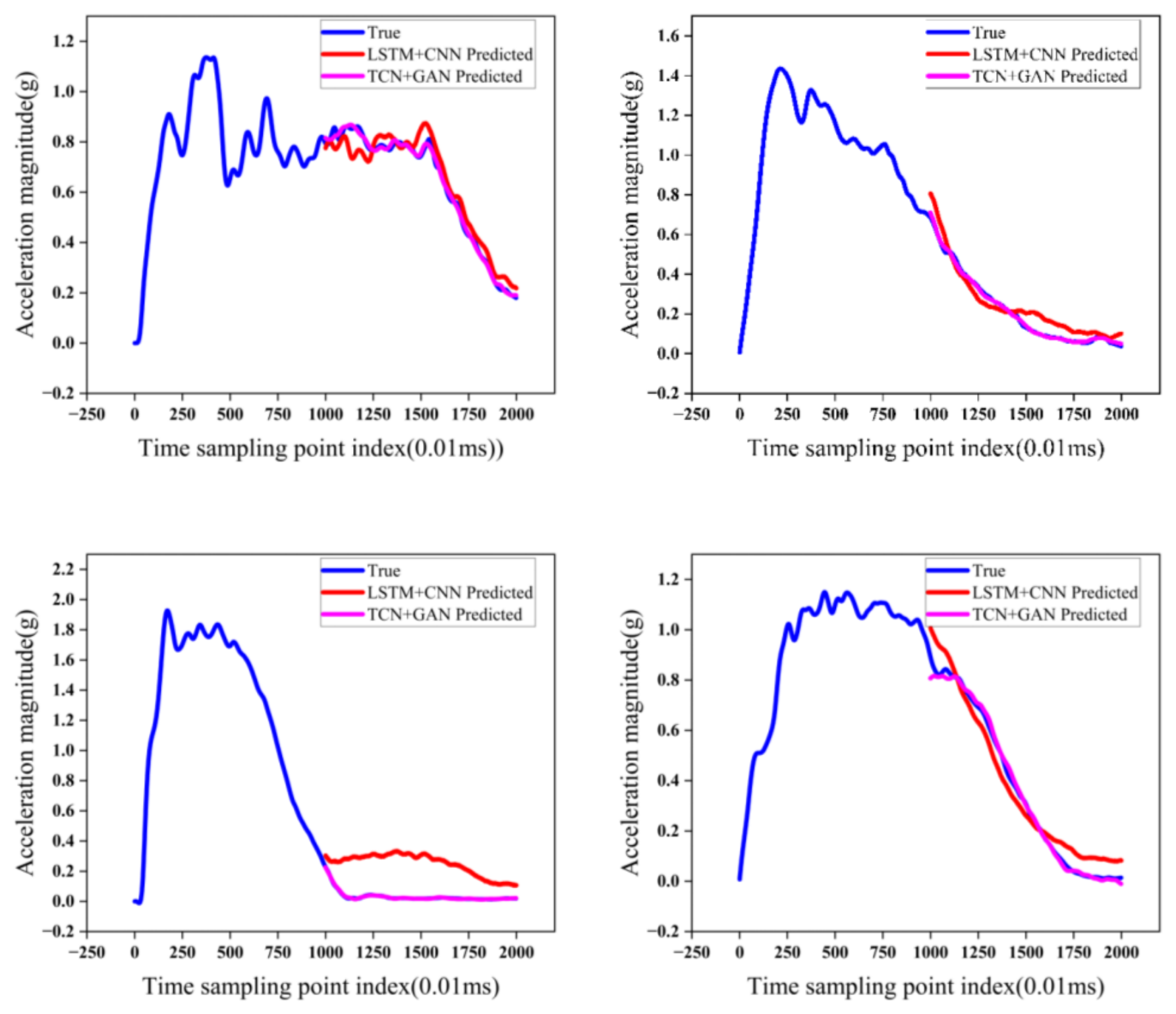
Figure 4.
LSTM+CNN vs TCN+GAN Model error distribution(0 to 100%).
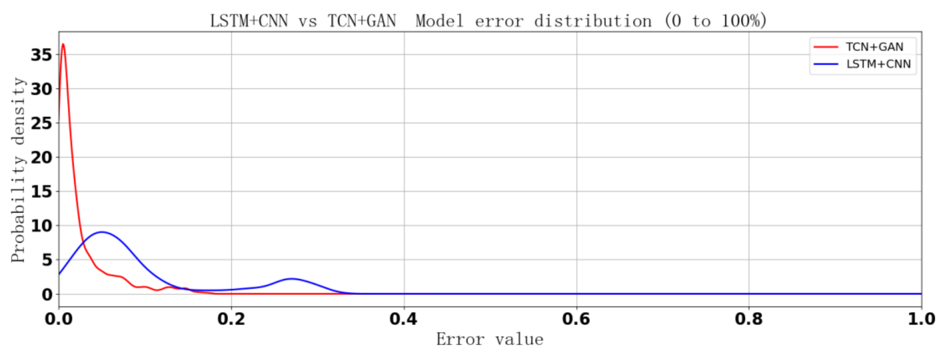
Figure 5.
Spatial distribution of average acceleration prediction errors on the vehicle hood impact region for LSTM+CNN and TCN+GAN models.
Figure 5.
Spatial distribution of average acceleration prediction errors on the vehicle hood impact region for LSTM+CNN and TCN+GAN models.
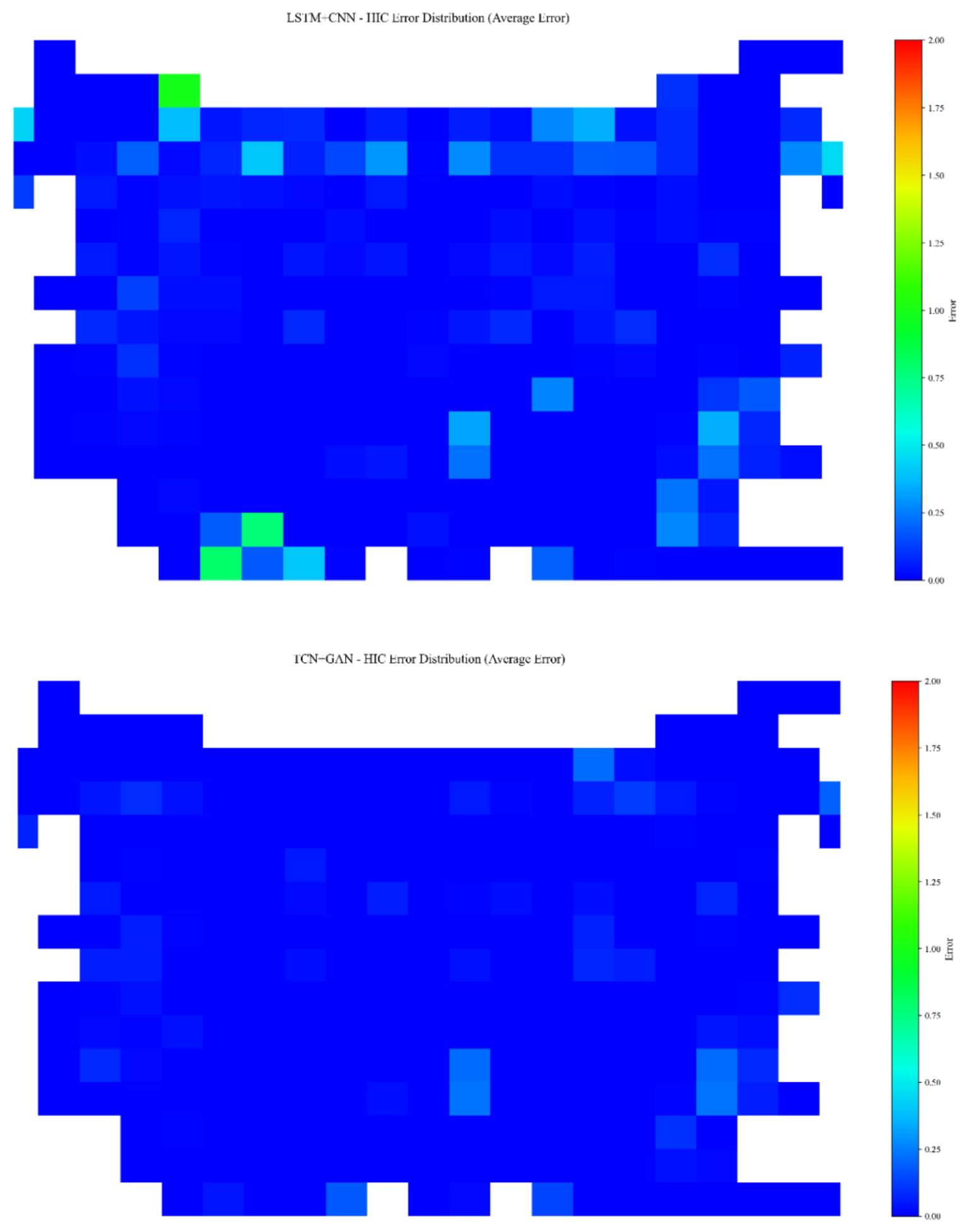
Figure 6.
(a). Scatter plot of true vs. predicted acceleration values for the LSTM+CNN model, with color indicating sample density. (b). Scatter plot of true vs. predicted acceleration values for the TCN+GAN model, with color indicating sample density.
Figure 6.
(a). Scatter plot of true vs. predicted acceleration values for the LSTM+CNN model, with color indicating sample density. (b). Scatter plot of true vs. predicted acceleration values for the TCN+GAN model, with color indicating sample density.
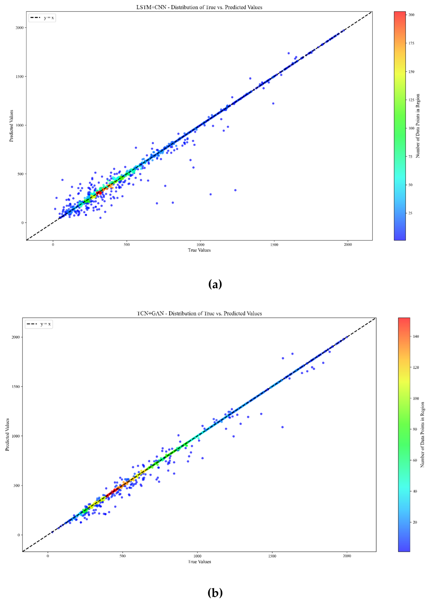

Table 1.
Performance comparison for rear-half time-history curve prediction.
| Model | RMSE | MAE | R2 | DTW | HIC Error (%) | |
|---|---|---|---|---|---|---|
| LSTM+CNN | 0.0387 | 0.0263 | 0.963 | 0.142 | 2.67 | |
| TCN+GAN | 0.0331 | 0.0227 | 0.972 | 0.127 | 1.85 |
Disclaimer/Publisher’s Note: The statements, opinions and data contained in all publications are solely those of the individual author(s) and contributor(s) and not of MDPI and/or the editor(s). MDPI and/or the editor(s) disclaim responsibility for any injury to people or property resulting from any ideas, methods, instructions or products referred to in the content. |
© 2026 by the authors. Licensee MDPI, Basel, Switzerland. This article is an open access article distributed under the terms and conditions of the Creative Commons Attribution (CC BY) license.
Copyright: This open access article is published under a Creative Commons CC BY 4.0 license, which permit the free download, distribution, and reuse, provided that the author and preprint are cited in any reuse.