

Submitted:
24 October 2026
Posted:
26 October 2026
You are already at the latest version
Abstract
Autism Spectrum Disorder is fundamentally arrested neurodevelopment impacting the somatic sensory motor systems with underlying multifaceted and tractable causal factors, spanning from genes to complex social interactions. Mounting peer-reviewed scientific evidence shows profound differences in cardiac, smooth, and striate muscles with associated genes, suggesting causal links to motor systems. A less explored aspect of these muscles’ dysfunctions, in the context of interventions, is the quality of the returning afferent stream created by self-generated movements. Although defined as a deficit in social interactions, very seldom we find methods that address the basic social unit, the dyad, and the connection, or the lack thereof between the two agents, as the autistic person interacts with a caregiver, practitioner, diagnostician or educator. Here we use the Torres agentic learning (TAL) approach to objectively quantify dyadic interactions in the context of self-initiated, uninstructed learning, recruiting spontaneous movements, minimizing prompted goals and maximizing the conditions for pleasant surprises leading to self-discovery of salient sensory goals. We integrate TAL with the Anat Baniel Method® Neuromovement® (ABMNM), the latter providing nine essential principles empirically derived to guide the intervention. ABMNM builds awareness through child-practitioner’s coupled movements, while TAL provides principled standardized ways to measure the outcomes. Combining ABMNM, biosensors and TAL into the daily workflow of a public, mainstream school setting, we tracked the evolution of three cases of ASD over 4 months. Transfer entropy metrics revealed (across the nodes of the body) initial leading by the child, setting the stage for later lead of the practitioner as in an interchanging dance. These patterns were accompanied by increased signal to noise ratio and higher predictability and motor fluidity. They were consistently found when comparing pre- and post-therapy states, but also throughout the continuous session. We offer standardized digital biometrics to capture learning outcomes at different time scales spanning from minutes, hours, weeks, to monthly latencies, informed by performance rubrics involving the ABMNM nine essentials. Besides motor gains, we report unexpected, functional outcomes signaling improvements in cognitive and social performance.
Keywords:
autism
; spontaneous movements
; agentic learning
; awareness through movement
; kinesthetic reafference
; dyadic interactions
; functional goals
1. Introduction
The quality of spontaneous movements is key to the development of neuromotor control [1]. Before birth, spontaneous random motions mediated by central pattern generators (CPGs), involuntary muscle contractions and reflexive motions inform physicians about fetal health and can be monitored through ultrasound and fetal magnetic resonance imaging (fetal MRI) [2]. After birth, their evolution throughout the first 30 weeks, an intense period of growth and neural development, informs us of the health and progression of the nervous systems’ highly complex, nonlinear dynamics [3].
During infancy, we can assess the quality of spontaneous movements using the principles of the Prechtl General Movement Assessments [4,5,6]. We can also track the early evolution of accompanying reflexes, found to flag atypical neurodevelopment when missing important milestones [7,8,9,10]. As these bodily motions evolve through weeks 9-20 from writhing movements to fidgeting movements, and as they transition by weeks 15-30, to antigravity, intentional movements, they can reveal a schedule of healthy development of neuromotor control or forecast impending sensory-motor issues [10,11,12,13] (Figure 1). More generally, tracking the micro-movements of voluntary actions [14,15,16] and their spontaneous counterpart [17,18], can reveal important scaling power laws capturing maturational milestones of motor variability across the human lifespan, or flagging their absence in autism spectrum disorders [19].
Because throughout various neurodevelopmental stages, spontaneous movements fold within voluntary movements [21], they transpire largely beneath awareness. They bypass the naked eye of an observer and even escape full awareness of our reafferent kinesthetic sensations. As such, they become difficult to spot, track, or altogether study. Our lab discovered spontaneous movement segments embedded in the complex bodily actions of competitive athletes performing martial arts routines [22,23] and the tennis serve [24]. We were then able to characterize their stochastic signatures in autism [16,21], Parkinson’s disease [25,26,27], stroke [28], deafferentation [29] and schizophrenia [30], providing in each case, a desirable motor target for treatments under a common unifying statistical platform for individualized behavioral analysis [31] and under the Torres’ agentic learning (TAL) model [18]. TAL is precisely designed for autism. It minimizes the prompting of goals (which increases the uncertainty of their motor systems). It favors instead maximizing the conditions for naïve, free-form exploration, as a self-regulatory mechanism opening the brain to experiencing pleasant surprises that help modulate the system’s arousal states. This process leads to a series of steps that result in the self-discovery of novel outcomes. These include salient sensory stimuli perceived and enacted without instructions [18].
Despite acknowledging the importance of spontaneous movements in neurodevelopment [11,12], and their key role in the detection and treatments of nervous systems disorders [18], up to now, interventions that address spontaneous movements and improve their quality in the context of agentic, exploratory motor learning are scarce. In particular, it is hard to find versatile therapies that help athletes, musicians, and dancers alike, with the same ease as they can help patients with Parkinson’s disease (PD), those recovering from a stroke, infants or young children with cerebral palsy and those on the broad spectrum of autism/ADHD -the focus of our collaborative work here.
The Anat Baniel Method®NeuroMovement® (ABMNM) is a type of intervention that leverages spontaneous movements, including random and reflexive motions of young neurotypical infants often retained in autism well beyond infancy [32]. ABMNM aims at enhancing movement awareness without deciding a priori what goals to give the child. Instead, the practitioner meets the child’s neuromotor systems where they are. Rather than trying to “fix” the child, they connect with the child and utilize what the child is doing as the basis from which, through small motoric variations, spontaneous differentiation emerges. Upon creating the proper ecological conditions then learning unfolds with the same wondering awe that a newborn possesses during the early, naïve stages of neurodevelopment. This method is mediated by the practitioner-student dyad attuned, dynamic interactions. The practitioner initiates, through contact, connection with the child. Movement-based, randomized activities ensue, while considering both the child’s responses and the state of the child’s system in the moment. Practitioners and students embark on a journey mediated by naïve fascination and wondering, that is nonetheless highly informed by the practitioner’s experience. This initially seemingly aimless process soon transitions to mutual exploratory learning, resulting in the child’s self-discovery of salient sensory goals for purposeful action.
This process builds skillful and effective ways to move, sense, emote, learn, think and more broadly, interact with the world through nine essential principles [33] (presented in the methods section). The person increasingly becomes self-aware of their body in motion and learns to direct it, first as “one body”, and “one brain”, and then as a dyad, together with the teacher Through rapid, small changes the spontaneous learning that ensues between the child and the teacher shows recognizable developmental milestones. Much like an infant who meets the motor milestones, the person learns to move independently, with a functional, vitalized sense of kinesthetic reafference [34]. This development also brings contextual awareness that translates into improvements in social interactions at the classroom and the home environments.
As in a harmonious dance, the spontaneous rhythms emerging from the dyadic interactions between the practitioner and the participant, interactions that emerge from where the recipient is at present, help the person find emerging predictable patterning in voluntary movements—a form of self-discovery of action-consequences that leads to a sense of action ownership and the expectation to learn. The interactions bring intrinsic satisfaction as the person learns to sense and accurately predict the consequences of his own self-generated motions, partly evoked by the motions of the teacher. In the words of von Holst and Mittelstaedt [35], “Voluntary movements show themselves to be dependent on the returning stream of afference which they themselves cause”. The returning, consequential stream emanating from the spontaneous segments of our actions is brought up to awareness using the NeuroMovement® method. But in a rather unique way, this is done without obfuscating the natural role that such open-ended movements play since infancy, on the emergence, shaping and continuous support of voluntary motor control.
Leveraging Spontaneous Segments in Our Movements
As spontaneous segments embedded in our shared rhythms are subtle, slower and goal-less, they can be key to evoking awareness of desirable outcomes, without the pressure of fulfilling some preset expectation by an external agent that would only heighten uncertainty in the system and bring anxiety to both the person and the practitioner. Spontaneous segments of our movements can play a fundamental role in dampening the high levels of noise present in self-initiated voluntary actions aimed at discovering the end goal of a task [18]. In dyadic settings, they may serve to evoke the notion of action ownership, increasing the sense of motor autonomy and socio-motor agency [36]. Indeed, several experimental settings [16,18] have demonstrated that spontaneous movements in autism are not only more malleable than intentional, goal-directed ones, but more importantly, they are within normative ranges —unlike the spontaneous action segments of patients with PD [26] or patients with schizophrenia [24,30].
Here we harness the spontaneous, uninstructed movements evoked by ABMNM in the context of student-practitioner dyads, where one member of the dyad is autistic. Not only did we longitudinally track the outcomes throughout the child’s and the teacher’s shared bodily motions, we also did so through the lens of the parents and teachers, as they reported on the profound changes in the child’s social life, cognition, and reduction in anxiety, confusion, and rage. In an unprecedented manner, we objectively quantified the dyadic interactions during ABMNM learning and extracted, longitudinally, the individualized effectiveness of this intervention. Using objective biometrics, we followed the spatio-temporal interplay of this evolving movement-sensing dyadic dance across multiple frequency bands, co-registered from their joint biorhythms to facilitate reproducibility and scalability of this intervention.
2. Methods
2.1. Participants and Context
Three children, two 6 years old and one 12 years old, all with a diagnosis of autism spectrum disorders participated in the study. Two are males and one female. The public school where the study took place was mainstream. The children with the ASD/ADHD diagnosis were integrated but provided with the usual individualized aid’s support within a regular classroom. This integration was not working out as planned, which motivated bringing ABMNM to the school.
| Student | Age | Sex | Dx |
| A | 6 | F | Sensory Processing Disorder, Somatic dyspraxia, Severe language delays, apraxia of speech, general difficulties with motor planning and execution, problems processing information, cannot perform complex sequential tasks. |
| C | 12 | M | ASD-ADHD. Teachers report that he progressed in full day classes and is proficient in academia however, his teacher and parents report that he struggles with emotional regulation and gets overwhelmed easily when others do not follow ‘rules’ and the environment is chaotic. |
| E | 6 | M | Sensory Processing Disorders and suspected ADHD (undiagnosed). Teachers report: Intelligent but difficulties focusing and sustaining attention, at times hitting others to get other’s attention. |
The longitudinal study took place in the span of 4 months with a schedule consisting of an intensive block of 10 sessions, 5 days in a row, whereby 1 session was administered by 1 practitioner in the morning, and another session was administered by another practitioner in the afternoon. This is important for motor generalization and transfer, to prepare the child for real social situations with variations in interaction styles.
At the completion of the intensive block, a period of 4 months followed with sessions set at 4 lessons / month done over 2 days. A total of 25 sessions were collected for each child using this intensive vs. tapering off intensive regimes. ABMNM appreciates the rapid changes in the intensive block and tracks the fluctuations in the tapering off intensive block. Digital implementation of this method was achieved with wearable biosensors to ascertain the outcomes of the intervention and the effectiveness of the dyadic interaction, while observing the nine essential principles of the intervention methodology.
2.2. Instrumentation
The APDM advanced wearable biosensors, Opals (Clarion) were used in this study. Twelve sensors, 6 on the child and 6 on the practitioner (for each dyad) were located as indicated in Figure 2. The Opals are light-weight inertial measurement units sampling at 128Hz and registering triaxial acceleration through accelerometers and triaxial angular velocity through gyroscopes. Temperature and magnetometer data were also registered but will not be reported on the paper. The sensors were affixed to the person with elastic straps and did not interfere with the clothing or the motions. They pose no risk, and their use of research was approved by a private IRB in accordance with the Helsinki Act). The study, which took place at a school was approved by the school and parents provided informed consent according to their own IRB. We analyzed the deidentified biosensor data under Rutgers University IRB Pro2018000141 approved on 5/29/2018 when the study ended, due to the COVID 19 pandemic.
Bodily locations were on the thorax (sternum), lumbar, wrists and feet (as depicted in Figure 2). The mobility lab was used to acquire data synchronously from all 12 Opals and saved as coma-separated value (CSV) files for further processing of the column-wise time series. Videos of each session were obtained from two viewpoints using GoPro cameras and an additional Cannon camera on a tripod recorded the sessions. At the start of each session, parents and schoolteachers were summoned to the room before the child came in from class to do the session. They were interviewed through open-ended questions, to report on daily progress and challenges. The answers obtained were then examined in relation to contextual situations beyond the focus of the intervention. These included changes in sleep patterns, food intake, changes in conversational patterns, and socialization at school and in the home environments.
Methods to obtain acceleration and angular speed were developed in-house using MATLAB (MathWorks) along with algorithms to analyze and interpret the time series data from the sensors (further described below).
2.3. The Nine Essentials in ABMNM
The intervention follows The Nine Essentials which Anat Baniel empirically identified after 20 years of practice [37]. During those years thousands of children attained outcomes well beyond their original prognosis. She derived nine underlying principles defining the “how to” intervene to potentiate the child’s ability to learn. Then these nine essentials became the core foundation of a pedagogical tool used to scale the method worldwide to hundreds of practitioners today, including physical therapists, occupational therapies, teachers, physicians, among others [33,34].
- Movement with attention to the feeling of self: Movement is life, present in all actions and behaviors. We posit here that movement is central to the growth and development of the brain, i.e., to all learning. However, movement by itself is not enough. Rote repetitions of movements seeking to accomplish an externally prompted goal will only tend to reinforce already existing patterns. Learning and positive change requires that the child brings their attention to the sensations associated with their movements, to what they feel. Introducing movement to the child in ways that spontaneously brings them to feel their own movements, facilitates internal motor-sensory communication in ways that potentiate and upgrade the functioning of their brain.
- Slow: Fast, we can only do what we already know. To learn and master new skills and overcome limitations, we need to slow way down. Slow gets the brain’s attention in a deliberate way. This in turn helps the brain notice differences, sense, and feel, i.e., generate and experience new information. Purposely slowing movement down in the child requires that the practitioner, therapist, teacher, or parent slow themselves down, so they can feel and connect with the child’s and the adult’s individual networks into one fully interconnected network. In this global network, the practitioner can lead or be led by the child.
- Subtlety: A powerful way to enhance the ability of the child’s brain to perceive differences and usher in spontaneous learning, is to reduce the force, or the intensity of stimulation with which we interact with, or impose on the child,—physically, emotionally, and cognitively. This in turn enhances both our own and the child’s ability to feel, sense, and notice, thus providing the brain with new, progressively more refined information to learn successfully, grow and change with.
- Variation: Variations are necessary for learning. Variations are given differences to be perceived. Generating variations, we hypothesize, are a built-in feature of the brain, e.g., central patterns generators (CPGs) from the brainstem provide subtle variations that we can observe in movement beginning in utero and continuing after birth during neurodevelopment. More generally, variations are an immediate and easy way to intentionally wake up the brain and help the child become a potent learner. Variations can be generated by varying actions, speed, size, direction, content, context, affect, and intensity in relation to where the child is, rather than in relation to preconceived goals. They can come in the form of play, “making mistakes”, creativity or exploration. They make learning possible and fun.
- Enthusiasm: Enthusiasm is not us clapping, cheering, or saying “good boy/girl” or “good job” when they perform to our liking. We leave it to the child to notice, to own their experience. We don’t highjack it from them. For us the enthusiasm and recognition of the child’s changes need to be an internal, quiet process. We choose to internally amplify our delight in response to seemingly small as well as big changes in the child. This internal amplification is felt and perceived by the child and further potentiates their learning and enhances their own agency.
- Flexible goals: There is nothing wrong with wanting the child to achieve what will provide them with eventual autonomy, independence and hopefully a satisfying life. Yet there is no way to know in advance, the exact, or even the approximate path that will lead the child to reach these goals. With flexible goals we look to create conditions that will help the child and their brain generate the underlying processes through which learning takes place in an organic, spontaneous way, the way newborns, infants, and children typically learn. Setting a priory rigid goals for the child and attempting to force the child to perform neurotypically will further confuse and alienate the child from themselves and their surroundings. It will further groove in their limitations and lead to failure and trauma. Our intention is to help the child become a potent learner where the specific content and timing of the learning is to be discovered, just like with a healthy infant.
- The learning switch: At any given moment the brain is either in a learning mode –the learning “switch” is on—or not. All the above Essentials help wake up the brain and turn the learning switch way up. You know that the “switch” is on and the dial is way up when the child spontaneously pays attention, is alert, shows interest, delight, and initiates their own involvement. And then they are done for a while; the learning switch is off and we need to stop. In our experience of over 40 years of practice, we have found that usually a potent state of learning for the child Is between 20-30 minutes. Another session may be offered later in the same day. A third session, however, is not useful as it just exhausts the child.
- Imagination and dreams: Einstein said: “Imagination is everything. It is the preview to life’s coming attractions.” Imagination is freedom and a resource that the practitioner is invited to utilize. With a child around 3 years old or older, the conditions can be created by the practitioner for the child to imagine. In ABMNM we often utilize imagination as part of the intervention. Imagination, like all other skills, can be developed and enhanced, contributing to the child’s ability to learn. Dreams: Children, from a very young age have wishes, desires, wants, preferences—the equivalent of having a dream. Connecting with the child and allowing, when appropriate, for their preferences to be included in the process, greatly enhances the outcomes.
- Awareness: In ABMNM awareness is an action. “Awaring” in relation to the self is the action of self-discovery that spontaneously self-emerges from the interaction between the practitioner and the child during the session. It is an integral part of and driver of learning and development at any age and greatly enhances the integration of newly emerged capabilities. This act of self-realization of one’s own body then extends beyond the session and out into the world. It may occur at any given moment during the session, yet it has a long-lasting transformative effect on the child, which the ABMNM practitioner is trained to recognize, join, follow and dance with.
The schedule of lessons in ABMNM is comprised of an initial period coined “the intensive”. It usually lasts between 1-2 weeks, occasionally longer and has 2 daily sessions, up to 45 Minutes each, 5 days per week. In this period there is appreciable rapid change, followed by a period of anywhere between two weeks to a couple of months, tapering off in frequency as the child develops increased functionality, spontaneous learning, agency, and independence. This (tapering off intensive) period is aimed at integrating and stabilizing the initial rapid changes into the motor stream, and to broaden the repertoire of the child’s goal-directed movements, and their variations. It is conceived as a period of consolidation towards enabling continued sensory/motor differentiation and motor-action fluidity [37].
As the child’s sense of action ownership and overall motor agency develops, lessons are less frequent, or terminated, unless disruptive, highly stressful, or traumatizing life events call for renovated intensive sessions. Puberty, strokes, and accidents are amongst life events that would return the person to renovated intensives.
During the present study, at the start of each session, parents and teachers from the child’s school where the study took place, were briefly interviewed (using open ended questions) to ascertain if they saw anything different in the child’s behaviors and capabilities at the home and at the classroom environment. The interviews were videotaped as were the sessions. We report the results of the interviews in the Supplementary Materials.
2.4. Standard Protocol for Pre- and Post Assessment of Change
In addition to the interview with parents and teachers at each session, we obtained pre- and post-therapy measurements of standardized tasks designed by our lab to measure volitional control [38]. These tasks are commonly used as part of our research studies and protocols to evaluate neurological movement disorders. We reasoned that since the ABMNM relies primarily on spontaneous movements and avoid instructed goals, it was important to measure offline, before and after the session, the ability of the person to have volitional control over self-generated actions and do so when the actions were performed in tandem with the practitioner. The tasks gave us a standardized way to measure progress and the effectiveness of the intervention, i.e., in addition to the continuous measurements taken during the intervention. The interventions were more variable and had unexpected turns, tailored to the child-practitioner evolving interactions. Because of the inherent variations in the ways in which the practitioners perform the intervention in an individualized manner, the standardized tasks served as an anchor to provide, from session to session, a controlled measure of change and progress. We report on both summary metrics across all sessions and sensors, and unfolding trajectories of the stochastic parameters of interest.
The tasks were performed in the following (deliberate) order of complexity: (i) Laying down at rest while trying to remain still. This task is designed to measure the ability of the person to have volitional control over the body, while deliberately suppressing involuntary motions. (ii) Pointing to a visual target. This task is designed to measure variations due to both goal-directed motions to a target and spontaneous retractions from the target towards rest or in transitioning motions to other goal-directed segments. (iii) Sit to stand. This task provides a sense of full body control during the lifting phase (against the direction of gravity) and the sitting phase (toward the direction of gravity). Variations are contributed from both segments and as in the other tasks, we hypothesized that there would be reductions in the variance of fluctuations in the linear acceleration (displacements) and angular speed (rotations) of the body.
The three standard tasks were performed by the child in tandem with the practitioner, and each task repeated within the span of 1.5 minutes, totaling approximately 4.5-5 minutes, before and after the session. Sessions lasted a minimum of 30 minutes but could reach a full hour, depending on the child’s predisposition. Continuous recordings of the session were also registered and analyzed. Figure 3A shows the room where the interviews took place. Figure 3B-E show examples of the three standard tasks used pre- and post-session. Figure 4 shows an example of continuously registered sessions where the practitioner helps the child build awareness of his self-generated movements via moving with attention, instead of specifying instructed goals. These examples (from head to toe) build variations of motion through haptic feedback and subtlety in the slow motions that the child senses back. In a give-and-take dance of both passively moving the body of the child, with attention to his self-generated motions, as the child actively reacts to them with cognizant thoughts of his own motions, the child builds awareness of different body parts and eventually carves out new locations on the body schema that were inexistent on this map prior to the therapy. Likewise, the practitioner learns with the child, gently guiding this exploratory learning, and steering the process without interfering with its natural flow.
2.5. Analysis of Digital Data
2.5.1. Stochastic Analysis: Micro-Movements Spikes and Gamma Process
The time series of triaxial linear acceleration and triaxial gyroscopic motions representing rotations were converted to acceleration (m/s2) and angular speed (rad/s) respectively, using the Euclidean norm of the three-dimensional acceleration vector and three-dimensional angular velocity vector, respectively (Equation 1).
Here a represents the acceleration vector with components along the x, y and z axes. Figure 5 explains the analytical pipeline to obtain the micro-movement spikes from the original time series of linear acceleration (m/s2) and angular speed (rad/s). This is done for one-minute-long sliding windows with 50% overlap, such that 128 frames per second x 60 seconds provide 7,680 frames to perform empirical estimation of stochastic parameters. This contrasts with assuming theoretical distributions (e.g., the Gaussian distribution) to compute the moments and to provide summary statistics of the data, such as grand averages leading to a one-size-fits-all approach. Furthermore, in a truly personalized manner, the parameters of interest are normalized to account for the individual anatomical features of the participant and to perform analysis of standardized ranges across participants. These analyses are performed for each agent of the dyad, i.e., the student and the practitioner, since their limbs have disparate anatomical lengths confounding the ranges of motion. The micro-peaks from the micro-movement spikes (explained next) scale out such allometric effects and provide a true standardization of the kinematic parameters.
Briefly, for each participant and each of the 12 sensors, the peaks of the time series are obtained (Figure 5A). The frequency histograms of the peaks are subject to probability distribution estimation analysis, using maximum likelihood estimation (MLE) with 95% confidence intervals. The continuous Gamma (Г) family of probability distribution functions (PDF) is found to fit best the frequency histogram of the peaks (Figure 5B), in an MLE sense. Thus, the Gamma shape (a) and scale (b) parameters are obtained along with the first and second moments, the Г-mean and Г-variance, Γμ = a ⋅ b and Γσ = a ⋅ b2
The points on the time series are then subtracted from the empirical Г-mean (Figure 5C). The absolute values of the difference between each frame and the Г-mean are normalized to account for allometric effects (anatomical disparities in body length) that impact the ranges of the values of the kinematics parameters of interest. This is attained with Equation 2.
The micro-movement spikes (MMS) are obtained on the left-hand side of Equation 2. Here Peak represents each peak of the time series of absolute deviations from the Г-mean. The two local surrounding minima of each Peak are obtained, such that the average of all points from local minima to local minima (including the Peak) is obtained at each local peak. This is the new series of peaks that are standardized to scale out allometric effects due to anatomical disparities across participants (Figure 5D). The standardized micro-peaks are then used to obtain once again the frequency histograms of the micro-peaks and find the best continuous distribution family fit, in an MLE sense, with 95% confidence. The continuous Г family turned out to be the best fit of the micro-peaks from the MMS derived from both the linear acceleration and the angular velocity time series. Figure 5E shows the Gamma shape and scale parameters with corresponding 95% confidence intervals involving one participant in Pre- and Post-measurements using the motions from one of the tasks from the standard protocol described in Figure 3.
These Г-parameters of the MMS obtained and plotted on the Г-parameter plane as points (a, b) with 95% confidence intervals (Figure 5E) serve as the basis to obtain the Г-moments and derive other parameter spaces representing different aspects of the data. Examples are shown in Figure 5G (the Г-moments) and Figure 5H (the Г-NSR vs. the Г-skewness), both having empirical interpretation from sampling across thousands of cases across the human population. Importantly, the MMS at zero values are those with zero deviation from the empirically estimated Г-mean, which we locally track, minute by minute, during the session. This is done for the student, for the practitioner and for the shared space spanned by the cross-coherence of their micro-peaks from the MMS time series.
Empirical Interpretation of the MMS and Г-process: The Г-parameter plane has been studied in autism by our lab across thousands of participants, ranging in ages from toddlerhood to adults in their sixties. It has also been well characterized in other disorders of the nervous system and in neuropsychiatric conditions (e.g., Parkinson’s disease [39], deafferentation [27,40], essential tremor [41], Fragile X [42], SHANK3 deletion syndrome [24,43], schizophrenia [30], among others) as well as in neurotypical controls since birth and throughout the lifespan. These studies have comprised both longitudinal and cross-sectional scenarios. They have revealed that fluctuations of the points on the Г-parameter plane tending to the exponential range of the Г-PDF characterize dysregulated nervous systems whereby the Г-scale parameter signaling the dispersion of the Г-PDF is abnormally elevated. The Г-scale parameter represents the Г noise-to-signal ratio (Г-NSR), since and the Г-shape (a) is related to the Г-NSR (b) according to a scaling power law [16,21] whereby as the Г-NSR decreases, the Г-shape increases towards the Gaussian ranges of the Г-PDF. Conversely, as the Г-NSR increases, the Г-shape decreases towards the memoryless exponential range a = 1 of the Г-PDF. This empirical result helps us interpret the regimes of Г-NSR across the session, as the student and the practitioner dyadically interact during the intervention. Higher levels of Г-NSR are congruent with random, memoryless stochastic regimes where the kinesthetic reafferent information provided by the MMS from minute to minute is just informing the nervous system of the here and now, in an equiprobable manner. In contrast, lower levels of Г-NSR (high signal-to-noise ratio, SNR) are conducive of events in the past informing events in the present, and events in the present informing future events in a rather predictable manner.
As both the systems of the student and those of the practitioner begin converging to lower Г-NSR regimes, we then also examine entropy levels, i.e., the expected value of surprise. We are interested in this quantification to track how much the intervention relies on states of wonder rather than on pre-imposed expectations of preset goals. We reasoned from our prior work that if the state of surprise is high (high entropy values) the system is open to exploration and self-discovery [44]. Conversely, if the state of surprise is low (low entropy values) the system is expecting something with high probability (rather than being in an equiprobable and naïve state, i.e., open to being surprised). Equation 3 below provides the entropy as the sum of the products of surprise and probability of surprise.
Notice here that the standard form of the Equation 3 for entropy first published by Claude Shannon in 1948 can be obtained by reorganizing the terms and using the properties of the log:
2.5.2. Transfer Entropy
We obtain pairwise measures of Transfer entropy (TE) to quantify the directed flow of information between the time series of micro-peaks in the MMS obtained from the sensors of the child and those from the sensors of the practitioner. We seek to quantify statistical causality by measuring how much knowing the past of one system (the child set as the source) reduces uncertainty about predicting future events of the other system (the practitioner set as the destination), beyond what its own past already tells it. We then invert the source and destination and obtain a matrix of asymmetric entry values indicating (through the rows) which body part from which agent of the dyad, leads the interaction.
Figure 6A shows an example of the matrix depicting pairwise TE for windows of 500 frames (3.90 seconds) and using 20 steps back into the past. We notice here that the size of the window was chosen with an eye for statistical power, including enough micro-peaks (at least 100 micro-peaks) to warrant high confidence of our empirical estimates.
2.5.3. Dyadic Measures Through Peripheral Network Connectivity Analysis
We also obtained minute-by-minute measurements of cross coherence using coherence and cross-spectral density, to quantify synchronization between the MMS of the two agents (child and practitioner) across the body, as they interacted during the intervention (Figure 6B-C). The measure of coherence (spanning from 0-1) can reveal how much one signal can predict the other linearly, indicating how one signal relates to the other across frequencies (with 1 meaning a perfect linear correlation and 0 meaning total independence). The measure of cross-spectral density describes the frequency-domain relationship between two signals, similarly to how power spectral density does for one signal, but here since we have two agents interacting in a dyad, we can account for differences in phase and amplitude across frequencies. We present the data in the form of matrices representing pairwise computations for cross-coherence across all 12 sensors, with corresponding phase and frequency matrices (see Figure 6D-G, where 6E is the cross-coherence matrix with entries above the threshold value of 0.8). Then we use the brain network connectivity toolbox in MATLAB to obtain metrics of connectivity across the body. In our case, instead of brain nodes, we use peripheral nodes forming an interconnected network as well. This extension from the brain to the body enables us to study the bodily activity as a proxy of the type of feedback that the brain gets from the periphery. Our approach extending the use of the brain connectivity toolbox to analyze the connectivity patterns of the peripheral network, also helps us interpret the stochastic analysis and information-theoretic results.
Each sensor represents a node of the network within the body of one agent. This is referred to as the local network. The same node is also part of what we refer to as the global network. This is comprised of the 12 nodes across the bodies of agents in the dyad. The shared activity between the child and the practitioner represent the “togetherness” of the dyad. We use modularity to study the emergence of self-emergent clusters of high cross-coherence as well as patterns of differentiation of coherent activities as the bodies become entrained and better coordinated. Network states with modularity have dense connections between the participating nodes within modules but sparse connections between nodes in different modules (Figure 6H).
We use degree (the number of incoming and outgoing links (edges) at each node) to assess the connectivity within each body and across the two bodies in motion. We use clustering coefficient (Figure 6I) to quantify how connected each of the node’s neighbors are to each other, indicating local cohesiveness, with values from 0 (no clustering) to 1 (fully clustered into triangles). The local clustering coefficient (for a single node) is the fraction of actual edges among a node’s neighbors compared to all possible edges between those neighbors.
We use betweenness centrality (Figure 6J) as a measure of importance of the node across the network formed by the 12 nodes, since it measures how often the node acts as a bridge on the shortest path between other nodes. As we obtain such shortest paths (geodesics) from node to node, to traverse the network, we obtain the characteristic path length (Figure 6K). This is the average number of steps (edges) in the shortest path between all possible pairs of nodes in a network, measuring its overall efficiency for communication. A shorter path length indicates a more efficient network state, requiring fewer steps to get from one node to another. In the context of our intervention, it indicates how improving outcome in one body part impacts another body part, e.g., across agents of the dyad, the left ankle of the student impacting the sternum of the practitioner, or within one agent, the ankle of the student impacting the student’s right wrist. We also count the number of times that a node participates in a module (Figure 6L), a better way to rank importance of modules as they evolve from network to network. These metrics of network connectivity are obtained minute by minute during the session and visualized as movies in the Supplementary material 1. Summary statistics are used to report the results of the local and the global networks.
2.5.4. Index of Socio-Motor Agency Balancing Motor Autonomy and Motor Control
In prior work, we developed indexes of socio-motor agency as a ratio of motor autonomy to motor control [36]. Motor autonomy was expressed as approximate entropy, a measure of order, ranging at one extreme from total disorder (chaotic) to another extreme as completely ordered (deterministic). From the standpoint of an external controlling agent, at the chaotic end, the system of the agent being controlled is uncontrollable and as such, it has full autonomy. The other extreme (deterministic) reflects, from the standpoint of the external controlling agent, that the system being controlled is fully controllable and as such, it has no autonomy. Typical dyadic interactions take place midway through this scale as one system guides the other without overpowering control and the other surrenders its full autonomy to follow instructions. The other term in the ratio refers to predictive motor control. To obtain this index, we relied on the scaling power law characterizing Gamma processes of MMS whereby the Г-NSR provides a range including at one extreme predictability and signal certainty and at the other extreme, randomness and memoryless processes characterized by high noise. A system with good predictive motor control has low Г-NSR, which also corresponds to high values of the Г-shape, tending towards the Gaussian regimes of the continuous family of Г-PDFs. Here we use the Г-SNR or 1/ Г-NSR in the index according to equation 4 below:
Here the ГSNR is 1/ ГNSR, which we estimate empirically as the scale parameter of the continuous Gamma family of PDFs. This quantity is normalized between 0 and 1 in Equation 5, by obtaining all the values across the student’s and teacher’s sessions as
where x is the Gamma estimated SNR for acceleration MMS (or angular speed MMS) each minute of the session, and the minimum and maximum are taken across all minutes of all 25 sessions pooling across the student and teacher data sets. We examine the intensive vs. the sporadic sessions.
The Approximate Entropy is similarly normalized between 0 and 1 as in Equation 6:
where x is the estimated Approximate Entropy value of each minute of the session, and the minimum and maximum are taken across all minutes of all 25 sessions pooling across the student and teacher data sets. Then we obtain the midpoint of the Normalized Approximate Entropy in Equation 7:
By tracking this ratio defining socio-motor agency, we seek to understand the evolution of the interaction between the practitioner and the child, particularly considering the brief interviews with the parents and teachers, session-by session begin to reveal changes in the conversational patterns and social interactions of the child and the parents at home, or of the child and other children at school.
3. Results
3.1. Significant Reduction in Gamma NSR Pre- and Post-Standard Tasks
Across participants, there were statistically significant shifts in the Г-NSR with large reductions in the motor noise of both the student and the practitioner. This dramatic noise reduction was quantified across the body in the distal sensors of the upper extremities (left and right wrists), in the distal lower extremities (left and right ankles) and the proximal locations of the trunk (sacrum and lumbar locations). Figure 7 shows the frequency histogram reflecting these shifts pooling across all sessions and sensors, for student A and corresponding practitioners. Notice that both student and practitioner had a significant reduction in the noise between Pre- and Post-intervention. Supplementary Materials 2 show similar trends for the other two students and practitioners. Table 1 presents the results from the Wilcoxon rank sum test.
Figure 8A shows the unfolding of the shifts of the Г-parameters on the Г-plane across sessions for the resting task. Empirically estimated Г-parameters (shape and scale) are plotted here on the log-log Г-plane for the pre- and post-measurements of linear acceleration. Their linear relation captures the decrease in Г-NSR as the values of Г-shape increase towards the Gaussian ranges of the Г-family of PDFs. This graph shows a marked shift in the Г-NSR and Г-shape ranges. The statistical significance of these shifts in the empirically estimated Г-PDF parameters is shown in Figure 8B from the Kruskal Wallis (non-parametric One-way ANOVA) comparison of pre- and post-levels of Г-NSR. In all cases the value of the Г-NSR (the ratio of Г-variance/Г-mean) was significantly reduced for both the students and the practitioners. These shifts were primarily accounted for by the much larger reduction in the Г-variance of the MMS than by increases in the Г-mean, which remained steadier (Figure 8C).
The Supplementary Materials 2 show the patterns (as in Figure 7) for the other 2 students. Similarly to the student-practitioner in Figure 7, the other dyads showed a significant reduction in the Г-NSR accompanied by a significant increase in the Г-shape values. The post-intervention values shifted the distribution shapes towards the symmetric Gaussian range of the Г-family, away from the memoryless exponential regime, the latter featuring high levels of random Г-NSR. Supplementary Material 3 reports on the empirically estimated Г-NSR ranges from the micro-peaks of the MMS pooled across participants (students and practitioners). The empirical Gamma parameters come from sensors across the body for both the students and practitioners.
All three participants and practitioners in the dyad showed these statistically significant shifts in the Г-NSR accompanied by the departure from randomness towards the predictive Gaussian ranges of the continuous Gamma family of distributions. Further statistical analysis is shown in Figure 8 (resting task) for participant A and practitioner dyad. Likewise, Supplementary Material 4 show corresponding analyses as those in Figure 8 for the other two student-practitioner dyads.
3.2. Significant Reduction in Noise During the Intervention
We continuously tracked the fluctuations of stochastic parameters during the session. Sessions lasted a minimum of 30 minutes but could extend longer as the student and the practitioner became used to each other.
The most striking parameter showing the change in motor patterns across the student’s body and the practitioner’s body was the Г-NSR. Figure 9 shows the evolution of the Г-skewness, the third empirically estimated Gamma moment of this continuous Г-distribution family, expressed here as a function of the evolution of the Г-NSR. Recall here that the Г-NSR reflects the dispersion (Г-scale) of the distribution as the ratio of the Г-variance over the Г-mean. The skewness reflects the changes in the tail of the distribution. As the MMS reshape their micro-peaks’ fluctuations into lower Г-variance and higher Г-mean, the signal quality increases and so does the predictive power of the process, which is also reflected in the decreased entropy (increased order). Higher values of skewness away from 0 (0 representing the symmetric shape) reveal heavier right tail, whereby higher values of the MMS accumulate. This occurs when on average the acceleration values decrease (see denominator in Equation 2) thus rendering fluctuations from more controlled motions. Shifts of the skewness below 0-value on the other hand, indicate higher accumulation on the left tail of the distribution featuring (as per Equation 2) smaller values of acceleration peaks on average.
During the intensive sessions when the intervention took place both in the morning and in the afternoon, we can appreciate the dramatic shifts across the upper body sensors for both the Г-NSR and the Г-skewness on Figure 9 panels A-C-E (top morning vs. bottom afternoon). These shifts were evidenced for both the student and the practitioner. Initially (session 1 morning) we see that the student has high values of the Г-NSR distributed across time (smaller red diamonds represent earlier minutes of the session). The student also featured lower values of the skewness towards the negative range. This pattern indicates distributions of MMS with very small micro-peaks’ fluctuations in acceleration (higher variance overpowering the mean). As time progresses in the morning, towards the later minutes of the session, the value of the skewness increases and the noise reduces. The minute-by-minute unfolding of these parameters is appreciated as well (Figure 9 panels B, D, F), where we keep the color code (blue practitioner and red student) in correspondence with the Г-moments projection plane reflecting the Г-skewness vs. Г-NSR.
By the afternoon session, these parameters reflect the upper body changes in noise and acceleration patterns, aligning the student’s patterns with those of the clinician, particularly after the first 10 minutes of the session. Initially, during those first 10 minutes of the afternoon session, the practitioner’s patterns meet those of the child. As time progresses, they are in complete alignment. The child’s motor noise falls to the practitioner’s level. As motor noise is a proxy of the quality of kinesthetic reafference, this indicates improvement in motor feedback to the brain. These patterns captured in the intensive sessions extend throughout the rest of the sessions, over the next three months, albeit reflecting more variability in the changes than the sharp contrast between student and teacher during the intensive sessions. We reserve the session-by-session patterns for the subsequent days and months to the Supplementary Materials 5 (due to space limitations). Next section shows the summary statistics for each child-practitioner dyad.
Supplementary Materials 6 shows the patterns of the lower body, which turned out to be more variable for these first two sessions than those quantified throughout the upper body in Figure 10. Nevertheless, the lower body also shows those dramatic shifts that we observed in the upper body. In this sense, video of the earlier session shows how the work on the legs (captured by the left and the right ankle sensors) and lower back (captured by the sacrum sensor) helped improve the upper back (lumbar sensor) and upper extremities (left and right wrist sensors). Later we will see it as well in the network connectivity analyses and the information theoretic (expected value of surprise and transfer entropy) metrics that we used.
3.3. Rapid Shifts in Early Intensive Sessions Across Participants
Rapid changes in ГNSR patterns were evident in each participant during the intensive sessions. Figure 11 shows these shifting patterns in histogram form by pooling all the minute-by-minute values of the ГNSR from the acceleration across each body and for each student. Student A for example had a high level of noise across all body segments: the distal limbs of the upper body meaning the right and left wrists, the lower body meaning the right and left ankles and the proximal body segment meaning the lumbar and sacrum locations. In each of these locations the ГNSR was high during session 1 in the morning. By session 2 in the afternoon of the same day, the patterns shifted to statistically significantly lower values, according to the rank sum test by comparing the medians of the ГNSR between sessions.
3.4. Pooled Data Across Sessions Denote Trending Alignment in ГNSR Between Child and Practitioner
These patterns continued to change over time, inclusive of the sessions in the later months when the intensive days tapered off. The histograms of the ГNSR data are shown in Figure 12 where we appreciate the alignment of the practitioner and student for each case, a dramatic shift relative to the earlier intensive sessions. In Figure 12 panels B, D, and F we show the log of the p-value resulting from comparing the student and practitioner NSR for each body part across sessions. The dashed line is 0.05 and the continuous line is 0.01. For each body’s segment, the graphs show the fluctuations in p-value denoting sessions when they significantly differed vs. sessions when they did not, according to the Wilcoxon rank sum test at the 0.05 and 0.01 alpha levels.
3.5. Global Network Connectivity: Merging the Two Bodies in Motion Into One
The cross-coherence analyses revealed patterns of child-practitioner synchrony that we further analyzed using the brain connectivity network toolbox applied to these peripheral networks. They consisted of 12 nodes distributed across the child and the practitioner as in Figure 2D. We captured self-emerging shared modules working in tandem as one. This included the inner connectivity patterns of each agent in the dyad involving 6 nodes in each agent, and the connectivity patterns of the dyad, across all 12 nodes.
We explore connectivity metrics such as degree (number of links entering and leaving each node, where the nodes are the sensors’ body locations) and the Clustering Coefficient is used to measure the degree to which the nodes tend to cluster together with denser connectivity vs. working more independently. This metric together with the Modularity metric helped us track both the togetherness of the child and the practitioner and the differentiation of patterns as the child’s motor patterns grew more independent over time.
We found 2-3 modules consistently emerging in each agent of the dyad. Furthermore, we found 2-3 modules as well in the global network representing the dyad across the 12 nodes. This result reflects the work at unison of the two agents and extended to all 3 cases under study.
To assess the efficiency of the whole network’s information flow we used Betweenness Centrality of the node denoting the node’s influence on the full network by quantifying how often the node acted as a bridge along the shortest path between all other pairs of nodes. This metric revealed nodes acting as gatekeepers of information from the whole network flowing through them. To obtain Betweenness Centrality, we first quantified the characteristic path length. This metric denotes the average length of the shortest path between all possible pairs of nodes in the network. It offers a sense of overall efficiency in the information flow across the system. In this case, we obtained it across the 12 nodes representing the child and practitioner’s synchronous motions at each session, to track its evolution with the therapy. Figure 13 offers a summary of the various metrics.
Since the cross-coherence patterns and the network representation are offered through movies combining graphically the various metrics, we provide movies in Supplementary Materials 7. They show high synchronicity across the 12 nodes acting as a fully and efficiently interconnected network. Each metric was also examined separately for the child’s subnetwork and the practitioner’s subnetwork of 6 nodes each, i.e., as local networks making up the global network of 12 nodes. Here the nodes were examined with an eye for independent modules and efficiency of information transmission. As shown in Figure 13 (panels A-C student A; panels D-F Student C; panels G-I student E), we found no significant differences (Wilcoxon rank sum test, p > 0.05) between the resulting local subnetwork’s supporting the notion of a global synchronous and highly interconnected network. This global network included all nodes spanned by the child’s and the practitioner’s sensors outputting continuous streams of movement data. The analysis of the linear acceleration data was congruent with that of the angular speed data. The latter are presented in Supplementary Materials 8.
3.6. Transfer Entropy Analysis Reveal the Child’s Initial Lead Followed by a Dynamic Lead-Lag Dance with the Practitioner
The analysis of transfer entropy taken pairwise across body parts (sensor location) for each student-practitioner pair revealed that in the earlier intensive sessions the student’s motions consistently led the practitioner’s patterns and contributed to reducing the uncertainty of movement’s linear acceleration prediction when using the practitioner’s stream of motions alone. This can be appreciated in Figure 14 whereby the rows denote student → practitioner patterns. Later sessions, particularly in the months when intensive sessions tapered off, reveal a shift in these patterns with sometimes the practitioner leading and sometimes lagging, as in a dance of information flow between the dyad.
3.7. Evolution of Student-Teacher Agentic Learning
Agentic learning is defined here as the type of learning that does not impose a priori prompting of goals or instructions. Instead, the process lets one person retain a balance between autonomy (defined here based on approximate entropy) and predictive control (defined here as Gamma SNR). To assess this balance, we obtained the index of agency for the child and the practitioner and compared their evolution over the sessions separating them into intensive (sessions within the first 10 sessions) and tapered off intensive sessions thereafter.
Across all three participants, the index of agency in the student and the practitioner evolved from the earlier intensive sessions to the tapered off intensive sessions in the later months. Figure 15 offers compilations of the values for the child and the practitioner in histogram form. Each child reflected a uniquely different profile across the body. In child A, the histograms of this index of agency quantifying these shifts across the intensive sessions show the proximal segment (lumbar and sacrum) to have higher agency for the child’s body part while the practitioner’s lags. The upper limbs (right and left wrists) and the lower limbs (right and left ankles) of the child work in tandem agentic mode with the practitioner. They mostly overlap. This trend extends to the sporadic sessions where both overlap at the highest level of this index.
Child C shows a more complex bimodal distribution of the proximal segments during the intensive sessions. They overlap with those of the practitioner, signifying that their trunks are working with comparable agentic value, balancing autonomy and predictive control throughout their cores while slowly moving and synergizing their bodies. The sporadic sessions show multimodal distributions with comparable values, also overlapping between the child and the practitioner. The patterns of the upper limbs show the practitioner leading the child with higher agency. These patterns extend to the tapered off sessions in the later months as well. The lower limb segments show overlapping distributions in both the intensive and the tapered off sessions, with a bimodal distribution of the agency index values.
Child E resembles the patterns of Child A in the proximal segments. The child leads with higher agency during the intensive sessions and overlaps with the practitioner’s patterns in the tapered off sessions. This pattern extends to the upper limbs, and the lower limbs overlap in both the intensive and the tapered off sessions of the later months.
Supplementary Materials 9 show sample plots of the parameters involved in the agency index computation as we unfolded them for each sample session. These plots help us see the evolution of the parameter’s session by session as well as their unfolding values, minute by minute within a given session.
4. Discussion
This study designed methods to objectively quantify agentic learning and track the efficacy of ABMNM in three case studies with different presentations of autism and ADHD. The digital approach used to characterize the ABMNM learning process is unique in more than one way.
First, we examined the dyad as a unit, besides examining each agent of the dyad. We shifted the vantage point from the observer to the child and in addition to measuring the child’s activities, we tracked the shared interactions between both agents.
Second, we followed a truly personalized approach to the use of digital data. We standardized the wave forms by scaling out anatomical disparities of the dyad which otherwise impact the magnitude and ranges of the linear acceleration and the angular speed. Furthermore, we do not make any theoretical assumptions on the distributions (e.g., normality). Instead, upon standard signal processing and data curation from instrumentation noise [45], we empirically determine the distributions and their moments. We consider all fluctuations away from the empirical mean -rather than just those dictated by the often-assumed theoretical distribution mean. By not throwing out as gross data the fluctuations relative to the true empirical-mean of each person, we performed a truly standardized and personalized assessment of the changes that this intervention caused in the child, in the ABMNM practitioner and in their shared movements’ spatio-temporal profiles, over the course of 4 months.
Third, we studied the shifts in probability distributions at different time scales. These ranged from minutes within a session, to different sessions within the day, weeks and months. The non-stationary patterns at these different time scales strongly point at the importance of not making any theoretical assumptions about the variations in the rhythms of our biological motions. Both at the individual level and at the level of the dyad, the stochastic patterns showed dramatic shifts in motor noise levels, coordination and fluid rapport.
The results presented here are from a subset of objective biometrics that can be applied to any intervention involving two individuals. In this case, we focused on the clinician and the student dyad. The standardized motor assays evaluating volitional motor control captured the profound reduction in motor noise comparing the micro-peaks’ stochastic signatures in the pre- and post-intervention brief periods. This standardized assessment uniformly captured efficacy of the intervention at each session, regardless of the variations in practitioner’s approach during the intervention itself. They provide an important, standardized metric scale offering outcome measures of each child-practitioner dyadic interaction.
Across all three participating children and practitioners, there was a shift in variations of the micro-peaks embedded in the MMS from the linear acceleration and from the angular speed. The noise reduction occurred in the resting, pointing and sit-to-stand tasks. According to the Gamma family scaling linear relation on the log-log Gamma parameter plane, this increase in the signal to noise ratio indicated higher Gamma shape values towards the Gaussian predictive regime of the Gamma family. This was accounted for by a significant decrease in the Гσ of the acceleration signals’ micro-peaks, which at a steadier Гμ, resulted in a significant reduction of the ГNSR. We interpret it as a noise cancellation outcome emerging from the coupled motions under ABMNM. This feature of the intervention, which we systematically captured in all three participants and practitioners, offers the possibility of improving the quality of the returning afferent (movement) feedback that the participant and practitioner self-generate both individually and as a dyadic unit. This result suggests that this intervention is adequate to target one of the main motor-feedback issues that we have previously identified in autism, across the broad spectrum, i.e., the excessive random noise in their motor code [16,19,36].
These increases in the predictability of motor signals extended from the pre- and post-intervention measurements taking place on the order of 5-6 minutes, to the continuously evolving sessions taking place on the order of 30-50 minutes. Each child-practitioner’s profile was uniquely changing with different temporal dynamics as the evolving profile was being tailored to the child systems’ inherent preferences, capabilities and predispositions. From minute to minute, this dynamic profiling took the interaction through different routes, in accordance with the evolving progression of the therapy. Yet, despite the variations in the intervention’s routes, all three children showed a systematic result during the sessions, namely, a significant reduction in their ГNSR derived from their micro-movements in linear acceleration and angular speed (and those of the practitioner). These continuous stochastic trajectories increasing the predictability of the afferent motor feedback signal were discernable both at the individual level of each agent of the dyad and at the shared level of the dyadic unit that they formed.
Self-organizing synergies were detectable through the network connectivity analysis where the modularity metric revealed both individualized differentiation of the body’s motor streams across proximal, upper body and lower body limbs of each agent, and the self-emerging modules of the joint motor streams from the synchronous dyad forming a cooperating unit. The coordinated motions that the practitioner elicited from the child were also revealing efficient patterns of information transmission evidenced by the indexes of betweenness centrality of the nodes involved in the local network’s modules and the characteristic path length denoting the geodesics (shortest distance paths) from each participating node to every other node of the global network. Both the local and the global networks showed efficiency of these cross-coherent streams through the clustering coefficient values of the participating nodes. By the end of the intensive sessions, those connectivity signatures of the child were not statistically significant from those of the practitioner. The methods captured the shifts in such patterns at different time scales. These included the minute-by-minute time scale of a session, the day-by-day time scale across sessions and the month-to-month time scale including multiple sessions. This quantification is important to show the longitudinal progress of the efficacy of the intervention and to enable the use of these biometrics by other ABMNM practitioners both at their clinics, at nearby special needs schools and at home.
An important outcome was the rapid gain in signal clarity and predictability within the intensive sessions and the gradual and steady maintenance of such gains during the tapered off intensive sessions. We know that nervous systems’ adaptive capacity builds tolerance and may reach a steady state towards the end of our study. However, consistently across all three case studies here, we quantified dynamic shifts of the motor patterns harnessed by these biosensors. These shifts were present in both the (local) agent network and the (global) network representing the dyad and occurred across practitioners. This is important as it points to the transfer and generalization of gains. These gains were quantified in the longitudinal streams across their individual body parts, a feature of the methods that enabled us to appreciate for each child-practitioner dyad, which body parts adapted faster, and which needed more time to achieve motor noise reduction and motor predictability. In autism, this is critical given the well-recognized issues with motor planning, motor coordination [46] and more generally, other issues involving apraxia/dyspraxia and distorted bodily maps/schemas [47]. To the extent that by the end of the study, the child’s and practitioner’s motor patterns were aligned and not statistically different, we can safely say that the analytical methods captured the efficacy of this intervention across all three cases.
4.1. Agentic Learning as an Alternative Therapeutic Intervention for ASD
Since its conceptualization as a behavioral disorder [48], ASD has been diagnosed and treated to impose norms of social conduct and communication that are incompatible with the child’s nervous systems’ needs. Mounting scientific evidence from peer-reviewed, multidisciplinary collaborative approaches to autism have demonstrated that autism is arrested neurodevelopment but that the system is plastic and able to learn [16,18]. This is particularly the case if autonomic regulation is considered owing to their flight-or-fight autonomic baseline profile resembling signatures of neurotypical chronic pain [49]. Nevertheless, the learning has been primarily based on conditioning or reward-based reinforcement mediated by prompting and establishing stimulus-response associations. Methods that advocate for a different philosophy and learning styles—away from exclusive reinforced error-correction learning, are scarce. Generally, clinical assessment in other areas focusing on developmental methods, Physical Therapy PT, Occupational Therapy OT, including Sensory Integration OT, among others, rely on observation. The dyadic nature of their interactions has not been researched with objective methods. This work offers new methods that precisely quantify therapy through a personalized portrayal of the evolution of the intervention efficacy based on the child and therapist acting in tandem. As they build rapport and as they learn to learn from each other, we track the evolution of the dyadic unit. We do so dynamically, accounting for both the vantage point of the child and that of the therapist.
One of the aspects common to the above-mentioned interventions is the element of rote repetition and systematization of deliberate goal-directed movements where a target (e.g., visual, auditory or motor) is a priori provided to the child. In such a context, the child is implicitly deprived of opportunities to spontaneously self-discover—through natural wondering and curiosity, what the purpose of a given task or situation may be. When imposing goals for motor action without considering the current state of the child’s nervous systems, the outcome is often failure and suffering on the part of the child and the adults trying to help them. Children taught under such rigid constraints tend to learn action segments in a top-down-control regime that prevents their nervous systems from developing the type of autonomous motor fluidity necessary to acquire a true sense of motor agency [36]. By enabling a lead-lag dynamic dance where the practitioner joins the child where, and how they are, the child’s system has a better chance of developing a fuller, more differentiated sensory and motor self-image. As the child leads sometimes and sometimes lags in the interaction, the intervention enables both self-control and predictive control of the other person’s actions. This in turn enables organized, purposeful actions that are coupled with a sense of freedom, possibility, and motor agency, achievable at any age.
Motor control, coordination and fluidity are key to this development across learning contexts. Yet, they require proper movement sensing, and building ongoing connections with the child, where they are. We quantified here how this sense is attained in ABMNM through shared movements and the Nine Essentials. This included measuring slow, gentle, variations, moving with attention to the feeling of self, and developing awareness of self and the other—a process that our network connectivity analyses captured.
All these factors contributed to the enhancement of the quality of self-generated movements, particularly in spontaneous variations transitioning from being sensed beneath awareness, to being sensed with full awareness under volitional (voluntary) control. In the ABMNM intervention we quantified the roles of the two coupled nervous systems in this dyadic evolution, as both agents mutually improved the quality of their coupled reafferent motor signals.
A major contributing factor to the quantified marked improvement in the SNR was the child’s system’s freedom to explore, maximize opportunities for surprises and lead the interaction through unexpected paths that the practitioner could follow. The practitioner could then take the lead to steering the way of interaction appropriately, without disrupting the spontaneous nature of the learning process. We used the metric of transfer entropy to quantify this lead-lag exchange of autonomy and control during each session and across months of this intervention. This analysis showed that in the initial stages of the intensive sessions the child led the interaction and gave way to the leadership of the practitioner in a dynamic exchange of moderating excess autonomy or excess control of one agent over the other. By tracking both the individual agents and the dyadic exchange, we could quantify the evolution of the index of motor agency hypothesized here to contribute to the overall sense of agency.
We proposed motor agency as a ratio expressing a balance between motor autonomy and predictive motor control [36]. While autonomy was tied to approximate entropy, predictive control was expressed as the ГNSR, encompassing both the level of randomness/order and noise/signal in the kinesthetic reafferent stream generated by both agents in the dyad. Importantly, the empirical result here that the ГNSR of both the child and the practitioner dampened post therapy, demonstrates the value of the intervention to elevate the motor exchange at a social level within the context of the intervention.
Quantification of this index of motor agency during the dyadic interaction that took place each session provided evidence that teaching ABMNM endows the child with sufficient motor agency to successfully interact with the practitioner and spontaneously, without a priori rigidly instructed goals, generate new configurations of movement, cognition, emotions, as well as enhanced movement awareness, coordination and fluid control. A metric that showed the evolution of this lead-lag dance was transfer entropy, TE. In the initial sessions, the TE metric showed clear lead of the child over the clinician’s acceleration patterns but then we could appreciate the practitioner’s body parts taking over and leading the exchange. Session by session, these exchanges fluidly moved from the practitioner to the child and vice versa thus demonstrating the spontaneity of the learning process.
Across the small cohort, and along with the longitudinal data, we also saw individualized learning differences and commonalities. Students A and E (both 6 years old and of different sex) showed similar overall evolution of agency patterns. Student C (12 years old) showed more complex patterns with overlapping evolution of motor agency in the proximal and lower limbs but differentiating trends in the upper limbs with respect to the leading practitioner.
4.2. Pedagogical Implications of the Scalability of the Objective Biometrics
“It takes a village” to create the necessary conditions for success, but the ABMNM aims at creating those conditions, and it can do so even remotely. The Nine Essentials exist in online versions to remotely build dyadic movement routines and promote kinesthetic self-awareness. Paired with computer vision AI techniques for pose and face estimation from videos could provide new means to use commercially available tools like video cameras or even smart phones/tablets to track these motor interactions and disseminate the use of the ABMNM teachings on scale, beyond the clinics to the schools and home environments. The results from this work will help us advance this new frontier and create collaborative opportunities across disciplines.
The teachers cited improvements in scholastic performance, according to the school’s rubrics. It is possible that not one single factor, but many contributing multi-layered factors were responsible for the overall social interactions and scholastic improvements. Among these possible factors are the child’s increased sense of curiosity, self-awareness through movements and self-generated actions. Moreover, the acquisition of a renovated sense of action ownership, as well as the extension of that newly acquired action ownership sense to the dyad may have propelled some of the surprising outcomes.
The intervention helped build awareness of the joint motions in their shared dyadic space, under their own latencies with a lead-lag dance of motor agency that, through coupled motions, helped them build awareness about the space and the timing of the other person’s intentional acts. It helped them make better sense of themselves, their experiences with others in their environment, enhancing their understanding of what was asked and expected from them. This process, which we objectively quantified, took merely 4 months across twenty-five, 30-45 minutes interventions. These sessions had significant emotional and positive experiential impact on the overall daily life at home, improving as well learning and socialization at school.
4.3. Caveats of the Study
We recognize the low N of the study; however, we consider each child-practitioner dyad as a unique case study. Our personalized and standardized dyadic interaction analyses enabled us to pool and compare across cases because our biometrics are normalized to account for anatomical disparities that would otherwise skew the results and obfuscate important aspects of their interpretation. Despite age differences across children and differences between body lengths of the adult practitioners and those of the children, we derived biometrics tracking the kinematic phenomena under consideration. We further acknowledge the absence of neurotypicals in this work. Prior work from the Torres lab documented neurotypical parameter ranges in dyadic interactions longitudinally in the span of 2 ½ years. This was within the context of the autism diagnosing process [36,50]. Future work will include neurotypicals and a larger N to more broadly explore the parameter ranges of our biometrics and map them across the population during ABMNM learning.
5. Conclusions
The ABMNM intervention with its nine essentials, paired with the TAL approach to leverage spontaneous motions and brain plasticity, provide clinically informed objective digital biometrics and protocols to track progress in unexpected outcomes at home with the parents and at school with the schoolteachers and supporting personnel. They provide a new way to track longitudinal progress in a standardized and personalized fashion. Both the intervention and the digital analytics presented here offer highly scalable means to positively impact the processes of transitioning from bodily to social self-awareness and improving scholastic performance at multiple layers.
Supplementary Materials
The following supporting information can be downloaded at the website of this paper posted on Preprints.org.
Author Contributions
Conceptualization EBT and AB, Data curation SL and TS, Formal analysis EBT, Funding acquisition EBT and AB, Investigation SL, TS, AB, EBT, Methodology EBT, Software EBT, Project administration AB, SL, TS, Supervision EBT and AB, Visualization EBT, Writing—original draft EBT, Writing—review & editing EBT and AB.
Funding
The Nancy Lurie Marks Family Foundation Career Continuation Award and the Anat Baniel Method Foundation Award made this research possible.
Data Availability Statement
The datasets generated and analyzed for this study can be found in the Zenodo Repository https://zenodo.org/uploads/22121157. The additional figures and movies mentioned in the Supplementary materials can be found in the Zenodo Repository https://zenodo.org/records/21924946.
Acknowledgments
We thank the children and their parents. We thank the school personnel and the ABMNM practitioners Deb Loest Deppe, Lara Gillease, and Dan Oullette. We thank the supporting team Kristen Traverse, Geordie Triffa, Patrik Hill and Amy Zidar.
Conflicts of Interest
The Anat Baniel Method Foundation partly funded the project. Rutgers University owns patents on some of the technology used in the paradigm and products being studied. Some of the analytical approaches are protected under granted patents by the US Patents and Trademark Office including US10176299B2– Methods for the diagnosis and treatment of neurological disorders; US20170344706A1—Systems and methods for tracking neurodevelopment disorders; US20170340261A1—System and method for measuring physiologically relevant motion; and US10786192B2—System and method for determining amount of volition in a subject. The ABMNM® is registered to Anat Baniel.
References
- Prechtl, H.F.R. Qualitative changes of spontaneous movements in preterm infants are a marker of neurological dysfunction. Early Hum Dev. 1990, 23, 151–159. [Google Scholar] [CrossRef] [PubMed]
- Einspieler, C.; Prechtl, H.F.R. Fetal Movements. Though They May Be Spontaneous, Yet There is Method in Them. In Fetal MRI. Medical Radiology; Prayer, D., Ed.; Springer: Berlin, Heidelberg, 2010. [Google Scholar]
- Thelen, E.; Smith, L.B. A dynamic systems approach to the development of cognition and action; MIT Press/Bradford books series in cognitive psychology: Cambridge, Mass., 1994; Volume xxiii, p. 376 p. [Google Scholar]
- Doi, H. Spatiotemporal patterns of spontaneous movement in neonates are significantly linked to risk of autism spectrum disorders at 18 months old. Sci Rep 2023, 13(1), 13869. [Google Scholar] [CrossRef] [PubMed]
- Kanazawa, H. Open-ended movements structure sensorimotor information in early human development. Proc Natl Acad Sci U S A 2023, 120(1), e2209953120. [Google Scholar] [CrossRef] [PubMed]
- Varkey, H.; et al. Infants on the move: bibliometric analyses of observational vs. digital means of screening infant development. Front Integr. Neurosci. 2023, 17, 1251252. [Google Scholar] [CrossRef] [PubMed]
- Teitelbaum, P.; et al. Movement analysis in infancy may be useful for early diagnosis of autism. Proc Natl Acad Sci U S A 1998, 95(23), 13982–7. [Google Scholar] [CrossRef] [PubMed]
- Einspieler, C.; et al. Are abnormal fidgety movements an early marker for complex minor neurological dysfunction at puberty? Early Hum. Dev. 2007, 83(8), 521–5. [Google Scholar] [CrossRef] [PubMed]
- Bruggink, J.L.; et al. The quality of the early motor repertoire in preterm infants predicts minor neurologic dysfunction at school age. J Pediatr 2008, 153(1), 32–9. [Google Scholar] [CrossRef] [PubMed]
- Einspieler, C.; Peharz, R.; Marschik, P.B. Fidgety movements—tiny in appearance, but huge in impact. J Pediatr (Rio J) 2016, 92((3) Suppl 1, S64–70. [Google Scholar] [CrossRef] [PubMed]
- Prechtl, H.F. General movement assessment as a method of developmental neurology: new paradigms and their consequences. The 1999 Ronnie MacKeith lecture. Dev Med Child Neurol 2001, 43(12), 836–42. [Google Scholar] [CrossRef] [PubMed]
- Einspieler, C.; Prechtl, H.F. Prechtl’s assessment of general movements: a diagnostic tool for the functional assessment of the young nervous system. Ment Retard Dev Disabil Res Rev 2005, 11(1), 61–7. [Google Scholar] [CrossRef] [PubMed]
- Einspieler, C.; et al. Cerebral Palsy: Early Markers of Clinical Phenotype and Functional Outcome. J Clin Med 2019, 8(10). [Google Scholar] [CrossRef] [PubMed]
- Wu, D.; et al. A Biomarker Characterizing Neurodevelopment with applications in Autism. Sci. Rep. 2018, 8(1), 614. [Google Scholar] [CrossRef] [PubMed]
- Brincker, M.; Torres, E.B. Chapter 1- Why Study Movement Variability in Autism_. In Autism: the movement sensing perspective; Torres, E.B., Whyatt, C., Eds.; CRC Press/Taylor & Francis Group: Boca Raton, 2018; p. xviii, 386 pages. [Google Scholar]
- Torres, E.B.; et al. Autism: the micro-movement perspective. Front Integr. Neurosci. 2013, 7, 32. [Google Scholar] [CrossRef] [PubMed]
- Torres, E.B.; et al. Neonatal Diagnostics: Toward Dynamic Growth Charts of Neuromotor Control. Front Pediatr. 2016, 4, 121. [Google Scholar] [CrossRef] [PubMed]
- Torres, E.B.; Yanovich, P.; Metaxas, D.N. Give spontaneity and self-discovery a chance in ASD: spontaneous peripheral limb variability as a proxy to evoke centrally driven intentional acts. Front Integr Neurosci 2013, 7, 46. [Google Scholar] [CrossRef] [PubMed]
- Brincker, M.; Torres, E.B. Noise from the periphery in autism. Front Integr. Neurosci. 2013, 7, 34. [Google Scholar] [CrossRef] [PubMed]
- Torres, E.B. Autism Autonomy; Elsevier Academic Press: US, 2024; p. 470. [Google Scholar]
- Torres, E.B. Signatures of movement variability anticipate hand speed according to levels of intent. Behav Brain Funct 2013, 9, 10. [Google Scholar] [CrossRef] [PubMed]
- Torres, E.B. Atypical signatures of motor variability found in an individual with ASD. Neurocase 2011, 19(2), 150–65. [Google Scholar]
- Torres, E.B. Two classes of movements in motor control. Exp. Brain Res. 2011, 215(3-4), 269–83. [Google Scholar] [CrossRef] [PubMed]
- Torres, E.B. Objective biometric methods for the diagnosis and treatment of nervous system disorders; Elsevier Academic Press: London, 2018; Volume x, p. 568 pages. [Google Scholar]
- Torres, E.B.; Heilman, K.M.; Poizner, H. Impaired endogenously evoked automated reaching in Parkinson’s disease. J. Neurosci. 2011, 31(49), 17848–63. [Google Scholar] [CrossRef] [PubMed]
- Yanovich, P. Spatial-orientation priming impedes rather than facilitates the spontaneous control of hand-retraction speeds in patients with Parkinson’s disease. PLoS One 2013, 8(7), e66757. [Google Scholar] [CrossRef] [PubMed]
- Torres, E.B.; Cole, J.; Poizner, H. Motor output variability, deafferentation, and putative deficits in kinesthetic reafference in Parkinson’s disease. Front Hum Neurosci 2014, 8, 823. [Google Scholar] [CrossRef] [PubMed]
- Torres, E.B. Sensory-spatial transformations in the left posterior parietal cortex may contribute to reach timing. J Neurophysiol 2010, 104(5), 2375–88. [Google Scholar] [CrossRef] [PubMed]
- Torres, E.B.; et al. Toward Precision Psychiatry: Statistical Platform for the Personalized Characterization of Natural Behaviors. Front Neurol 2016, 7, 8. [Google Scholar] [CrossRef] [PubMed]
- Nguyen, J.; et al. Schizophrenia: The micro-movements perspective. Neuropsychologia 2016, 85, 310–26. [Google Scholar] [CrossRef] [PubMed]
- Torres, E.B.; Vero, J.; Rai, R. Statistical Platform for Individualized Behavioral Analyses Using Biophysical Micro-Movement Spikes. Sensors 2018, 18(4). [Google Scholar] [CrossRef] [PubMed]
- Teitelbaum, O.; et al. Eshkol-Wachman movement notation in diagnosis: the early detection of Asperger’s syndrome. Proc Natl Acad Sci U S A 2004, 101(32), 11909–14. [Google Scholar] [CrossRef] [PubMed]
- Baniel, A. Move into life: the nine essentials for lifelong vitality, 1st ed.; Harmony Books: New York, 2009; p. xii, 304 p. [Google Scholar]
- Baniel, A. Kids beyond limits: the Anat Baniel method for awakening the brain and transforming the life of your child with special needs, 1st ed.; Perigee Trade: New York, N.Y., 2012; p. xviii, 268 p. [Google Scholar]
- Dodwell, P.C. (Ed.) Von Holst E. and M. H., The principle of reafference: Interactions between the central nervous system and the peripheral organs., in Perceptual Processing: Stimulus equivalence and pattern recognition e; Appleton-Century-Crofts: New York, 1950; pp. 41–72. [Google Scholar]
- Bermperidis, T.; Rai, R.; Torres, E.B. Digital screener of socio-motor agency balancing motor autonomy and motor control. Front Hum Neurosci 2024, 18, 1442799. [Google Scholar] [CrossRef] [PubMed]
- Baniel, A. From fixing to connecting-developing mutual empathy guided through movement as a novel path for the discovery of better outcomes in autism. Front Integr Neurosci 2024, 18, 1489345. [Google Scholar] [CrossRef] [PubMed]
- Torres, E.B. System and method for determining amount of volition in a subject, in Google Patents; USPTO, Ed.; Rutgers The State University of New Jersey: US, 19 Oct 2017; p. 15. [Google Scholar]
- Torres, E.B. The rates of change of the stochastic trajectories of acceleration variability are a good predictor of normal aging and of the stage of Parkinson’s disease. Front Integr Neurosci 2013, 50. [Google Scholar] [PubMed]
- Bockadia, H.; Cole, J.; Torres, E.B. Neural Connectivity Evolution during Adaptive Learning with and without Proprioception. In Proceedings of the 7th International Symposium on Movement and Computing; ACM: Jersey City, NJ, 2020. [Google Scholar]
- Hong, S.L.; et al. Cognitive load results in motor overflow in essential tremor. Neurocase 2014, 20(4), 397–406. [Google Scholar] [CrossRef] [PubMed]
- Bermperidis, T.; et al. Optimal time lags from causal prediction model help stratify and forecast nervous system pathology. Sci Rep 2021, 11(1), 20904. [Google Scholar] [CrossRef] [PubMed]
- Torres, E.B.; et al. Characterization of the Statistical Signatures of Micro-Movements Underlying Natural Gait Patterns in Children with Phelan McDermid Syndrome: Towards Precision-Phenotyping of Behavior in ASD. Front Integr Neurosci 2016, 10, 22. [Google Scholar] [CrossRef] [PubMed]
- Vaskevich, A.; Torres, E.B. Rethinking statistical learning as a continuous dynamic stochastic process, from the motor systems perspective. Front Neurosci 2022, 16, 1033776. [Google Scholar] [CrossRef] [PubMed]
- Torres, E.B. System and Method for measuring physiologically relevant motion; USPTO, Ed.; Rutgers University: US, EU (France, Germany), UK, 8 June 2017; pp. 1–21. [Google Scholar]
- Fournier, K.A.; et al. Motor coordination in autism spectrum disorders: a synthesis and meta-analysis. J Autism Dev Disord 2010, 40(10), 1227–40. [Google Scholar] [CrossRef] [PubMed]
- Mourad, J.; et al. Reframing Body Representations in Autistic Individuals: A Systematic Review. Autism Res. 2026, 19(6), e70254. [Google Scholar] [CrossRef] [PubMed]
- Lord, C.; et al. The autism diagnostic observation schedule-generic: a standard measure of social and communication deficits associated with the spectrum of autism. J Autism Dev Disord 2000, 30(3), 205–23. [Google Scholar] [CrossRef]
- Elsayed, M.; Torres, E.B. Exploring Cardiac Responses of Pain and Distress. In Topics in Autonomic Nervous System; IntechOpen, 2023. [Google Scholar]
- Bokadia, H.; Rai, R.; Torres, E.B. Digitized Autism Observation Diagnostic Schedule: Social Interactions beyond the Limits of the Naked Eye. J Pers Med 2020, 10(4). [Google Scholar] [PubMed]
Figure 1.
Orderly maturation of neuromotor control examined through the quality of spontaneous movements. Color-coded bodily order of maturation typically goes as proximal (head, neck, trunk) reaching stability first, articulated joints (elbow, knees) later and finally end effectors (hands, feet) displaying controlled motions towards salient sensory targets [20].
Figure 1.
Orderly maturation of neuromotor control examined through the quality of spontaneous movements. Color-coded bodily order of maturation typically goes as proximal (head, neck, trunk) reaching stability first, articulated joints (elbow, knees) later and finally end effectors (hands, feet) displaying controlled motions towards salient sensory targets [20].
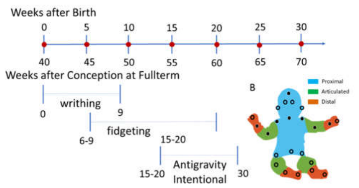
Figure 2.
Dyadic sensors location. (A) Advanced light weight APDM Opal samples at 128Hz with battery life of 12 hours and in-sensor storage up to 8Gigabytes. (B) Elastic straps enable affixing the sensors to different body locations. (C) Schematics from APDM manual of suggested body locations to affix the sensors. (D) Actual locations used in the study using 6 sensors on each person, the child and the practitioner. Red circles indicate the location. Insets show the straps used in the study to avoid interference with the exercises.
Figure 2.
Dyadic sensors location. (A) Advanced light weight APDM Opal samples at 128Hz with battery life of 12 hours and in-sensor storage up to 8Gigabytes. (B) Elastic straps enable affixing the sensors to different body locations. (C) Schematics from APDM manual of suggested body locations to affix the sensors. (D) Actual locations used in the study using 6 sensors on each person, the child and the practitioner. Red circles indicate the location. Insets show the straps used in the study to avoid interference with the exercises.
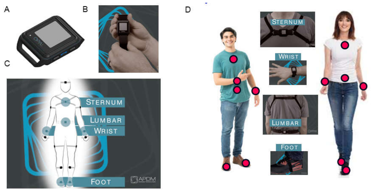
Figure 3.
Experimental Protocol. (A) Room at the school where experiment took place. Padded tables and floor mats were used for different exercises, creating a safe environment for the child. Chairs to the left-hand side were used for interviews before each session. A Cannon camera on tripods and 2 Go Pro cameras registered the 25 sessions. (B) Sensors’ station and annotator registering all behavioral states. Setting up sensors with different colored sports tapes helped maintain consistency of sensor location. Annotations highlighted any remarkable behavioral landmarks throughout the sessions. (C) Representative performance of the standardized tasks performed pre- and post- intervention. The resting task, where the child is asked to remain still and the practitioner performs the task in tandem with the child. (D) During the pointing task, the child is asked to point to visual targets located at a comfortable reaching distance. This task was also performed in tandem with the practitioners (two different practitioners are shown here for the AM and the PM sessions). (E) The sit-to-stand task performed in tandem with the practitioner during the AM and PM sessions respectively.
Figure 3.
Experimental Protocol. (A) Room at the school where experiment took place. Padded tables and floor mats were used for different exercises, creating a safe environment for the child. Chairs to the left-hand side were used for interviews before each session. A Cannon camera on tripods and 2 Go Pro cameras registered the 25 sessions. (B) Sensors’ station and annotator registering all behavioral states. Setting up sensors with different colored sports tapes helped maintain consistency of sensor location. Annotations highlighted any remarkable behavioral landmarks throughout the sessions. (C) Representative performance of the standardized tasks performed pre- and post- intervention. The resting task, where the child is asked to remain still and the practitioner performs the task in tandem with the child. (D) During the pointing task, the child is asked to point to visual targets located at a comfortable reaching distance. This task was also performed in tandem with the practitioners (two different practitioners are shown here for the AM and the PM sessions). (E) The sit-to-stand task performed in tandem with the practitioner during the AM and PM sessions respectively.
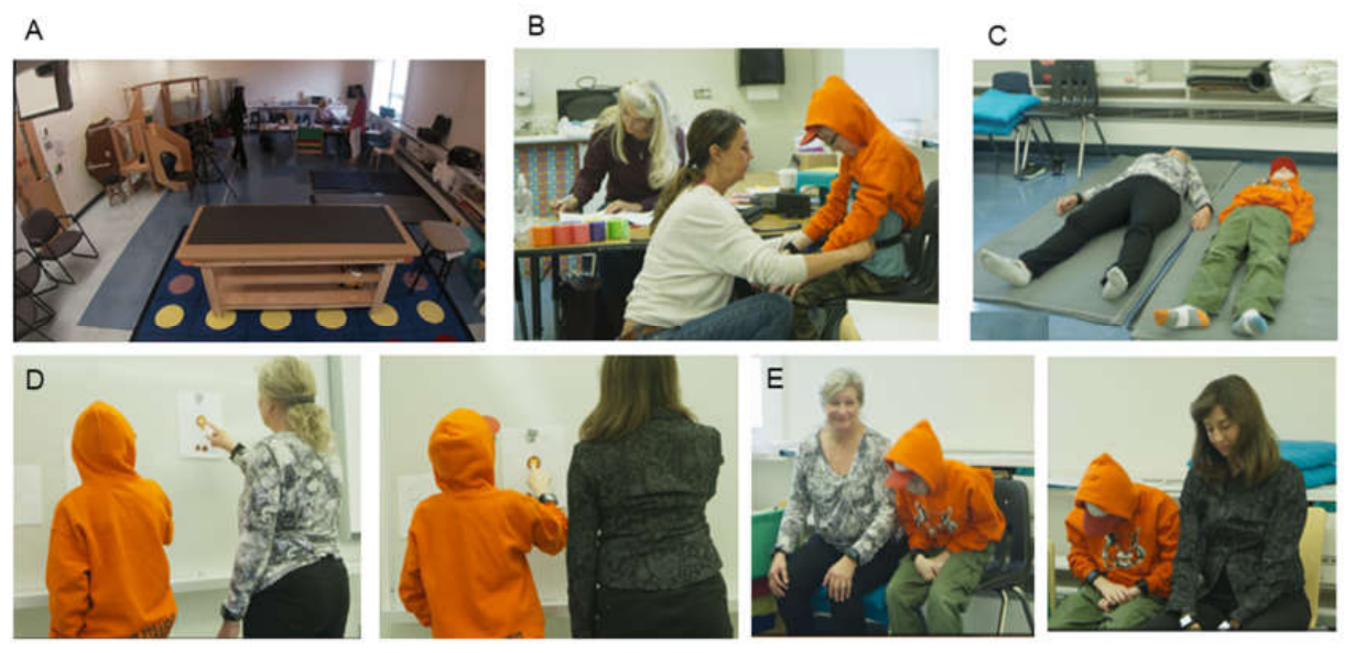
Figure 4.
Representative routines of the intervention aimed at increasing awareness of the body from head to toe as the practitioner exchanges subtle and slow motions with the child building awareness of self-generated movements.
Figure 4.
Representative routines of the intervention aimed at increasing awareness of the body from head to toe as the practitioner exchanges subtle and slow motions with the child building awareness of self-generated movements.
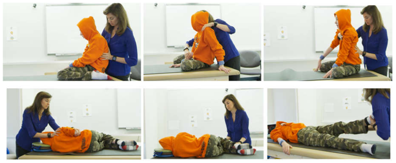
Figure 5.
Analytical pipeline. (A) Raw linear acceleration at resting state from sensors of the upper body pre- and post-intervention. Black dots denote peaks (where the slope of the acceleration curve transitions from positive to negative). Green line denotes the empirically estimated Gamma mean from (B) showing the histogram of the peaks in (A) and the best fitting Gamma PDF (in a maximum likelihood estimation sense). (C) Absolute deviations from the empirical Gamma mean. (D) Micro-movements spikes derived from applying Equation 2 to the absolute mean deviations in (C) to scale out allometric effects due to disparate anatomical lengths. Zero values are at mean acceleration level. (E) Gamma plane representation of the MMS distribution parameter values pre- and post-intervention. The estimated distributions are represented by points (shape, scale) on the Gamma parameter plane, with 95% confidence intervals. (F) The corresponding estimated probability density functions for pre- and post-intervention resting state. (G) Estimated Gamma moments parameter space representing the mean along the x-axis, the variance along the y-axis, the skewness along the z-axis and kurtosis proportional to the size of the marker (smaller is lower kurtosis). (H) The projection of the points on the Г-scale which is the noise to signal ratio. Notice there is a reduction in the NSR post intervention and an increase in the skewness.
Figure 5.
Analytical pipeline. (A) Raw linear acceleration at resting state from sensors of the upper body pre- and post-intervention. Black dots denote peaks (where the slope of the acceleration curve transitions from positive to negative). Green line denotes the empirically estimated Gamma mean from (B) showing the histogram of the peaks in (A) and the best fitting Gamma PDF (in a maximum likelihood estimation sense). (C) Absolute deviations from the empirical Gamma mean. (D) Micro-movements spikes derived from applying Equation 2 to the absolute mean deviations in (C) to scale out allometric effects due to disparate anatomical lengths. Zero values are at mean acceleration level. (E) Gamma plane representation of the MMS distribution parameter values pre- and post-intervention. The estimated distributions are represented by points (shape, scale) on the Gamma parameter plane, with 95% confidence intervals. (F) The corresponding estimated probability density functions for pre- and post-intervention resting state. (G) Estimated Gamma moments parameter space representing the mean along the x-axis, the variance along the y-axis, the skewness along the z-axis and kurtosis proportional to the size of the marker (smaller is lower kurtosis). (H) The projection of the points on the Г-scale which is the noise to signal ratio. Notice there is a reduction in the NSR post intervention and an increase in the skewness.
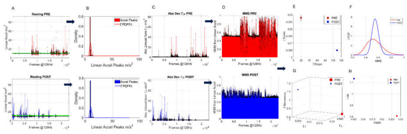
Figure 6.
Transfer entropy and network connectivity analysis of the dyad. (A) Representative matrix with color coded pairwise transfer entropy values for each of the body parts of the practitioner (rows 1-6) and the student (rows 7-12) for one session. Row-wise indicates that higher values lead. In this case, knowing information about the student’s past activity lowers the uncertainty of predicting the practitioner’s future activity, particularly at the sacrum and left ankle. (B) MMS from the right wrist of the student and practitioner and output from power spectral analysis. (C) Values of coherence estimates (0-1) as a function of frequency (0-64 in 128Hz), obtained between representative MMS in B for 1 minute of the session, and corresponding cross-spectrum phase (deg) at the bottom graph. For example, data tip labels indicate maximum value of 0.79 corresponding to cross-spectrum phase of 49.37 at frequency 24.93. (D) Resulting pairwise matrix of cross-coherence values. (E) These are coherence values above a 0.75 threshold to isolate the higher cross-coherence peaks and examine the corresponding cross-spectrum phase values depicted in matrix form in (F) across corresponding frequencies in (G). (H-K) Example of network connectivity metrics obtained across all sensors for the session time, 40min in this case including 5min pre- and 5min post-standard tasks. (L) Sample grouping of node (sensor on body part) participation in each module identified in (H) across the session. (M) Sample representation of network state (one frame of a movie spanning the number of minutes of the session) to appreciate the modules through the colors of the circles, the connectivity (in and out degree counting the number of edges through the node, proportional to the size of the circle) within the body and across the two agents of the dyad. Student is on the right and practitioner on the left. For example, this frame depicts two modules sharing the connectivity of the 2 sternum nodes, the left wrist and left ankle of the practitioner and the two ankles of the student (in red). The other module (green) shares the two lumbar nodes with the right wrist and left ankle of the practitioner and the two wrists of the student (in green). The size of the circles gives the total degree (in and out edges) while the black circle is the betweenness centrality value of the node for that minute-frame of the network connectivity state.
Figure 6.
Transfer entropy and network connectivity analysis of the dyad. (A) Representative matrix with color coded pairwise transfer entropy values for each of the body parts of the practitioner (rows 1-6) and the student (rows 7-12) for one session. Row-wise indicates that higher values lead. In this case, knowing information about the student’s past activity lowers the uncertainty of predicting the practitioner’s future activity, particularly at the sacrum and left ankle. (B) MMS from the right wrist of the student and practitioner and output from power spectral analysis. (C) Values of coherence estimates (0-1) as a function of frequency (0-64 in 128Hz), obtained between representative MMS in B for 1 minute of the session, and corresponding cross-spectrum phase (deg) at the bottom graph. For example, data tip labels indicate maximum value of 0.79 corresponding to cross-spectrum phase of 49.37 at frequency 24.93. (D) Resulting pairwise matrix of cross-coherence values. (E) These are coherence values above a 0.75 threshold to isolate the higher cross-coherence peaks and examine the corresponding cross-spectrum phase values depicted in matrix form in (F) across corresponding frequencies in (G). (H-K) Example of network connectivity metrics obtained across all sensors for the session time, 40min in this case including 5min pre- and 5min post-standard tasks. (L) Sample grouping of node (sensor on body part) participation in each module identified in (H) across the session. (M) Sample representation of network state (one frame of a movie spanning the number of minutes of the session) to appreciate the modules through the colors of the circles, the connectivity (in and out degree counting the number of edges through the node, proportional to the size of the circle) within the body and across the two agents of the dyad. Student is on the right and practitioner on the left. For example, this frame depicts two modules sharing the connectivity of the 2 sternum nodes, the left wrist and left ankle of the practitioner and the two ankles of the student (in red). The other module (green) shares the two lumbar nodes with the right wrist and left ankle of the practitioner and the two wrists of the student (in green). The size of the circles gives the total degree (in and out edges) while the black circle is the betweenness centrality value of the node for that minute-frame of the network connectivity state.
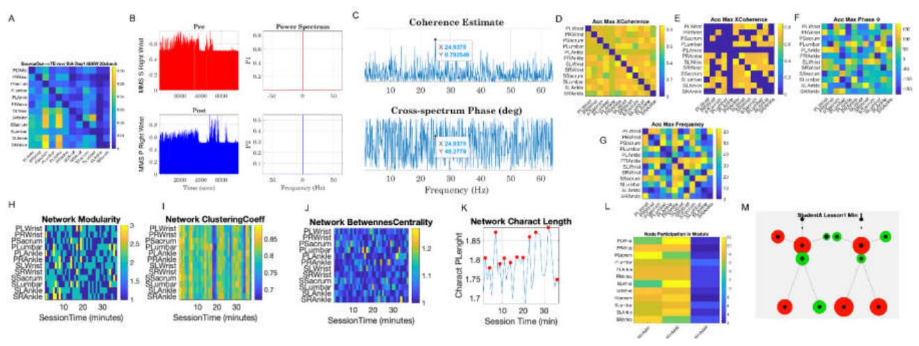
Figure 7.
Significant reduction in Г-NSR (Г-variance/Г-mean) across all three standard tasks when comparing pre- and post-intervention values of the Г-NSR across the body, as captured by the linear acceleration MMS and the empirically estimated continuous Г-family of PDFs best characterizing the motions of the student and the practitioner.
Figure 7.
Significant reduction in Г-NSR (Г-variance/Г-mean) across all three standard tasks when comparing pre- and post-intervention values of the Г-NSR across the body, as captured by the linear acceleration MMS and the empirically estimated continuous Г-family of PDFs best characterizing the motions of the student and the practitioner.
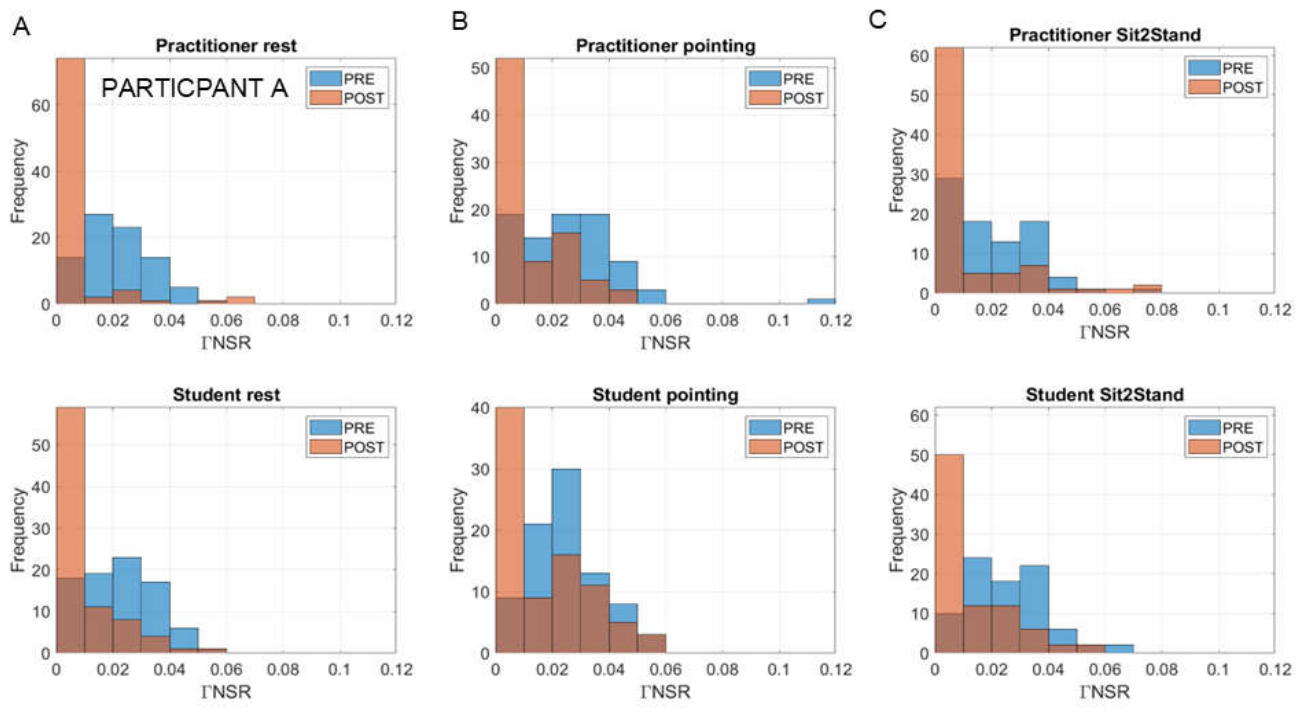
Figure 8.
Shifts in the Г-shape and Г-scale (NSR) parameters across the body for the student and practitioner pre- and post-intervention for the resting task. (A) Inverse linear relation between the Г-scale (NSR) and Г-shape on the log-log Г-parameter plane. As the noise drops, the shape of the distribution tends to the Gaussian range of the continuous Г-family. Marker size is proportional to session date, with smaller markers being earlier in the sessions than larger markers. (B) Statistically significant shifts according to the non-parametric ANOVA (Kruskal Wallis test) and tables reporting the p-values. (C) Corresponding shifts in the Г-moments (Г-mean and Г-variance) post minus pre reveal concentration of the scatter in the negative quadrant signaling that mostly, across sessions, post Г-scale (NSR) < pre Г-scale (NSR), with the MMS Г-variance explaining the drop in Г-NSR at rest.
Figure 8.
Shifts in the Г-shape and Г-scale (NSR) parameters across the body for the student and practitioner pre- and post-intervention for the resting task. (A) Inverse linear relation between the Г-scale (NSR) and Г-shape on the log-log Г-parameter plane. As the noise drops, the shape of the distribution tends to the Gaussian range of the continuous Г-family. Marker size is proportional to session date, with smaller markers being earlier in the sessions than larger markers. (B) Statistically significant shifts according to the non-parametric ANOVA (Kruskal Wallis test) and tables reporting the p-values. (C) Corresponding shifts in the Г-moments (Г-mean and Г-variance) post minus pre reveal concentration of the scatter in the negative quadrant signaling that mostly, across sessions, post Г-scale (NSR) < pre Г-scale (NSR), with the MMS Г-variance explaining the drop in Г-NSR at rest.
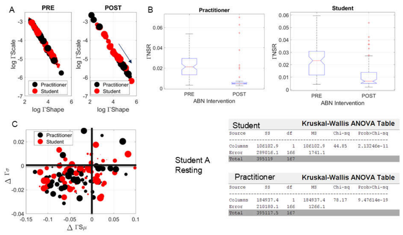
Figure 9.
Upper body’s rapid and highly significant shift in Г-NSR and Г-PDF skewness from morning (top) to afternoon (bottom) sessions in Day 1 of the intervention (linear acceleration). (A) Minute-by-minute signatures of the session for the left wrist of student (red) and practitioner (blue). Time represented proportional to the size of the marker, whereby earlier minutes are smaller size markers, and later minutes are larger size markers. Projection parameter-plane from the Г moments localize points representing them as (Г-NSR, Г-Skewness). (B) Unfolding the evolution of the session minute-by-minute. Second session in the afternoon on the bottom panel shows the shifting of the Г-NSR trending to an alignment of the student’s signatures onto the practitioner’s signatures around minute 20. (C-F) Similar as in A-B for the lumbar and right wrist sensors.
Figure 9.
Upper body’s rapid and highly significant shift in Г-NSR and Г-PDF skewness from morning (top) to afternoon (bottom) sessions in Day 1 of the intervention (linear acceleration). (A) Minute-by-minute signatures of the session for the left wrist of student (red) and practitioner (blue). Time represented proportional to the size of the marker, whereby earlier minutes are smaller size markers, and later minutes are larger size markers. Projection parameter-plane from the Г moments localize points representing them as (Г-NSR, Г-Skewness). (B) Unfolding the evolution of the session minute-by-minute. Second session in the afternoon on the bottom panel shows the shifting of the Г-NSR trending to an alignment of the student’s signatures onto the practitioner’s signatures around minute 20. (C-F) Similar as in A-B for the lumbar and right wrist sensors.
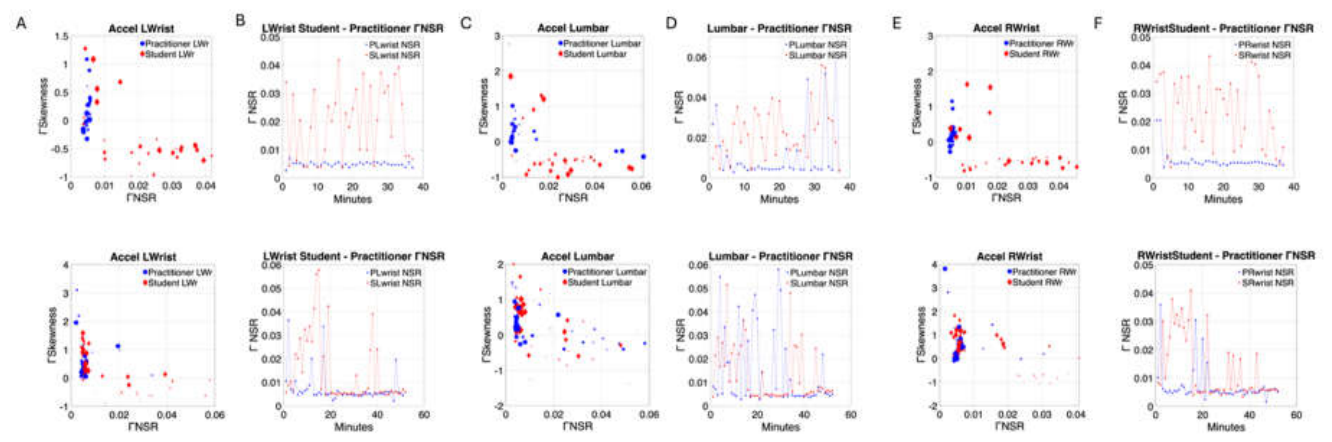
Figure 10.
Lower body’s rapid and highly significant shift in Г-NSR and Г-PDF skewness from morning (top) to afternoon (bottom) sessions in Day 1 of the intervention (linear acceleration). (A) Minute-by-minute signatures of the session for the left ankle of student (red) and practitioner (blue). As in Figure 9, time is represented proportional to the size of the marker, whereby earlier minutes are smaller size markers, and later minutes are larger size markers. Projection parameter-plane from the Г moments localize points representing them as (Г-NSR, Г-Skewness). (B) Unfolding the evolution of the session minute-by-minute. Second session in the afternoon on the bottom panel shows the shifting of the Г-NSR trending to an alignment of the student’s signatures towards the practitioner’s signatures. (C-F) Similar as in A-B for the sacrum and right ankle sensors.
Figure 10.
Lower body’s rapid and highly significant shift in Г-NSR and Г-PDF skewness from morning (top) to afternoon (bottom) sessions in Day 1 of the intervention (linear acceleration). (A) Minute-by-minute signatures of the session for the left ankle of student (red) and practitioner (blue). As in Figure 9, time is represented proportional to the size of the marker, whereby earlier minutes are smaller size markers, and later minutes are larger size markers. Projection parameter-plane from the Г moments localize points representing them as (Г-NSR, Г-Skewness). (B) Unfolding the evolution of the session minute-by-minute. Second session in the afternoon on the bottom panel shows the shifting of the Г-NSR trending to an alignment of the student’s signatures towards the practitioner’s signatures. (C-F) Similar as in A-B for the sacrum and right ankle sensors.
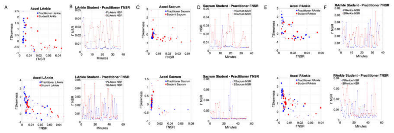
Figure 11.
Rapid shifts in ГNSR obtained from the micromovements derived from the fluctuations in bodily acceleration between morning and afternoon during the intensive sessions. (A) Student A shows in each panel the upper body distal (right and left wrists), the lower body distal (right and left ankle) and the proximal segments (lumbar and sacrum) where the sensors were located. First day of intensive session shows the dramatic chance in ГNSR. (B) Student C with similar layout as panel A. (C) Student E with similar layout as panels A and B during transition from lesson 2 to lesson 3.
Figure 11.
Rapid shifts in ГNSR obtained from the micromovements derived from the fluctuations in bodily acceleration between morning and afternoon during the intensive sessions. (A) Student A shows in each panel the upper body distal (right and left wrists), the lower body distal (right and left ankle) and the proximal segments (lumbar and sacrum) where the sensors were located. First day of intensive session shows the dramatic chance in ГNSR. (B) Student C with similar layout as panel A. (C) Student E with similar layout as panels A and B during transition from lesson 2 to lesson 3.
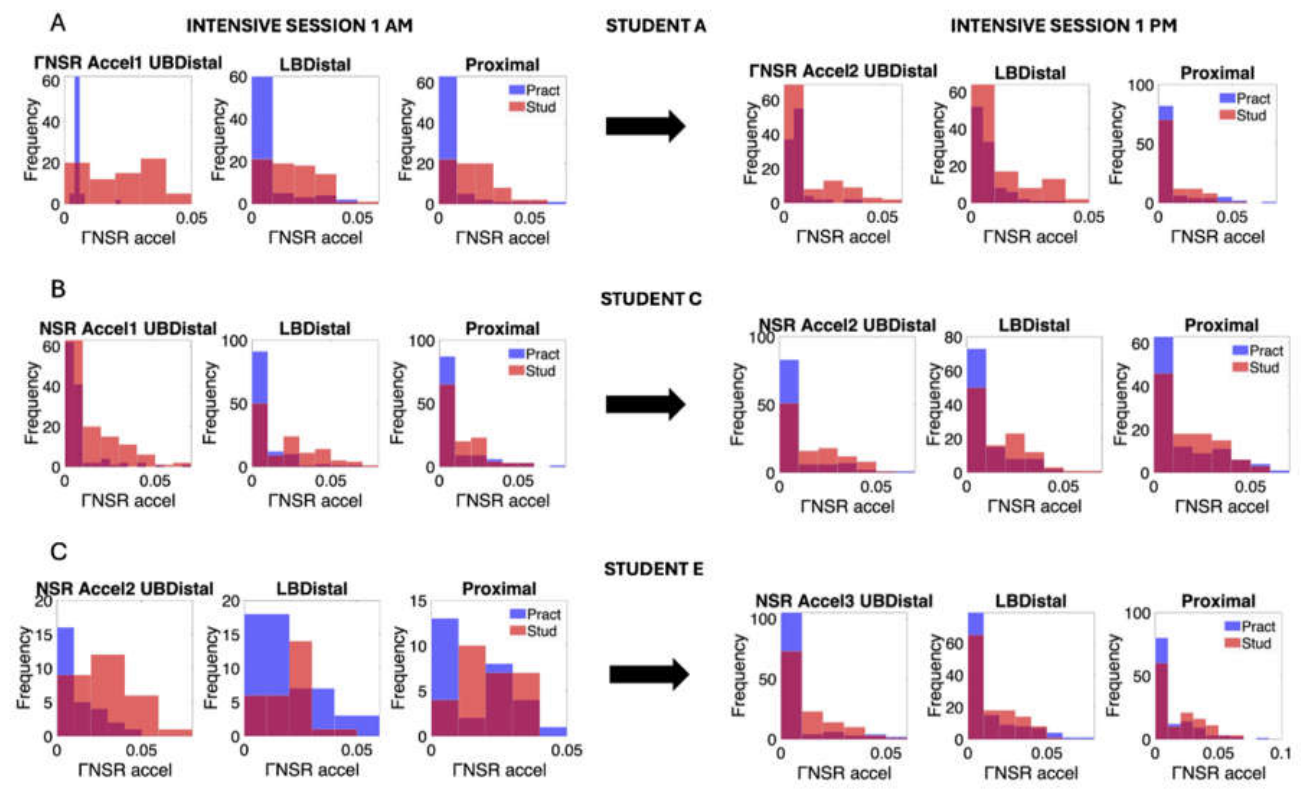
Figure 12.
Alignment of the ГNSR values across body segments and sessions for the practitioner and student. (A) Student A. (B) Comparison of p-values using the Wilcoxon rank sum test between the practitioner and student patterns for each body segment (red proximal, blue upper body distal and green lower body distal). Peaks above dashed line denote significance at the .05 level while those above the full line denote significance above .01 level. Points below the lines are not statistically significant suggesting more similar median values of the ГNSR between the practitioner and child for that session. (C)–(D) Same as in (A)–(B) for the participant C. (E)–(F) for participant E.
Figure 12.
Alignment of the ГNSR values across body segments and sessions for the practitioner and student. (A) Student A. (B) Comparison of p-values using the Wilcoxon rank sum test between the practitioner and student patterns for each body segment (red proximal, blue upper body distal and green lower body distal). Peaks above dashed line denote significance at the .05 level while those above the full line denote significance above .01 level. Points below the lines are not statistically significant suggesting more similar median values of the ГNSR between the practitioner and child for that session. (C)–(D) Same as in (A)–(B) for the participant C. (E)–(F) for participant E.
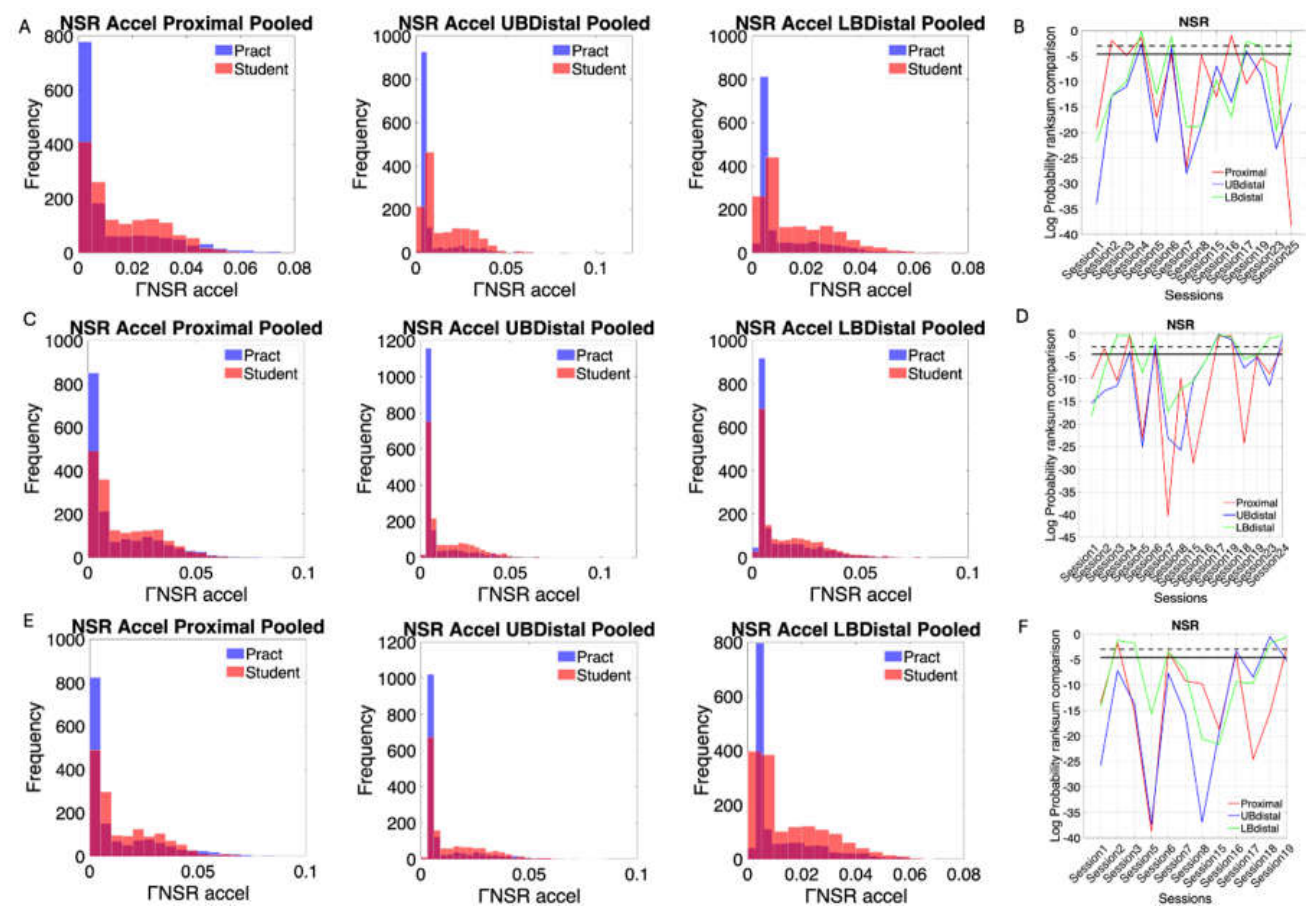
Figure 13.
Network connectivity analysis of global and local networks reveals similar patterns in the joint dyadic network and the individual network of each agent. (A) Student A modularity of the global network comprised of 12 nodes in the intensive and sporadic sections reveal 2-3 modules which are also present in the individual 6-node network of each agent. (B) Betweenness centrality metric also shows similar ranges between the global and local networks with appreciable differences in distribution for the global network between the intensive and the sporadic sessions. Inset panel shows the overlapping in global patterns of the characteristic path length. (D-E-F) Student C patterns shown in the same format as Student A, reveal similar trends between the global and the local networks. (G-H-I) Student E patterns are consistent with those of Students A and C.
Figure 13.
Network connectivity analysis of global and local networks reveals similar patterns in the joint dyadic network and the individual network of each agent. (A) Student A modularity of the global network comprised of 12 nodes in the intensive and sporadic sections reveal 2-3 modules which are also present in the individual 6-node network of each agent. (B) Betweenness centrality metric also shows similar ranges between the global and local networks with appreciable differences in distribution for the global network between the intensive and the sporadic sessions. Inset panel shows the overlapping in global patterns of the characteristic path length. (D-E-F) Student C patterns shown in the same format as Student A, reveal similar trends between the global and the local networks. (G-H-I) Student E patterns are consistent with those of Students A and C.
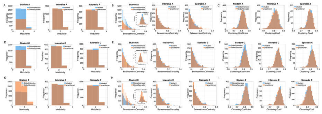
Figure 14.
The lead-lag dance between the student and the practitioner captured by the measurement of transfer entropy (TE) of selected sessions. (A) Student A. Pairwise computation of TE across the 12 nodes of the practitioner and the student. The matrix entry is the TE value from the two streams of micro-movements derived from the two body parts. The TE reads along the rows as the row entry leading the column entry. In Day 1 we appreciate the student’s lead over the practitioner’s upper body limbs, lumbar and sacrum regions. In Day 2 the lead patterns continue stronger for the student over the practitioner, with more engagement of the practitioner’s body parts, specially involving the lumbar and sacrum regions leading over her own other body parts. Day 3 strengthens student’s lead pattern which shifts in day 6 to the lower limbs (left and right ankles with the practitioner leading the student and the student himself sharing this dance by leading his lower limbs. By Day 16, the pattern shifts to the upper limbs (right and left wrists) and to a lower degree, the right and left ankles. (B) Student C has a more complex pattern of TE but also shares a dance of leading and lagging the practitioner. (C) Student E shows initial lead by the student that evolves over the sessions to the practitioner’s lead. These dynamic patterns demonstrate the complexity of the sessions.
Figure 14.
The lead-lag dance between the student and the practitioner captured by the measurement of transfer entropy (TE) of selected sessions. (A) Student A. Pairwise computation of TE across the 12 nodes of the practitioner and the student. The matrix entry is the TE value from the two streams of micro-movements derived from the two body parts. The TE reads along the rows as the row entry leading the column entry. In Day 1 we appreciate the student’s lead over the practitioner’s upper body limbs, lumbar and sacrum regions. In Day 2 the lead patterns continue stronger for the student over the practitioner, with more engagement of the practitioner’s body parts, specially involving the lumbar and sacrum regions leading over her own other body parts. Day 3 strengthens student’s lead pattern which shifts in day 6 to the lower limbs (left and right ankles with the practitioner leading the student and the student himself sharing this dance by leading his lower limbs. By Day 16, the pattern shifts to the upper limbs (right and left wrists) and to a lower degree, the right and left ankles. (B) Student C has a more complex pattern of TE but also shares a dance of leading and lagging the practitioner. (C) Student E shows initial lead by the student that evolves over the sessions to the practitioner’s lead. These dynamic patterns demonstrate the complexity of the sessions.
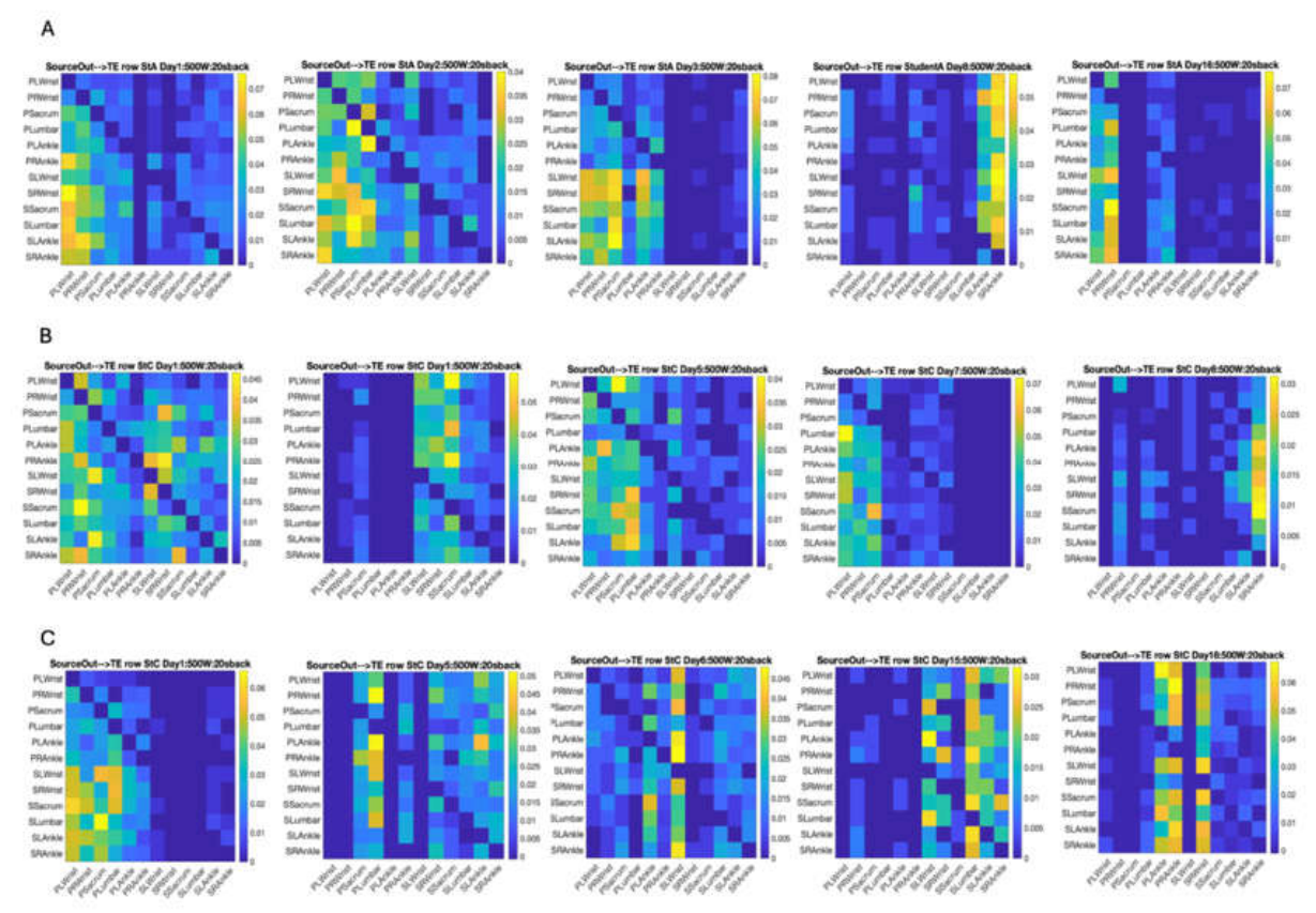
Figure 15.
Intensive vs. Tapered off sessions measuring the interplay of agency between the student and practitioner. (A) Student A, Proximal sensor locations (lumbar and sacrum) for intensive and sporadic. (B) Student A, upper limbs (right and left wrists). (C) Student A, lower limbs (right and left ankles). (D-F) Same as in A-C for student C showing a far more complex and variable pattern. (G-I) Same as above for student E.
Figure 15.
Intensive vs. Tapered off sessions measuring the interplay of agency between the student and practitioner. (A) Student A, Proximal sensor locations (lumbar and sacrum) for intensive and sporadic. (B) Student A, upper limbs (right and left wrists). (C) Student A, lower limbs (right and left ankles). (D-F) Same as in A-C for student C showing a far more complex and variable pattern. (G-I) Same as above for student E.
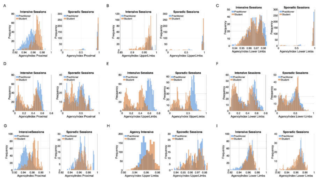

Table 1.
Pre- and post-intervention comparison of Г-NSR levels across pooled data from all sensors (student vs. practitioner) and broken down by body region.
Table 1.
Pre- and post-intervention comparison of Г-NSR levels across pooled data from all sensors (student vs. practitioner) and broken down by body region.
| Dyad All sensors | Kruskal Wallis Test Chi-sq, p>Chi-sq |
|---|---|
| Student A | 641.02, 2.005 e-141 |
| Student C | 409.83, 3.991 e-91 |
| Student E | 310.54, 1.668 e-69 |
| Upper body Distal | |
| Student A | 313.52, 3.743 e-70 |
| Student C | 191.07, 1.856 e-43 |
| Student E | 147.93, 4.912 e-34 |
| Lower body Distal | |
| Student A | 190.75, 2.183 e-43 |
| Student C | 65.40, 6.112 e-16 |
| Student E | 42.78, 6.133 e-11 |
| Proximal | |
| Student A | 180.07, 4.687 e-41 |
| Student C | 1.64.0, 1.512 e-37 |
| Student E | 145.18, 1.959 e-33 |
Disclaimer/Publisher’s Note: The statements, opinions and data contained in all publications are solely those of the individual author(s) and contributor(s) and not of MDPI and/or the editor(s). MDPI and/or the editor(s) disclaim responsibility for any injury to people or property resulting from any ideas, methods, instructions or products referred to in the content. |
© 2026 by the authors. Licensee MDPI, Basel, Switzerland. This article is an open access article distributed under the terms and conditions of the Creative Commons Attribution (CC BY) license (http://creativecommons.org/licenses/by/4.0/).
Copyright: This open access article is published under a Creative Commons CC BY 4.0 license, which permit the free download, distribution, and reuse, provided that the author and preprint are cited in any reuse.