

Submitted:
23 October 2026
Posted:
26 October 2026
You are already at the latest version
Abstract
Credit allocation is usually left to a threshold rule applied to machine-learning estimates of default risk, and the stability of the explanations that justify it is rarely measured and never required. We formulate credit allocation as a stochastic combinatorial problem that minimises the conditional value-at-risk of portfolio loss subject to a return floor, a minimum ticket, an origination cost and a cap on the exposure-weighted instability of the Shapley attributions of the funded book. We solve it with a two-level simheuristic: a variable neighbourhood search over which applicants to fund, started from a rounded linear relaxation, and a simulation-driven cutting-plane method that optimises the amounts to a certified tolerance. On Polish bankruptcy data, with a Taiwanese cardholder dataset as control, the tail criterion gives up 9.2 per cent of expected profit out of sample and multiplies the profit retained in the worst 5 per cent of scenarios by 4.6. Stable explanations are costly on the primary data and free on the control. The exact solver proves optimality up to 75 applicants; at 100, where it proves none within an hour, the simheuristic matches its best incumbent in 45 seconds, within a certified 2.6 per cent.
Keywords:
simheuristics
; conditional value-at-risk
; explainable artificial intelligence
; SHAP stability
; credit allocation
; variable neighbourhood search
; mixed-integer programming
; sample average approximation
1. Introduction
A lender with a finite budget must decide which firms to fund and how much to commit to each, knowing that it cannot meet every request. The decision is taken under uncertainty — a borrower may default, and the loss it causes depends on how much was committed to it — and it is, at its core, a constrained allocation problem rather than a pure prediction problem. The problem is most acute where credit is scarce, as it is for small and medium-sized firms in emerging economies, which motivate this line of work. The present study, however, addresses firm-level credit allocation in general: the data on which it is validated do not classify firms by size, and its evidence is not specific to smaller firms (Section 7).
The literature has advanced considerably on the prediction side. Machine learning has become the dominant paradigm for credit-risk assessment and financial-distress forecasting, with ensemble methods consistently outperforming logistic regression and discriminant models across a range of national settings [1,2,3,4]. Gains are real but uneven, and evaluation practice has not converged: studies differ in whether they report the area under the curve, the Kolmogorov–Smirnov statistic, F1 or accuracy alone, and comparatively few report the full suite that credit-risk practice arguably requires [5,6].
A parallel stream has established explainable artificial intelligence as a governance requirement rather than a technical refinement. Shapley additive explanations have become the de facto standard for post-hoc attribution in credit applications, frequently triangulated with local surrogates and partial dependence [7,8,9]. The motivation is largely regulatory: a credit decision that cannot be explained to the applicant, the supervisor or a court is increasingly untenable, whatever its accuracy. Yet explainability in this literature is applied almost exclusively as a diagnostic layer, after a model has been trained and before a decision is taken by some separate mechanism. It informs the analyst; it does not enter the decision.
This is the discontinuity that motivates the present study. Prediction and decision are treated as separate problems. A model estimates a probability of default, and the allocation that follows is typically resolved by a threshold rule — approve below a cut-off, decline above it — or by a policy that the published work does not formalise. Where optimisation does appear in the credit literature, it is directed at the model rather than at the decision: an independent review finds that metaheuristics and mathematical programming are used overwhelmingly for feature selection, hyper-parameter search and threshold tuning [10], not for allocating a constrained budget across a portfolio of counterparties whose defaults are uncertain.
Simheuristics offer a principled way to close that discontinuity. By embedding Monte Carlo simulation inside a metaheuristic search, they address stochastic combinatorial optimisation problems whose objective cannot be evaluated in closed form and whose solution space is too large for exact methods to be practical [11,12,13]. The structure of the credit allocation problem — a combinatorial choice of which counterparties to fund, and how much, whose payoff depends on random events realised after the decision — matches that class closely. Financial applications of this machinery exist, and Section 2.6 and Section 2.8 identify several; what none of them adopts is a risk-averse criterion together with a scalable search, and none couples an explainable risk signal to the allocation as a constraint.
Three observations therefore define the gap this paper addresses. First, predictive accuracy and decision optimisation are pursued in isolation, and the translation of a risk forecast into an allocation is left unformalised. Second, the stability of explanations has begun to be measured [14] but has nowhere been made binding on the decision that the explanation is meant to justify. Third, evaluation practice remains inconsistent and, in several published cases, methodologically fragile — one reviewed study reports an area under the curve of 1.0 on a sample whose labels are derived from the same quantities used as predictors [15] — which argues for benchmarking against a wider and more rigorously validated suite.
Accordingly, this paper makes the following contributions, which are algorithmic and methodological in nature; the financial setting is the domain of application, not the object of study.
- We formulate credit allocation under default risk as a single-period stochastic combinatorial optimisation problem that minimises the conditional value-at-risk of portfolio loss, written in the Rockafellar–Uryasev form [16,17], subject to a floor on expected return. A minimum ticket and a fixed origination cost give the activation decision content and make the sample-average approximation a mixed-integer programme, and we measure when that structure binds: on the base instance of 25 applicants the linear relaxation is tight and the activation parameters change the value but not the decision, whereas at 100 applicants the relaxation funds names partially and below the minimum ticket.
- We propose a two-level simheuristic in which a calibrated machine-learning model supplies the default probabilities that parameterise the simulation, a variable neighbourhood search, started from a rounded linear relaxation, chooses which counterparties to fund, and a simulation-driven cutting-plane method optimises the amounts on each candidate support to a certified tolerance. Prediction thereby parameterises optimisation rather than substituting for it.
- We introduce an explanation-stability constraint that caps the exposure-weighted instability of the Shapley attributions underlying the risk estimates of the funded book, under bounded perturbation of the inputs. Explainability becomes a restriction on the feasible set rather than a commentary on a decision already taken; a stricter per-counterparty filter is reported as a robustness variant, and its cost is measured.
- We benchmark the framework against the exact mixed-integer solution of the sample-average approximation, a deterministic formulation, a threshold policy that ranks applicants by expected net return, a risk-neutral ablation and the sample average approximation method at the same scenario count, and we evaluate every plan out of sample on thirty independent scenario samples with common random numbers, so that each comparison carries a paired confidence interval. Every exact result is reported as a proven optimum or as an incumbent with its gap.
Three findings stand out. The tail criterion buys a large reduction in tail risk for a moderate sacrifice of expected profit on both datasets, and threshold rules are dominated even when they rank by expected return. The cost of requiring stable explanations depends on the data: it is material on the primary dataset and nil on the control, and imposing stability applicant by applicant rather than on the portfolio roughly doubles it. And the simheuristic reaches the proven optimum in every run on the base instance, in a small fraction of the time, and on independent instances of 50 and 75 applicants stops within 0.22 per cent of an optimum the exact solver still proves; at 100 applicants, where the linear relaxation is not tight and the exact solver fails to prove optimality within an hour, it matches the solver’s incumbent in 45 seconds, with a certified gap to the optimum of at most 2.6 per cent.
The remainder of the paper is organised as follows. Section 2 reviews the related work. Section 3 states the problem and the formal model. Section 4 describes the solution framework. Section 3 to Section 5 together play the role of a materials-and-methods section: Section 5 sets out the experimental design, datasets, validation protocol and computational environment, Section 6 reports the results, Section 7 discusses implications and limitations, and Section 8 concludes.
2. Related Work
This section reviews two bodies of literature that have developed largely in parallel and that the present study brings together. The first concerns data analytics, machine learning and explainable artificial intelligence applied to credit risk and financial distress, principally in small and medium-sized enterprises. The second concerns metaheuristic and simheuristic optimisation under uncertainty, and in particular the treatment of risk aversion through the conditional value-at-risk criterion. The review closes by identifying the gap that motivates our contribution: the absence of any treatment of explanation stability as a constraint on the decision that the explanation is meant to justify.
The corpus was assembled through two structured searches. The first, covering the analytics and machine-learning literature, was executed in Scopus on 3 September 2026 over titles, abstracts and keywords, restricted to journal articles published between 2022 and 2026, and combining terms for learning methods, explainability, credit and liquidity problems, and SME or emerging-market settings; it retrieved 117 records, of which 116 were unique, and 25 were retained for detailed extraction. The second search covered stochastic and metaheuristic optimisation and yielded 25 references spanning 2000 to 2026. A further seven methodological references, on sample average approximation, cutting-plane solution, Shapley attribution and probability calibration, were added as the formulation and the solution method took shape; they are cited in Section 3 to Section 5 rather than in this review. The consolidated bibliography therefore comprises 57 entries. One methodological caveat applies to the first corpus and is stated rather than left implicit: that every retained record falls within 2022–2026 is a consequence of the publication-year filter, not evidence that the field has renewed within that window.
2.1. Machine Learning for Credit Risk and Financial Distress Prediction
Ensemble learning has become the dominant paradigm for credit risk assessment and distress prediction in SMEs. Across markets and sample designs, random forests, gradient boosting, XGBoost and their variants outperform logistic regression and Altman-style discriminant models with striking regularity [1,2,3], and random forest is the single most frequently reported best performer. The consistency of this finding across heterogeneous settings is itself informative: it suggests that the marginal return to further architectural refinement of the classifier is diminishing, and that the binding constraints on practical usefulness now lie elsewhere.
The distress-prediction tradition has been extended across a wide range of emerging economies, including Thailand [20], India [21], Indonesia [22], Albania [1] and Vietnam [2,23], and has broadened the feature space well beyond accounting ratios. Intellectual capital materially improves discriminatory power in large SME samples [3]; behavioural and transactional data fused with static firm characteristics improve credit-risk prediction in supply-chain finance [4]; and supply-chain indicators combined with synthetic augmentation have been used against the severe class imbalance typical of default data [24].
Class imbalance is the methodological obstacle that recurs most often, and the responses are varied: imbalance-aware sub-sampling with rule extraction [25], oversampling and bagging within multi-stage ensembles [5], generative tabular augmentation [24], and explicit comparison of sampling strategies against a common classifier set [26]. A parallel line develops SME-specific architectures that combine heuristic or evolutionary feature selection with stacked ensembles and Bayesian meta-learners [27,28], which is where the predictive literature begins to borrow from the optimisation literature of Section 2.5 and Section 2.6.
Evaluation practice, by contrast, has not converged. Reported metrics range from accuracy alone to full suites including the area under the curve, F1 and the Kolmogorov–Smirnov statistic, with only a minority reporting the complete set [5,6]. More consequential for the present work is what is almost never reported: probability calibration. Most studies evaluate discrimination and stop there. Yet whenever an estimated default probability enters a stochastic optimisation model as the parameter of a Bernoulli event, as it does here, it is calibration rather than discrimination that determines whether the resulting decision is sound: a model that ranks perfectly but is systematically overconfident produces scenario sets that misstate the loss distribution, and a risk measure computed on the wrong support. Only a small number of studies address calibration explicitly [20,23], and Yang and Xiao [5] are unusual in reporting a Brier score. At the opposite extreme, Akhmetova et al. [29] report an area under the curve of 0.371 on a chronologically ordered test set — below random assignment — while presenting the framework as interpretable, which shows that interpretability and discrimination are not substitutes. A further distinction matters and is absent from the reviewed corpus: where calibration is reported, it is reported in aggregate. A tail-risk objective does not weight the loss distribution uniformly, and a classifier may be well calibrated on average and materially miscalibrated in the highest-risk decile, which is the region that dominates a conditional value-at-risk. Calibration therefore has to be assessed conditionally, in the tail.
Validation design shows comparable dispersion. Strict out-of-time validation is the most defensible protocol for a forward-deployed credit model, and it has been applied with care in the Vietnamese setting [23], but it remains the exception. The cost of laxity is visible in the corpus: Abdullah et al. [15] report 100 per cent accuracy and an area under the curve of 1.0, with class labels derived from a clustering of cumulative repayment amounts, so that the target is constructed from the quantities subsequently used as predictors. This is leakage by construction, and it illustrates why the field would benefit from systematic reporting and statistical comparison protocols [30]. We retain the study deliberately, not as evidence, but as a documented example of the fragility that motivates part of our evaluation design. Finally, the credit-scoring apparatus has been transferred to student lending [31] and to fairness audits of lending pipelines [32]; in each case the output is a score, and what is done with it is left outside the model.
The two studies of Le Nam and Phan Huy [2,23] examine the same Vietnamese market over the same 2014–2024 window and converge on the same winning learner, yet only one of them treats calibration as an object of design, reserving a dedicated block for it and reporting the consequence in decision terms; the other reports calibration as a secondary metric. That a single pair of authors should publish both versions side by side is itself evidence that probability calibration is not yet a normalised requirement in this literature, which is precisely the gap that the formulation of Section 3 to Section 5 addresses.
2.2. Explainable Machine Learning in Financial Decision-Making
Shapley additive explanations have become the de facto standard for post-hoc attribution in finance [7,8,9], frequently triangulated with local surrogates and partial dependence to guard against the idiosyncrasies of any single method [9]. Babaei et al. [7] go further than most, using Shapley values as the criterion for selecting among candidate models, which moves explainability from commentary towards a decision rule. Evolutionary ensembles have been used to make feature selection itself interpretable in FinTech lending [33].
What is notable about this literature is its stated motivation. Explainability is justified on regulatory and governance grounds rather than on predictive ones: a credit decision affecting a borrower must be capable of being explained and, if challenged, defended [25,32]. This is an argument about the durability of an explanation, and we return to it in Section 2.3, because the literature has only lately begun to follow it through. The boundary observed in Section 2.1 reappears here: explanation is a diagnostic layer over a trained predictor, and the decision downstream remains a threshold rule. Where working capital and liquidity appear, they appear as explanatory variables — net working capital as the dominant predictor of project financial performance [34], liquidity risk as a mediating channel between credit risk and bank profitability [35] — and nowhere as decision variables optimised under uncertainty with the risk signal the model produces.
2.3. The Stability of Explanations: Measured, but Not Binding
The preceding two subsections identify a gap of scope. This one identifies a gap of a different and, we argue, more fundamental kind.
We examined the ten studies closest to the present work in method and application, and an eleventh that is discussed separately below. Eight of the ten compute Shapley or local surrogate attributions and report them as evidence of interpretability. None of the eight reports any measure of how stable those attributions are under bounded perturbation of the input data, under model retraining with a different random seed, or under distributional drift between estimation and deployment. The remaining two incorporate no explainability apparatus at all. Widening the lens to the twenty-five studies of the analytics corpus changes the finding in one respect only. A single study measures the stability of attributions, across random seeds and as a validation diagnostic, and none treats it as a condition that the decision must satisfy. Everywhere else, attributions are computed once, on a fixed model and a fixed sample, and presented as a property of the model rather than as an estimate with a sampling distribution of its own.
That single study is the closest antecedent to the present contribution. Lin and Wang [14] assess the consistency of SHAP attributions across one hundred XGBoost models trained with different random seeds on cardholder default data, the same benchmark we adopt as a control. Agreement between the resulting feature rankings, measured by Kendall’s coefficient of concordance, is high for the five most important variables (W = 0.93) but falls to W = 0.34 for six variables of intermediate importance. Their contribution establishes that explanation stability is measurable, that it cannot be assumed, and that it is lowest not at the margins of the ranking but among variables of intermediate importance — the five leading and, separately, the five weakest predictors are both stable, while six variables of middling contribution are not. It does not, however, do what the present study does with that finding. There, instability is diagnosed and reported; the decision that the explanation supports is unaffected, and a model whose attributions prove unstable is neither excluded nor penalised.
That distinction is where our contribution lies. The argument is not that nobody has measured the stability of explanations — that would be false. The argument is that measuring it changes nothing unless it binds. If the purpose of an explanation is that a lender be able to justify a decision after the fact, an explanation that reorders or materially rescales its attributions in response to a small perturbation of the data offers weak grounds for that justification; for governance purposes it is closer to no explanation at all. Treating attribution stability as a measurable property, and then imposing it as a constraint that the optimised decision must satisfy, is the point at which the present manuscript departs from the literature.
2.4. From Prediction to Decision: Predict-Then-Optimise and Decision-Focused Learning
A separate research programme addresses the disconnection between prediction and decision directly. Elmachtoub and Grigas [36] formalise the observation that a model trained to minimise prediction error is not thereby trained to minimise decision error, and propose a surrogate loss aligned with the downstream optimisation. The decision-focused learning literature systematises the insight, surveying architectures in which the optimisation problem is embedded in the learning pipeline [37]. This programme supplies the conceptual warrant for coupling prediction to decision, and we adopt its framing. It does not supply what the present problem requires: it is generally developed under risk neutrality, and integrating the solver into the learning loop tends to make the pipeline less transparent, not more. The framework proposed here retains the coupling but reverses that trade-off, making an interpretability property an explicit constraint of the optimisation rather than a casualty of it.
2.5. Optimisation in Credit Decisions: Optimising the Predictor Rather than the Decision
Within the credit domain, optimisation has a longer history, and it has been pointed almost entirely at the predictor. A recent review of optimisation methods applied to credit-scoring models [10] concludes that the overwhelming majority of that work optimises the classifier — its feature subset, hyper-parameters or threshold — rather than the allocation that follows from its output. That the observation comes from an independent review is what allows the gap to be stated as a documented feature of the field rather than as an assertion of its authors.
The same asymmetry appears when the object of optimisation is interpretability. Tu and Wu [38] formulate the credit-scoring classifier itself as an optimal classification tree with hyperplane splits and show that interpretability need not be purchased at the cost of accuracy. This is the closest antecedent to the explanation side of our framework; the difference is one of placement: there, interpretability is a property of the model that optimisation produces; here, a property of the explanation is a constraint the decision must satisfy. Xu et al. [39] argue that uncertainty should be measured in the units in which the decision is taken, and evaluate classification with rejection against a maximum-profit criterion; the argument is congenial, but their decision space is ternary — accept, reject, abstain — whereas ours is an allocation. Finally, the benchmark study of Lessmann et al. [40] sets the standard of experimental rigour against which work in this domain is read. It compares predictive performance and does not assess the economic value of the resulting decision; we are obliged to meet its standard while reporting on the dimension it does not cover.
2.6. Metaheuristics and Simheuristics for Optimisation Under Uncertainty
Simheuristics extend metaheuristic search to stochastic combinatorial optimisation by embedding simulation within the search, so that candidate solutions are evaluated under uncertainty rather than on a deterministic surrogate [11]. The approach sits within a broader taxonomy extending from metaheuristics through simheuristics to learnheuristics, in which a learned component informs the search [12]; the framework proposed here occupies the boundary between the latter two, since a learned risk model parameterises the simulation that drives the search. Biased randomisation converts a deterministic constructive heuristic into a fast stochastic one [41], and biased random-key genetic algorithms provide a complementary encoding [42]. Applications include stochastic orienteering, with a direct comparison against the sample average approximation method [13], and unmanned aerial vehicle deployment [43]. Financial applications exist but are sparse: a simheuristic for project portfolio optimisation with correlated project risks [44] and an analytic derivation of the efficient frontier in biobjective cash management [45], the latter being the work closest to the present problem, although it is treated analytically, under restrictive assumptions on the cash-flow process, and without a learned risk component.
2.7. Risk-Averse Criteria and Conditional Value-at-Risk
Optimising the expected value of a lending decision is inadequate when the loss distribution is skewed and the lender is exposed to its tail. The conditional value-at-risk, introduced by Rockafellar and Uryasev [16] and extended to general loss distributions [17], measures the expected loss beyond a given quantile. The later formulation is the operative one here, because it covers the discrete, scenario-based case the simulation generates. It is coherent, so it does not penalise diversification; it is convex in the loss; and over a finite scenario set the Rockafellar–Uryasev representation yields an estimator that is well defined and inexpensive, so the criterion can be evaluated inside a simulation loop.
Two clarifications belong here, because the representation is easy to over-read. The first concerns tractability. Over a fixed scenario set, the Rockafellar–Uryasev representation turns the sample-average approximation of a CVaR problem into a linear programme whenever the loss is linear in the decisions and the feasible set is polyhedral, and a solver then suffices. The present model departs from that case in one place only. The integer activation variable creates the combinatorial structure, and what can prevent the linear relaxation from being tight is that activation carries a fixed origination cost and a minimum ticket: relaxing the activation variable turns the fixed cost into a per-unit charge and removes the ticket, and without them the activation variable remains in the model but is innocuous. The stability constraint adds no difficulty of its own: once the attributions are computed it is a single linear inequality in the exposures, and what it contributes is a dependence of the feasible set on a trained model, which has to be estimated before the problem exists in closed form. Whether the relaxation is tight is therefore an empirical property of the instance, not of the formulation, and Section 6.2 measures it: on the base instance it is tight, and at 100 applicants it is not. What the representation supplies is the estimator, not the tractability of the problem as a whole. The second clarification qualifies the first. For a fixed scenario set and fixed attributions, the mixed-integer programme can be solved exactly for small instances, and we exploit this deliberately: the exact solution supplies the in-sample reference for the heuristic, and it is the only instrument that can price the stability constraint without confounding its cost with the variance of a search.
Risk-averse formulations of this kind are active within the metaheuristic literature, chiefly outside finance. The closest structural precedent is Osorio-Mora et al. [46], who address a risk-averse latency location-routing problem under stochastic travel times, cast as a two-stage stochastic programme with a conditional value-at-risk objective and solved by a multi-start variable neighbourhood search embedded in a sampling mechanism. The correspondence is structural rather than thematic. Two qualifications follow. That study establishes that variable neighbourhood search solves a problem of this structure, not that it solves it better than the alternatives: precedent is not superiority. We therefore adopt it as the baseline, on the strength of the precedent and of its documented robustness [47], and compare it against a biased-randomised iterated local search evaluated with the non-parametric procedures recommended for algorithm comparison [30]. And because that alternative shares the constructive layer the framework already requires, the comparison adds a perturbation mechanism rather than a second algorithm. A biased random-key genetic algorithm [42] was considered and not implemented, for one reason rather than two. As a population-based method it would require the certified inner method to value every decoded individual in every generation, multiplying the dominant cost of the framework within a fixed wall-clock budget. The review that systematises the method makes that same cost the explanation for the method’s absence from this problem class: among the more than 150 articles it surveys, its stochastic subsection records two, both by the same authors and both two-stage formulations with scenario generation, while conditional value-at-risk, risk measures and chance constraints do not appear in the review; and the authors themselves observe that “this preoccupation with computational effort may be the reason for the limited number of papers in the machine learning and stochastic categories” [42]. The computational objection and the absence of precedent are therefore not independent, and we state them as one.
2.8. Research Gap and Positioning of the Present Study
Four observations emerge. First, predictive accuracy and decision optimisation are treated as separate problems throughout the credit literature; where optimisation enters, it is pointed at the classifier rather than at the allocation, a pattern documented by an independent review [10]; decision-focused learning has identified the disconnection [36,37] but not applied its remedy to this problem class under a tail criterion. Second, and most importantly, explanation stability has begun to be measured [14] but has nowhere been made binding. Third, calibration is rarely reported, and never conditionally on the highest-risk stratum, even though it governs the validity of any stochastic model that consumes an estimated probability as a parameter. Fourth, risk-averse simheuristic optimisation is mature [11,12,46] and has begun to reach financial decisions: Badakhshan and Bahadori [48] couple system-dynamics simulation with a genetic algorithm to balance profitability against working-capital efficiency, and Kang et al. [49] derive an optimal policy for stochastic cash flows in a financial supply chain. Neither adopts a risk-averse criterion. Where tail risk is taken seriously, as in the cardinality-constrained distributionally robust portfolio of Kobayashi et al. [50], the problem is solved exactly and the price is paid in scalability. Together with the analytic cash-management frontier of Salas-Molina et al. [45], four independent studies converge on the same limitation. The distinguishing feature of the present contribution is therefore not the financial domain, which is no longer unoccupied, but the combination of a tail-risk criterion with a heuristic that scales and with an interpretability condition imposed on the feasible set. To our knowledge, no prior study imposes a property of the explanation as a constraint on the decision the explanation justifies.
3. Problem Statement and Formal Model
3.1. Verbal Statement
A lender holds a budget B to allocate across a portfolio of n credit applicants. Each applicant i requests an exposure di, carries an observable feature vector, and is characterised by a calibrated probability of default pi estimated by a machine-learning model. The lender decides, before uncertainty resolves, whether to fund each applicant and how much to commit. Funding an applicant at all incurs a fixed origination cost — due diligence, documentation, monitoring — and, if funded, the applicant receives at least a minimum ticket. At the end of the period each funded applicant either performs, returning its contractual margin on the committed amount, or defaults, costing its loss given default. The lender seeks the allocation that minimises the conditional value-at-risk of portfolio loss, subject to the budget, to a floor on expected return, and to the requirement that the explanations supporting the risk estimates of the funded book be stable.
The model is single-period. It contains no recourse stage: neither the timing of collections from performing borrowers nor a liquidity obligation of the lender is modelled, and default events are independent across applicants conditional on their calibrated probabilities. These are declared scope choices, discussed in Section 7 as the principal extensions.
3.2. Notation

Table 1.
Notation.
| Symbol | Definition |
| i ∈ I, ∣I∣ = n | Applicants in the candidate portfolio |
| s ∈ S, ∣S∣ = m | Scenarios sampled by the simulation |
| di | Exposure requested by applicant i |
| ri | Contractual margin per unit of exposure if i performs |
| ℓi | Loss given default, per unit of exposure |
| pi | Calibrated probability of default |
| B | Budget |
| κ | Minimum ticket, as a share of the request |
| fi = f·di | Fixed origination cost of funding i; f is its share of the request |
| α | Confidence level of the tail criterion |
| R | Floor on expected return |
| Ψi | Explanation-instability index of applicant i (Section 3.5); low is stable |
| ε | Cap on the exposure-weighted instability of the funded book |
| ξis ∈ {0,1} | Default indicator of i in scenario s |
| ei ≥ 0 | Decision: exposure committed to i |
| yi ∈ {0,1} | Decision: 1 if i is funded |
| η, us ≥ 0 | Auxiliary variables of the Rockafellar–Uryasev form |
3.3. Random Elements
For each applicant i and scenario s, the default indicator ξis is drawn from a Bernoulli distribution with parameter pi supplied by the calibrated risk model, independently across applicants. Because pi enters as the parameter of a Bernoulli event rather than as a ranking, the risk model must be well calibrated, not merely discriminative: a model with excellent discrimination but miscalibrated probabilities ranks applicants correctly and still misprices the portfolio. Calibration is therefore reported in aggregate and in the highest-risk decile (Section 6.1).
3.4. Objective Function
The loss of the portfolio in scenario s is
Ls(e, y) = Σi ei [ ℓi ξis − ri (1 − ξis) ] + Σi fi yi.
A defaulting applicant costs its loss given default; a performing one returns its margin, which enters the loss with a negative sign. A profitable book therefore has a negative loss, and a negative conditional value-at-risk means that even the worst (1 − α) share of scenarios leaves a profit. This sign convention is kept throughout, and every table states it. The origination cost is charged in every scenario for every funded applicant, which couples the activation decision to the tail of the loss distribution.
The lender minimises the conditional value-at-risk of L at level α in the Rockafellar–Uryasev form over the sample-average approximation:
min η + [1 / ((1 − α) m)] Σs us subject to us ≥ Ls(e, y) − η, us ≥ 0 ∀ s.
At the optimum η equals the value-at-risk at level α, which is obtained as a by-product. The objective is written in its ε-constraint form, with expected return bounded from below rather than weighted against the tail, for three reasons: R is a target a lender can state; the constrained form is what the exact benchmarks solve; and minimising the tail criterion alone has the trivial optimum of lending nothing. Sweeping R traces the return–risk frontier.
3.5. Constraints
Expected return. (1/m) Σs Ls(e, y) ≤ −R.
Budget. Σi ei ≤ B.
Activation and minimum ticket. κ di yi ≤ ei ≤ di yi ∀ i.
Explanation stability. Let φi ∈ ℝJ denote the vector of SHAP attributions of the risk model for applicant i over its J features, and φ̃i(q) the same vector recomputed after a bounded perturbation x̃i = xi + u ⊙ σ of its inputs, with u drawn componentwise from U[−h, h] and σ the vector of feature standard deviations, for q = 1, …, Q. The instability index is the mean normalised L1 deviation
Ψi = (1/Q) Σq ‖φi − φ̃i(q)‖1 / φ̄, φ̄ = mean over the reference sample of ‖φj‖1.
Low values are stable. The perturbation is expressed in standard deviations because the financial ratios of the primary dataset differ by several orders of magnitude; the normalisation uses the sample-wide mean attribution norm rather than each applicant’s own, because an applicant whose attributions are near zero would otherwise show an enormous relative deviation from an economically negligible change. The constraint caps the exposure-weighted instability of the funded book:
Σi ei (Ψi − ε) ≤ 0, equivalently (Σi ei Ψi) / (Σi ei) ≤ ε.
Once the attributions are computed, (7) is linear in the exposures. It converts explainability from a reporting obligation into a feasibility condition on the portfolio: the book as a whole must rest on explanations that survive bounded perturbation. It is deliberately a portfolio-level condition. It does not forbid funding an individual applicant whose explanation is unstable, provided the book remains within the cap; the stricter per-applicant filter, yi = 0 whenever Ψi > θ, is reported as a robustness variant, so that the stronger claim — that no capital is committed on the strength of an unstable explanation — is priced by its own numbers rather than asserted. Section 6.4 shows that the stronger claim is expensive.
The rank correlation of attributions is computed alongside Ψ as a diagnostic but is kept outside the constraint, because it is blind to rescaling: an attribution that doubles while the ordering holds returns a perfect coefficient, whereas for a credit decision the weight given to a factor is precisely what matters.
3.6. Why a Simheuristic
With a fixed scenario set and fixed attributions, (2)–(7) is a mixed-integer linear programme with n binary variables, n + m + 1 continuous ones and m tail constraints. Without the activation decision — κ = 0 and f = 0 — it would be a linear programme, and a solver would suffice; the argument for a heuristic rests on the combinatorial structure, and Section 6.2 reports when it binds: not on the base instance of 25 applicants, where the relaxation is tight, and clearly at 100. Two further considerations motivate the simheuristic. The number of tail constraints grows with the scenario count, which the tail criterion drives up: at α = 0.95 only one scenario in twenty informs the objective, and Section 6.1 shows that about 20,000 scenarios are needed for a stable estimate. And the feasible set depends on Shapley attributions computed from a trained model, so the problem is not available in closed form before those are computed.
4. Solution Framework
The framework proceeds in five stages: risk estimation and calibration; explanation stability; construction of initial supports; simulation; and a two-level search. The design rests on a structural fact. For a fixed support — once it is decided which applicants are funded — the problem in the amounts is convex: each scenario loss is linear in the exposures, the conditional value-at-risk is a convex and monotone functional of the loss vector, and the budget, stability and return constraints are linear. Heuristics are used for the part that is genuinely combinatorial, and a certified convex method for the part that is not.
4.1. Stage One: Risk Estimation and Calibration
The risk model is a histogram-based gradient-boosting classifier. Each dataset is partitioned, stratified by class, into training (60 per cent), calibration (20 per cent) and evaluation (20 per cent) sets that are mutually disjoint. The classifier is fitted on the training set, its scores are calibrated by isotonic regression [51] fitted on the calibration set, and the calibrated probabilities of applicants drawn from the evaluation set parameterise the simulation. Discrimination is reported by the area under the curve and calibration by the Brier score, before and after isotonic regression, in aggregate and in the highest-risk decile.
4.2. Stage Two: Explanation Stability
SHAP attributions are computed with the exact tree algorithm [52], which is available in closed form for gradient-boosted trees and introduces no sampling error of its own. The index Ψi of (6) is computed over Q perturbation draws for every applicant in the portfolio, and the cap ε is set at a percentile of the empirical distribution of Ψ across the portfolio. The computation runs once, before the search, and does not enter the objective, so its cost is independent of the number of candidate allocations evaluated.
4.3. Stage Three: Construction of Initial Supports
The constructive stage proposes supports — sets of applicants to fund — rather than full allocations, because the amounts are always optimised by the certified inner method of Section 4.5. Applicants are ranked by the surrogate score ri − piℓi − fi/di, the contractual margin net of expected credit loss and of origination cost per unit of exposure. The score is deliberately risk-neutral: the tail criterion enters through evaluation, not construction, so the search is not biased towards the tail before the simulation has spoken. Several starting supports are valued and the best feasible one retained. The first is obtained by relaxing and rounding: the linear relaxation of the mixed-integer programme — activation relaxed, so that the origination cost becomes a per-unit charge and the ticket disappears — is solved exactly on the first 5,000 scenarios of the same sample, and the applicants it funds at or above a share τ ∈ {κ, 0.5, 0.75} of their request form three candidate supports. The others are the support of the cutting-plane relaxation, pruned to applicants that pay for themselves; a profit-greedy support taken in score order while the minimum tickets fit the budget; a support built explicitly to clear the return floor; and a ladder of the k best-scored applicants. Each exists because of a measured failure: at demanding floors the relaxation’s support is infeasible once origination costs are charged; at 100 applicants the unpruned supports returned the whole book, which the return floor then rejected; and at 100 applicants the search started without the rounded relaxation ended 7 per cent short of the exact incumbent, whereas rounding at τ = 0.5 alone came within 0.3 per cent of it.
4.4. Stage Four: Simulation and Estimation of the Tail
Each candidate is evaluated over m Bernoulli default scenarios, and the conditional value-at-risk is read off the empirical loss distribution. The simulation yields not only the value of the criterion but a subgradient, at no additional cost: the derivative of the conditional value-at-risk with respect to the exposure of applicant i is a weighted average, over the tail scenarios, of that applicant’s contribution to the scenario loss. The weights must be exact. Averaging over the scenarios whose loss strictly exceeds the empirical value-at-risk is correct only when there are no ties at the quantile, and in a credit portfolio there are always ties, because a loss is determined by which applicants default and each default pattern recurs across many scenarios. The correct weights, which follow from Danskin’s theorem applied to the Rockafellar–Uryasev form, are 1/q on each of the ⌊q⌋ largest losses and the remainder on the next, with q = (1 − α)m and ties broken arbitrarily. An applicant counts as funded, and is charged its origination cost, only when its exposure exceeds 10−6 of its request, so that the numerical residue left by a solver in variables it has switched off is not charged as an activation.
4.5. Stage Five: The Two-Level Search
Inner level: a simulation-driven cutting-plane method for the amounts. For a fixed support, Kelley’s cutting-plane method [53], stabilised by a trust region, uses each simulated evaluation twice: the value and subgradient of the tail criterion give a supporting hyperplane of the objective, and the value and subgradient of expected loss give a supporting hyperplane of the return constraint. The master problem — minimise t subject to t ≥ Fk + gk′(e − ek) and Mk + hk′(e − ek) ≤ −R for every visited point ek, together with the budget, the stability cap and the bounds implied by the support and the minimum ticket — is a linear programme in n + 1 variables whose row count grows with the number of iterations and never with the number of scenarios. Solved without the trust region it is a relaxation, so its value is a valid lower bound on the restricted optimum, and the method certifies its own gap: 1 per cent during the search and 0.05 per cent for the final polish.
Outer level: variable neighbourhood search over the support. Three neighbourhoods are cycled: drop one funded applicant, add one unfunded applicant, and swap one for another. For dropping, applicants are ranked from the lowest surrogate score upwards; for adding, from the highest downwards; the move is drawn by biased randomisation [41], with the position in the ranking following a truncated geometric distribution with parameter 0.3, so that the move most likely to help is favoured and every move has positive probability. Every support visited is valued at its restricted optimum by the inner method, and valuations are cached because the search revisits supports constantly. From the best starting support, and again after every shake, a systematic descent is run: every drop is tried in decreasing order of the applicant’s contribution to the loss in the tail scenarios of the current allocation, then every add in score order, with first-improvement acceptance, until a full pass improves nothing. The tail contribution matters because the surrogate score measures margin per unit of risk and not what an applicant adds to the tail, and moves driven by the score alone can miss a single improving move. After 25 consecutive non-improving moves the support is shaken by removing two applicants at random and adding two drawn from the top quarter of the ranking. The search terminates on a wall-clock budget. Because supports are ranked during the search with the loose tolerance, the ranking is not trusted: at termination the eight best supports visited are re-valued at the tight tolerance and the best is returned. This elite re-evaluation is what makes the procedure a simheuristic rather than a search with a simulator attached.
Alternative metaheuristic. A biased-randomised iterated local search shares the constructive layer, the neighbourhoods, the systematic descent, the inner method and the elite re-evaluation, and replaces the neighbourhood cycle by a loop of perturbation, local descent and acceptance only of improvements. Sharing everything but the outer mechanism is deliberate: the comparison (Section 6.7) then measures that mechanism and nothing else. It is run at equal wall-clock budget.
5. Experimental Design
5.1. Datasets
Primary: Polish companies bankruptcy data [18]. Financial-ratio data on Polish manufacturing companies, distributed in five files corresponding to forecast horizons of one to five years before the bankruptcy event, with base default rates between 3.86 and 6.94 per cent. Three properties were verified against the source article and the repository record before any experiment was run, and each shapes the design. The population is defined sectorally, not by size: neither source classifies firms by assets, turnover or employment, or uses the term SME, which is why the title refers to firm-level credit. The unit of observation is the financial statement, not the firm, with no firm identifier, and the same firms recur across the five files; the files are therefore treated as five separate experiments and never pooled, since pooling would place records of the same firm on both sides of a split undetectably — the very failure the Introduction criticises in another study. Between 48.7 and 59.8 per cent of records carry at least one missing value, concentrated in attributes that are structurally undefined rather than accidentally absent: structurally missing values are not imputed. The ratio of current assets net of inventories to long-term liabilities (Attr37), undefined for the 39–45 per cent of statements of firms without long-term debt, is replaced by a binary indicator of the existence of long-term debt, because its absence is a category rather than a lost value and any fill would invent almost half a column. The ratio of long-term liabilities to equity (Attr59), which shares the quantity, needs no treatment: it is defined, and equal to zero, for exactly those firms (in 99.9–100 per cent of the statements where Attr37 is undefined, and in at most 0.1 per cent of the others). The sales-growth ratio (Attr21), undefined in a firm’s first observed year, requires a longer declaration, because its missingness is neither structural in the sense of Attr37 nor incidental. It is filled by a single imputation rule — the median observed in the third-horizon training partition, 0.9559 — fitted once and applied identically at all five horizons, and accompanied by a binary indicator of absence. The rule is deliberately horizon-invariant: an imputer refitted at each rung would differ between rungs, and any degradation observed down the ladder of Section 5.2 could then be an artefact of the imputer rather than a property of the data.
Its missingness must also be declared, because it is informative and its meaning is not constant across horizons. Attr21 is absent in 23.1 and 31.1 per cent of statements at the first and second horizons, but in only 1.6 and 1.7 per cent at the fourth and fifth. The default rate conditional on absence moves with it: 6.7 and 4.9 per cent at the first two horizons, against 17.3 per cent at the third and 71.5 and 96.1 per cent at the fourth and fifth, while the rate conditional on presence stays between 3.0 and 5.4 per cent throughout. At one and two years from the event, therefore, the absence of Attr21 is close to a surrogate for the label, and a model estimated at those horizons can learn a rule — absent implies bankrupt — that is simply false at the near horizons, where a quarter of the surviving firms also lack the ratio. We state this explicitly rather than leave it to be inferred: it is a property of how the dataset was assembled, not a finding of this study. Its consequences are measured in Section 6.1, where the whole ladder is reported a second time with Attr21 and its indicator removed, as a robustness analysis. The base case, at the third horizon, retains the variable: there absence informs (17.3 against 3.7 per cent) without approaching the label, and no allocation figure in this paper depends on the treatment of Attr21.
Incidental missingness is imputed with an imputer fitted on the training partition only. The third-year horizon is the base case; all five enter the validation protocol of Section 5.2.
Control: default of credit card clients [19]. Thirty thousand cardholders in Taiwan observed over six months, with 6,636 defaults (22.12 per cent) — about five times the base rate of the primary dataset, a different unit of observation (a consumer rather than a firm) and a different feature space. Sex and marital status are excluded from the features of the risk model. A framework that defends explainability as a governance requirement of the credit decision cannot then report Shapley attributions on those variables without contradicting its own argument; age is retained and its inclusion is declared. The dataset is a single snapshot with no horizons, so the horizon ladder does not apply and the partition is stratified random.
Both datasets are published by the UCI Machine Learning Repository under a Creative Commons Attribution 4.0 licence and are directly downloadable, which makes the experimental design reproducible.
5.2. Validation Protocol
Neither dataset carries record-level dates, so strict out-of-time validation cannot be performed without fabricating a time variable. For the primary dataset it is replaced by a horizon ladder: the five files pose the same question at five distances from the event, and estimating at one horizon while evaluating at the others exploits the temporal structure genuinely present in the data. This is declared as a partial substitute, not an equivalent: it protects against information leakage between horizons, but not against distributional drift, since the sampling window is the same in all five files. A third limitation emerged from the robustness analysis of Section 6.1 and is stated here because it qualifies what the ladder measures: when a feature’s missingness rate varies across the five files, the ladder registers the change in the meaning of that missingness as well as — and, on this dataset, instead of — any change in the population. The ladder is therefore reported twice, with and without the feature concerned.
5.3. Construction of the Allocation Instances
The public datasets observe default and its predictors but not the terms of the credit decision, so those terms are generated and declared as experimental design, not hidden. For each instance, n = 25 applicants are drawn at random from the evaluation partition, carrying their calibrated default probabilities, clipped to [10−4, 0.6]. Requested exposures are drawn from U[50,000, 250,000], margins from U[0.04, 0.09] and losses given default from U[0.35, 0.75], with a fixed seed. The budget is 45 per cent of the total requested. The return floor R is set as a fraction of the maximum expected profit attainable under the same budget, minimum ticket and origination cost, obtained by solving an auxiliary mixed-integer programme with the same constraints; fixing it instead on a bound computed from gross margins makes the higher floors infeasible by construction and says nothing about the search. The upper clip of the probabilities binds in the control dataset, where some applicants carry calibrated probabilities above 0.6; this is recorded and its effect is conservative. A larger instance with n = 100 is used to test the heuristic where the exact solver does not prove optimality, against its incumbent and dual bound. Because the two sizes behave qualitatively differently — the exact solver certifies optimality at 25 applicants in minutes and fails to prove it at 100 at twice its time limit — the instance size is also swept, n ∈ {25, 50, 75, 100}, with every other parameter held at its base value, to locate the size at which exact solution ceases to be available within a practical budget. The instances of the sweep are independent draws, not nested: each size draws its applicants and its generated terms afresh from the same seed, so the instance of 50 applicants does not contain that of 25. The instance of 25 applicants in the sweep is therefore a different draw from the base case, which was drawn with its own seed for the experiments of Section 6.2 to Section 6.4; the base case is not a point of the sweep, and it is reported separately. This scaling study is reported in Section 6.5.
5.4. Parameter Settings
Table 2.
Parameter settings. Swept values are experimental factors; the remainder are fixed.
| Symbol | Meaning | Value | Status |
| α | Confidence level of the tail criterion | 0.95 | Fixed; justified in Section 6.1 |
| m | Scenarios per sample-average approximation | 20,000 | Fixed by the convergence study (Section 6.1) |
| R | Floor on expected return | 0.80 × maximum attainable; {0.50, 0.80, 0.95} | Swept — frontier |
| κ | Minimum ticket, share of request | 0.25; {0.10, 0.25, 0.50} | Swept |
| f | Origination cost, share of request | 0.01; {0.005, 0.01, 0.02} | Swept |
| ε | Cap on exposure-weighted instability | 60th percentile of Ψ; {40th, 60th, 80th} | Swept — cost of interpretability |
| θ | Per-applicant filter threshold (robustness variant) | 60th percentile of Ψ | Fixed |
| h | Perturbation half-width, in standard deviations | 0.10 | Fixed |
| Q | Perturbation draws for Ψ | 50 | Fixed |
| — | Cutting-plane tolerance, search / final | 1.0 % / 0.05 % certified gap | Fixed |
| — | Heuristic wall-clock budget | 12 s at n = 25 (base case); 45 s at n = 50, 75 and 100 and throughout the scaling sweep | Fixed |
| — | Exact solver time limit | 900 s; 1,800 s for the stability caps and at n = 100; repeated once at twice the limit if reached | Fixed; see Section 5.7 |
5.5. Benchmarks
Five alternatives are compared with the framework, each ablating one component. Exact mixed-integer solution of the sample-average approximation (2)–(7), which is the in-sample reference. Deterministic formulation: every random quantity replaced by its expectation and solved exactly, which ablates the value of modelling uncertainty at all. Threshold policy, standard practice in the reviewed literature, in its strong form: approve applicants whose default probability is at or below a cut-off and fund them in decreasing order of expected net return per unit of exposure, ri(1 − pi) − piℓi − fi/di, never funding an applicant whose expected net return is not positive, until the budget binds. This is how a lender that trusts its own probabilities would allocate, and it is the rival the framework has to beat; the weak form, which allocates by descending requested exposure, is reported for reference only. Risk-neutral ablation: the identical model with the conditional value-at-risk replaced by expected loss, which isolates the contribution of the tail criterion. Sample average approximation method [13,54]: the model solved exactly on an independent sample of the same size as the framework’s, 20,000 scenarios, so that the comparison does not confound the quality of the algorithm with that of the estimator; an independent sample of 5,000 is reported to show the effect of the scenario count. The unconstrained variant — the model without (7) — prices the stability constraint, and it is solved exactly, since the difference between two heuristic runs confounds the cost of a constraint with the variance of a search. Because on the base instance the exact solver proves optimality in minutes, the exact benchmark there serves as a certificate; the comparison that discriminates between methods is made at 100 applicants, against the solver’s incumbent and dual bound.
5.6. Evaluation Protocol and Statistical Comparison
An optimum of one scenario sample is a statement about that sample, and its in-sample value is optimistically biased [55,56]. Every plan is therefore also scored out of sample on thirty independent samples of m = 20,000 scenarios, drawn with seeds disjoint from those used to optimise, and the same thirty samples are used for every plan. Common random numbers are enforced by three independent seeding points — the optimisation sample, the search, and the thirty evaluation samples — so that every method optimises against the identical sample and is scored on the identical evaluation samples; this is verified by unit tests that hash the scenario arrays before and after each method runs, rather than assumed. For each plan we report the mean conditional value-at-risk and mean expected profit across the thirty samples, and for each comparison the paired difference against the reference with its 95 per cent confidence interval. The heuristic is run with independent seeds; comparisons between metaheuristics use the Wilcoxon signed-rank test for pairs [30], with seeds as the blocking unit, so that their conclusions concern a single problem instance and are stated as such. Because the heuristic terminates on a wall-clock budget, a seed does not fix its result: the number of moves it completes, and hence its outcome, depends on the speed and load of the machine. Solution-quality figures are therefore reported as distributions over seeds within a single run, and the comparison between metaheuristics is made within one run, on the same machine, with the two methods interleaved seed by seed.
5.7. Reporting Protocol for the Exact Solver
The exact benchmark uses the HiGHS branch-and-bound solver [57] through SciPy’s mixed-integer interface, with the dual bound recorded at the time limit. Three rules govern every table. No cell reports “no feasible solution” without qualification: it reports “no incumbent at a limit of X seconds”. Every table states the processor, memory, solver version and time limit. And before a cell is reported as time-limited, it is re-run with twice the limit; if it then proves optimality, the cell measured the computational budget and not the problem. The rules follow from two measured episodes: on one instance the solver returned no incumbent at 240 seconds and proved optimality at 600 on the same machine, and a row that appeared infeasible was an artefact of how the return floor had been defined.
5.8. Computational Environment and Reproducibility
All experiments were run on a cloud container with two cores of an Intel Xeon processor at 2.80 GHz and 7.8 GiB of memory, under Python 3.11.15 with NumPy 2.4.4, pandas 3.0.2, SciPy 1.17.1 (with its bundled HiGHS), scikit-learn 1.8.0 and SHAP 0.51.0. The scaling sweep of Section 6.5 was run on the same configuration with a processor at 2.10 GHz; its timings are reported with that processor and are not compared across machines. All seeds are fixed. The package pins exactly these versions; earlier SciPy releases must not be used, because the HiGHS bundled with SciPy 1.13 was observed to report as optimal solutions of this model that a feasible plan improves upon, and one of the unit tests fails on that release by design. The code, with 46 unit tests and the scripts that produce every table and figure, is deposited in Zenodo together with the result files (https://doi.org/10.5281/zenodo.22943583). As an independent check, the three exact solves of the scaling sweep were re-run on 13 October 2026, one at a time, on a separate machine of the same specification under the pinned environment (Python 3.11.17 rather than 3.11.15); all three returned the same proven optimum, the same dual bound at n = 75 and the same funded set, at wall-clock times 14 to 26 per cent longer, which is between-instance variation of the same processor model. The heuristic columns of Table 11 were not re-measured in that run, and the raw files of this re-measurement are included in the deposit.
6. Results
All monetary figures are in the units of the generated requests. Losses follow the sign convention of Section 3.4: a negative conditional value-at-risk (CVaR) is a profit retained in the worst 5 per cent of scenarios, and lower is better. Out-of-sample figures are means over the thirty evaluation samples of Section 5.6; differences are paired, with 95 per cent confidence intervals in brackets. Every exact solution is marked as a proven optimum or as the best incumbent at the time limit, with its relative gap to the dual bound; all computations ran on two logical cores of an Intel Xeon processor at 2.80 GHz with 7.8 GiB of memory, under SciPy 1.17.1 and its bundled HiGHS, except the scaling sweep of Table 11, which ran at 2.10 GHz. Two solver timings are reported throughout, because on a two-core machine they differ by more than a factor of one and a half: the isolated time, measured with the solver as the only running process, and the loaded time, measured with two solves in parallel as the experiment batch was originally run. Neither is the “true” figure; the pair is what a reader needs in order to reproduce them. Unless a cell states otherwise, the solver times in Table 7, Table 8 and Table 9 are loaded times, because the batch that produced them was run with two solves in parallel.
6.1. Calibration and the Convergence of the Tail Estimator
Table 3 reports the risk model at each horizon of the primary dataset, estimated and evaluated within the horizon. Discrimination is high throughout, with areas under the curve between 0.916 and 0.953. Isotonic calibration lowers the Brier score at four of the five horizons; at the fifth it is marginally worse (0.0259 against 0.0255), and we report it rather than select the calibrator horizon by horizon. In the highest-risk decile the mean calibrated probability tracks the observed default rate within 4.5 percentage points at every horizon.
The horizon ladder separates discrimination from calibration (Figure 1). Estimated at one horizon and evaluated at another, the model keeps an area under the curve between 0.81 and 0.97 in all twenty off-diagonal cells. Calibration does not travel as well: models estimated at the fourth and fifth horizons and evaluated at the first and second reach Brier scores between 0.104 and 0.177, against 0.017–0.028 within horizon.
The obvious reading of that gap — that a model which ranks well can price badly once the population shifts — does not survive the robustness analysis, and we report the analysis rather than the reading. Running the entire ladder a second time with Attr21 and its indicator removed leaves discrimination essentially intact but makes the off-horizon degradation disappear: the worst off-horizon cell falls from 0.177 to 0.043, and the whole off-horizon range from 0.104–0.177 to 0.020–0.035 (Table 4). Changing the imputation rule does not move it — the single-rule ladder of Section 5.1 reproduces the sentinel ladder of version 1.1 to within 0.001 — while deleting the variable removes it. What the ladder measures on this dataset is therefore not the temporal robustness of a calibrated model but something narrower and more specific: the meaning of a missing value does not travel between horizons. The mechanism is the one declared in Section 5.1. A model estimated at the fourth or fifth horizon, where Attr21 is absent in under 2 per cent of statements and 71.5 to 96.1 per cent of those firms fail, learns that absence all but implies default; applied at the first or second horizon, where a quarter to a third of statements lack the ratio and fewer than 7 per cent of those firms fail, the rule misprices exactly the cases it was most confident about. Within a horizon the variable earns its place — deleting it worsens the fifth-horizon Brier score from 0.026 to 0.034 — so it is retained in the base case and the ablated ladder is reported as robustness only.
Two consequences follow, and neither touches the allocation results. First, the probabilities that parameterise the simulation are calibrated within horizon, which was already the design and is now better motivated. Second, a claim of temporal robustness cannot be supported by this dataset in either direction: with Attr21 the ladder is dominated by a missingness artefact, and without it the ladder is too flat to distinguish robustness from the absence of drift within a common sampling window. The paper therefore makes no such claim, and Section 7 restates the point.
On the control dataset the model reaches an area under the curve of 0.773, in line with what the literature reports for this dataset, with a Brier score of 0.1359 before and 0.1358 after isotonic calibration.
Table 5 and Figure 2 report the convergence of the tail estimator for the certified optimal allocation of the base case, whose value is re-estimated on forty independent scenario samples at each size. At α = 0.95 the relative standard deviation of the estimate falls from 2.9 per cent at 1,000 scenarios to 0.52 per cent at 20,000, and a further fivefold increase to 100,000 buys only 0.28 points. At α = 0.99 the estimate rests on too few tail scenarios: its relative standard deviation is still 2.8 per cent at 20,000, and 16 per cent at 1,000. This fixes α = 0.95 and m = 20,000, and it rules out the smaller scenario counts common in the literature, whose sampling error at 1,000 scenarios is of the same order as several of the effects reported below.
A practitioner facing a different instance needs a rule, not a table, so the ladder was extended to eight counts between 500 and 100,000 at α = 0.95, with forty replications and the same seeds at every point, and summarised by the constant c = (relative standard deviation, per cent) × √m implied by a square-root law (Table 6). Over the three highest counts the constant is stable — 72.8, 75.1 and 75.9 — and the exponent fitted on the points with m ≥ 5,000 is −0.49, against the −0.5 the law predicts; the same holds at α = 0.90 and α = 0.99. We therefore anchor the rule on the range 20,000 to 100,000 and state it as such: to hold the relative standard deviation of the tail estimate at or below t per cent, take m ≈ (75/t)², which returns about 22,500 scenarios for 0.5 per cent and about 62,500 for 0.3 per cent on an instance of this size; the rule is calibrated on m ≥ 20,000, and a target that implies fewer scenarios than that should be rounded up to the anchored range rather than read off the rule. The counts below 5,000 depart from the rule — the point at 1,000 lies some 20 per cent above the anchored constant — and we report the departure without explaining it: with forty replications the standard deviation is itself estimated to about 11 per cent, so the discrepancy is of the order of two standard errors. It is consistent with the tail at small counts resting on too few distinct loss values for a sampling law to describe, but two standard errors do not establish a separate regime, and the paper claims none. The practical statement is the conservative one: the rule is calibrated on the high counts, and scenario counts below 5,000 should not be sized with it.
6.2. When the Activation Decision Binds
Table 7 sweeps the minimum ticket κ and the origination cost f on the base instance of 25 applicants, with the optimum of the mixed-integer programme proven in all nine cells. The result is sharper than the design anticipated. The optimal plan is the same in all nine cells: the same twelve applicants, each funded at its full request. The minimum ticket never binds, because the optimum is a corner solution; the origination cost changes the optimal value, from −99,184 to −74,436 across its range, but by exactly the cost it charges on the twelve funded requests, not through the decision. The linear programme obtained by dropping both activation parameters funds the same twelve applicants at their full requests and solves in about 2 seconds. On this instance the linear relaxation is tight, and the combinatorial structure is present in the formulation but does not bind.
Table 7.
Minimum ticket and origination cost, base instance (n = 25). Exact: HiGHS, limit 900 s; every cell a proven optimum (gap 0.00 %). Heuristic: 12 s budget, 10 seeds per cell.
Table 7.
Minimum ticket and origination cost, base instance (n = 25). Exact: HiGHS, limit 900 s; every cell a proven optimum (gap 0.00 %). Heuristic: 12 s budget, 10 seeds per cell.
| κ | f | Exact status (gap) | Time (s) | Optimum | Funded | Seeds reaching the optimum |
| 0.10 | 0.005 | Proven optimum (0.00 %) | 221 | −99,184 | 12 | 10/10 |
| 0.10 | 0.010 | Proven optimum (0.00 %) | 205 | −90,934 | 12 | 10/10 |
| 0.10 | 0.020 | Proven optimum (0.00 %) | 255 | −74,436 | 12 | 10/10 |
| 0.25 | 0.005 | Proven optimum (0.00 %) | 219 | −99,184 | 12 | 10/10 |
| 0.25 | 0.010 | Proven optimum (0.00 %) | 274 | −90,934 | 12 | 10/10 |
| 0.25 | 0.020 | Proven optimum (0.00 %) | 254 | −74,436 | 12 | 10/10 |
| 0.50 | 0.005 | Proven optimum (0.00 %) | 282 | −99,184 | 12 | 10/10 |
| 0.50 | 0.010 | Proven optimum (0.00 %) | 251 | −90,934 | 12 | 10/10 |
| 0.50 | 0.020 | Proven optimum (0.00 %) | 281 | −74,436 | 12 | 10/10 |
The larger instance behaves differently. At 100 applicants the same linear relaxation funds 63 applicants, 23 of them partially and 18 below the minimum ticket, so the relaxation is not tight and the activation decision binds. Sweeping κ and f at this size with the heuristic (45 seconds and one seed per cell, so these values are not certified), the minimum ticket changes the decision when origination is cheap: at f = 0.005, lowering κ from 0.25 to 0.10 raises the number of funded applicants from 41 to 54 and improves the CVaR from −376,687 to −382,548, while at f = 0.01 and 0.02 the plan does not depend on κ. In every cell the heuristic plan lies within 2.6–4.1 per cent of the relaxation bound. The practical reading is that the integer structure is a property of the instance rather than of the formulation: it is inert when the budget admits a corner solution among few applicants and binds when many applicants compete for a budget that only some can fill. This is why the exact benchmark is informative at 25 applicants mainly as a certificate, and why the heuristic has to be judged at 100.
6.3. The Risk–Return Trade-Off
Table 8 and Figure 3 compare the plans out of sample. On the primary dataset, the risk-averse optimum gives up 9.2 per cent of expected profit relative to the risk-neutral allocation (92,617 against 102,047) and multiplies the profit retained in the worst 5 per cent of scenarios by 4.6 (a CVaR of −90,605 against −19,521; difference 71,084 [70,831; 71,337]). The deterministic formulation and the risk-neutral ablation select the same plan on both datasets, which is expected: with a loss that is linear in the exposures and independent defaults, replacing each random quantity by its mean leaves the expected loss unchanged, so ignoring uncertainty and being indifferent to it lead to the same allocation. The threshold rule is dominated even in its strong form. Ranking by expected net return, at a cut-off of 2 per cent it retains a tail profit of 33,111 for an expected profit of 101,771; at cut-offs of 5 and 10 per cent it reproduces the risk-neutral plan, which is what a rule that maximises expected return subject only to a default cut-off should do. The weak form, which allocates by requested exposure, is far worse, turning the tail into a loss of 67,894 at a cut-off of 10 per cent.
Table 8.
Out-of-sample comparison over 30 samples of 20,000 scenarios (CVaR of loss at α = 0.95; lower is better). Status of exact plans: proven optimum, gap 0.00 %, unless stated.
Table 8.
Out-of-sample comparison over 30 samples of 20,000 scenarios (CVaR of loss at α = 0.95; lower is better). Status of exact plans: proven optimum, gap 0.00 %, unless stated.
| Dataset | Plan | CVaR | Expected profit | ΔCVaR vs optimum [95 % CI] |
| Polish | Risk-averse optimum (proven, 274 s) | −90,605 | 92,617 | — |
| Polish | Simheuristic, 12 s, seeds 1–3 | −90,605 | 92,617 | 0 (same plan) |
| Polish | Sample average approximation, independent sample, m = 20,000 (proven, 214 s) | −90,605 | 92,617 | 0 (same plan) |
| Polish | Sample average approximation, independent sample, m = 5,000 (proven, 9 s) | −90,605 | 92,617 | 0 (same plan) |
| Polish | Risk-neutral ablation (proven, 374 s) / deterministic / strong threshold 5 % and 10 % | −19,521 | 102,047 | +71,084 [70,831; 71,337] |
| Polish | Strong threshold, cut-off 2 % | −33,111 | 101,771 | +57,495 [56,415; 58,574] |
| Polish | Weak threshold, cut-off 2 % | 7,771 | 90,437 | +98,377 [97,269; 99,484] |
| Polish | Weak threshold, cut-off 5 % and 10 % | 67,894 | 78,912 | +158,499 [157,849; 159,149] |
| Taiwan | Risk-averse optimum (proven) | 95,374 | 24,830 | — |
| Taiwan | Simheuristic, 12 s, seeds 1–3 | 95,374 | 24,830 | 0 (same plan) |
| Taiwan | Sample average approximation, independent sample, m = 20,000 (proven, 47 s) | 94,164 | 24,501 | −1,210 [−1,221; −1,199] |
| Taiwan | Sample average approximation, m = 5,000 | 92,598 | 24,024 | −2,775 [−2,796; −2,755] |
| Taiwan | Risk-neutral ablation / deterministic / strong threshold 10 % and 20 % | 154,522 | 31,139 | +59,148 [58,433; 59,864] |
| Taiwan | Weak threshold, cut-off 20 % | 268,021 | −2,202 | +172,648 [171,363; 173,932] |
The control dataset reproduces the direction of the result in a different regime. There the tail is a loss even at the optimum, because the base default rate is five times higher; the risk-averse plan reduces the tail loss by 38 per cent (95,374 against 154,522) for 20 per cent of expected profit (24,830 against 31,139). One comparison needs care. On the control, the sample-average plans attain a lower tail loss than the optimum of the optimisation sample, at 20,000 as at 5,000 scenarios, but they do so by missing the return target: the floor is 24,912, the optimum’s plan delivers 24,830 out of sample (0.3 per cent short), and the two sample-average plans 24,501 and 24,024 (1.6 and 3.6 per cent short). Their advantage in the tail is bought with return, not found by better optimisation, and it shrinks as the sample grows. On the primary dataset, where the plan is a corner solution, every sample-average plan coincides with the optimum.
6.4. The Cost of Interpretability
Table 9 and Figure 4 price the stability constraint on the primary dataset. At the 80th percentile the cap does not bind: the exposure-weighted instability of the unconstrained optimum is 1.629, below the cap of 2.021, and the two plans coincide. At the 60th and 40th percentiles the cap binds, and it is costly: the CVaR worsens by 31,324 [30,649; 31,999] and 65,118 [64,063; 66,174] respectively, so that the tail profit falls by 35 and 72 per cent, and expected profit falls by 11.8 and 11.9 per cent. Both plans are proven optima. On the control dataset the cap does not bind at the 60th percentile (instability 0.169 against a cap of 0.278), and interpretability costs nothing.
Table 9.
Cost of the stability constraint, primary dataset, out of sample over 30 samples. Exact: HiGHS; limit 900 s, 1,800 s for the stability caps; a solve stopped at its limit is repeated at twice the limit.
Table 9.
Cost of the stability constraint, primary dataset, out of sample over 30 samples. Exact: HiGHS; limit 900 s, 1,800 s for the stability caps; a solve stopped at its limit is repeated at twice the limit.
| Variant | Exact status (gap), time | CVaR | Expected profit | ΔCVaR vs unconstrained [95 % CI] | Weighted Ψ |
| Unconstrained optimum | Proven (0.00 %), 274 s | −90,605 | 92,617 | — | 1.629 |
| Cap at 80th percentile (ε = 2.021) | Proven (0.00 %), 271 s | −90,605 | 92,617 | 0 (cap slack) | 1.629 |
| Cap at 60th percentile (ε = 1.420) | Proven (0.00 %), 1,605 s | −59,282 | 81,666 | +31,324 [30,649; 31,999] | 1.420 |
| Cap at 40th percentile (ε = 1.266) | Proven (0.00 %), 926 s | −25,487 | 81,571 | +65,118 [64,063; 66,174] | 1.266 |
| Per-applicant filter, θ at 60th percentile | Proven (0.00 %), 285 s | −24,746 | 45,344 | +65,860 [65,216; 66,503] | 1.004 |
| Risk-neutral, cap at 60th percentile | Proven (0.00 %), 752 s | 3,906 | 99,998 | +94,512 [94,223; 94,800] | 1.419 |
| Return floor at 95 % | Incumbent at the 900 s limit (returned at 1,011 s, gap 7.09 %); proven (0.00 %) at the 1,800 s repeat, 1,707 s | −71,843 | 96,932 | +18,763 [18,222; 19,303] | 1.639 |
| Return floor at 50 % | Proven (0.00 %), 254 s | −90,605 | 92,617 | 0 (floor slack) | 1.629 |
Two comparisons in Table 9 answer questions that a single number would not. The per-applicant filter — the stronger claim that no capital is committed on an unstable explanation — costs about twice as much in the tail as the portfolio cap at the same threshold (65,860 against 31,324) and cuts expected profit by a further 44 per cent (45,344 against 81,666), because seven of the twelve applicants funded by the unconstrained optimum fail the per-applicant threshold and are excluded outright. And the risk-averse criterion keeps its advantage under the stability constraint: with the cap at the 60th percentile, the risk-averse plan retains a tail profit of 59,282, whereas the risk-neutral plan under the same cap turns the tail into a loss of 3,906, for 22 per cent more expected profit.
6.5. The Heuristic Against the Exact Solver
In sample, over 30 seeds on the base instance, the simheuristic reaches the proven optimum in all 30 runs, within a 12-second budget (13–14 seconds of wall-clock time, including the final polish) against 168 seconds for the exact solver run in isolation, or 274 seconds when two solves share the two cores, and in all 90 runs of Table 7. On the control dataset it reaches the optimum in all ten runs. Out of sample, the heuristic’s plans coincide with the proven optimum in every replicated comparison of Table 8, so they score identically.
The optimism of the in-sample value is small at the chosen scenario count. The proven optimum of the base instance is worth −90,934 on its own sample and −90,605 on average over the thirty evaluation samples, a difference of 0.36 per cent. Solving the same instance exactly on four further independent origin samples gives in-sample optima between −89,755 and −91,064, and the sample-average solutions on independent samples of 20,000 and 5,000 scenarios give −91,346 and −91,818; all seven exact solutions are the same plan, and the heuristic, run once on each origin sample, found it every time.
At 100 applicants the exact solver is the benchmark that discriminates, and it does not prove optimality (Table 10). Stopped at 1,800 seconds it holds an incumbent of −345,716 and a dual bound of −358,368, a gap of 3.66 per cent; repeated at 3,600 seconds, as the protocol of Section 5.7 requires, it tightens the bound to −354,533 but does not improve the incumbent, and stops with a gap of 2.55 per cent. The simheuristic returns a plan of exactly the same value in 45 seconds in all twenty seeds, and that plan scores −345,906 out of sample. Its distance from the true optimum is therefore at most 2.55 per cent, the gap certified by the solver, and it is reached at least forty times faster than by the solver. Across return floors it is feasible throughout and its values are ordered as they must be: −345,716 at floors of 50 and 80 per cent, where the floor is slack, and −337,645 at 95 per cent. The rounded relaxation of Section 4.3 is what makes this possible: started without it, the same search ended at −323,412, 6.5 per cent short of the incumbent, in every seed.
Where the crossover lies. The sweep places the transition between 75 and 100 applicants (Table 11). On independent draws of 25, 50 and 75 applicants the exact solver proves optimality within its first limit of 1,800 seconds, in 473, 761 and 1,083 seconds; the time to proof grows with the size but remains well inside a practical budget. At 100 applicants it does not prove optimality at twice that limit. Up to 75 applicants, therefore, the exact solver is available and is the better method: the simheuristic, at 45 seconds, reaches the proven optimum at 25 applicants, selects exactly the optimal set of 32 funded applicants at 50 and misses the optimum only in the allocated amounts, by 0.0065 per cent, and at 75 funds a different set and stops 0.22 per cent short. Its advantage in that range is time — about 24 times faster at 75 applicants — not quality. The algorithmic contribution lives where the certificate is lost: at 100 applicants the solver holds a 2.55 per cent gap after 3,600 seconds, and the simheuristic returns the same incumbent in 45 seconds. One property of the search must be stated with the table: at every size, all twenty seeds returned the same plan. The column of seeds therefore reports one outcome reproduced twenty times, not twenty independent confirmations; the search is effectively deterministic at these budgets, for the reason given in Section 6.7. The base case keeps its role as a certificate — it is what licenses every figure in Table 3 to Table 9 to be called optimal rather than best-found — and is not a point of the sweep (Section 5.3); on it the exact solver proves optimality in 168 seconds isolated and the simheuristic matches it in all 30 seeds.
Table 10.
The instance with 100 applicants, floor at 80 per cent, in sample (m = 20,000). Exact: HiGHS, limit 1,800 s, repeated at 3,600 s.
Table 10.
The instance with 100 applicants, floor at 80 per cent, in sample (m = 20,000). Exact: HiGHS, limit 1,800 s, repeated at 3,600 s.
| Method | Status | Best value (CVaR) | Dual bound | Gap to bound |
| Exact, 1,800 s | Incumbent at the time limit | −345,716 | −358,368 | 3.66 % |
| Exact, 3,600 s (repeat at twice the limit) | Incumbent at the time limit | −345,716 | −354,533 | 2.55 % |
| Simheuristic, 45 s, 20 seeds | Same value in all 20 seeds | −345,716 | — | ≤ 2.55 % (certified by the solver’s bound) |
| Simheuristic without the rounded relaxation, 45 s, 20 seeds | Same value in all 20 seeds | −323,412 | — | 6.5 % short of the incumbent |
| Linear relaxation (activation relaxed) | Optimal, 5 s | — | −359,668 | — |
Table 11.
Scaling study: availability of a certified optimum against instance size, floor at 80 per cent, m = 20,000. Instances n = 25, 50 and 75 are independent draws from the generator of Section 5.3 (not the base case); n = 100 is the instance of Table 10. Exact: HiGHS through SciPy 1.17.1, limit 1,800 s, repeated at 3,600 s when the limit is reached; a proven optimum is optimal within HiGHS’s default relative tolerance of 0.01 per cent. Simheuristic: 45 s per run, seeds 1–20. Intel Xeon at 2.10 GHz, two cores, 7.8 GiB, except n = 100 (2.80 GHz, Table 10). The three times are isolated solves: the sweep runs one exact solve at a time in a single sequential pass. They were re-measured on an independent machine of the same specification on 13 October 2026 and reproduced the same optimum, dual bound and funded set at 538.8, 950.4 and 1,360.9 s; the difference in wall-clock time is between-instance variation and does not affect the ordering.
Table 11.
Scaling study: availability of a certified optimum against instance size, floor at 80 per cent, m = 20,000. Instances n = 25, 50 and 75 are independent draws from the generator of Section 5.3 (not the base case); n = 100 is the instance of Table 10. Exact: HiGHS through SciPy 1.17.1, limit 1,800 s, repeated at 3,600 s when the limit is reached; a proven optimum is optimal within HiGHS’s default relative tolerance of 0.01 per cent. Simheuristic: 45 s per run, seeds 1–20. Intel Xeon at 2.10 GHz, two cores, 7.8 GiB, except n = 100 (2.80 GHz, Table 10). The three times are isolated solves: the sweep runs one exact solve at a time in a single sequential pass. They were re-measured on an independent machine of the same specification on 13 October 2026 and reproduced the same optimum, dual bound and funded set at 538.8, 950.4 and 1,360.9 s; the difference in wall-clock time is between-instance variation and does not affect the ordering.
| n | Exact status | Time to proof / limit reached | Final gap to dual bound | Exact CVaR (funded) | Simheuristic CVaR, 45 s | Seeds matching the exact value | Distance to the exact value |
| 25 | Proven optimum | 473 s | 0.00 % | −51,388.63 (10) | −51,388.63 | 20 of 20 (one plan) | 0.00 % |
| 50 | Proven optimum | 761 s | 0.00 % | −124,342.09 (32) | −124,334.05 | 0 of 20 (one plan, same funded set) | 0.0065 % |
| 75 | Proven optimum | 1,083 s | 0.0092 % | −169,343.88 (42) | −168,971.76 | 0 of 20 (one plan, different funded set) | 0.22 % |
| 100 | Incumbent at the time limit | 1,800 s, repeated at 3,600 s | 2.55 % | −345,716 (40) | −345,716 | 20 of 20 (one plan) | ≤ 2.55 % (certified by the solver’s bound) |
6.6. The Frontier over the Return Floor
The return floor binds only near the top of its range. The CVaR-optimal plan already delivers about 91 per cent of the maximum attainable expected profit, so floors of 50 and 80 per cent leave the optimum unchanged. At 95 per cent the floor binds: the CVaR worsens by 18,763 [18,222; 19,303] and expected profit rises to 96,932. This is also the only exact solve of the study that reached its first time limit, with a gap of 7.1 per cent at 900 seconds; repeated at 1,800 seconds, as the protocol of Section 5.7 requires, it was proven optimal in 1,707. The trade-off between return and tail risk is therefore concentrated in a narrow band just below the maximum attainable return, and a lender who asks for less than about nine tenths of it pays nothing in tail risk.
6.7. Comparison of Metaheuristics
At an equal wall-clock budget, over 20 paired seeds run in the same session, the variable neighbourhood search and the biased-randomised iterated local search return the same plan in every pair: at 25 applicants, with 12 seconds each, the proven optimum; at 100 applicants, with 45 seconds each, the incumbent of Table 10, funding 40 applicants. This holds in sample and out of sample, so every paired difference is zero and no statistical test is informative. The two methods share every component except the outer mechanism, and at these budgets the shared components determine the outcome: once the rounded relaxation supplies the start and the systematic descent has exhausted single improving moves, neither the neighbourhood cycle nor the perturbation–acceptance loop finds anything further. We therefore claim no superiority for either method. The result is informative in a different sense: the performance reported in Section 6.2 and Section 6.5 is not an artefact of the choice of outer mechanism. The choice of the variable neighbourhood search rests on the structural precedent discussed in Section 2.7, and a comparison that discriminates between outer mechanisms requires larger instances or tighter budgets than those studied here.
7. Discussion
What the tail criterion buys. On both datasets, moving from a risk-neutral to a risk-averse allocation trades a moderate share of expected profit for a large improvement in the tail — 9.2 per cent of profit for 4.6 times the tail profit on firm-level data, 20 per cent of profit for 38 per cent less tail loss on consumer data. The size of the trade depends on the regime, but its direction does not, and it is the argument for risk aversion that expected-value decision rules cannot make. The equivalence of the deterministic and risk-neutral plans is a useful by-product: under independent defaults and a linear loss, a lender who ignores uncertainty and a lender who is indifferent to it make the same decision, and both are exposed in the tail. So, in its strong form, is a threshold rule: once it ranks by expected return it reproduces the risk-neutral plan.
What the horizon ladder does and does not show. The most instructive negative result of this study is one we did not set out to obtain. The degradation of calibration across horizons, which version 1.1 of this work read as evidence that a well-ranking model can misprice under population shift, is produced almost entirely by a single feature whose missingness rate varies by a factor of twenty across the five files and whose absence, at the far horizons, all but implies the label. Removing the feature removes the effect; changing how it is imputed does not. We report this because the mistake is easy to make and, once made, is hard to detect: a ladder is precisely the design one would adopt to guard against leakage between horizons, and it can still be dominated by an artefact of how missingness was recorded. The methodological lesson generalises beyond this dataset. Where a validation design compares partitions that differ in their missingness structure, the design measures that difference too, and the only way to separate the two is to run the comparison a second time with the offending feature deleted. This costs one additional run and answers an objection that would otherwise arrive from a referee rather than from the authors.
Interpretability has a price, and the price depends on the data and on the form of the requirement. Requiring the funded book to rest on stable explanations was free on the control dataset and cost between 35 and 72 per cent of the tail profit on the primary dataset, together with about 12 per cent of expected profit. The paper’s contribution on this point is to measure that price rather than to claim it is small. The comparison between the portfolio cap and the per-applicant filter bears directly on how a stability requirement should be written into policy. The filter, which forbids any capital on an unstable explanation, is the rule that sounds most defensible to a supervisor, and it is by far the most expensive: at the same threshold it costs about twice as much in the tail and removes a further 44 per cent of expected profit. The portfolio cap delivers stability in the aggregate at less than half the cost. Which of the two a lender should adopt is a governance decision; what the framework supplies is its price.
Where instability matters. Lin and Wang [14] find that attribution rankings are least stable among variables of intermediate importance. It is tempting to infer that instability concentrates where credit decisions are contested, but their measurement concerns the global ranking across retrained models, not the variables that tip individual decisions, and the inference would not follow from it. We defined contested cases in the decision space — applicants whose activation changes when the exact problem is re-solved on independent scenario samples — to avoid using the stability perturbation both to select cases and to measure their instability. In the base case no applicant changes status: the exact problem solved on five independent origin samples, and on two further samples for the sample-average approximation, returns the same plan every time, so there are no contested cases on which to test the hypothesis. We therefore state it as a hypothesis for future work rather than as a finding.
What the heuristic contributes. On the base instance the simheuristic reaches the proven optimum in every run at a small fraction of the exact solver’s time; but there the linear relaxation is tight, and the exact solver’s role is to certify rather than to compete. The evidence that matters is at 100 applicants, where the relaxation is not tight: the exact solver does not prove optimality within 3,600 seconds and stops with a gap of 2.55 per cent, and the simheuristic finds the same incumbent in 45 seconds, at least forty times faster, in all twenty seeds. The scaling sweep of Section 6.5 places the boundary: the exact solver still proves optimality at 75 applicants, in about eighteen minutes, and there the simheuristic is faster but not better, stopping 0.22 per cent short; the certificate is lost between 75 and 100 applicants. That is the claim the evidence supports. It is not a proof of optimality at scale: the certified distance to the optimum is the solver’s gap, and it is shared by both methods. Two further lessons are recorded because they shaped the method. A neighbourhood ranked by a risk-neutral score can be blind to a single improving move, which is why the descent orders its drops by contribution to the tail; and at 100 applicants the starting support mattered more than the search, which is why the relaxation is rounded before the search begins. We also found that the in-sample optimism of the exact optimum is small at 20,000 scenarios — 0.36 per cent — so the case for the heuristic rests on time and scale, not on any out-of-sample advantage over the exact solution.
Limitations. The model is single-period and has no recourse stage; neither the timing of collections nor a liquidity obligation is modelled. Defaults are independent conditional on calibrated probabilities, so correlated defaults, which dominate the tail of real credit portfolios, are not represented, and the tail figures are best read as a lower bound on the tail risk of a correlated book. The terms of the credit decision — requests, margins and losses given default — are generated, because the public datasets do not observe them. The horizon ladder is a partial substitute for out-of-time validation. The primary dataset is defined by sector and not by firm size, so the results speak to firm-level credit and not to small and medium-sized enterprises specifically. Heuristic termination is by wall clock, so results depend on the machine. And the portfolios studied are small.
Extensions. Three extensions follow directly. A multi-period model with a recourse stage — random collection delays for performing borrowers and a liquidity obligation with a shortfall penalty — would turn credit allocation into the working-capital problem that motivates this line of work. A factor model of default correlation would replace independent Bernoulli events and give the tail criterion its full weight. And validation on data from emerging-market lenders, where firm size is observed, would test the framework in the setting that motivates it.
8. Conclusions
This paper formulated credit allocation under default risk as a stochastic combinatorial problem with a tail-risk objective and an explanation-stability constraint, and solved it with a two-level simheuristic parameterised by calibrated default probabilities. Three conclusions follow from the evidence. The tail criterion buys a large reduction in tail risk for a moderate sacrifice of expected return, on firm-level and on consumer credit data alike, and threshold rules are dominated even when they rank by expected return. The cost of requiring stable explanations is measurable and data-dependent, and writing the requirement at the level of the portfolio rather than the individual applicant more than halves it. And whether the allocation is genuinely combinatorial depends on the instance — not at 25 applicants, where the linear relaxation is tight, but clearly at 100 — and exact solution remains available up to 75 applicants and is lost between 75 and 100; where it is lost, the simheuristic matches in 45 seconds the best incumbent the exact solver holds after an hour, within a certified 2.6 per cent of the optimum. The framework does not decide how stable an explanation must be; it tells a lender what each level of stability costs, which is the information a governance decision requires.
Author Contributions
Conceptualization, A.M.C.-V.; methodology, A.M.C.-V. and J.C.R.-R.; software, A.M.C.-V.; validation, M.S.-P. and J.C.R.-R.; formal analysis, A.M.C.-V. and J.C.R.-R.; investigation, A.M.C.-V., M.S.-P. and J.C.R.-R.; data curation, A.M.C.-V. and J.C.R.-R.; writing—original draft preparation, A.M.C.-V.; writing—review and editing, M.S.-P. and J.C.R.-R.; visualization, A.M.C.-V.; project administration, A.M.C.-V. All authors have read and agreed to the published version of the manuscript.
Funding
This research was funded by Universidad Panamericana. The APC was funded by the Facultad de Ciencias Económicas y Empresariales, Universidad Panamericana.
Institutional Review Board Statement
Not applicable.
Informed Consent Statement
Not applicable.
Data Availability Statement
The datasets analysed in this study are publicly available from the UCI Machine Learning Repository: Polish Companies Bankruptcy (https://doi.org/10.24432/C5F600) and Default of Credit Card Clients (https://doi.org/10.24432/C55S3H). The code, unit tests and result files that produce every table and figure are openly available in Zenodo at https://doi.org/10.5281/zenodo.22943583.
Use of Artificial Intelligence
During the preparation of this manuscript, the authors used Claude (Anthropic) for assistance with the text, including language editing, and for code development. All content was reviewed, verified and edited by the authors, who take full responsibility for the content of this publication.
Acknowledgments
The authors thank Universidad Panamericana, and in particular the Facultad de Ciencias Económicas y Empresariales, for its institutional support of this research.
Conflicts of Interest
The authors declare no conflicts of interest. The funders had no role in the design of the study; in the collection, analyses, or interpretation of data; in the writing of the manuscript; or in the decision to publish the results.
References
- Dhamo, Z.; Gjeçi, A.; Zibri, A.; Prendi, X. Business Distress Prediction in Albania: An Analysis of Classification Methods. J. Risk Financ. Manag. 2025, 18, 118. [CrossRef]
- Le Nam, T.; Phan Huy, T. Explainable machine learning for corporate financial distress prediction in Vietnam. Cogent Bus. Manag. 2026, 13, 2670659. [CrossRef]
- Papíková, L.; Papík, M. Application of intellectual capital in SME bankruptcy. Appl. Econ. 2024, 56, 7317–7338. [CrossRef]
- Zhang, W.; Yan, S.; Li, J.; Tian, X.; Yoshida, T. Credit risk prediction of SMEs in supply chain finance by fusing demographic and behavioral data. Transp. Res. Part E Logist. Transp. Rev. 2022, 158, 102611. [CrossRef]
- Yang, D.; Xiao, B. Feature Enhanced Ensemble Modeling With Voting Optimization for Credit Risk Assessment. IEEE Access 2024, 12, 115124–115136. [CrossRef]
- Noriega, J.P.; Rivera, L.; Castañeda, J.; Herrera, J. From Crisis to Algorithm: Credit Delinquency Prediction in Peru Under Critical External Factors Using Machine Learning. Data 2025, 10, 63. [CrossRef]
- Babaei, G.; Giudici, P.; Raffinetti, E. Explainable FinTech lending. J. Econ. Bus. 2023, 125–126, 106126. [CrossRef]
- Ozturkkal, B.; Wahlstrøm, R.R. Explaining Mortgage Defaults Using SHAP and LASSO. Comput. Econ. 2025, 66, 3291–3325. [CrossRef]
- Antar, M.; Hassan, R.; Barka, D. From Black Box to Clarity: Machine Learning and Agnostic Techniques in Credit Risk Management. J. Corp. Account. Finance 2026, 37, 84–98. [CrossRef]
- Kamimura, E.S.; Pinto, A.R.F.; Nagano, M.S. A recent review on optimisation methods applied to credit scoring models. J. Econ. Finance Adm. Sci. 2023, 28, 352–371. [CrossRef]
- Juan, A.A.; Faulin, J.; Grasman, S.E.; Rabe, M.; Figueira, G. A review of simheuristics: Extending metaheuristics to deal with stochastic combinatorial optimization problems. Oper. Res. Perspect. 2015, 2, 62–72. [CrossRef]
- Juan, A.A.; Keenan, P.; Martí, R.; McGarraghy, S.; Panadero, J.; Carroll, P.; Oliva, D. A review of the role of heuristics in stochastic optimisation: from metaheuristics to learnheuristics. Ann. Oper. Res. 2023, 320, 831–861. [CrossRef]
- Panadero, J.; Juan, A.A.; Ghorbani, E.; Faulin, J.; Pagès-Bernaus, A. Solving the stochastic team orienteering problem: comparing simheuristics with the sample average approximation method. Int. Trans. Oper. Res. 2024, 31, 3036–3060. [CrossRef]
- Lin, L.; Wang, Y. SHAP Stability in Credit Risk Management: A Case Study in Credit Card Default Model. Risks 2025, 13, 238. [CrossRef]
- Abdullah, S.; Othman, Z.; Mohamad, R. Predicting the Risk of SME Loan Repayment using AI Technology-Machine Learning Techniques: A Perspective of Malaysian Financing Institutions. J. Adv. Res. Appl. Sci. Eng. Technol. 2023, 31, 320–326. [CrossRef]
- Rockafellar, R.T.; Uryasev, S. Optimization of conditional value-at-risk. J. Risk 2000, 2, 21–41. [CrossRef]
- Rockafellar, R.T.; Uryasev, S. Conditional value-at-risk for general loss distributions. J. Bank. Finance 2002, 26, 1443–1471. [CrossRef]
- Zieba, M.; Tomczak, S.K.; Tomczak, J.M. Ensemble boosted trees with synthetic features generation in application to bankruptcy prediction. Expert Syst. Appl. 2016, 58, 93–101. [CrossRef]
- Yeh, I.-C.; Lien, C.-H. The comparisons of data mining techniques for the predictive accuracy of probability of default of credit card clients. Expert Syst. Appl. 2009, 36, 2473–2480. [CrossRef]
- Phothong, L.; Sukprasert, A.; Boonlua, S.; Chubsuwan, P.; Seetha, N.; Kunsrison, R. An Explainable Voting Ensemble Framework for Early-Warning Forecasting of Corporate Financial Distress. Forecasting 2026, 8, 10. [CrossRef]
- Bijoy, K.; Sehgal, S.; Jaiswal, A. Differential Predictors of Financial Distress in Listed Versus Unlisted Indian Firms: A Machine Learning Approach. J. Corp. Financ. Res. 2026, 20, 5–18. [CrossRef]
- Kristanti, F.T.; Salim, D.F.; Ihsan, A.F. Financial distress prediction in emerging markets by using a machine learning approach for financial sustainability. Discov. Sustain. 2025, 6, 1296. [CrossRef]
- Le Nam, T.; Phan Huy, T. Corporate Financial Distress Prediction in Vietnam Using Calibrated and Explainable Machine Learning. J. Int. Commer. Econ. Policy 2026, 2650019, online first (7 August 2026). [CrossRef]
- Shan, W.; Gao, B. Stacked Ensemble Model with Enhanced TabNet for SME Supply Chain Financial Risk Prediction. Systems 2025, 13, 892. [CrossRef]
- Nguyen, T.H. An Interpretable Machine Learning Framework for Imbalanced Audit Opinion Prediction. J. Appl. Data Sci. 2026, 7, 1852–1865. [CrossRef]
- Zhang, Y.; Lin, J.; Qian, Y.; Shu, L. Machine Learning and Financial Inclusion: Evidence from Credit Risk Assessment of Small-Business Loans in China. Singap. Econ. Rev. 2025, online first (8 August 2025). [CrossRef]
- Pavitha, N.; Sugave, S. A Novel Multi-Stage Stacked Ensemble Classifier using Heterogeneous Base Learners. Int. J. Eng. Trends Technol. 2023, 71, 65–71. [CrossRef]
- Li, T.; Wu, Y.; Liu, Y. Optimization of Financial Risk Assessment Decision Framework: A Case Study Based on Credit Default Data of Small and Micro Enterprises. J. Organ. End User Comput. 2026, 38, 1–30. [CrossRef]
- Akhmetova, A.; Shayakhmetova, A.; Abdurakhmanov, N. Interpretable Multi-Model Framework for Early Warning of SME Loan Delinquency. Risks 2026, 14, 25. [CrossRef]
- Carrasco, J.; García, S.; Rueda, M.M.; Das, S.; Herrera, F. Recent trends in the use of statistical tests for comparing swarm and evolutionary computing algorithms: Practical guidelines and a critical review. Swarm Evol. Comput. 2020, 54, 100665. [CrossRef]
- Nguyen, T.H.T.; Nguyen, T.V.H.; Nguyen, N.T.; Vu, T.T.B.; Nguyen, T.H.; Vu, T.B. Comparing the Effectiveness of Machine Learning and Deep Learning Models in Student Credit Scoring: A Case Study in Vietnam. Risks 2025, 13, 99. [CrossRef]
- Abbas, S.K. Lending by Algorithm: Fair or Flawed? An Information-Theoretic View of Credit Decision Pipelines. SN Comput. Sci. 2025, 6, 679. [CrossRef]
- Shetabi, M. Evolutionary-based ensemble feature selection technique for dynamic application-specific credit risk optimization in FinTech lending. Ann. Oper. Res. 2024, online first (11 November 2024). [CrossRef]
- Ali, G.M. Enhancing project financial performance prediction: An explainable machine learning framework integrating frontier efficiency and super learner. J. Proj. Manag. 2026, 11, 151–168. [CrossRef]
- Mousa, R.; Nabil, J.; Safty, A.; Hassan, I.; Ibrahim, Y. Liquidity–credit risk dynamics and bank profitability: hybrid econometric and machine learning evidence from MENA. J. Financ. Report. Account. 2025, online first (24 October 2025). [CrossRef]
- Elmachtoub, A.N.; Grigas, P. Smart “Predict, then Optimize”. Manag. Sci. 2022, 68, 9–26. [CrossRef]
- Mandi, J.; Kotary, J.; Berden, S.; Mulamba, M.; Bucarey, V.; Guns, T.; Fioretto, F. Decision-Focused Learning: Foundations, State of the Art, Benchmark and Future Opportunities. J. Artif. Intell. Res. 2024, 80, 1623–1701. [CrossRef]
- Tu, J.; Wu, Z. Inherently interpretable machine learning for credit scoring: Optimal classification tree with hyperplane splits. Eur. J. Oper. Res. 2025, 322, 647–664. [CrossRef]
- Xu, Y.; Kou, G.; Ergu, D. Profit-based uncertainty estimation with application to credit scoring. Eur. J. Oper. Res. 2025, 325, 303–316. [CrossRef]
- Lessmann, S.; Baesens, B.; Seow, H.-V.; Thomas, L.C. Benchmarking state-of-the-art classification algorithms for credit scoring: An update of research. Eur. J. Oper. Res. 2015, 247, 124–136. [CrossRef]
- Grasas, A.; Juan, A.A.; Faulin, J.; de Armas, J.; Ramalhinho, H. Biased randomization of heuristics using skewed probability distributions: A survey and some applications. Comput. Ind. Eng. 2017, 110, 216–228. [CrossRef]
- Londe, M.A.; Pessoa, L.S.; Andrade, C.E.; Resende, M.G.C. Biased random-key genetic algorithms: A review. Eur. J. Oper. Res. 2025, 321, 1–22. [CrossRef]
- Peyman, M.; Martin, X.A.; Panadero, J.; Juan, A.A. A Sim-Learnheuristic for the Team Orienteering Problem: Applications to Unmanned Aerial Vehicles. Algorithms 2024, 17, 200. [CrossRef]
- Saiz, M.; Calvet, L.; Juan, A.A.; López-López, D. A simheuristic for project portfolio optimization combining individual project risk, scheduling effects, interruptions, and project risk correlations. Comput. Ind. Eng. 2024, 198, 110694. [CrossRef]
- Salas-Molina, F.; Pla-Santamaria, D.; Rodríguez-Aguilar, J.A. An analytic derivation of the efficient frontier in biobjective cash management and its implications for policies. Ann. Oper. Res. 2023, 328, 1523–1536. [CrossRef]
- Osorio-Mora, A.; Saldanha-da-Gama, F.; Toth, P. A risk-averse latency location-routing problem with stochastic travel times. Eur. J. Oper. Res. 2025, 321, 837–850. [CrossRef]
- Brimberg, J.; Salhi, S.; Todosijevic, R.; Urosevic, D. Variable Neighborhood Search: The power of change and simplicity. Comput. Oper. Res. 2023, 155, 106221. [CrossRef]
- Badakhshan, E.; Bahadori, R. A simulation-based optimization model for balancing economic profitability and working capital efficiency using system dynamics and genetic algorithms. Decis. Anal. J. 2024, 12, 100498. [CrossRef]
- Kang, K.; Gupta, S.; Hur, I.; Jun, S. Optimal policy for managing stochastic cash flows in a financial supply chain. Prod. Oper. Manag. 2026, online first (6 June 2026). [CrossRef]
- Kobayashi, K.; Takano, Y.; Nakata, K. Cardinality-constrained distributionally robust portfolio optimization. Eur. J. Oper. Res. 2023, 309, 1173–1182. [CrossRef]
- Zadrozny, B.; Elkan, C. Transforming classifier scores into accurate multiclass probability estimates. In Proceedings of the Eighth ACM SIGKDD International Conference on Knowledge Discovery and Data Mining (KDD ‘02), Edmonton, AB, Canada, 23–26 July 2002; ACM: New York, NY, USA, 2002; pp. 694–699. [CrossRef]
- Lundberg, S.M.; Erion, G.; Chen, H.; DeGrave, A.; Prutkin, J.M.; Nair, B.; Katz, R.; Himmelfarb, J.; Bansal, N.; Lee, S.-I. From local explanations to global understanding with explainable AI for trees. Nat. Mach. Intell. 2020, 2, 56–67. [CrossRef]
- Kelley, J.E., Jr. The Cutting-Plane Method for Solving Convex Programs. J. Soc. Ind. Appl. Math. 1960, 8, 703–712. [CrossRef]
- Kleywegt, A.J.; Shapiro, A.; Homem-de-Mello, T. The Sample Average Approximation Method for Stochastic Discrete Optimization. SIAM J. Optim. 2002, 12, 479–502. [CrossRef]
- Mak, W.-K.; Morton, D.P.; Wood, R.K. Monte Carlo bounding techniques for determining solution quality in stochastic programs. Oper. Res. Lett. 1999, 24, 47–56. [CrossRef]
- Smith, J.E.; Winkler, R.L. The Optimizer’s Curse: Skepticism and Postdecision Surprise in Decision Analysis. Manag. Sci. 2006, 52, 311–322. [CrossRef]
- Huangfu, Q.; Hall, J.A.J. Parallelizing the dual revised simplex method. Math. Program. Comput. 2018, 10, 119–142. [CrossRef]
Figure 1.
Horizon ladder: Brier score after isotonic calibration of the model estimated at one horizon (rows) and evaluated at another (columns). (a) Attr21 retained under the adopted single-median imputation rule, with a missingness indicator; (b) Attr21 and its indicator removed. Bold outlines mark the diagonal.
Figure 1.
Horizon ladder: Brier score after isotonic calibration of the model estimated at one horizon (rows) and evaluated at another (columns). (a) Attr21 retained under the adopted single-median imputation rule, with a missingness indicator; (b) Attr21 and its indicator removed. Bold outlines mark the diagonal.
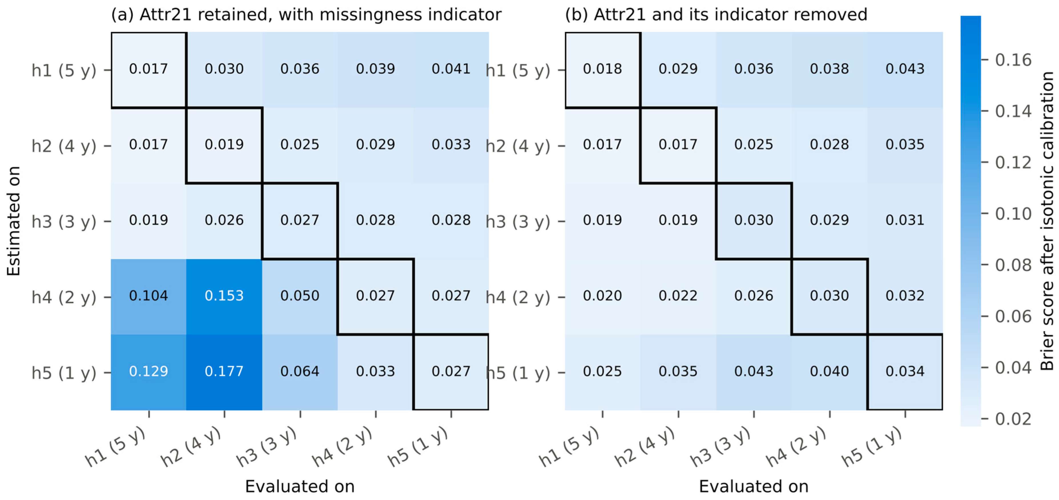
Figure 2.
Relative standard deviation of the CVaR estimate of the optimal allocation against the number of scenarios, over 40 independent samples per point (log–log). The dashed line marks the count adopted, m = 20,000.
Figure 2.
Relative standard deviation of the CVaR estimate of the optimal allocation against the number of scenarios, over 40 independent samples per point (log–log). The dashed line marks the count adopted, m = 20,000.
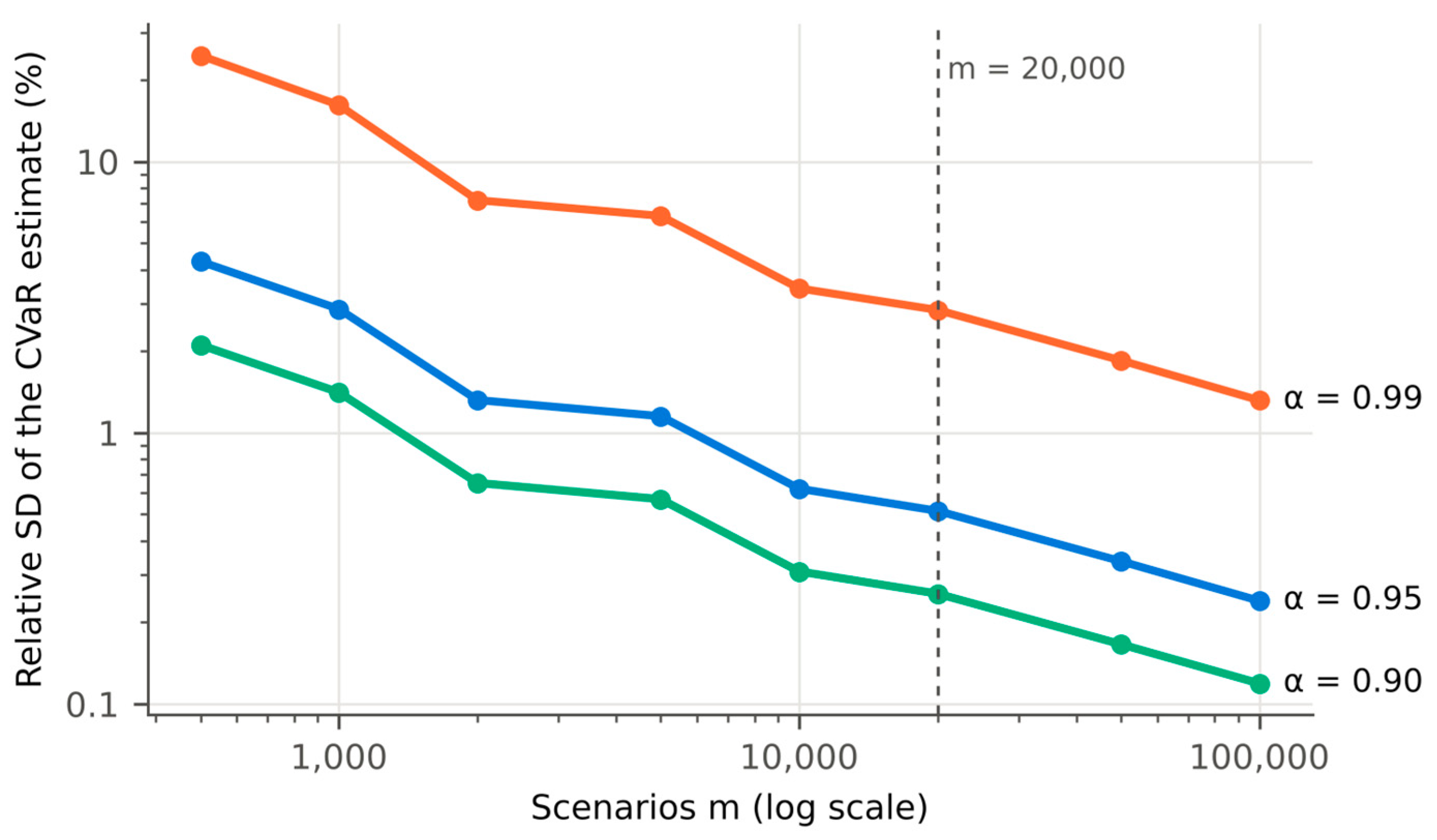
Figure 3.
Expected profit against tail profit (the negative of the CVaR of loss) out of sample, primary dataset, means over 30 samples with 95 per cent confidence intervals (smaller than the markers). Up and to the right is better on both axes.
Figure 3.
Expected profit against tail profit (the negative of the CVaR of loss) out of sample, primary dataset, means over 30 samples with 95 per cent confidence intervals (smaller than the markers). Up and to the right is better on both axes.
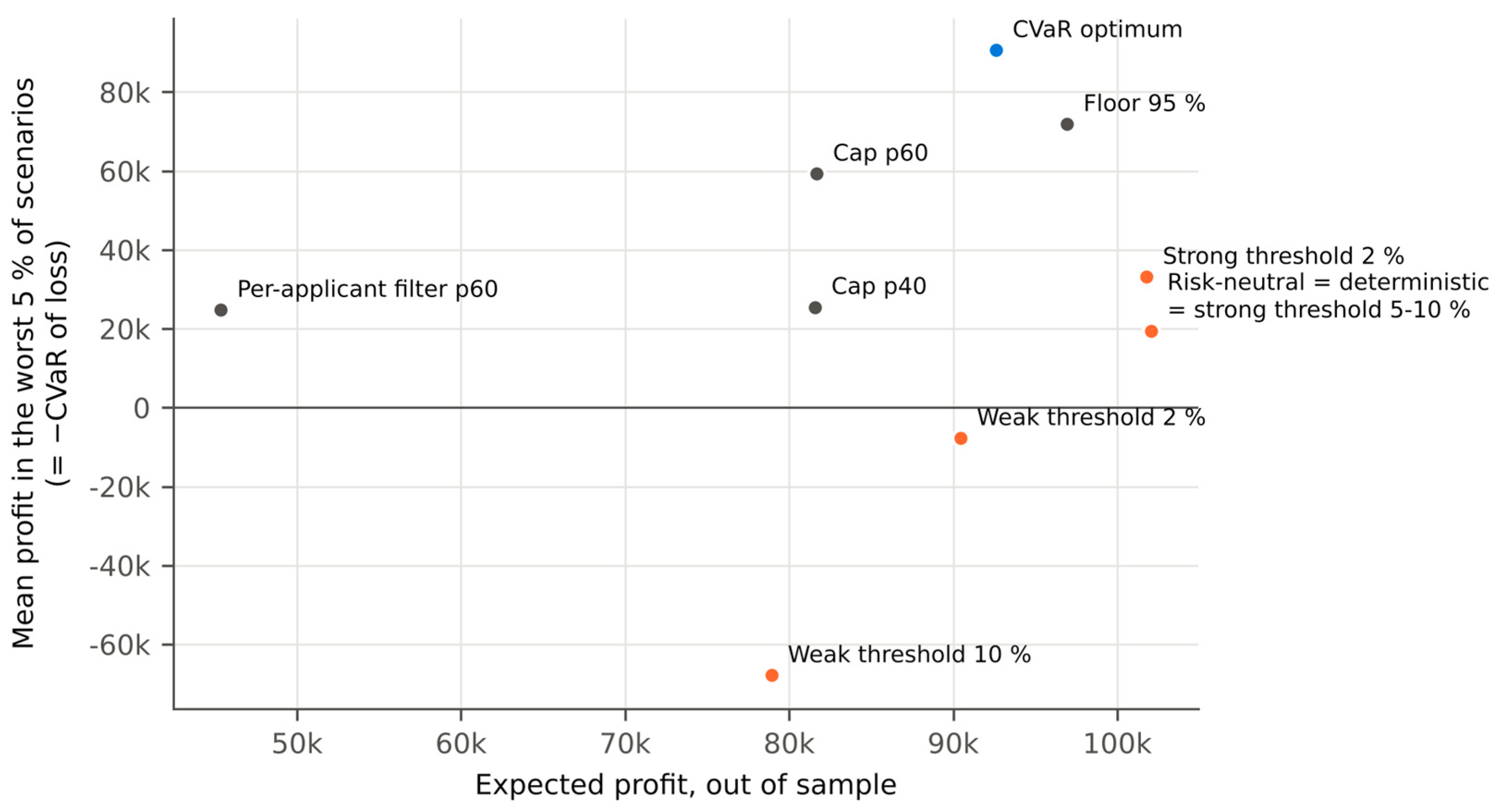
Figure 4.
Expected profit and tail profit under the stability cap and the per-applicant filter, primary dataset, out of sample.
Figure 4.
Expected profit and tail profit under the stability cap and the per-applicant filter, primary dataset, out of sample.
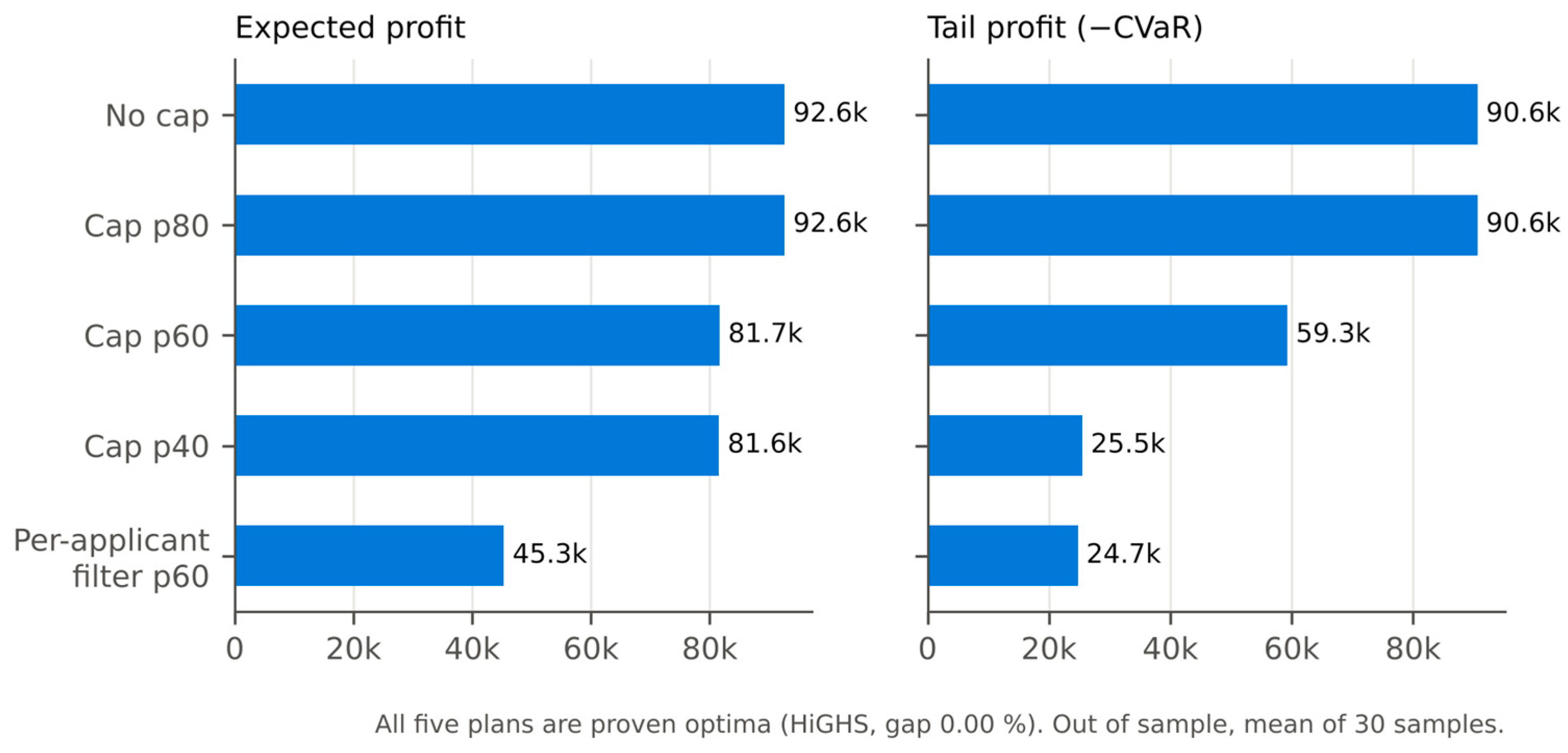
Table 3.
Risk model on the primary dataset, within horizon.
| Horizon | Base rate | AUC | Brier, raw | Brier, isotonic | Top decile, predicted | Top decile, observed |
| 1 | 0.038 | 0.945 | 0.0204 | 0.0177 | 0.161 | 0.198 |
| 2 | 0.039 | 0.944 | 0.0181 | 0.0179 | 0.284 | 0.265 |
| 3 (base case) | 0.047 | 0.922 | 0.0290 | 0.0270 | 0.357 | 0.318 |
| 4 | 0.053 | 0.916 | 0.0282 | 0.0264 | 0.302 | 0.277 |
| 5 | 0.069 | 0.953 | 0.0255 | 0.0259 | 0.518 | 0.562 |
Table 4.
The horizon ladder under three treatments of Attr21. Brier score after isotonic calibration; the off-horizon columns range over the twenty off-diagonal cells.
Table 4.
The horizon ladder under three treatments of Attr21. Brier score after isotonic calibration; the off-horizon columns range over the twenty off-diagonal cells.
| Ladder | AUC within horizon | Brier within horizon | Worst off-horizon Brier | Estimated at horizons 4–5, evaluated at 1–2 |
| Sentinel and indicator (version 1.1) | 0.916–0.953 | 0.018–0.027 | 0.178 | 0.112–0.178 |
| Single median rule and indicator (adopted) | 0.917–0.948 | 0.017–0.028 | 0.177 | 0.104–0.177 |
| Attr21 and indicator removed (robustness) | 0.904–0.947 | 0.018–0.034 | 0.043 | 0.020–0.035 |
Table 5.
Relative standard deviation (%) of the CVaR estimate of a fixed allocation over 40 independent samples.
Table 5.
Relative standard deviation (%) of the CVaR estimate of a fixed allocation over 40 independent samples.
| m | α = 0.90 | α = 0.95 | α = 0.99 |
| 1,000 | 1.41 | 2.86 | 16.15 |
| 5,000 | 0.57 | 1.15 | 6.31 |
| 20,000 | 0.26 | 0.52 | 2.84 |
| 100,000 | 0.12 | 0.24 | 1.32 |
Table 6.
Re-anchoring the scenario count. Relative standard deviation of the CVaR estimate at α = 0.95 over 40 independent samples per point, and the implied constant c = RSD × √m. The rule is anchored on the last three rows, m ≥ 20,000.
Table 6.
Re-anchoring the scenario count. Relative standard deviation of the CVaR estimate at α = 0.95 over 40 independent samples per point, and the implied constant c = RSD × √m. The rule is anchored on the last three rows, m ≥ 20,000.
| m | Relative standard deviation (%) | c |
| 500 | 4.281 | 95.7 |
| 1,000 | 2.859 | 90.4 |
| 2,000 | 1.320 | 59.0 |
| 5,000 | 1.151 | 81.4 |
| 10,000 | 0.622 | 62.2 |
| 20,000 | 0.515 | 72.8 |
| 50,000 | 0.336 | 75.1 |
| 100,000 | 0.240 | 75.9 |
Disclaimer/Publisher’s Note: The statements, opinions and data contained in all publications are solely those of the individual author(s) and contributor(s) and not of MDPI and/or the editor(s). MDPI and/or the editor(s) disclaim responsibility for any injury to people or property resulting from any ideas, methods, instructions or products referred to in the content. |
© 2026 by the authors. Licensee MDPI, Basel, Switzerland. This article is an open access article distributed under the terms and conditions of the Creative Commons Attribution (CC BY) license (http://creativecommons.org/licenses/by/4.0/).
Copyright: This open access article is published under a Creative Commons CC BY 4.0 license, which permit the free download, distribution, and reuse, provided that the author and preprint are cited in any reuse.