
Submitted:
23 October 2026
Posted:
26 October 2026
You are already at the latest version
Abstract
To address redundant motion caused when centrally scheduled multi-AGV systems continue executing stale commands during temporary communication interruptions, this paper proposes Continuity-Aware Multi-stage Preloading (CAMP). In the offline phase, SearchTeacher generates multi-stage supervision of relative vehicle priorities through look-ahead candidate evaluation, which is used to train a Context-Aware Gated Recurrent Unit (CA-GRU). When central communication is available, the frozen CA-GRU predicts stage-wise vehicle priorities and continuous task parameters; a constraint-aware decoder combines stage reachability, energy states, and role budgets to generate multi-stage task packets with explicit validity intervals and write them to local caches. During a communication interruption, vehicles execute the cached tasks locally stage by stage. System-level experiments with 30 independent random seeds and five interruption durations show no statistically significant difference between CAMP and SingleStep in longest continuous service, while total travel distance, relative energy consumption, and the mean number of moving AGVs are reduced by 69.5%, 71.1%, and 73.6%, respectively. The final frozen CA-GRU achieves 98.71% pairwise ranking accuracy on an independent test set, and CAMP achieves an approximately 31.8× speedup in task-packet generation relative to SearchTeacher. These results show that CAMP can maintain service continuity comparable to SingleStep while substantially reducing fleet motion and online computational cost under the tested communication-interruption conditions.
Keywords:
multi-AGV scheduling
; communication interruption
; multi-stage task preloading
; gated recurrent unit
; constraint-aware decoding
1. Introduction
Centralized multi-AGV systems are widely used in intelligent warehousing and flexible manufacturing because global state information can support coordinated task allocation and scheduling [1,2,3]. Such systems rely on central communication links for state reporting and command delivery, but these links may become temporarily unavailable in practice [4]. Unlike vehicle hardware failures, AGVs generally retain motion-control and local task-execution capabilities during a communication interruption, even though new central scheduling information is unavailable. If vehicles continue executing the last single-step commands received before disconnection, those commands become progressively stale as task locations and vehicle states evolve, potentially causing unnecessary travel and energy consumption.
Existing multi-AGV scheduling research mainly addresses task allocation, path coordination, and dynamic scheduling using mathematical optimization, heuristic, or metaheuristic methods [5,6,7,8,9]. Look-ahead scheduling further incorporates future tasks or state evolution to improve decisions in dynamic environments [10,11]. These approaches, however, generally depend on periodic state updates and command delivery. Related studies have examined task allocation under communication constraints or imperfect communication [12,13], cooperative control and data collection under intermittent connectivity [14,15], and rescheduling after sudden AGV failures [16]. Although these studies provide an important basis for multi-robot operation under abnormal communication conditions, few directly address how centrally generated scheduling information can continue to guide vehicle execution during temporary disconnection while limiting redundant motion caused by stale commands.
A direct strategy is to cache multiple future tasks while communication is available, thereby extending the time span over which scheduling information remains usable after disconnection. However, a longer cache does not necessarily imply better future tasks. As the prediction horizon increases, task location, vehicle state, reachability, and remaining energy may change; simply copying the current task or applying fixed stage transformations can therefore produce vehicle selections that are unsuitable for later predicted states. Multi-stage preloading must consequently provide both temporal coverage and stage-specific adaptation to predicted operating conditions.
Learning-based methods offer a way to reduce the online cost of such look-ahead decisions. Deep reinforcement learning has been applied to coordinated production-logistics scheduling, fleet management, energy-aware scheduling, and multi-AGV cooperative scheduling [17,18,19,20]. Multi-robot task-allocation studies have also used Monte Carlo tree search for online planning [21,22], distributed allocation under communication constraints [23], and swarm-intelligence or multi-objective optimization for complex assignment problems [24,25,26,27]. For the stage-wise role-allocation problem considered here, directly predicting discrete roles with a neural network would require the model to learn both relative vehicle value and deployment-constraint satisfaction. CAMP instead separates these functions by learning continuous relative priorities and enforcing reachability, energy, and role-budget constraints explicitly during decoding.
To address these issues, this paper proposes Continuity-Aware Multi-stage Preloading (CAMP), integrating look-ahead supervision, learned relative-priority prediction, and constraint-aware task generation. SearchTeacher evaluates a finite candidate set under predicted states and converts look-ahead vehicle-selection relationships into continuous relative-priority supervision. CA-GRU learns this mapping so that online candidate search can be replaced by lightweight inference, while a deterministic decoder enforces stage reachability, energy conditions, and role budgets. The resulting task packet contains stage-specific roles, spatial targets, and validity intervals and is cached locally whenever the corresponding central link is available. The study evaluates CAMP under fixed and randomized interruption timing and different preload depths, with emphasis on whether finite-horizon preloading can preserve service continuity while reducing redundant motion and online computation.
2. Materials and Methods
2.1. System Model and Problem Formulation
2.1.1. Centralized Multi-AGV System
Consider a dynamic task-service system consisting of one central scheduler and N AGVs. The AGV set is defined as
= {v1,v2,…,vN}
At time t, the observable state of AGV i is denoted by xi(t), which includes the vehicle position pi(t), remaining energy ei(t), current task role, and other local state information relevant to scheduling. The overall system observation is written as
The position of the dynamic service task is denoted by
pT(t) ∈ ℝ2
The dynamic task state evolves over time. Whenever the corresponding per-vehicle central command link is available, the central scheduler obtains the vehicle and task states, generates vehicle roles and spatial targets from the current trusted observations, and sends them to AGVs with available links.
At the scheduling layer, each AGV can take one of three task roles:
ri(t) ∈ = {Execute,Reserve,Standby}
Here, Execute denotes a vehicle currently providing the actual task service; Reserve denotes a vehicle retained to support future service or role switching; and Standby denotes a vehicle that currently has no current service or protection responsibility. Let the effective service range of AGV i be Ri; its distance to the dynamic task is
Only an AGV assigned the Execute role, located within the effective service range, and with remaining energy greater than 0 is counted as an actual service vehicle. The corresponding single-vehicle service indicator is defined as
where 𝕀[⋅] is the indicator function. The system-level effective service state is
si(t) = 𝕀[ri(t) = Execute ∧ di(t) ≤ Ri ∧ ei(t) > 0]
The system architecture is shown in Figure 1; central communication availability and the unified forced-blackout mechanism are described in Section 2.1.2.
2.1.2. Central Communication Blackout Model
Define the unified forced-blackout state variable
A single continuous communication blackout is represented by the time interval
where tb and te denote the blackout start and end times, respectively, and the blackout duration is
= {t∣tb ≤ t < te}
Tb = te − tb
In addition to the unified forced blackout, each AGV has an independent deterministic central communication window. At simulation initialization, this window is constructed from the baseline service windows: the start of each service interval is extended 30 s earlier and the end is extended 15 s later; the resulting intervals are clipped to [0,T], overlapping or adjacent intervals are merged, and the unified forced-blackout interval is removed. Subsequent online adjustments to the service windows do not alter the central communication windows already generated.
Therefore, when t∈, no AGV can communicate with the central scheduler. Outside , each AGV uploads states and receives tasks only within its own central communication windows. When a link is unavailable, the central side extrapolates from the vehicle’s most recently reported state, while the vehicle continues executing locally stored tasks. Because the per-vehicle communication windows differ, the most recent successful task-reception time may also differ across vehicles.
This paper studies the unified forced blackout superimposed on the deterministic per-vehicle communication windows described above; related communication-cooperation mechanisms can be found in [28].
2.1.3. Multi-Stage Local Task Representation
At decision time tk, CAMP generates a task packet containing H stages,
where H is the number of preloaded stages. Let the duration of each stage be ΔTp; the nominal preload horizon of a task packet is therefore
(tk) = {π(1),π(2),…,π(H)}
Tp = HΔTp
The validity interval corresponding to stage h is
(h) = [tk + (h − 1)ΔTp, tk + hΔTp) h = 1,…,H.
A stage task contains the role, spatial target, local action, and stage validity interval for each AGV. Specifically, the task-parameter vector of AGV i at stage h is
where is the role, is the trajectory look-ahead parameter, is the angular offset, and is the service-distance ratio. Given a predicted trajectory of the dynamic task, these continuous parameters are further decoded into the vehicle spatial target position .
The task at stage h can be written as
For each stage, the numbers of Execute and Reserve vehicles are constrained by deployment budgets:
where and are the maximum deployment counts for the Execute and Reserve roles, respectively.
Task assignment must also satisfy stage reachability and energy-authorization conditions. Let denote the reachability margin of AGV i relative to the target position at stage h; then
The feasibility condition is
where Δc is the coverage safety margin, vmax is the maximum AGV speed, and and are the vehicle position and predicted task position at stage h, respectively. Satisfying this condition means that the vehicle can reach the admissible region under the motion constraints of the corresponding stage. Let the predicted energy state at the stage be and the minimum authorized energy be emin; then any vehicle assigned an Execute or Reserve task must satisfy
2.1.4. Performance Metrics and Problem Formulation
Let the system operating horizon be T. Based on the service state in Equation (7), the cumulative effective service time is defined as
The longest continuous service time is defined as the longest continuous interval during which the system maintains S(t) = 1:
The total vehicle travel distance is defined as
Relative energy consumption is represented by the cumulative decrease in the normalized AGV energy states:
To remain consistent with the simulation implementation, vehicle mobility is measured from position changes between adjacent decision instants. Let the decision instants be t_k=kΔt (k=0,…,K−1), and let ε_p be the displacement threshold used to exclude numerical rounding errors. The number of moving AGVs during decision interval k is
The mean number of moving AGVs is defined as a duration-weighted average over decision intervals:
To characterize the temporal validity of scheduling information, define the expired-command indicator I_exp,i(t_k) for AGV i at decision instant t_k. For SingleStep, I_exp,i(t_k)=1 when the vehicle has no valid central command or the age of the most recent successfully delivered command exceeds 50 s. For multi-stage preloading methods, I_exp,i(t_k)=1 when the local task packet is invalid or the current time has exceeded the enabled preload horizon. The expired-command rate is computed over discrete samples of all AGVs and all decision instants as
Command expiration only indicates that the scheduling information has lost its temporal validity; the vehicle still holds the last locally valid action. For multi-stage preloading methods, when the local task packet is invalid or the stage index exceeds the number of enabled stages, I_uncov,i(t_k)=1. The corresponding task-packet uncovered rate is
where K is the number of decision intervals in the simulation.
Under the above metrics and constraints, this work focuses on maintaining service continuity during temporary central communication blackouts while reducing vehicle motion, energy consumption, and scheduling-information invalidation. The multi-objective formulation is
subject to
where Ωreach, Ωenergy, and Ωrole denote the feasible sets defined by stage reachability, energy authorization, and role budgets, respectively.
(tk) ∈ Ωreach ∩ Ωenergy ∩ Ωrole,
CAMP approximately solves the above problem through offline look-ahead supervision, online priority prediction, and constraint-aware decoding; the detailed method is given in Section 2.2.
2.2. CAMP Method
2.2.1. Overall Framework
CAMP consists of three parts: offline supervision generation, online multi-stage task generation, and local execution during communication blackouts. As shown in Figure 2, in the offline phase SearchTeacher generates multi-stage relative-priority supervision for vehicles through finite-candidate look-ahead search and uses it to train CA-GRU; in the online phase, the frozen CA-GRU predicts vehicle priorities and continuous task parameters for each stage, after which constraint-aware decoding generates the multi-stage task packet.
The task packet is written only to the local caches of vehicles whose central command links are currently available. After a communication blackout, each vehicle executes the cached tasks stage by stage according to the time at which it most recently received a task packet successfully, thereby maintaining local task updates within the finite preload horizon.
2.2.2. SearchTeacher Relative-Priority Supervision Generation
SearchTeacher is used to generate offline supervision for CA-GRU. Rather than directly providing Execute, Reserve, and Standby classification labels, it forms continuous relative priorities for vehicles through look-ahead evaluation of candidate configurations.
For stage h, let the finite candidate set constructed from the current predicted system state be
where M is the number of candidates. The candidate set is constructed by combining a deterministic baseline strategy, provisional perturbations to the Execute count, and different look-ahead modes. The provisional Execute count is used only for teacher search and does not change the role budget in online decoding. The specific candidate configurations are given in Section 3.
Starting from the current stage, SearchTeacher evaluates candidates in a rolling manner. At each stage it selects the candidate action with the highest discounted cumulative score and then advances the internal predicted state to the next stage.
The single-stage score can be expressed as
Jl = wsSl + wcCl + wrRl − weEl − wswNsw,l − wuUl
The six evaluation terms represent, in order, the service state, continuous-service indicator, redundancy-protection indicator, energy cost, number of role switches, and service-uncovered indicator; the corresponding weights are given by the parameters in the equation. The rolling total score is
where γ is the discount factor; the specific score weights and discount setting are given in Section 3.
SearchTeacher thereby performs look-ahead evaluation that balances service continuity, redundant protection, and resource cost.
The candidate with the highest score is denoted by
where the score represents the discounted cumulative value of the candidate from stage h onward.
SearchTeacher further forms the vehicle-priority vector from the candidate-search results,
where the priority represents only the relative scheduling order among vehicles and does not directly correspond to role classes.
A training sample consists of the current decision-context vector and the multi-stage continuous supervision produced by SearchTeacher:
Thus, each training sample contains the current decision context and its corresponding multi-stage continuous supervision.
2.2.3. CA-GRU Relative-Priority Learning
CA-GRU learns the mapping from the current decision context to multi-stage continuous outputs. The model does not explicitly stack historical observations across decision instants; instead, based on the same current context, information is recursively passed between preload stages through the GRU hidden state.
The model consists of a per-feature attention module and a single-layer GRU. The current context is first processed by per-feature attention gating to obtain a weighted representation, which is then fed to the GRU together with stage encoding; the hidden state is recursively propagated between adjacent preload stages. At each stage, the model outputs a relative priority and continuous task parameters for every AGV for subsequent constraint-aware decoding.
Let the scheduling context available at decision instant t_k be denoted by O(t_k). The input features comprise system-level task and communication states together with per-vehicle motion, information age, coverage margin, and recent-task information. A fixed mapping gives
where φ(·) denotes feature concatenation, scale normalization, and standardization. The standardization parameters are estimated only from the training set and remain fixed for validation, testing, and online inference. The input uses only information available at the current decision instant and contains neither the true future trajectory nor the actual blackout duration. From the current task state and motion model, the scheduler separately constructs future stage-wise task-position predictions,
Equation (38) is obtained by rolling the current state forward and does not access the true future trajectory in the simulation environment. It is used mainly for SearchTeacher’s rolling evaluation and for reachability and spatial-target decoding in Section 2.2.4; CA-GRU itself uses only the current context and stage encoding.
Denote the frozen CA-GRU by f_θ, where θ represents the model parameters. For AGV i and stage h, its predicted relative priority is
This yields the stage-wise priority vector
CA-GRU outputs continuous relative priorities and task parameters, while the final roles are determined by the feasibility screening and constraint-aware decoding in Section 2.2.4.
Training uses the continuous priorities from SearchTeacher as supervision and imposes a margin-based pairwise ranking constraint on ordered AGV pairs whose teacher-priority difference exceeds a threshold. The set of valid vehicle pairs is defined as
where the threshold is used to retain vehicle pairs with clear ranking relationships. The pairwise ranking loss is
Equation (42) uses a squared hinge form and computes a squared penalty for ranking-margin violations only on ordered vehicle pairs with unambiguous teacher rankings.
The total loss consists of a weighted regression loss, a pairwise ranking loss, and a stage-change consistency loss. The weighted regression loss averages across stages, vehicles, and continuous output channels with configurable weights:
where C is the number of continuous output channels and each channel uses an adjustable weight. The stage-change consistency loss matches priority increments between adjacent stages and is defined as
The total training loss is defined as
= reg + λrankrank + λtranstrans
Model training uses an independent validation set to select the frozen checkpoint and jointly considers regression error, pairwise ranking accuracy, and Top-K set recovery capability; the specific training configuration is given in Section 3.
2.2.4. Constraint-Aware Multi-Stage Decoding
The continuous priorities and task parameters output by CA-GRU must be further converted into deployable tasks. At every predicted stage, CAMP rechecks vehicle feasibility and assigns the Execute, Reserve, and Standby roles according to priority.
According to Equations (18)–(20), the reachability margin and predicted energy of each AGV are calculated from the current internal predicted state and the stage task position, and the stage-feasibility indicator is defined as
The corresponding feasible AGV set is
Within the feasible set, vehicles are sorted in descending order of predicted priority, and the Execute set is constructed sequentially under the role-budget constraint,
The Reserve set is then constructed from the remaining feasible vehicles,
All remaining vehicles enter the Standby set,
h = {vi ∈ ∣vi ∉ h, vi ∉ h}
After the roles are determined, the decoder combines the predicted stage task position and continuous task parameters to generate spatial targets. If no vehicle simultaneously satisfies the reachability and energy conditions at the current stage, a deterministic fallback score composed of reachability margin and remaining energy is used to select a candidate; the specific score weights are given in Section 3.
After stage h is completed, the internal predicted state is rolled forward to the next stage and the task position, vehicle states, and deployment feasibility are recomputed. Thus, multi-stage tasks are generated stage by stage from predicted states rather than by simply copying the current roles.
The online constraint-aware multi-stage decoding procedure is given in Algorithm 1.
| Algorithm 1. CAMP constraint-aware multi-stage task generation |
|
Input: current system state X(tk); frozen CA-GRU fθ; number of preload stages H; stage duration ΔTp; Execute budget ; Reserve budget ; minimum energy threshold emin Output: multi-stage task packet (tk)1. Initialize the internal predicted state , (tk) ← ⌀. 2. Construct the CA-GRU context input Z_k from the current observation. 3. for h = 1,…,H do4. Update the predicted task position for stage h.5. Use fθ to compute .6. Compute and for each AGV. 7. Obtain the feasible set according to Equations (46)–(47).8. Sort feasible AGVs in descending order of .9. Determine h under the constraint.10. Determine h from the remaining feasible vehicles according to . 11. Assign all remaining vehicles to h.12. Generate from the stage task position and continuous task parameters. 13. If no feasible vehicle exists, select a candidate using the deterministic fallback score. 14. Form the stage task π(h) and add it to (tk). 15. Roll the internal predicted state forward to the next stage. 16. end for 17. return (tk) |
2.2.5. Local Stage-Wise Execution During Communication Blackouts
A multi-stage task packet is generated at a decision instant when at least one central command link is available, but only the task component corresponding to vehicles whose links are available at that instant is written to their local caches; vehicles with unavailable links retain their previous caches. Consequently, the most recent successful task-packet reception time may differ among AGVs. During communication-limited operation, each vehicle selects its current stage according to the age of its local task packet; when communication is restored, newly received tasks overwrite the old cache.
For
the current stage index is
tk ≤ t < tk + HΔTp
AGV i reads the role and spatial target corresponding to the current stage from its local cache and continues execution using its local motion controller.
As shown in Figure 3, the stages of a task packet correspond to consecutive validity intervals, allowing a vehicle to switch its local role and spatial target stage by stage after communication becomes unavailable.
When a communication blackout exceeds the nominal preload horizon, the local cache no longer contains new stage tasks and the vehicle holds the last valid action. Its execution logic after disconnection is
where the former denotes the local execution action corresponding to stage h, and the latter denotes the last valid action before the end of the preload horizon.
Therefore, CAMP executes stage-wise tasks within the preload horizon and transitions to a last-action-hold state beyond that horizon.
3. Results
This section evaluates CAMP in terms of experimental setup, priority learning and multi-stage task preloading, system performance under communication blackouts, and online computational efficiency. The formal system-level experiments use 30 independent random seeds, and different methods are compared in pairs under the same random seed.
3.1. Experimental Setup
We construct a centralized two-dimensional dynamic logistics service scenario in which the continuously moving task point pT(t) represents the dynamic service demand. The system contains eight AGVs and four access points (APs); the spatial configuration and baseline task trajectory are shown in Figure 4. In the formal experiments, random perturbations are applied to the initial AGV positions and the initial task-point state. Under the same random seed and communication-blackout configuration, all four methods share identical vehicle initial states, task trajectories, and communication conditions to ensure paired comparison. AP-network availability windows are used only to evaluate service-chain value; the central command link does not model propagation fading based on AGV–AP geometric distance, and the per-vehicle central communication windows are generated as defined in Section 2.1.2.
Random initial-state perturbations are added to the baseline motion model of the dynamic task trajectory, and at t=330 s the velocity direction is rotated by 60° to create a service trajectory with a state change. Online trajectory prediction uses a weighted fusion of constant-velocity, coordinated-turn, and weak-acceleration models, rolled forward from the current observable state over a 180 s prediction horizon without accessing the true future trajectory. Prediction uncertainty consists of a time-growth term and inter-model dispersion. The detailed trajectory, perturbation, and prediction parameters are listed in Table 1.
The total simulation duration is 600 s with a 30 s decision interval. The fixed unified forced blackout is centered at approximately 330 s, with durations of 60, 120, 180, 240, and 300 s. CAMP uses three preload stages of 60 s each, yielding a nominal preload horizon of 180 s; the 240 s and 300 s cases are used to examine performance when the blackout exceeds the preload horizon. Each configuration uses 30 independent random seeds. In the randomized-blackout robustness experiment, only the start time of the unified forced blackout is randomized; for a given random seed and blackout duration, all methods use the same blackout interval.
The system-level comparison includes Autonomous, SingleStep, RulePreload, and CAMP. Autonomous regenerates the action from the current true scene at every decision instant and ignores the central communication windows, serving as a full-information reference. SingleStep refreshes the single-step action only when the corresponding vehicle’s central link is available and otherwise holds the most recently received action. RulePreload and CAMP use the same 3×60 s local-cache framework, but RulePreload applies fixed stage-wise role transitions based on the UtilityGreedyThreeRole baseline action; CAMP uses CA-GRU to predict relative priorities and continuous task parameters and generates multi-stage tasks subject to stage reachability, energy, and role budgets. When at least five vehicles are available, the three RulePreload stages use 3 Execute + 2 Reserve, 0 Execute + 5 Reserve, and 5 Execute + 0 Reserve vehicles, respectively. RulePreload therefore serves as a rule-based multi-stage preloading reference rather than a strict ablation of an internal CAMP component.
The CA-GRU training data are generated from 120 independent scenarios, yielding 2040 samples, and are divided by scenario into training, validation, and test sets with no scenario overlap. The training data and formal system-level evaluation use mutually independent random seeds, and the final frozen model is selected using the validation composite metric S_val. The main experimental and implementation parameters are summarized in Table 1, and method comparisons use paired samples under identical random seeds. Because the paired differences in some configurations do not satisfy the normality assumption, two-sided Wilcoxon signed-rank tests are used throughout at a significance level of α=0.05, and 95% confidence intervals for paired differences are reported.
3.2. Effectiveness of Learning and Multi-Stage Task Preloading
CA-GRU learns the relative vehicle priorities generated by SearchTeacher rather than directly predicting discrete roles. Figure 5 shows the training and validation convergence of the model. The system-level experiments use the frozen model that achieves the best validation composite metric Sval. On the independent test set, this model achieves a pairwise ranking accuracy of 98.71%, Execute Top-K and Protect Top-K recall rates of 96.16% and 98.27%, respectively, and a Spearman rank correlation coefficient of 0.629. The high pairwise ranking accuracy and Top-K recall indicate that the model can effectively recover the high-priority vehicle sets needed for subsequent role-budget decoding.
For Top-K, K is determined dynamically according to the number of teacher-assigned roles in each sample and stage: Execute Top-K uses the number of teacher Execute vehicles, whereas Protect Top-K uses the total number of teacher Execute and Reserve vehicles.
The ablation results for the number of preload stages are shown in Figure 6 and Table 2. As preload depth increases, the task-packet uncovered rate decreases markedly, whereas relative energy consumption does not increase monotonically. Under a 180 s communication blackout, the uncovered rate decreases from 39.38% with one stage to 23.12% with two stages and 11.25% with three stages; under a 300 s blackout, it decreases from 56.88% to 43.12% and 33.12%, respectively. Therefore, the subsequent system-level experiments use the three-stage configuration.
3.3. System Performance Under Communication Blackouts
3.3.1. Service Continuity
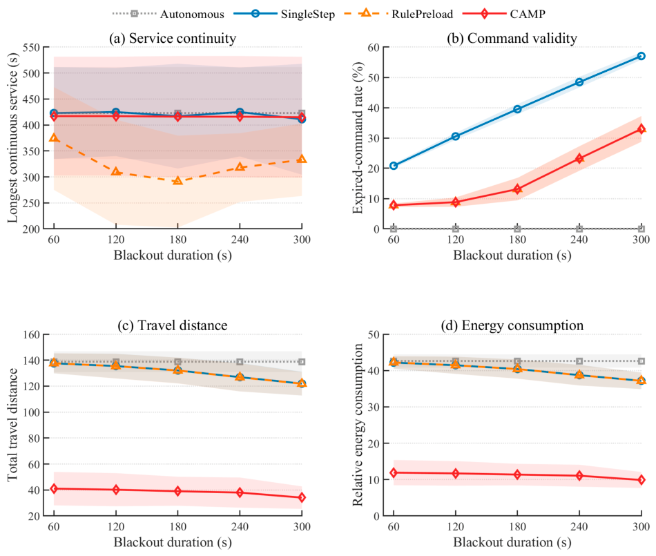
Figure 7 shows the service continuity of the four methods under different communication-blackout durations. Autonomous remains essentially stable; SingleStep and CAMP maintain high service continuity under all five blackout durations, whereas the longest continuous service of RulePreload decreases markedly as the blackout duration increases.
Across the 30 paired samples for each blackout duration, no statistically significant difference in longest continuous service is detected between CAMP and SingleStep. The two-sided Wilcoxon signed-rank test yields p-values of 0.383–1.000, and all 95% confidence intervals for paired differences include 0.
3.3.2. Command Timeliness and Resource Efficiency
Figure 8 and Table 3 further compare command timeliness and resource consumption. Aggregated over the five blackout durations, the mean longest continuous service is 419.8 s for SingleStep and 414.8 s for CAMP. Meanwhile, CAMP reduces the mean number of moving AGVs from 4.81 to 1.27, the total travel distance from 129.30 to 39.43, and relative energy consumption from 39.60 to 11.44, corresponding to reductions of 73.6%, 69.5%, and 71.1%, respectively. Thus, the main advantage of CAMP is reduced vehicle motion and resource consumption rather than a further increase in continuous service time.
The mean expired-command rate is 16.63% for both CAMP and RulePreload, lower than the 39.38% of SingleStep. The expired-command rate reflects only the temporal validity of scheduling information; after a command is marked as expired, the vehicle still holds the last locally available action.
In the paired comparison for each of the five blackout durations, relative to SingleStep, CAMP reduces the expired-command rate by 41.76%–73.47%, total travel distance by 66.29%–71.60%, and relative energy consumption by 67.91%–73.12%. Two-sided Wilcoxon tests for all of these resource and information-timeliness metrics reach statistical significance, and the corresponding 95% confidence intervals for paired differences do not include 0. In contrast, although RulePreload reduces the expired-command rate, its mean number of moving AGVs and relative energy consumption remain close to those of SingleStep while its continuous service decreases substantially.
Detailed results for each fixed blackout duration are provided in Table A1 in Appendix A.
3.3.3. Robustness to Randomized Unified Forced-Blackout Timing
To test whether the results depend on fixing the center of the unified forced blackout at approximately 330 s, the blackout start time is further randomized while all other experimental conditions remain unchanged. Under the same random seed and blackout duration, the four methods use the same blackout interval.
After randomizing the blackout timing, no statistically significant difference in longest continuous service is detected between CAMP and SingleStep. Meanwhile, CAMP reduces the expired-command rate by 42.18%–71.13%, total travel distance by 70.06%–72.02%, relative energy consumption by 71.42%–73.40%, and the mean number of moving AGVs by 73.37%–74.92%; the corresponding paired tests are all statistically significant. These results are consistent with the overall trend of the fixed-blackout experiments, indicating that the main conclusions do not depend on fixing the unified forced-blackout center at 330 s.
Figure 9.
Robustness comparison of the four methods under randomized unified forced-blackout timing.
Figure 9.
Robustness comparison of the four methods under randomized unified forced-blackout timing.
3.4. Online Computational Efficiency
Figure 10 compares the end-to-end task-packet generation times of SearchTeacher and CAMP. The timing test was implemented in MATLAB and repeated 20 times after warm-up on a workstation equipped with an Intel Xeon E5-2680 v4 CPU and 64 GB RAM. The mean task-packet generation time is 0.5296±0.0170 s for SearchTeacher and 0.01666±0.00354 s for CAMP, so CAMP requires approximately 1/31.79 of the SearchTeacher time, corresponding to a speedup of about 31.8×. Their maximum generation times are 0.5654 s and 0.02534 s, respectively, both below the 30 s system decision period.
The computational difference mainly arises because SearchTeacher performs multi-stage rolling evaluation over candidate configurations, whereas online CAMP requires only forward inference with the frozen CA-GRU and deterministic constraint-aware decoding. These timing results apply to the present eight-AGV, three-stage configuration; larger fleets and deeper preload horizons require separate evaluation.
4. Discussion
The results indicate that CAMP’s main benefit lies in resource efficiency rather than extending service duration. Under both fixed and randomized unified forced blackouts, no statistically significant difference in longest continuous service was detected between CAMP and SingleStep, whereas CAMP substantially reduced travel distance, relative energy consumption, and fleet mobility. This behavior is consistent with the design of CAMP: instead of holding a single pre-disconnection action, the method uses stage-wise relative priorities together with explicit feasibility and role constraints to limit unnecessary vehicle activity as predicted task conditions evolve. The expired-command rate should therefore be interpreted as an information-timeliness metric rather than a direct measure of service continuity.
The preload-depth study further shows that additional stages primarily extend the temporal coverage of scheduling information. RulePreload provides a useful reference because it uses the same nominal cache horizon without learned priority prediction, yet it does not reproduce CAMP’s service-resource performance. However, RulePreload and CAMP differ simultaneously in vehicle selection, stage-wise role evolution, and decoding, so this comparison is not a strict component-wise ablation. Likewise, the observed 31.8× task-packet generation speedup applies to the current eight-AGV, three-stage configuration and should not be extrapolated quantitatively to larger fleets without further testing.
This study is a simulation-based system-level validation rather than a high-fidelity digital twin of a specific warehouse. Dynamic logistics demand is abstracted as a two-dimensional moving service point, and the communication model uses deterministic per-vehicle central communication windows with a superimposed unified forced blackout. Random packet loss, communication delay, independent vehicle disconnections, asynchronous reconnection, task-motion-model mismatch, road-network congestion, and heterogeneous fleets are not modeled explicitly. These factors define the main scope of future validation.
5. Conclusions
This paper proposed CAMP for multi-stage task preloading during temporary central communication interruptions. In system-level experiments with 30 independent random seeds, CAMP showed no statistically significant difference from SingleStep in longest continuous service, while reducing total travel distance, relative energy consumption, and the mean number of moving AGVs by 69.5%, 71.1%, and 73.6%, respectively, across the five fixed blackout durations. The final frozen CA-GRU achieved 98.71% pairwise ranking accuracy on the independent test set, and online task-packet generation achieved an approximately 31.8× speedup relative to SearchTeacher.
These results support finite-horizon multi-stage preloading as a practical way to reduce dependence on continuous central updates when vehicles retain local execution capability. Future work will examine stochastic communication impairments, task-motion-model mismatch, larger and heterogeneous fleets, and validation in high-fidelity digital twins and physical warehouse platforms.
Author Contributions
Conceptualization, Y.L. and J.Y.; methodology, Y.L.; software, Y.L.; validation, Y.L., C.X. and J.Z.; formal analysis, Y.L. and Z.J.; data curation, Y.L.; writing—original draft preparation, Y.L.; writing—review and editing, Y.L., C.X., J.Z., Z.J. and J.Y.; visualization, Y.L.; supervision, J.Y.; project administration, J.Y. All authors have read and agreed to the published version of the manuscript.
Funding
This research received no external funding.
Institutional Review Board Statement
Not applicable.
Informed Consent Statement
Not applicable.
Data Availability Statement
The data supporting the findings of this study are available from the corresponding author upon reasonable request.
Conflicts of Interest
The authors declare no conflicts of interest.
Appendix A

Table A1.
Detailed system performance of the four methods under the five fixed forced-blackout durations.
Table A1.
Detailed system performance of the four methods under the five fixed forced-blackout durations.
| Method | Blackout duration (s) | Cumulative effective service (s) | Longest continuous service (s) | Expired-command rate (%) | Total travel distance (model units) | Relative energy consumption | Mean number of moving AGVs |
| Autonomous | 60 | 423 | 423 | 0.00 | 138.81 | 42.63 | 5.13 |
| SingleStep | 60 | 422 | 422 | 21.25 | 137.13 | 42.09 | 5.07 |
| RulePreload | 60 | 408 | 374 | 7.50 | 137.25 | 42.15 | 5.07 |
| CAMP | 60 | 422 | 417 | 7.50 | 41.11 | 11.93 | 1.32 |
| Autonomous | 120 | 423 | 423 | 0.00 | 138.81 | 42.63 | 5.13 |
| SingleStep | 120 | 422 | 422 | 30.63 | 130.55 | 40.01 | 4.82 |
| RulePreload | 120 | 392 | 344 | 8.12 | 130.29 | 39.98 | 4.81 |
| CAMP | 120 | 421 | 416 | 8.12 | 40.88 | 11.90 | 1.32 |
| Autonomous | 180 | 423 | 423 | 0.00 | 138.81 | 42.63 | 5.13 |
| SingleStep | 180 | 417 | 417 | 39.38 | 125.19 | 38.38 | 4.64 |
| RulePreload | 180 | 381 | 335 | 11.25 | 125.10 | 38.38 | 4.63 |
| CAMP | 180 | 420 | 415 | 11.25 | 42.20 | 12.32 | 1.37 |
| Autonomous | 240 | 423 | 423 | 0.00 | 138.81 | 42.63 | 5.13 |
| SingleStep | 240 | 423 | 419 | 48.75 | 134.57 | 41.15 | 5.05 |
| RulePreload | 240 | 386 | 291 | 23.12 | 134.45 | 41.14 | 5.04 |
| CAMP | 240 | 420 | 415 | 23.12 | 38.22 | 11.06 | 1.23 |
| Autonomous | 300 | 423 | 423 | 0.00 | 138.81 | 42.63 | 5.13 |
| SingleStep | 300 | 423 | 419 | 56.88 | 119.05 | 36.36 | 4.49 |
| RulePreload | 300 | 375 | 292 | 33.12 | 119.05 | 36.38 | 4.48 |
| CAMP | 300 | 418 | 411 | 33.12 | 34.75 | 10.00 | 1.12 |
Note: Each row reports the mean over 30 independent random seeds for the corresponding method and forced-blackout duration. Energy consumption is reported on the relative model scale.
References
- Park, J.-S.; Kim, J.-W. Multi-AGV Scheduling under Limited Buffer Capacity and Battery Charging Using Simulation Techniques. Appl. Sci. 2024, 14, 1197. [CrossRef]
- Li, J.; Chen, Y.; Zhou, L.; Dong, R.; Yin, W.; Huang, W.; Zhang, F. Multi-AGV-Driven Pallet-Picking Scheduling Optimization (MADPSO): A Method for Flexible Multi-Level Picking Systems. Appl. Sci. 2024, 14, 1618. [CrossRef]
- Zhang, Z.; Chen, J.; Guo, Q. Application of Automated Guided Vehicles in Smart Automated Warehouse Systems: A Survey. Comput. Model. Eng. Sci. 2023, 134, 1529–1563. [CrossRef]
- Matos, D.; Costa, P.; Lima, J.; Costa, P. Multi AGV Coordination Tolerant to Communication Failures. Robotics 2021, 10, 55. [CrossRef]
- Ge, S.; Zhang, H.; Xu, Z.; Yang, Z. A Multi-Objective Artificial Bee Colony Algorithm Incorporating Q-Learning Search for the Flexible Job Shop Scheduling Problems with Multi-Type Automated Guided Vehicles. Appl. Sci. 2025, 15, 10948. [CrossRef]
- Xin, J.; Yuan, Q.; D’Ariano, A.; Guo, G.; Liu, Y.; Zhou, Y. Dynamic unbalanced task allocation of warehouse AGVs using integrated adaptive large neighborhood search and Kuhn–Munkres algorithm. Comput. Ind. Eng. 2024, 195, 110410. [CrossRef]
- Wu, S.; Xiang, W.; Li, W.; Chen, L.; Wu, C. Dynamic Scheduling and Optimization of AGV in Factory Logistics Systems Based on Digital Twin. Appl. Sci. 2023, 13, 1762. [CrossRef]
- Yu, C.; Liao, W.; Zu, L. Dynamic Scheduling Optimization Method for Multi-AGV-Based Intelligent Warehouse Considering Bidirectional Channel. Systems 2024, 12, 9. [CrossRef]
- Song, H.; Yang, S.; Yin, S.; Wang, J.; Xu, Z. Intelligent Scheduling of a Pulsating Assembly Flow Shop Considering a Multifunctional Automated Guided Vehicle. Appl. Sci. 2025, 15, 2593. [CrossRef]
- Kim, K.H.; Bae, J.W. A Look-Ahead Dispatching Method for Automated Guided Vehicles in Automated Port Container Terminals. Transp. Sci. 2004, 38, 224–234. [CrossRef]
- Wang, X.; Wu, W.; Xing, Z.; Zhang, T.; Niu, H. A look-ahead AGV scheduling algorithm with processing sequence conflict-free for a no-buffer assembly line. J. Adv. Mech. Des. Syst. Manuf. 2023, 17, JAMDSM0063. [CrossRef]
- Chen, Z.; Li, L.; Kan, Z. Distributed Task Allocation and Planning Under Temporal Logic and Communication Constraints. IEEE Robot. Autom. Lett. 2024, 9, 6536–6543. [CrossRef]
- Nayak, S.; Yeotikar, S.; Carrillo, E.; Rudnick-Cohen, E.; Jaffar, M.K.M.; Patel, R.; Azarm, S.; Herrmann, J.W.; Xu, H.; Otte, M.W. Experimental Comparison of Decentralized Task Allocation Algorithms Under Imperfect Communication. IEEE Robot. Autom. Lett. 2020, 5, 572–579. [CrossRef]
- Kantaros, Y.; Guo, M.; Zavlanos, M.M. Temporal Logic Task Planning and Intermittent Connectivity Control of Mobile Robot Networks. IEEE Trans. Autom. Control 2019, 64, 4105–4120. [CrossRef]
- Guo, M.; Zavlanos, M.M. Multirobot Data Gathering under Buffer Constraints and Intermittent Communication. IEEE Trans. Robot. 2018, 34, 1082–1097. [CrossRef]
- Wang, X.; Zou, W.; Meng, L.; Zhang, B.; Li, J.; Sang, H. Effective metaheuristic and rescheduling strategies for the multi-AGV scheduling problem with sudden failure. Expert Syst. Appl. 2024, 250, 123473. [CrossRef]
- Huang, X.; Chen, Y.; Yi, W.; Pei, Z.; Cheng, Z. Solving Collaborative Scheduling of Production and Logistics via Deep Reinforcement Learning: Considering Limited Transportation Resources and Charging Constraints. Appl. Sci. 2025, 15, 6995. [CrossRef]
- Dai, Y.; Kim, D.; Lee, K. Development of a Fleet Management System for Multiple Robots’ Task Allocation Using Deep Reinforcement Learning. Processes 2024, 12, 2921. [CrossRef]
- Zhang, F.; Li, R.; Gong, W. Deep reinforcement learning-based memetic algorithm for energy-aware flexible job shop scheduling with multi-AGV. Comput. Ind. Eng. 2024, 189, 109917. [CrossRef]
- Zhao, D.; Li, H.; Wang, Z.; Li, H. Multi-AGV Collaborative Task Scheduling and Deep Reinforcement Learning Optimization Under Multi-Feature Constraints. Processes 2025, 13, 3754. [CrossRef]
- Warita, S.; Fujita, K. Online Planning for Autonomous Mobile Robots with Different Objectives in Warehouse Commissioning Task. Information 2024, 15, 130. [CrossRef]
- Zhang, H.; Sun, Y.; Zheng, F. Research on Real-Time Multi-Robot Task Allocation Method Based on Monte Carlo Tree Search. Electronics 2024, 13, 4943. [CrossRef]
- Yan, S.; Feng, J.; Pan, F. A Distributed Task Allocation Method for Multi-UAV Systems in Communication-Constrained Environments. Drones 2024, 8, 342. [CrossRef]
- Zhang, Z.; Zhao, W.; Bian, X.; Zhao, H. A Collaborative Swarm-Differential Evolution Algorithm for Multi-Objective Multi-Robot Task Assignment. Appl. Sci. 2025, 15, 10627. [CrossRef]
- Shen, Y.; Meng, J. A Study on Multi-Robot Task Allocation in Railway Scenarios Based on the Improved NSGA-II Algorithm. Sensors 2025, 25, 1001. [CrossRef]
- Yavas, N.B.; Bingul, Z. Development of a Decentralized Algorithm Using Interval Type 3—Fuzzy Logic for Task Allocation and Multi-Agent Path Finding. Appl. Sci. 2026, 16, 6254. [CrossRef]
- Fu, X.; Zhang, G.; Yuan, H.; Wang, W.; Wang, J.; Huang, Z. Swiss Round Selection Algorithm for Multi-Robot Task Scheduling. Appl. Sci. 2024, 14, 5029. [CrossRef]
- Sun, D.; Liu, Z.; Zhang, X. Dynamic Cooperative Communications with Mutual Information Accumulation for Mobile Robots in Industrial Internet of Things. Sensors 2024, 24, 4362. [CrossRef]
Figure 1.
Centralized multi-AGV system and communication blackout scenario.
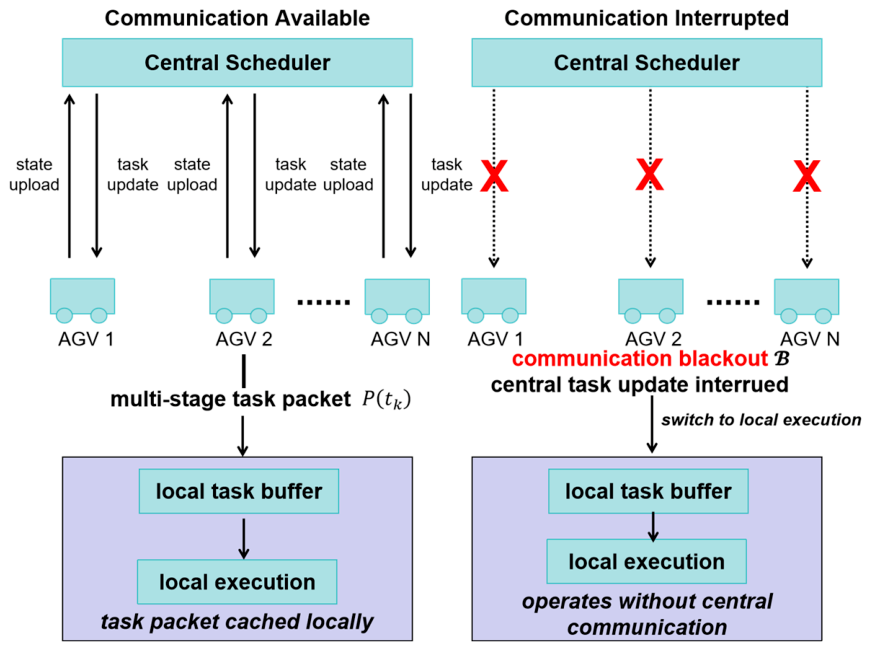
Figure 2.
Overall CAMP framework.
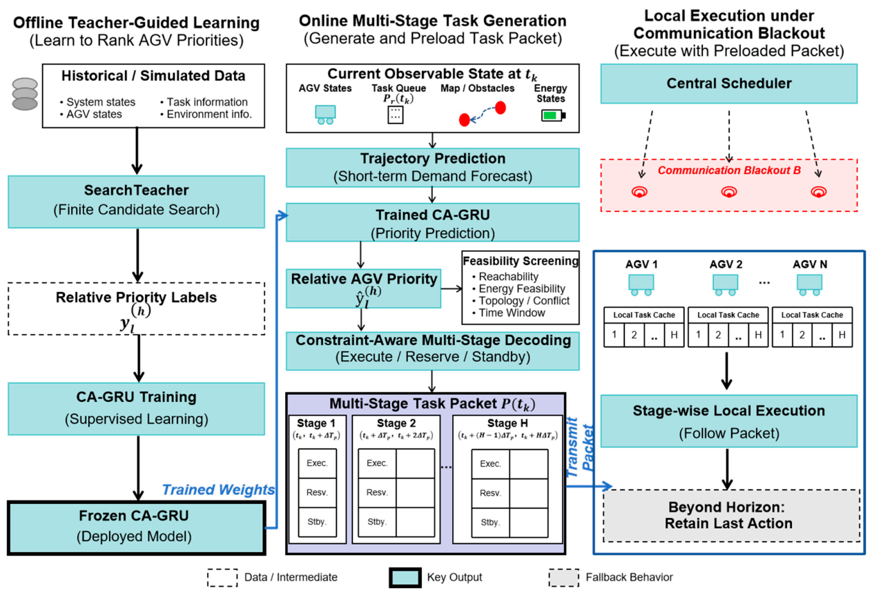
Figure 3.
Multi-stage task preloading and local execution mechanism during communication blackouts.
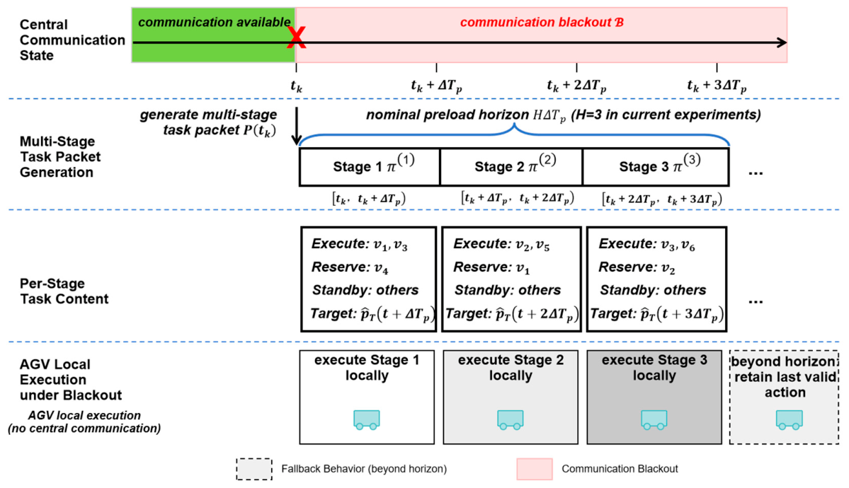
Figure 4.
Baseline spatial configuration of the intelligent-warehouse multi-AGV system and trajectory of the dynamic logistics service demand (model coordinates).
Figure 4.
Baseline spatial configuration of the intelligent-warehouse multi-AGV system and trajectory of the dynamic logistics service demand (model coordinates).
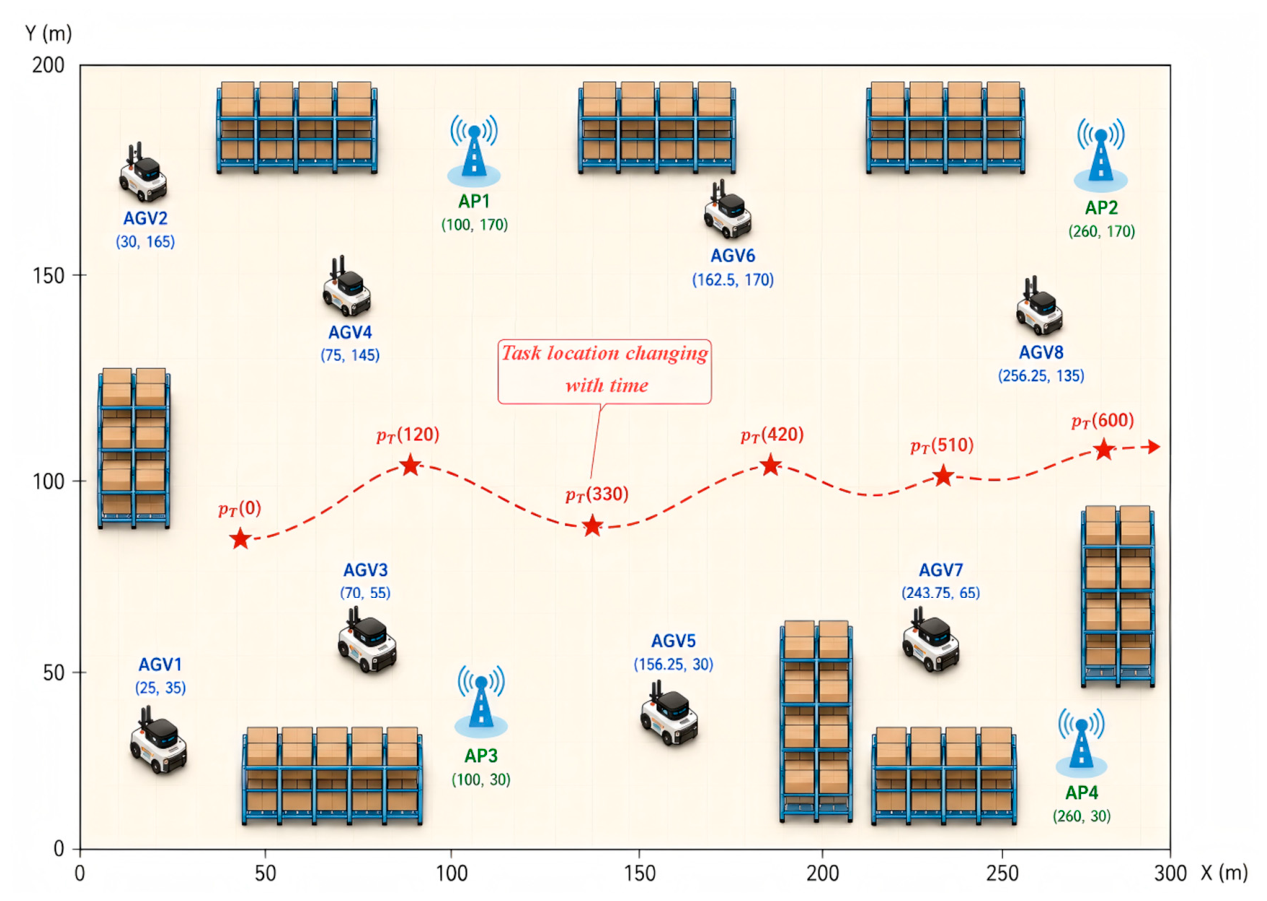
Figure 5.
CA-GRU training convergence and priority-learning performance.
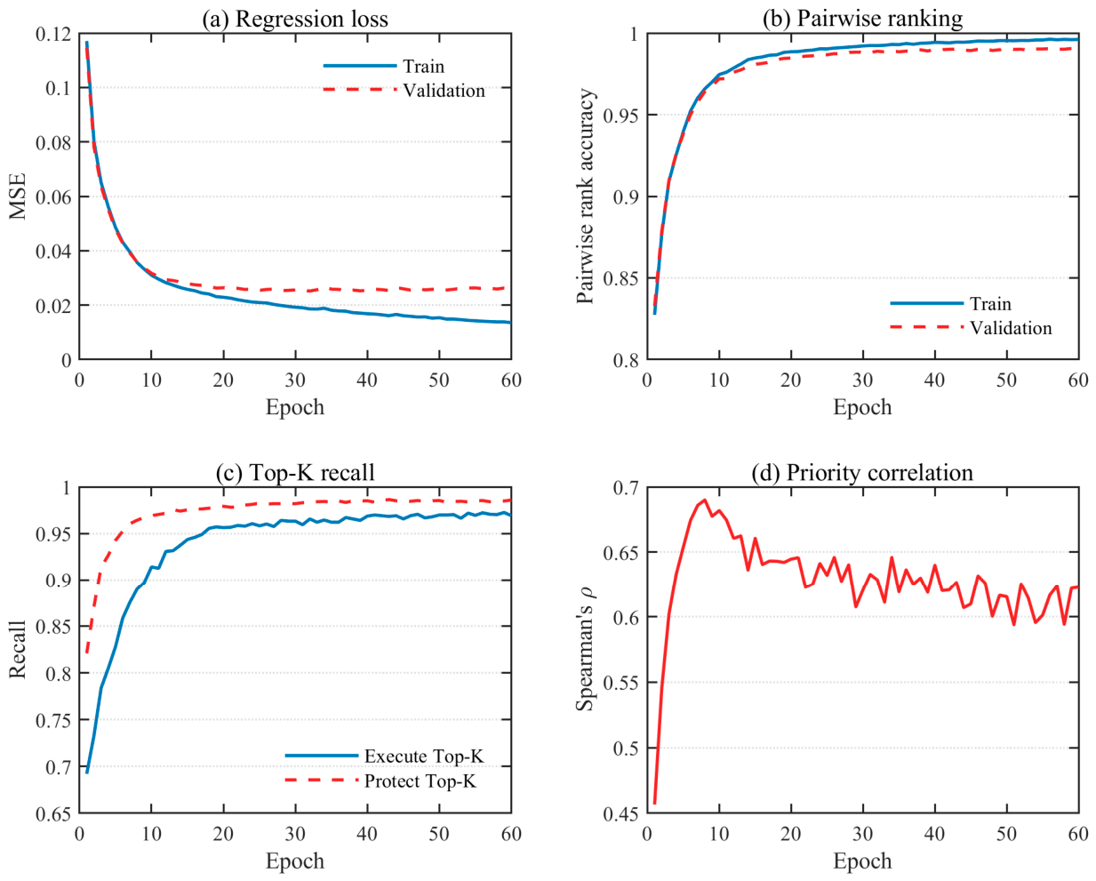
Figure 6.
Effect of the number of preload stages on task-packet coverage and energy consumption.
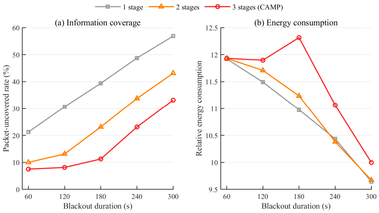
Figure 7.
Core service-continuity performance of the four methods under different communication-blackout durations.
Figure 7.
Core service-continuity performance of the four methods under different communication-blackout durations.
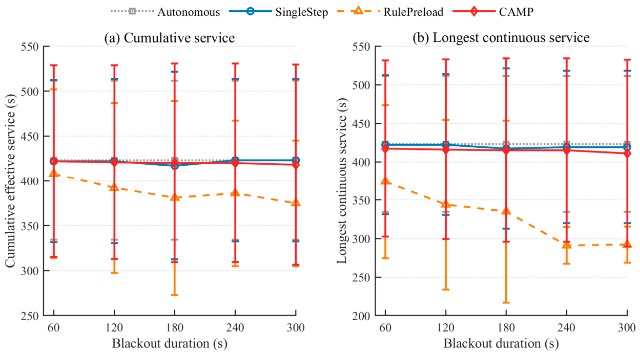
Figure 8.
Comparison of command timeliness and resource efficiency for the four methods.
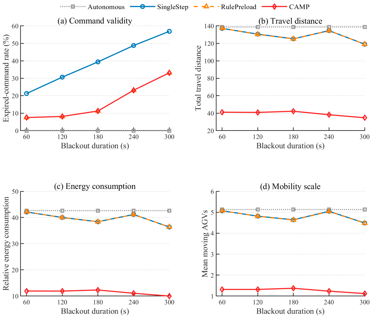
Figure 10.
End-to-end task-packet generation time of SearchTeacher and CAMP.
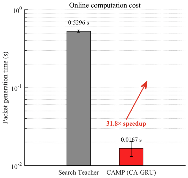
Table 1.
Main experimental and implementation parameters.
| Parameter | Value |
| System setting | 8 AGVs, 4 APs; simulation duration = 600 s; decision interval = 30 s; 30 independent random seeds per configuration |
| Forced-blackout duration | 60, 120, 180, 240, and 300 s |
| CAMP preload and constraints | 3 stages × 60 s = 180 s; maximum 3 Execute and 2 Reserve AGVs; vmax=0.055; service radius = 68–80; coverage margin = 2; minimum authorized energy = 5 |
| Trajectory prediction | 180 s horizon; CV/CT/WA weights = 0.60/0.27/0.13 |
| SearchTeacher candidates | 12 predefined candidates; stage-wise look-ahead distance patterns = ((45,75,150)) and ((75,150,150)) |
| SearchTeacher scoring | Six score weights = 0.38/0.24/0.18/0.10/0.07/0.03; discount factor γ=0.92 |
| CA-GRU configuration | 95-dimensional input; 3-dimensional stage encoding; 64 hidden units; 120 scenarios / 2040 samples |
| CA-GRU training | Adam; learning rate = 1 × 10⁻³; batch size = 16; 60 epochs; maximum gradient norm = 5.0; frozen checkpoint = epoch 56 |
| CA-GRU loss and ranking | Regression/ranking/stage-consistency weights = 4.0/0.75/0.10; ranking threshold (\delta_y=0.30); ranking margin (\delta=0.35) |
| Fallback decoding | Reachability-margin / remaining-energy weights = 0.7/0.3 |
Note: The fixed stage-wise role transitions of RulePreload are not constrained by CAMP’s online-decoding budget of 3 Execute/2 Reserve vehicles; the random seeds used for training and formal evaluation are independent.
Table 2.
Ablation results for the number of preload stages.
| 3-stage relative energy consumption | 2-stage relative energy consumption | 1-stage relative energy consumption | 3-stage task-packet uncovered rate | 2-stage task-packet uncovered rate | 1-stage task-packet uncovered rate | Blackout duration / s |
| 11.93 | 11.93 | 11.92 | 7.50% | 10.00% | 21.25% | 60 |
| 11.90 | 11.71 | 11.49 | 8.12% | 13.12% | 30.63% | 120 |
| 12.32 | 11.23 | 10.98 | 11.25% | 23.12% | 39.38% | 180 |
| 11.06 | 10.38 | 10.44 | 23.12% | 33.75% | 48.75% | 240 |
| 10.00 | 9.67 | 9.64 | 33.12% | 43.12% | 56.88% | 300 |
Note: The uncovered rate is calculated from the discrete AGV–decision-instant samples defined in Equation (28), and relative energy consumption uses a unified model scale. Because deterministic per-vehicle communication windows remain outside the unified forced-blackout interval, the most recent task-packet refresh time may differ among vehicles. The uncovered rate therefore depends jointly on each vehicle’s refresh history, the number of preload stages, and the blackout duration, and cannot be derived simply from the ratio between blackout duration and nominal preload horizon.
Table 3.
Mean system performance of the four methods over five communication-blackout conditions.
| Mean number of moving AGVs | Total relative energy consumption | Total travel distance (model units) | Expired-command rate / % | Longest continuous service / s | Cumulative effective service / s | Method |
| 5.13 | 42.63 | 138.81 | 0.00 | 423.0 | 423.0 | Autonomous |
| 4.81 | 39.60 | 129.30 | 39.38 | 419.8 | 421.4 | SingleStep |
| 4.81 | 39.61 | 129.23 | 16.63 | 327.2 | 388.4 | RulePreload |
| 1.27 | 11.44 | 39.43 | 16.63 | 414.8 | 420.2 | CAMP |
Note: Results are aggregate means over the five blackout conditions. Each condition uses 30 independent random seeds, and methods are compared in pairs under the same random seed. Energy consumption is a relative operating cost on the model scale.
Disclaimer/Publisher’s Note: The statements, opinions and data contained in all publications are solely those of the individual author(s) and contributor(s) and not of MDPI and/or the editor(s). MDPI and/or the editor(s) disclaim responsibility for any injury to people or property resulting from any ideas, methods, instructions or products referred to in the content. |
© 2026 by the authors. Licensee MDPI, Basel, Switzerland. This article is an open access article distributed under the terms and conditions of the Creative Commons Attribution (CC BY) license (http://creativecommons.org/licenses/by/4.0/).
Copyright: This open access article is published under a Creative Commons CC BY 4.0 license, which permit the free download, distribution, and reuse, provided that the author and preprint are cited in any reuse.