

Submitted:
21 October 2026
Posted:
22 October 2026
You are already at the latest version
Abstract
The ionospheric quasi-biennial oscillation (QBO) is the sum of the solar QBO and the terrestrial QBO from below. In the present study, we focus on the QBO modulations of diurnal variations in mesospheric temperature and in the daily range of total electron content (ΔTEC) values at low latitudes. The diurnal tide (DW1) in mesospheric temperature is observed by the Aura Microwave Limb Sounder (Aura/MLS) from 2004 to 2021 and shows a dominant modulation at the QBO period of 28 months. This QBO modulation is transfered into the equatorial ionosphere by diurnal electric currents in the ionospheric dynamo region and the equatorial plasma fountain effect. Thus, the QBO modulation of the ΔTEC variation is partly generated by the terrestrial QBO from below. We decomposed the observed ionospheric QBO in ΔTEC from Global Navigation Satellite System (GNSS) into the terrestrial QBO part (from Aura/MLS) and the solar QBO part where the latter is derived from the QBO modulation of the solar flux at 10.7 cm (F10.7). The magnitude of the terrestrial QBO is 34% of the magnitude of the solar QBO in its effect on diurnal TEC variation. The supercomposition of terrestrial and solar QBO explains 81% of the ionospheric QBO signal in ΔTEC. The correlation between the QBO modulation in ΔTEC and solar flux F10.7 is 0.97. The maximal cross-correlation between the mesospheric QBO modulation in DW1 and the stratospheric QBO modulation in zonal wind is 0.97 with a certain phase lag.
Keywords:
QBO
; tide
; middle atmosphere
; ionosphere
; GNSS
; microwave limb sounder
1. Introduction
The quasi-biennial oscillation (QBO) of zonal wind is strongest in the equatorial stratosphere. The QBO period is around 28 months. The extensive research about the QBO is summarized in the review article of [1]. Today it is accepted that the QBO is the result of nonlinear wave-mean flow interaction, where high-frequency atmospheric waves are propagating upward and deposit their eastward or westward momentum at stratospheric heights leading to the reversal of the zonal wind with a period of about 28 months. The QBO is a vital climate driver because it influences the global ozone distribution, it modulates the stratospheric polar vortex, and the modeling of the QBO is crucial for improvement of long-range weather and seasonal forecasts [1].
An open question is how the stratospheric QBO signal can propagate into the thermosphere and ionosphere. Atmospheric modeling by [2,3] showed that upward wave flux generates a modulation of the amplitude of the diurnal westward propagating tide (DW1) in the mesosphere with the QBO period and interannual changes of the tidal amplitude of about 30%. Satellite observations also found a QBO modulation of the mesospheric DW1 amplitude which is about 3 K for the tidal temperature amplitude [4,5,6]. According to [7], the QBO modulation of the DW1 tide induces a QBO modulation of ionospheric electric currents in the dynamo region. At low magnetic latitudes it can be expected that the QBO modulation of the ionospheric currents induces a QBO modulation of the equatorial plasma fountain which is observable as a QBO modulation of the daily TEC range at low latitudes.
Recently, Singh et al. [8] retrieved the ionospheric QBO by using multi-decadal ionospheric observations of GNSS and ionosondes. Firstly, they determined the residuals of the ionospheric observations without the fluctuations caused by solar variability. The residuals were used to determine the terrestrial QBO in the ionosphere. Singh et al. also argued that the QBO modulation of the DW1 tide brings the QBO signal into the ionosphere. They explained that models show decreased TEC values when the DW1 amplitude is enhanced. The terrestrial QBO amplitude of TEC was up to 4% [8]. Values of about 10% were found by [9] for the terrestrial QBO component in TEC at equatorial latitudes.
Generally, the solar QBO of TEC is stronger than the terrestrial QBO of TEC [8,9]. In the present study, we apply a different approach to characterize the terrestrial and the solar QBO of daily TEC range at low latitudes. It is better to take daily TEC range as study parameter than TEC since the TEC range is more directly connected to the diurnal variations of the mesospheric DW1 tide and their induced electric currents in the ionospheric dynamo region. In addition, the present study performs a multiple linear regression of the QBO modulations of the DW1 amplitude (terrestrial QBO) and the QBO modulation of the F10.7 time series (solar QBO). Thus, we fit both QBOs to the QBO in daily TEC range at the same time which is different to the approach of [8,9] who computed firstly the residuals of TEC (subtracted by the solar variations) and later the terrestrial QBO from the residuals. The present study takes advantage of the mesospheric DW1 tide observations from 2004 to 2021 which are based on temperature measurements of the Microwave Limb Sounder on the Aura satellite (Aura/MLS).
The measurements of TEC and temperature by GNSS and Aura/MLS are described in section 2, as well as the data analysis. The results are presented in section 3 and discussed in section 4. The conclusions are given in section 5.
2. Measurement and Data Analysis
2.1. Aura/MLS
The temperature and geopotential height measurements used in this study were obtained from the Microwave Limb Sounder (MLS) aboard NASA’s Aura satellite, which was launched in 2004 [10]. Aura operates in a Sun-synchronous orbit and initially crossed the equator at approximately 01:45 and 13:45 local solar time (LST). These crossing times are close to midnight and noon. The crossing times have changed only slightly since launch; over the 17-year observation period considered here, their mean values are approximately 01:44 and 13:44 LST.
Version 5 Level 2 MLS retrievals were used throughout the analysis. The data were screened according to the quality-control criteria described by [11]. The profiles considered in this study extend from approximately 15 to 95 km altitude. The estimated uncertainty of the MLS temperature measurements is about 1 K in the stratosphere and approximately 3 K in the mesosphere [12].
For each observation day, zonal-mean temperature profiles were derived over the equatorial region, defined here as 10°S–10°N. Owing to the orbital configuration of Aura, MLS provides sampling of equatorial longitudes at intervals of approximately 24°, corresponding to the longitudinal separation between successive ascending or descending equatorial orbital tracks. Two zonal-mean temperature profiles are therefore obtained each day, corresponding nominally to the morning and afternoon equator-crossing times of 01:45 and 13:45 LST, respectively. The MLS retrievals are provided on pressure levels. Using the corresponding geopotential height profiles, the temperature measurements can be converted from pressure coordinates to altitude coordinates, allowing the zonal-mean temperature to be evaluated as a function of geometric altitude.
The equatorial signature of the migrating diurnal tide with zonal wavenumber one (DW1) in zonal-mean temperature was investigated by Hocke [13], who identified its characteristic nodes and bellies. The focus of the present study is the temporal evolution of the DW1 temperature maximum (belly) near 82 km altitude. To quantify this feature, we define an equatorial DW1 temperature amplitude proxy, , as half of the difference between the zonal-mean temperatures measured at the two Aura equator-crossing times:
Here, is used as a proxy for the amplitude of the mesospheric DW1 temperature perturbation at 82 km. Because the Aura equator-crossing times vary slightly over the satellite mission, the nominal times of 01:45 and 13:45 LST should be understood as approximate values. In particular, the crossing times can differ by about 30 s over the 2004–2021 period, with values of approximately 01:44 and 13:44 LST occurring at some epochs.
2.2. GNSS
Ground stations of the Global Navigation Satellite System (GNSS) receive radio signals transmitted by GNSS satellites. Because ionospheric dispersion depends on frequency, observations at multiple frequencies allow the total electron content (TEC) along the signal path to be derived. The International GNSS Service (IGS) has produced global TEC maps since June 1998, with spatial resolutions of in longitude and in latitude and a temporal resolution of 2 h. The final IGS maps combine TEC estimates from several independent analysis centers using different retrieval procedures [14].
We use IGS TEC data from June 1998 through October 2024. The map generation and error estimation are described by Hernández-Pajares et al. [14]; cross-validation with coincident satellite altimeter observations indicates a relative error below 20%. For each grid point and day, we define the daily TEC range as
We then calculate the arithmetic mean of TEC over magnetic latitudes from S to N. The analysis focuses on the resulting mean daily TEC time series for 2004–2021.
2.3. Solar EUV Proxy
Direct measurements of solar extreme ultraviolet (EUV) radiation with high temporal resolution over long time intervals remain challenging. We therefore use the 10.7-cm solar radio flux (F10.7), a long-term proxy for solar activity and EUV radiation [15]. F10.7 is measured approximately three times around local noon at the Dominion Radio Astrophysical Observatory, British Columbia, corresponding to approximately 20:00 UTC. We use the daily F10.7 values distributed by NASA’s OMNIWeb and assign the measurement time of 20:00 UTC, which is not included in the OMNIWeb data files. The resulting daily time series is bandpass-filtered to extract its quasi-biennial component with a central period of 28 months.
2.4. Data Analysis
A digital non-recursive finite impulse response (FIR) bandpass filter with a Hamming window is applied in the forward and reverse directions to ensure zero-phase filtering. The number of filter coefficients corresponds to a time window three times the central period, providing a rapid response to temporal variations. The cutoff frequencies are at of the central frequency which is at 1/28 months. Further details of the filtering procedure are given by Studer et al. [16].
At each altitude level, we calculate the fast Fourier transform (FFT) spectrum of the complete time series after subtraction of its mean. is the proxy of the DW1 tide in temperature at low latitudes in 82 km height. To increase the frequency sampling density, approximately 17 years of zeros are appended before and after the time series. A Hamming window is applied before zero padding to reduce spectral artifacts. The relative fraction of missing data in the 17-year Aura/MLS record is approximately 1%; these gaps are filled by linear interpolation. The resulting amplitude spectra are calibrated using a synthetic sine wave of known amplitude.
3. Results
The Aura/MLS observations clearly show a QBO modulation of the equatorial mesospheric DW1 temperature amplitude. Figure 1 depicts the FFT spectra of the DW1 amplitude series at different altitudes from the troposphere to the mesosphere and for the time interval from 2004 to 2021. A QBO modulation of at the QBO period of 28 months (indicated by the vertical white dashed line) is obvious at mesospheric heights. Since the amplitude depends on the altitude-dependent phase of the observed DW1 tide, we will focus on the amplitude maximum at 82 km altitude where the DW1 phase is apparently at noon or midnight so that Aura/MLS observes a belly (maximum) of the tide. The FFT spectra also show spectral peaks of the annual, semi-annual, terannual and quartannual modulations of the DW1 amplitude.
In order to see the temporal behaviour of the QBO modulation, we filtered the equatorial series at 82 km altitude with a bandpass at the QBO period of 28 months. Figure 2 shows the series which has an amplitude decrease in the years after 2015. Similarly, we filtered the solar F10.7 series for the QBO period of 28 months. Figure 3 shows the result. The QBO modulation of F10.7 is stronger around the solar maximum in 2012 to 2014. This is in agreement with past observations who found a stronger solar QBO of solar EUV during solar maximum years [8].
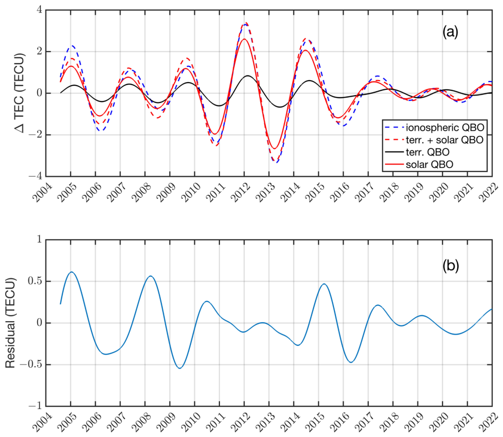
We also filtered the equatorial daily TEC range series (magnetic latitudes from 30°S to 30°N) for the QBO period. The blue dashed line in Figure 4a shows the result which we call here the ionospheric QBO (). The ionospheric QBO has a correlation with the solar QBO of F10.7 from Figure 3 with a correlation coefficient . Thus, the solar QBO of F10.7 or EUV explains a major part of the observed ionospheric QBO of the daily TEC range.
Now, we utilize multiple linear regression in order to interprete the ionospheric QBO as the sum of the solar QBO and the terrestrial QBO:
where a, b, and c are the fitted regression constants. are the residuals of the fit. is the lowpass-filtered F10.7 series (with periods greater than 1 year). is shown in Figure 4a as the red solid line (solar QBO) while is shown as the black solid line (terrestrial QBO). The terrestrial QBO is generated by the multiplication of the mesospheric DW1 amplitude series (filtered at the QBO period) with the low-pass-filtered F10.7 series (periods greater than 1 year). We assume that the terrestrial QBO depends on the strength of the mesospheric tide but also on the strength of the ionization in the dynamo region. The latter is estimated by the F10.7 series where we neglect the high-frequency fluctuations with periods less than 1 year. Finally, Figure 4a shows the fitted sum of the terrestrial and solar QBO as the red dashed line. The residuals of the fit are given by which is shown in Figure 4b. The fit (red dashed line) explains 81% of the observed ionospheric QBO (blue dashed line). For this calculation, we derived the ratio of the sums of the absolute values of both curves. The terrestrial QBO is 34% of the solar QBO contribution to the ionospheric QBO. The correlation between the ionospheric QBO (blue dashed line) and the fit (red dashed line) is 0.98.
The maximum of the cross-correlation between the mesospheric series and the stratospheric QBO (zonal wind series at Singapore at 10 hPa and bandpass-filtered at 28 months) is 0.97. The mesospheric series has further an anti-correlation of with the solar QBO of F10.7.
4. Discussion
The Aura/MLS observations in the equatorial mesosphere clearly show a QBO modulation of the equatorial DW1 temperature amplitude from 2004 to 2021 (Figure 1). This QBO signal of the DW1 tide propagates to the equatorial dynamo region and induces periodic ionospheric electric currents. These currents generate equatorial variations of the daily TEC range via electrodynamical forcing (equatorial plasma fountain) [7]. The QBO-induced ionospheric currents and the induced TEC variations depend on both the magnitude of the DW1 tide and on the magnitude of the ionization. Thus, the contribution of the terrestrial QBO to the ionospheric QBO depends on the product of (variation of mesospheric DW1 tide) and (proxy of the solar EUV-induced photoionization of the ionosphere).
Such a chain of the terrestrial QBO influence on the ionosphere also has been suggested by [8]. The new aspect of the present study is that we use the Aura/MLS observations of the mesospheric DW1 amplitude for the estimation of the associated TEC variation. It is remarkable that the solar QBO and the terrestrial QBO components of the ionospheric QBO interfere in a constructive manner. In case of the terrestrial QBO, a minimum in the DW1 amplitude corresponds to a maximum in the TEC response. In agreement to this observation, Singh et al. [8] explained that atmosphere-ionosphere models show enhanced TEC values when the DW1 amplitude is decreased.
On the other hand, the ionospheric QBO is produced to a major part by the solar QBO in F10.7 (as proxy of the ionizing EUV radiation). Indeed, the correlation between the solar QBO and the ionospheric QBO is 0.97. We utilize the multiple linear regression technique to decompose the ionospheric QBO into the solar QBO and the terrestrial QBO (Figure 4a). We find that the latter two components explain 81% of the observed ionospheric QBO. The terrestrial QBO amounts for 34% of the solar QBO part of the ionospheric QBO. The data analysis of the present study is new since other studies [8,9] subtracted at first the solar variations from the ionospheric TEC before they estimated the terrestrial QBO in TEC. A further new point of the present study is that we analyzed the daily TEC range (instead of TEC). The daily TEC range can be assumed to be more directly influenced by the DW1 tide.
5. Conclusions
The ionospheric QBO reflects the combined contributions of terrestrial forcing from below (terrestrial QBO) and solar EUV forcing (solar QBO). In this study, we investigated QBO-related modulations of diurnal variations in mesospheric temperature and in the daily range of total electron content (TEC) at low latitudes.
The diurnal migrating tide (DW1) in mesospheric temperature, observed by Aura/MLS from 2004 to 2021, exhibits a pronounced QBO modulation with a period of approximately 28 months. This modulation is transmitted to the equatorial ionosphere through tide-induced diurnal electric currents in the ionospheric dynamo region and the equatorial plasma fountain effect. Consequently, the terrestrial QBO signal from the middle atmosphere contributes to the QBO modulation of diurnal TEC variations.
We decomposed the observed ionospheric QBO signal in TEC into terrestrial and solar contributions. The terrestrial component is estimated from the QBO modulation of the mesospheric DW1 tide derived from Aura/MLS observations, while the solar component is inferred from the QBO modulation of the solar radio flux F10.7. Our results show that the terrestrial QBO contribution to diurnal TEC variations has a magnitude equivalent to 34% of the solar QBO contribution. The superposition of the terrestrial and solar components accounts for 81% of the observed ionospheric QBO signal in TEC. Furthermore, the QBO modulation of TEC exhibits a correlation of 0.97 with the solar radio flux F10.7. The mesospheric QBO modulation of DW1 shows a maximum cross-correlation of 0.97 with the stratospheric QBO modulation in zonal wind above Singapore, subject to a phase lag.
The transfer of the terrestrial QBO signal to the ionosphere is still an open question. The present study supported the view that the QBO signal in the mesospheric DW1 tide plays a crucial role. We also quantified the contributions of the terrestrial QBO and solar QBO to the ionospheric QBO.
Author Contributions
Conceptualization, K.H., G.M. and W.W.; methodology, K.H., G.M. and W.W.; software, K.H. and G.M.; validation, K.H. and W.W.; formal analysis, K.H. and W.W.; writing—original draft preparation, K.H.; writing—review and editing, K.H., G.M. and W.W.. All authors have read and agreed to the published version of the manuscript.
Funding
Funding for open-access publication was provided by the University of Bern.
Institutional Review Board Statement
Not applicable.
Informed Consent Statement
Not applicable.
Data Availability Statement
The Aura/MLS data are available from the Aura Validation Data Center (AVDC) at https://avdc.gsfc.nasa.gov/ (accessed on 20 January 2026). The stratospheric zonal wind data over Singapore are provided by NOAA at https://www.cpc.ncep.noaa.gov/data/indices/ (accessed on 1 October 2026). The F10.7 data are provided by NASA’s Omniweb (https://omniweb.gsfc.nasa.gov/ (accessed on 1 October 2026).
Acknowledgments
We thank the Aura/MLS team for the high quality data. We also thank the reviewers and the editor for their work and improvements.
Conflicts of Interest
The authors declare no conflicts of interest.
References
- Baldwin, M.P.; Gray, L.J.; Dunkerton, T.J.; Hamilton, K.; Haynes, P.H.; Randel, W.J.; Holton, J.R.; Alexander, M.J.; Hirota, I.; Horinouchi, T.; et al. The quasi-biennial oscillation. Rev. Geophys. 2001, 39, 179–229. [Google Scholar] [CrossRef]
- Hagan, M.E.; Burrage, M.D.; Forbes, J.M.; Hackney, J.; Randel, W.J.; Zhang, X. QBO effects on the diurnal tide in the upper atmosphere. Earth Planets Space 1999, 51, 571–578. [Google Scholar] [CrossRef]
- Mayr, H.G.; Mengel, J.G. Interannual variations of the diurnal tide in the mesosphere generated by the quasi-biennial oscillation. J. Geophys. Res. Atmos. 2005, 110. [Google Scholar] [CrossRef]
- Wang, J.C.; Tsai-Lin, R.; Chang, L.C.; Wu, Q.; Lin, C.C.; Yue, J. Modeling study of the ionospheric responses to the quasi-biennial oscillations of the sun and stratosphere. J. Atmos. Sol.-Terr. Phys.;Vert. Coupling Atmos.-Ionos. Syst. Recent Prog. 2018, 171, 119–130. [Google Scholar] [CrossRef]
- Burrage, M.D.; Hagan, M.E.; Skinner, W.R.; Wu, D.L.; Hays, P.B. Long-term variability in the solar diurnal tide observed by HRDI and simulated by the GSWM. Geophys. Res. Lett. 1995, 22, 2641–2644. [Google Scholar] [CrossRef]
- Niciejewski, R.; Wu, Q.; Skinner, W.; Gell, D.; Cooper, M.; Marshall, A.; Killeen, T.; Solomon, S.; Ortland, D. TIMED Doppler Interferometer on the Thermosphere Ionosphere Mesosphere Energetics and Dynamics satellite: Data product overview. J. Geophys. Res. Space Phys. 2006, 111. [Google Scholar] [CrossRef]
- Yamazaki, Y.; Liu, H.; Sun, Y.Y.; Miyoshi, Y.; Kosch, M.J.; Mlynczak, M.G. Quasi-biennial oscillation of the ionospheric wind dynamo. J. Geophys. Res. Space Phys. 2017, 122, 3553–3569. [Google Scholar] [CrossRef]
- Singh, D.; Goncharenko, L.P.; Zhang, S.R. Imprint of the Quasi-Biennial Oscillation on the Ionosphere and Thermosphere. J. Geophys. Res. Space Phys. 2026, 131, e2025JA034748. [Google Scholar] [CrossRef]
- Tang, W.; Xue, X.H.; Lei, J.; Dou, X.K. Ionospheric quasi-biennial oscillation in global TEC observations. J. Atmos. Sol.-Terr. Phys. 2014, 107, 36–41. [Google Scholar] [CrossRef]
- Waters, J.; Froidevaux, L.; Harwood, R.; Jarnot, R.; Pickett, H.; Read, W.; Siegel, P.; Cofield, R.; Filipiak, M.; Flower, D.; et al. The Earth observing system microwave limb sounder (EOS MLS) on the aura Satellite. IEEE Trans. Geosci. Remote Sens. 2006, 44, 1075–1092. [Google Scholar] [CrossRef]
- Livesey, N.J.; Read, W.G.; Wagner, P.A.; Froidevaux, L.; Santee, M.L.; Schwartz, M.J.; Lambert, A.; Valle, L.F.M.; Pumphrey, H.C.; Manney, G.L.; et al. Earth Observing System (EOS) Aura Microwave Limb Sounder (MLS) Version 5.0x Level 2 and 3 data quality and description document. JPL D-105336 Rev. B. 2022. Available online: https://mls.jpl.nasa.gov/data/v5-0_data_quality_document.pdf.
- Schwartz, M.J.; Lambert, A.; Manney, G.L.; Read, W.G.; Livesey, N.J.; Froidevaux, L.; Ao, C.O.; Bernath, P.F.; Boone, C.D.; Cofield, R.E.; et al. Validation of the Aura Microwave Limb Sounder temperature and geopotential height measurements. J. Geophys. Res. Atmos. 2008, 113, D15S11. [Google Scholar] [CrossRef]
- Hocke, K. Influence of Sudden Stratospheric Warmings on the Migrating Diurnal Tide in the Equatorial Middle Atmosphere Observed by Aura/Microwave Limb Sounder. Atmosphere 2023, 14. [Google Scholar] [CrossRef]
- Hernández-Pajares, M.; Juan, J.M.; Sanz, J.; Orus, R.; Garcia-Rigo, A.; Feltens, J.; Komjathy, A.; Schaer, S.C.; Krankowski, A. The IGS VTEC maps: a reliable source of ionospheric information since 1998. J. Geod. 2009, 83, 263–275. [Google Scholar] [CrossRef]
- Tapping, K.F. The 10.7 cm solar radio flux (F10.7). Space Weather 2013, 11, 394–406. [Google Scholar] [CrossRef]
- Studer, S.; Hocke, K.; Kämpfer, N. Intraseasonal oscillations of stratospheric ozone above Switzerland. J. Atmos. Sol.-Terr. Phys. 2012, 74, 189–198. [Google Scholar] [CrossRef]
Figure 1.
FFT spectra of the time series of DW1 temperature amplitude at the equator (10°S to 10°N) at different altitudes, based on Aura/MLS observations from 2004 to 2021. The frequency of the QBO (1/(28 months)) is denoted by the vertical white dashed line.
Figure 1.
FFT spectra of the time series of DW1 temperature amplitude at the equator (10°S to 10°N) at different altitudes, based on Aura/MLS observations from 2004 to 2021. The frequency of the QBO (1/(28 months)) is denoted by the vertical white dashed line.
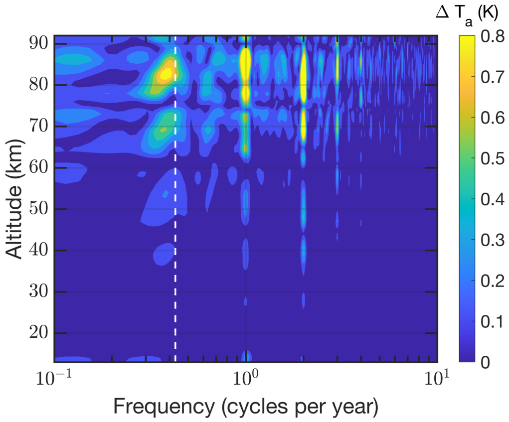
Figure 2.
Time series of the bandpass-filtered, equatorial DW1 temperature amplitude at 82 km height. The bandpass is taken at a period of 28 months of the QBO.
Figure 2.
Time series of the bandpass-filtered, equatorial DW1 temperature amplitude at 82 km height. The bandpass is taken at a period of 28 months of the QBO.
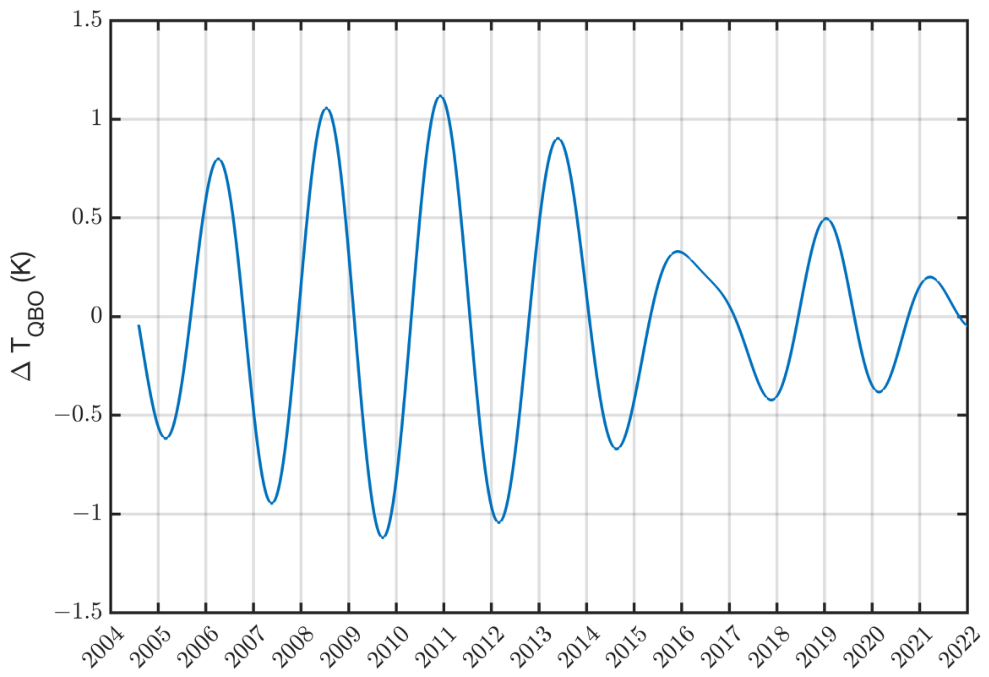
Figure 3.
Time series of the bandpass-filtered solar flux F10.7. The bandpass is taken at a period of 28 months of the QBO.
Figure 3.
Time series of the bandpass-filtered solar flux F10.7. The bandpass is taken at a period of 28 months of the QBO.
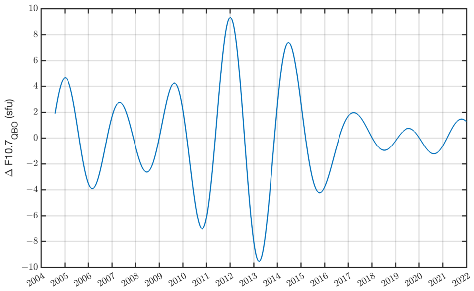
Figure 4.
(a) The time series of the QBO-bandpass-filtered daily TEC range (magnetic latitudes from 30°S to 30°N) is shown by the blue dashed line. The fit obtained by multilinear regresssion is shown by the red dashed line which is the sum of the solar QBO component (red line) and the terrestrial QBO component (black line). The bandpass is always taken at a period of 28 months of the QBO. (b) Difference between the blue dashed line and the red dashed line giving the residual series.
Disclaimer/Publisher’s Note: The statements, opinions and data contained in all publications are solely those of the individual author(s) and contributor(s) and not of MDPI and/or the editor(s). MDPI and/or the editor(s) disclaim responsibility for any injury to people or property resulting from any ideas, methods, instructions or products referred to in the content. |
© 2026 by the authors. Licensee MDPI, Basel, Switzerland. This article is an open access article distributed under the terms and conditions of the Creative Commons Attribution (CC BY) license.
Copyright: This open access article is published under a Creative Commons CC BY 4.0 license, which permit the free download, distribution, and reuse, provided that the author and preprint are cited in any reuse.