

Submitted:
21 October 2026
Posted:
21 October 2026
You are already at the latest version
Abstract
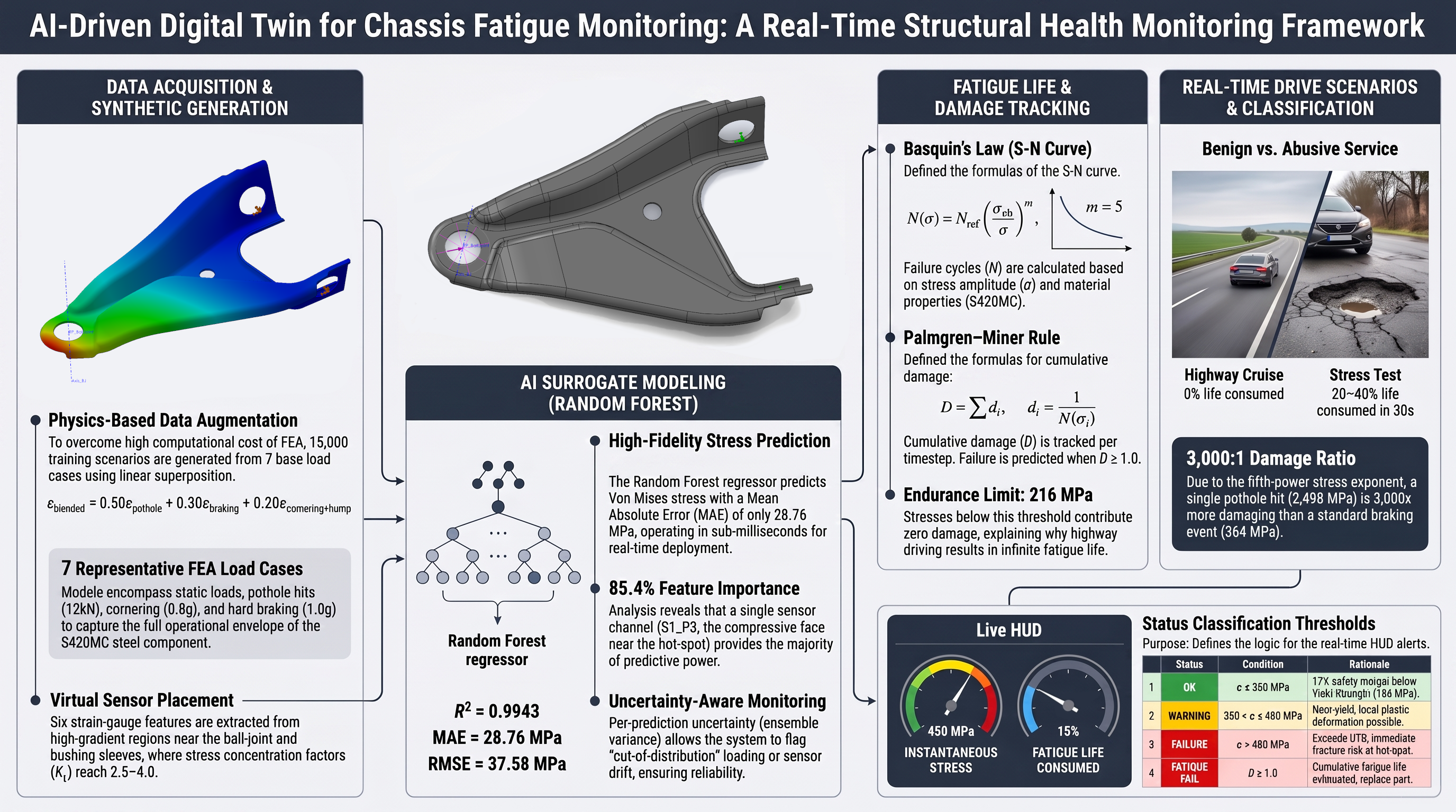
The paper presents a new Integrated Framework for AI predictive Maintenance (AMIFAIM - Andrei Muresan Integrated Framework for AI predictive Maintenance), which allows an online monitoring of the main components fatigue life. A Random Forest regressor, trained on 15,000 synthetic loading scenarios generated by physics-based superposition of seven finite element load cases, serves as a real-time surrogate for structural simulation. The framework is demonstrated on a lower control arm made from S420MC steel (EN 10149-2) in a Dacia Logan front suspension. The trained model predicts Von Mises stress from six strain-gauge channels with R² = 0.9943, MAE = 28.76 MPa, and RMSE = 37.58 MPa on unseen test data, while providing uncertainty estimates per-prediction from the variance of the ensemble. Cumulative fatigue damage is tracked in real time using the Palmgren–Miner rule with an S-N curve calibrated for hot-spot stress conditions. Simulated drive scenarios confirm that the system correctly distinguishes between benign service (near-zero fatigue damage under highway loading) and abusive conditions (5–8% life consumption in 30 seconds under repeated impact loading), consistent with the expected behavior of a properly designed suspension link. The entire pipeline – data augmentation, training, prediction, fatigue tracking, and visualization—is driven by a single configuration file. Applying it to a new component requires only finite element results and material properties; no software changes are needed. The framework is designed to be reconfigured for components for which representative FEA load cases and material-fatigue inputs are available. The current implementation operates on FEA-derived virtual sensor data, with the architecture designed for direct replacement by physical strain-gauge hardware in future experimental validation.
Keywords:
digital twin
; structural health monitoring
; Random Forest
; fatigue life prediction
; automotive chassis
; finite element analysis
; lower control arm
1. Introduction
Evolution of the automotive industry over the past years increased the demand for lightweight, high-performance chassis structures, and thus issues regarding structural integrity started to be more in discussion.
Current maintenance strategies for automotive components are usually either a scheduled inspection strategy, where at a certain number of kilometers the vehicle is taken in for inspection of certain components, or a run-to-failure strategy, where the vehicle is used until certain components break and are then replaced, as opposed to condition-based and predictive approaches.
The aim of this paper is to demonstrate that a digital twin concept that simulates real-time structural monitoring and predictive maintenance can be created, and that this can serve as a guideline to be adapted to any structural component.
The major gap in the literature that this paper aims to fill is the fact that most digital twin research focuses on aerospace or large civil structures; automotive chassis, especially stamped steel suspension parts, are underrepresented.
This paper provides the necessary methodology and guideline on how a predictive maintenance digital twin can be implemented for almost any structural part.
2. Literature Review
2.1. Digital Twins in Structural Health Monitoring
A digital twin as a three-component system was introduced by Grieves and Vickers [1]. The first component is a physical asset; the second one is the virtual replica (containing all information related to the physical asset) while the third is a bi-directional data link which connects them. Physical parts send sensor information to the virtual model which in turn sends predictions and warning back, thus the component in use is continuously compared to its physical counterpart.
Further research into machine learning integration with structural health monitoring was done by Malekloo et al. [2], which identified four emerging technologies – UAV-based inspection, mobile device sensor networks, augmented reality for field visualization, and digital twins with physics-guided machine learning. They also noted that many SHM systems remain reactive, detecting damage only after it has occurred. Another issue that needs tackling is data scarcity, which is a primary barrier to deployment of structural monitoring systems, identified by Jia and Li [3].
Ammar [4] proposed a digital twin for real-time condition monitoring and remaining-life prediction and demonstrated it on the coil springs of a passenger-car suspension. Eddy et al. [5] demonstrated predictive maintenance on a military ground vehicle using a digital twin framework but relied on statistical signal features and condition indicators rather than component-level stress. Qiu et al. [6] adapted a digital twin framework for adaptive suspension control, which is closer to the present goal but aimed at ride comfort rather than stress prediction.
Lai et al. [7] built a digital twin for an aircraft wing that combines computational (FEA-based) data with strain-gauge measurements for load identification and fatigue damage estimation. This represents the state of the art for physics-based, live-sensor, continuously updated systems—but nothing comparable has been developed for the automotive chassis. Existing automotive digital twins monitor the vehicle as a system; the present work targets the fatigue life of individual structural parts.
2.2. Machine Learning for Stress Prediction
A single FEA simulation of the lower control arm (LCA) takes minutes on a desktop workstation. For design iteration that is acceptable; for real-time monitoring at 2 Hz, it is not, a prediction is required every 500 ms. A practical solution is to train the machine learning model offline on the FEA results and deploy it as a surrogate that would produce an adequate answer in milliseconds. The trade-off is accuracy: the surrogate is an approximation.
Liang et al. [8] demonstrated one of the earliest FEA-to-digital-twin surrogates—a neural network that predicted aortic wall stress distributions from patient geometry. Yang et al. [9] extended this to hierarchical composites using a conditional generative adversarial network that predicts full stress and strain tensor fields directly from microstructure images. Maurizi et al. [10] used graph neural networks operating directly on the FE mesh. Shao et al. [11] and Sheen and Nowell [12] further demonstrated deep-learning surrogates for parametric stress analysis enabling rapid “what-if” studies.
Vurtur Badarinath et al. [13] reviewed machine learning approaches as FEA surrogates, which confirms that this method performs reliably for one-dimensional structural systems with limited data available.
For this study, because of the initial data used and the predictions needed, a Random Forest Regressor was chosen. This type of machine learning model has three distinct properties that make it suitable in this study:
- Built-in prediction uncertainty. Mentch and Hooker [14] showed that Random Forest predictions are asymptotically normal when trees are built on subsamples, enabling confidence intervals at no additional computational cost. Shaker and Hüllermeier [15] further distinguished between aleatoric uncertainty (irreducible sensor noise) and epistemic uncertainty (lack of training data in a region of the input space).
- Feature importance. The Random Forest automatically ranks which strain-gauge channels contribute most to stress prediction, which is useful for sensor placement optimization.
- Robustness with limited data. Breiman [16] showed that random forests, which combine bootstrap aggregation (bagging) of decision trees with random feature selection, have a generalization error that converges as trees are added and are robust to noise. With 12,000 training points and only six features, overfitting risk is minimal.
The trade-off is that the Random Forest cannot extrapolate—it can only predict within the envelope of its training data.
2.3. Fatigue Life Estimation
Fatigue design of metallic structures rests on the S-N curve (stress vs. number of cycles to failure) and a damage accumulation rule. Lazovic et al. [17] traced the century-long development of Palmgren’s 1924 bearing-life formula up to the current ISO 281 standard; Palmgren’s linear damage hypothesis was formalized by Miner in 1945 [18] and is implemented in modern design standards such as Eurocode 3 [19]. Miner’s rule states that each stress cycle consumes a fraction 1/N(σ) of the component’s life and failure occurs when the sum of these fractions reaches 1.0. Despite known limitations, Palmgren–Miner remains the standard in automotive chassis design.
The fatigue limit of steel is governed by the size and location of the most critical defect, as shown by Murakami et al. [20], who estimate the fatigue limit from the material hardness (σw ≈ 1.6 HV). For structural steels such as S420MC, the endurance limit is commonly taken as 40–50% of the ultimate tensile strength. This was extended to corroded members and joints of steel structures by Adasooriya et al. [21], who proposed an S-N formula for corroded steel details derived from corrosion-fatigue tests in air, fresh water and seawater—relevant for future iterations because the LCA is exposed to road salt. Savaidis and Vormwald [22] showed, for welded joints of city-bus floor structures, that hot-spot stresses computed by FEA identify the failure-critical locations and, combined with the IIW hot-spot approach, give accurate fatigue-life estimates; this hot-spot principle underlies the Nref calibration approach used here.
Linear damage accumulation according to Palmgren–Miner remains a practical engineering tool: Weber et al. [23] used it to derive a complete S-N curve from a single load-increase test. This is relevant because in our study the LCA encounters variable stress as the vehicle travels in different road conditions. Naik et al. [24] performed multi-body dynamics simulation coupled with fatigue analysis on an all-terrain vehicle LCA and found the twist load event to be the most damaging. Abebe and Koo [25] quantified uncertainty in LCA fatigue life predictions using probabilistic methods; in the present system, prediction uncertainty is provided by the Random Forest ensemble.
Wu and Wang [26] predicted the fatigue life of a suspension lower control arm and extended it using surface-bonded and embedded piezoelectric elements, Gao et al. [27] developed an embedded sensor for real-time, in-situ fatigue life monitoring, and Lagerblad et al. [28] combined FE modelling with vibration measurements for strain-based fatigue prediction.
2.4. Data Augmentation for Small FEA Datasets
Machine learning models need data. The FEA analysis produced seven load cases, a number dictated by engineering judgement and computational budget, not by machine learning requirements. Running 15,000 FEA simulations to train the model would take weeks of computational time and is impractical for a methodology intended to be deployed on any component with minimal setup.
Kim and Shin [29] developed a deep-learning framework for multi-scale FEA that incorporated data augmentation to overcome limited training data. Augmentation respecting the underlying physics produces physically plausible training samples. Admasu et al. [30] reinforced this with a physics-informed variational autoencoder that generated synthetic structural data while enforcing constitutive constraints.
In this study the principle of superposition validated by Bagathi et al. [31] for linear FEA is used. They demonstrated that for linear-elastic analysis the stress field under a combined load equals the sum of the stress fields under each load applied independently, with less than 0.1% error relative to a direct FEA solution, validating this approach for the linear elastic regime. The blending procedure—three anchor cases, normalized weights summing to 1, and 2% Gaussian noise—exploits this exactness for the strain channels while accepting a conservative approximation for the Von Mises scalar. The result is 15,000 physically plausible training scenarios from seven FEA runs, with full traceability to the original load cases.
The studies reviewed above address individual components of a structural health monitoring pipeline — surrogate modelling, fatigue accumulation, data augmentation, or sensor-based monitoring — but none combine them into a single, reusable tool. The goal of the present work is to integrate these established methods into a unified framework (AMIFAIM) that can be configured for any structural component and deployed for real-time fatigue life tracking with minimal setup.
3. Methodology
3.1. System Architecture
We define a methodology to create a digital twin concept for predictive maintenance. The framework begins by defining a set of FEA results obtained by running FEA analysis with virtual sensors placed on the selected part. For the automotive context, FEA is run in seven distinct load cases mimicking a driving sequence, as listed in Table 1.
Because only seven load cases are available, physics-based augmentation is used to obtain 15,000 synthetic load cases (12,000 for training and 3,000 for testing), which is sufficient to train a Random Forest Regressor. The trained regressor approximates the FEA results on unseen test data with R² = 0.994 (Section 4.1). All real-time data is used to calculate component fatigue over time and visualized in an HTML dashboard (Figure 1 and Figure 2).
This architecture was chosen primarily because it is simple, easy to reproduce, and can run on a laptop with no proprietary dependencies other than a SolidWorks license. All component-specific data—FEA results, material properties, fatigue constants, and classification thresholds—resides in a single configuration file. Switching to a different component therefore requires only editing the configuration file and retraining the Random Forest Regressor; no changes to the software itself are needed. The novelty of the AMIFAIM framework is that it combines knowledge from existing studies, and tries to fill in the gaps left by these studies, defining 5 separate applications which have been integrated within the functional pipeline of the predictive maintenance system:
- config.py - Single Source of Truth - Contains reference FEA load cases, material properties, fatigue S-N curve parameters, stress classification thresholds, 5 drive scenario sequence. Written in Python because it is better for scientific data structures, it is a shared import for all scripts, it can use NumPy (mathematical functions) and Pandas (data analysis) ecosystems.
- Training_Model.py - AI Training Pipeline - The main function of this application is to blend reference FEA cases to obtain synthetic data, add gaussian noise, train random forest regressor and cross validate results, save model *.pkl files and graphs. Written in Python because of the availability of scikit-learn to train AI, Pandas for data analysis, matplotlib for graph publication.
- Simulation_Drive.py - Real Time Simulation Engine - the main function for this application is to pick test samples that match the drive scenario, add sensor drift, AI prediction of stress and classification according to OK / WARNING / FAILURE / FATIGUE FAIL, accumulates Palmgren-Miner fatigue damage. Written in Python because it can load .pkl model files directly and use NumPy for real time computation.
- server.py - HTTP Server & Process Coordinator - serves the dashboard and uses 6 api endpoints to deliver data to the dashboard. “/api/start” - launches simulation, “/api/train” - launches training, “/api/status, /api/train-status, /api/scenarios” - lists drive scenarios, “/api/part” - list of structural parts. This application also launches “Training_Model.py” and “Simulation_Drive.py” as independent sub-processes. Written in Python because of the built-in server module, and it’s the same interpreter used for Machine Learning scripts.
- dashboard.html - Browser Dashboard - displays a 2D car scene that reacts to road events, displays a FEA mesh for stress color mapping, or text only for OK / WARNING / FAILURE, these 3 scenes can be changed at any time. Vanilla Javascript for HUD panels and fatigue gauge, fetch API which polls live_data.json at 10 Hz.
The output of the AMIFAIM pipeline is a series of files that are proof that the system is working (Figure 3)
- partname_AI_Model.pkl - serialized random forest trees for each defined part;
- partname_Test_Data.pkl - 3000 hold-out test scenarios;
- training_metric.json - R², RMSE, MAE and Cross Validation Scores;
- partname_Feature_Names.pkl - ordered list of 6 sensor columns;
- Augmented_Data_15k.csv - 15,000 training dataset (synthetic data);
- 4 validation graphs in PNG format - present further in this study;
- live_data.json - real-time IPC bridge (polled by Dashboard at 10Hz);
- Simulation_Results_Log.csv - full session log;
- Simulation_Report.html - self-contained report created using Chart.js.
3.2. Study Component and Material
3.2.1. Component Description
This new AMIFAIM methodology has been tested onto a particular case study, the lower control arm of the Dacia Logan vehicle. The lower control arm (LCA) is a forged or stamped-steel suspension link that connects the wheel hub/knuckle to the vehicle sub-frame. It is the lowest and most heavily loaded link in a MacPherson strut or double-wishbone front suspension. The LCA typically has a triangular (A-shaped) planform with two widely spaced bushing connections at the sub-frame end and a single ball joint at the outboard end.
Wheel location and guidance. The LCA constrains the wheel’s lateral and longitudinal position relative to the body while allowing vertical travel. In a MacPherson strut layout, the LCA is the sole lower locating member—it defines the lower pivot axis of the suspension and directly controls the wheel’s camber change during compression.
Multi-axial load transfer. The LCA transmits all ground-contact forces from the tire contact patch upward into the sub-frame: vertical loads (vehicle weight, pothole impacts up to 3–4× static load), lateral loads (cornering forces up to 1.0–1.2 g), and longitudinal loads (braking and acceleration). These loads arrive simultaneously and at varying ratios, creating a complex multi-axial stress state that makes fatigue the governing failure mode.
Stress concentration locations. The ball-joint bore, the bushing pressed-in sleeves, and the stamped transition fillets are the critical fatigue locations. FEA typically shows stress concentration factors Kₜ of 2.5–4.0 at these features, meaning local peak stresses can be several times higher than the nominal arm stress.
3.2.2. Material Properties
S420MC hot-rolled micro alloyed steel (EN 10149-2:2013) is selected for the LCA because the component’s compact geometry and high local stresses demand a minimum yield strength of 420 MPa. The higher strength allows thinner gauge material (typically 3–5 mm), which keeps the component weight low. S420MC retains sufficient elongation (≥ 16%) for the deep-drawing and flanging operations needed to form the arm’s complex 3D profile, and its weldability permits robotic MIG/MAG joining of reinforcement brackets at the ball-joint housing. The relevant mechanical and chemical properties are summarized in Table 2.
Because of the LCA design and functionality, special attention must be paid to the ball-joint and bushing interfaces; virtual sensors are placed in those areas. The LCA is an adequate study component because it experiences multi-axial loading, severe stress concentrations at the ball-joint bore and bushing sleeves, and fatigue is the documented failure mode [24,25].
3.3. Finite Element Analysis
Seven static structural load cases were analyzed in SolidWorks Simulation to characterize the LCA’s response across its operational loading envelope. Force magnitudes were derived from vehicle dynamics calculations based on the Dacia Logan’s specifications: kerb mass 1,090 kg, laden mass approximately 1,240 kg, front axle load share ≈ 60% in static conditions, giving a static wheel load of approximately 3,650 N.
Vertical forces were calculated by applying dynamic load factors to the static wheel load: a mild bump (factor ≈ 1.6) gives 6,000 N; a moderate bump at speed (factor ≈ 2.2) gives 8,000 N; a severe pothole or kerb strike (factor ≈ 3.3) gives 12,000 N. These factors are consistent with standard automotive chassis design practice for European road conditions.
The lateral cornering force was derived from the vehicle’s skid pad performance of approximately 0.8 g:
The longitudinal braking force assumed 1.0 g deceleration with forward weight transfer increasing the front share to approximately 73%:
The seven load cases comprise four single-axis cases (two vertical levels, lateral cornering, longitudinal braking), two two-axis combinations, and one three-axis worst case; in the combined cases (LC6, LC7) the longitudinal component was set to 4,000 N. The complete load matrix is presented in Table 3.
The combined cases are necessary because, although the stress tensors superpose linearly, the Von Mises equivalent stress does not: it is a norm of the stress tensor, so VM(A + B) ≤ VM(A) + VM(B), and the location of the peak can shift between load cases. LC7 (three-axis) produces slightly less stress than LC6 (two-axis) because the added lateral force redirects part of the bending stress into membrane stress at the critical cross-section—a geometry-specific interaction that hand calculations would not capture.
LC3 (pure cornering) produces only 103 MPa, far below the other cases. The LCA’s triangular planform is geometrically stiff in the lateral direction, resisting cornering forces through efficient membrane action rather than bending. Fatigue damage is therefore governed almost entirely by vertical loading events.
Forces were applied as distributed loads on the ball-joint bore surface; both bushing bores were constrained with zero displacement (Figure 4). The material was defined as S420MC steel (E = 210 GPa, ν = 0.3) with linear-elastic behavior. The mesh used curvature-based refinement to resolve stress gradients at fillets and bore radii.
Three strain-gauge locations were selected at high-gradient, physically accessible regions of the LCA surface. At each location, two values were extracted: the first principal strain (ε₁, tensile) and the third principal strain (ε₃, compressive), yielding six input features per load case. The target variable is the maximum Von Mises stress, occurring at the ball-joint fillet or bushing sleeve radius. Strain values are stored as dimensionless ratios and converted to microstrain (× 10^6) before model input, matching the output format of physical data acquisition hardware.
3.4. Synthetic Data Generation
For a linear-elastic material like S420MC steel, the principle of superposition holds. If load case A produces a strain εA and load case B produces a strain εB, then applying both simultaneously produces εA+ εB. This is exact for strains (Hooke’s law). For Von Mises stress scalars, it is an approximation because Von Mises is a non-linear function of the stress tensor, but it is a conservative overestimate—the safe side for structural design.
In real-world driving a suspension LCA rarely experiences a single pure load case. The blending procedure works as follows: three of the seven load cases are selected—for example LC2 (pothole), LC4 (hard braking), and LC5 (cornering + bump)—and each is assigned a weight (e.g. 50% pothole, 30% braking, 20% cornering + bump). The resulting strain at each gauge location is:
The weights always sum to one, ensuring every synthetic scenario is an interpolation within the envelope of known FEA results—never an extrapolation beyond it. Because the weights sum to one, a blend represents a scaled mixture of the anchor load states (for example, half of a pothole event plus half of a braking event) rather than their full simultaneous application; full simultaneous combinations are represented by the combined FEA cases LC5–LC7. Three cases are chosen for blending because a two-case blend represents a line in loading space whereas a three-case blend represents a plane, producing much richer combinations.
Gaussian noise (σ = 2%) is added to each strain channel to represent real-world sensor imperfections including electrical noise from the Wheatstone bridge excitation, thermal drift, adhesive creep, and analogue-to-digital quantization error. The same 2% noise is also applied to the blended target stress.
Strictly speaking, superposition applies to the full stress tensor, not to the Von Mises equivalent stress. Scalar superposition of Von Mises values is the standard engineering approximation when the full tensor is not available (SolidWorks exports the scalar maximum, not the tensor at every node); it tends to overestimate the combined stress, making it conservative for structural safety assessment. This is noted as a limitation in Section 4.6 [31].
The output of this procedure is 15,000 synthetic load cases, each containing six strain-gauge readings and the corresponding Von Mises stress, split 80/20: 12,000 for training and 3,000 held out as an unseen test set. The entire dataset is saved as a CSV file for traceability and reproducibility.
3.5. Machine Learning Model
3.5.1. Random Forest Regressor
The Random Forest Regressor operates by building 100 independent decision trees, each making its own stress estimate based on the same six strain-gauge readings. Each tree has been trained on a slightly different subset of the 12,000 training scenarios and has developed its own internal decision rules, for example: if S1_P3 < −2,500 με, the stress is probably close to 1,900 MPa. The final prediction is the mean of all 100 estimates.
When all 100 trees agree closely (low standard deviation), the model is confident that the input strain pattern resembles something it was trained on. When the trees disagree (high standard deviation), the model signals that it has not seen loading like this before and the prediction should be treated with caution. A consistently high uncertainty in deployment would trigger an inspection alert, indicating either that the sensors have drifted beyond their calibration range or that the part is experiencing a loading condition outside the training envelope.
3.5.2. Baseline Model
A linear regression baseline was also trained, following standard engineering practice. The linear regression fits a single equation:
On the hold-out test set the Random Forest scores only slightly higher than the linear baseline (R² = 0.9943 vs. 0.9925; Table 6), because the synthetic data was generated by linear superposition of strains, making the underlying strain-to-stress mapping linear (a linear fit is exact, R² = 1.000, on noise-free blends); the Random Forest’s margin comes from its better robustness to the 2% noise on the strain inputs. In real deployment, however, non-linearities arise from sensor saturation, partial yielding at stress concentrations, temperature-dependent gauge factors, and the inherent non-linearity of the Von Mises approximation. The Random Forest handles these naturally through local tree decisions; the linear model cannot. The Random Forest is therefore chosen not mainly for its small accuracy margin on the synthetic data but because it is more robust to service conditions.
3.5.3. Validation Strategy
A three-tier validation structure was employed.
Tier 1: Hold-out test set. Twenty percent of the 15,000 scenarios (3,000 cases) were withheld and locked away during training. After training, the model predicted stress for all 3,000 cases and predictions were compared against the known FEA values to compute three metrics: R² (coefficient of determination), MAE (mean absolute error), and RMSE (root mean square error). RMSE penalizes large errors more heavily than MAE—the appropriate metric for structural engineering, where a rare large error near the failure threshold is far more dangerous than many small errors at low stress.
Tier 2: 5-fold cross-validation. The 12,000 training samples were divided into five equal folds of 2,400 samples each. In turn, each fold served as the test set while the remaining four were used for training, yielding five R² scores. The mean and standard deviation of these scores confirm repeatability and rule out sensitivity to the particular train–test partition.
Tier 3: Prediction uncertainty. R², MAE, and RMSE are averages across 3,000 test points. In structural monitoring, each individual prediction matters. Each of the 100 trees makes an independent stress prediction; the standard deviation of those 100 values is the per-prediction uncertainty. Low standard deviation (about ± 4 MPa, typical below 200 MPa) indicates high confidence; high standard deviation (above ± 40 MPa, typical above 1,500 MPa) indicates low confidence (Section 4.3).
3.6. Fatigue Life Model
A metal part under normal working conditions will experience stress cycles which can cause irreversible damage at the structural level. No single cycle causes failure, but after sufficient cycles the accumulated micro-damage reaches a critical level, a dominant crack propagates, and the part fractures—often with no visible warning beforehand.
3.6.1. S-N Curve (Basquin’s Law)
The Wöhler curve (or S-N curve) is the fundamental relationship in fatigue engineering. For base metal in the high-cycle fatigue regime, the S-N curve follows the Basquin power law:
where:
- N(σ) is the number of cycles to failure at stress amplitude σ;
- σult = 480 MPa is the ultimate tensile strength of S420MC (minimum per EN 10149-2:2013);
- m = 5 is the Basquin exponent (S-N curve slope), equal to the slope that Eurocode 3 [19] uses for direct stress ranges beyond 5 × 10⁶ cycles, the high-cycle region relevant here;
- Nref= 500,000 is the reference life (cycles to failure at σ = σ_ult).
Steel has a genuine endurance limit below which the material can sustain an infinite number of cycles without fatigue failure, typically 40–50% of the UTS for structural steels; Eurocode 3 [19] represents it by a constant-amplitude fatigue limit and a cut-off limit, and Murakami et al. [20] relate it to hardness and defect size:
Because the stresses used in this study are hot-spot values, this nominal limit is scaled by the same stress concentration factor as the S-N curve (Section 3.6.3), giving a hot-spot endurance limit of 216 × 3.5 ≈ 756 MPa, which is the cut-off applied in the simulation. The simulation operates at 2 Hz for demonstration purposes; each timestep is treated as one loading cycle. Table 4 shows representative cycle counts and time-to-failure at key stress levels.
3.6.2. Palmgren–Miner Cumulative Damage
The LCA never experiences constant-amplitude loading. Miner’s rule [18], formalized from Palmgren’s earlier bearing-life work [17], provides the most widely used approach:
In the simulation, each timestep (0.5 s at 2 Hz) is treated as one loading cycle. The AI-predicted peak stress at that timestep is used as the stress amplitude σ—a conservative choice, since each step is treated as a fully reversed cycle of that magnitude—and determines the incremental damage, which is added to the running total. The dashboard displays this total as a percentage: 0% means the part is new, 100% means the predicted fatigue life is exhausted.
3.6.3. Stress Concentration Factor Compensation
Because the FEA model uses a fine mesh with local refinement to capture the stress field accurately, the peak Von Mises stress is a hot-spot stress, not a nominal one. For LC2 (pothole, 12,000 N vertical), the FEA reports σ_max = 2,498 MPa, which is 5.2× the material UTS (480 MPa). Peak values of this magnitude in a linear-elastic model indicate strong local stress concentrations at fillets and near the constrained bores; part of the peak may also be a constraint or mesh artefact, so a mesh-convergence check at the peak location is planned together with the experimental validation (Section 4.6).
Standard S-N curves are based on nominal stress. Because hot-spot stresses are available from FEA, the stress concentration factor is absorbed into the S-N curve by adjusting Nref:
For Nref,nominal= 1,000 and Kₜ = 3.5:
The implied Kₜ = 3.5 is a calibrated value within the 2.5–4.0 range typical of the ball-joint bores and bushing sleeves (Section 3.2.1); evaluating fatigue with FEA hot-spot stresses and a correspondingly shifted S-N curve follows the structural hot-spot stress approach [32]. In this study Nref = 500,000 was chosen to implicitly compensate for the difference between hot-spot and nominal stress, and the resulting fatigue life predictions are consistent with expected service performance. The endurance limit is scaled by the same factor (216 × 3.5 ≈ 756 MPa), so that the S-N curve and its cut-off are both expressed on a hot-spot basis.
3.7. Drive Scenario Simulation
The simulation replays driving scenarios through the trained machine learning model, evaluating how the LCA accumulates stress and fatigue damage over time. It is not a dynamic vehicle simulation—there is no tire model or suspension kinematics—only a load replay system. A predefined sequence of loading events is played back and at each timestep the trained Random Forest predicts stress from the corresponding strain-gauge readings, exactly as it would from a real sensor on a real vehicle.
In real world use, three strain gauge rosettes (six channels) would be bonded to the lower control arm surface at the three sensor locations identified via FEA. Each rosette measures two principal strains (ε1 and ε3) via a Wheatstone bridge circuit, with a data acquisition system, converting the bridge voltage to microstrain, through the gauge factor. Since no physical LCA is used in this study, this data feed is replicated by drawing rows from the 3,000 hold-out samples, each containing six strain values in microstrain — identical in format to what a physical data acquisition system would output.
Every prediction is made on data from the 3,000-sample hold-out test set, replayed in a time-ordered sequence. Each test sample carries a label recording which FEA load cases were blended to create it, together with its FEA ground-truth stress. The predefined scenarios select samples by stress band rather than by load-case label: the simulation builds an index that maps the event keywords Gentle, Moderate and Severe to the test samples whose true stress falls in the OK, WARNING or FAILURE band of Table 8. This gives direct control over the severity mix of each scenario, regardless of which load cases were blended; the mapping is given in Table 5.
When the scenario calls for a “Severe” event, the simulation randomly selects one test sample from the Severe band. Because the test set was generated by blending three load cases with random weights, such a sample might be, for example, 50% pothole, 30% braking and 20% cornering + bump—a realistic combination. No two consecutive timesteps produce the same stress; this intentional randomness mirrors the natural variability of real road events.
The five predefined driving scenarios are listed below; a sequence shorter than the requested simulation time is looped and a longer one is truncated:
Highway Cruise (40 s sequence): Gentle (16 s) to Moderate (1 s) to Gentle (14 s) to Moderate (1 s) to Gentle (8 s)
City Drive (20 s sequence): Gentle (5 s) to Moderate (1 s) to Gentle (2 s) to Moderate (1 s) to Severe (2 s) to Gentle (3 s) to Severe (1 s) to Gentle (2 s) to Moderate (1 s) to Severe (2 s)
Track Day (20 s sequence): Gentle (3 s) to Moderate (2 s) to Severe (2 s) to Moderate (2 s) to Gentle (1 s) to Severe (3 s) to Moderate (1 s) to Gentle (2 s) to Severe (2 s) to Moderate (2 s)
Stress Test (24 s sequence): Severe (12 s) to Gentle (1 s) to Severe (7 s) to Moderate (1 s) to Severe (3 s)
Random Mix: Each timestep randomly selects any sample from the entire 3,000-point test set, regardless of event type.
Sensor drift is modelled as a bounded sinusoidal offset applied to all six channels simultaneously:
where an amplitude of ± 3 με represents a realistic drift budget for a bonded foil gauge on steel, and the frequency of 0.03 Hz (period ≈ 33 s) represents a slow thermal cycle from engine bay heating or ambient temperature variation (Figure 5).
Every 0.5 s the simulation executes the following sequence:
- Event selection: the scenario generator yields the current event keyword and a matching row index from the test dataset.
- Data retrieval: the six strain-gauge readings and the true Von Mises stress (FEA ground truth) are extracted.
- Drift injection: the sinusoidal offset is computed from elapsed time and added to all six strain channels.
- AI prediction: the drifted strain values are fed to the Random Forest, returning a predicted Von Mises stress.
- Uncertainty lookup: the pre-computed standard deviation for this test row is retrieved.
- Fatigue increment: Palmgren–Miner damage is computed from the predicted stress and added to the running total.
- Status classification: predicted stress and cumulative damage are compared against material-specific thresholds (OK / WARNING / FAILURE / FATIGUE FAIL).
- Broadcast: all values are written to live_data.json for the dashboard to read.
- Logging: all values are appended to the simulation log for post-analysis and CSV export.
The ground-truth stress from step 2 is never used for prediction or fatigue calculation—it travels through the pipeline only as a reference for measuring accuracy.
4. Results and Discussion
4.1. Model Training Performance
The main performance metrics for the LCA are presented in Table 6.

Table 6.
Comparison of Random Forest and Linear Regression model performance on the 3,000-sample hold-out test set.
Table 6.
Comparison of Random Forest and Linear Regression model performance on the 3,000-sample hold-out test set.
| Metric | Random Forest | Linear Regression |
|---|---|---|
| R² | 0.9943 | 0.9925 |
| MAE | 28.76 MPa | 34.70 MPa |
| RMSE | 37.58 MPa | 43.18 MPa |
| CV R² (mean ± std) | 0.9944 ± 0.0001 | — |
| Mean uncertainty | ± 35.61 MPa | Not available |
R² = 0.9943 means the model explains 99.43% of the variation in Von Mises stress across the LCA’s operating range (99.6–2,579.8 MPa). The remaining 0.57% is attributable to the 2% noise injected into the strains and the target stress during data augmentation (on noise-free blends the same model reaches R² = 0.9996). MAE = 28.76 MPa represents 1.2% of full scale on a stress range of ≈ 2,480 MPa. The ratio RMSE/MAE = 1.31 indicates no heavy tails in the error distribution—there are no catastrophic outliers where the model is off by hundreds of MPa (Figure 6 and Figure 7).
The five-fold cross-validation scores are: 0.9944, 0.9942, 0.9943, 0.9945, 0.9944 (std = 0.0001), confirming the stability of results. The Random Forest outperforms the Linear Regression baseline on all metrics—a small margin that comes from the 2% noise on the strain inputs: with noise on the strains only, the Random Forest reaches R² = 0.9981 against 0.9958 for the linear model.
4.2. Feature Importance
Channel S1_P3 (the third principal strain at Sensor 1) alone accounts for 85.4% of the model’s predictive power, indicating that Sensor 1 is positioned at or near the structural hot spot. The compressive principal strain dominates over the tensile principal strain at the same gauge, consistent with a bending-dominated stress field in which the gauge lies on the compression side of the neutral axis. Sensor 2 contributes a combined 14.1% (P3 + P1), likely capturing a secondary stress component (lateral bending or torsion). Sensor 3 is effectively useless (0.3% combined contribution) and could be relocated without measurable loss in accuracy—a direct output of the Random Forest’s built-in feature importance.
4.3. Real-Time Prediction Accuracy
A single Random Forest prediction takes about 5–25 ms on a standard CPU, depending on the parallelization setting. At the 2 Hz simulation rate (one prediction every 500 ms), the model therefore uses only about 1–5% of the available time. At 1,000 Hz—a realistic DAQ sampling rate for real-time deployment—the strain samples would have to be processed in batches or reduced to cycle peaks before prediction.
Prediction accuracy during simulation remains consistent with the offline metrics. The ± 3 με drift is small relative to the LCA’s signal levels (12 to 3,600 με), confirming that the 2% Gaussian noise injected during training provides sufficient regularization against real-world sensor perturbations.
Model uncertainty varies predictably with stress level (Figure 9):
- At low stress (< 200 MPa): mean uncertainty = ± 4.11 MPa—the training data densely covers this region.
- At high stress (> 1,500 MPa): mean uncertainty = ± 43.33 MPa—fewer training samples populate this region.
- Overall mean: ± 35.61 MPa, range 0.97 to 101.55 MPa.
4.4. Status Classification and Fatigue Thresholds
To translate continuous stress output into actionable maintenance decisions, a four-level classification system was defined on a hot-spot basis from the mechanical properties of S420MC steel (EN 10149-2:2013), in the spirit of the partial-factor approach of Eurocode 3 [19] (Table 8).
Table 8.
Stress and fatigue status classification thresholds.
| Status | Condition | Rationale |
|---|---|---|
| OK | σ ≤ 500 MPa | Hot-spot stress ≤ 500 MPa, i.e. a nominal stress of ≈ 143 MPa (Kₜ = 3.5), below the nominal endurance limit (216 MPa). No intervention required. |
| WARNING | 500 < σ ≤ 1,200 MPa | Nominal stress ≈ 143–343 MPa, approaching yield (420 MPa); above 756 MPa (hot-spot endurance limit) fatigue damage accumulates. Inspection recommended if persistent. |
| FAILURE | σ > 1,200 MPa | Nominal stress > 343 MPa, close to minimum yield. Local plastic deformation and fracture possible at the hot spot. Immediate intervention warranted. |
| FATIGUE FAIL | D ≥ 1.0 | Cumulative Palmgren–Miner damage index has reached unity. Component fatigue life is exhausted. Replacement required. |
The fatigue failure status takes priority over instantaneous stress classification. A component can exhibit low instantaneous stress (OK status) while carrying a damage index of, for example, D = 0.95; in this condition, a single moderate overload could push D past 1.0.
Table 9 presents the status distribution across the five drive scenarios from 30-second simulations.
4.5. Fatigue Life Analysis
The cumulative fatigue damage index D was computed at every simulation timestep using the Palmgren–Miner rule [17,18] with the S-N curve parameters calibrated for the LCA (σult= 480 MPa, m = 5, Nref= 500,000, endurance limit = 756 MPa on a hot-spot basis, i.e. 216 MPa nominal). Stresses below the endurance limit contribute zero damage, consistent with the well-established infinite-life behavior of ferritic steels [19,20]. Table 10 summarizes the fatigue accumulation across the five drive scenarios.
The highway cruise scenario produced near-zero fatigue damage (< 0.03% in 30 s). Almost every stress prediction fell below the hot-spot endurance limit of 756 MPa; only the short Moderate road-joint events occasionally exceeded it, placing nearly the entire simulation in the infinite-life region of the S-N curve. This confirms that the fatigue model’s calibration is physically consistent with a component designed for 200,000+ km of normal road service.
The city drive scenario accumulated modest damage (≈ 1–2%), with nearly all of it attributable to the Severe (pothole-type) events. In each 30-second run, about 5 seconds of Severe loading contributed more than 95% of the fatigue damage; the remaining 25 seconds of Gentle and Moderate events contributed the rest. This is a direct consequence of the fifth-power stress exponent: a pothole at 2,498 MPa produces approximately (2,498/480)⁵ / 500,000 ≈ 0.76% damage per cycle, while a braking event at 364 MPa lies below the 756 MPa hot-spot endurance limit and produces no damage at all. In practical terms, one pothole hit consumes about as much fatigue life as three-quarters of an hour of highway cruising in these simulations.
The track day scenario accumulates more fatigue damage than the city drive (≈ 2–3%). Alternating Moderate and Severe events keep the stress in the WARNING and FAILURE bands for about two-thirds of the time (Table 9); the relentless accumulation of damage mirrors the real-world experience with motorsport suspension components routinely inspected between track sessions.
The stress test scenario represents the worst-case durability evaluation. With about 90% of the timesteps above 1,200 MPa, fatigue damage accumulates rapidly—5–8% in 30 seconds, projecting to fatigue failure within about 6–10 minutes of continuous abuse. This is consistent with the purpose of OEM proving-ground tests [24,25].
The fatigue tracking reveals information that instantaneous stress monitoring cannot. Consider a component that has run about six minutes of the stress test (D ≈ 0.85) and then transitions to highway cruising: instantaneous stress drops to 150 MPa and a stress-only system would report “no concern”, whereas the digital twin reports “85% of fatigue life consumed—inspection required.”
4.6. Limitations
Inherent modelling approximations. The synthetic training data was generated by superposing Von Mises stress scalars from independent FEA load cases. Strictly, superposition applies to the full stress tensor; combining scalar Von Mises values is an approximation that generally overestimates the combined stress—conservative for structural safety, but not exact. A rigorous extension would extract the full six-component stress tensor from each FEA case and compute the combined Von Mises stress from the superposed tensor [31].
The Palmgren–Miner rule [17,18] assumes that damage fractions are additive and independent of loading sequence. Overloads can retard subsequent crack growth through compressive residual stress, while preceding small cycles can accelerate damage through the coaxing effect. For variable-amplitude loading with random ordering—a reasonable characterization of real driving—Miner’s rule is the damage summation prescribed by Eurocode 3 [19] for variable-amplitude spectra; its known scatter against experimental lives is adequate for a monitoring system whose purpose is to flag components approaching end of life.
No mean stress correction (Goodman, Gerber, or Walker) was applied. The S-N curve assumes fully reversed loading (R = -1). For the LCA under predominantly bending loads, the hot spot typically experiences compressive mean stress, making the omission conservative.
Implementation simplifications. Each simulation timestep was treated as one fatigue cycle, avoiding the complexity of rain flow cycle counting (ASTM E1049). A production deployment would sample at 500–1,000 Hz and implement standard rain flow counting; the software already contains an optional ASTM E1049 rain flow implementation, which was not used for the results reported here. The FEA model assumes linear-elastic behavior throughout; fictitious elastic stresses exceeding the yield strength are compensated empirically through the Nref calibration (absorbing an effective Kₜ ≈ 3.5, in line with the structural hot-spot stress approach [32]). The Nref calibration is empirical; refining it would require either experimental strain measurement at the hot-spot or full-scale fatigue testing.
Validation gaps. All training data, test data, and simulation results derive from finite element analysis. The system has been validated as a consistent and accurate surrogate for FEA (R² = 0.9943, MAE = 28.76 MPa), but whether the underlying FEA model correctly represents the physical LCA has not been verified experimentally. Closing this gap requires instrumenting a physical LCA with strain gauges, installing it on a vehicle or servo-hydraulic test rig, and comparing measured strains against both FEA and AI predictions under known loading conditions.
5. Dashboard and Visualization System
To make the results of the simulation accessible to non-specialist users and to provide a better visual understanding of the results, a browser-based User Interface (UI) was created as the simulation frontend. The UI consists of a single HTML file using CSS, SVG, and vanilla JavaScript with no external library dependencies for the live dashboard. Chart.js is used only in the post-simulation report for interactive charts.
The simulation is organized into four phases: (i) a setup phase for selecting simulation settings; (ii) a preparation phase for inputting drive parameters; (iii) a live-monitoring phase during which the simulation runs and the results are shown on screen; and (iv) a results phase where a final report is displayed.
The live HUD (Figure 10) shows predicted stress, uncertainty, status classification, and a fatigue gauge indicating the remaining life of the analyzed part. The 2D vehicle is a simple SVG that responds dynamically to the imposed driving conditions, swaying laterally during cornering, bouncing on speed bumps and potholes, activating brake lights during hard braking, and changing color to indicate the severity of loading conditions. The user can also toggle between a FEA type view and a simple TEXT view, instead of the 2D vehicle.
The post-simulation HTML report consists of interactive charts for the entire drive history, exportable to PDF format for archival use. The entire system architecture is designed for multi-component use: the user can select the component to analyze from a configuration-driven list, with no changes to the software required.
6. Conclusions
By establishing a data connection between FEA derived strain data and a Random Forest Regressor, alongside a Palmgren-Miner fatigue tracking system, we have produced a monitoring pipeline that is consistent across all tested scenarios, that means near-zero damage accumulation under highway loading, measurable life consumption under city driving, and rapid degradation under repeated pothole impacts.
The trained model achieved R² = 0.9943, MAE = 28.76 MPa, and RMSE = 37.58 MPa on 3,000 unseen test scenarios spanning the full operational stress range (99–2,580 MPa). Five-fold cross-validation confirmed stability (R² = 0.9944 ± 0.0001).
The novelty of AMIFAIM is the use of several applications, each specialized in their own area, from generating synthetic data to training a random forest regressor and organizing all input and output data on a user-friendly dashboard which is easy to understand. While other studies make use of some of the individual components which make up the AMIFAIM system, none have combined them into an easy to use and adaptable tool.
Several limitations are acknowledged: Von Mises scalar superposition is an approximation; Palmgren–Miner ignores load sequence effects and mean stress; each timestep is treated as one fatigue cycle without rain flow counting; and Nref is empirically calibrated. Most importantly, all results are FEA-based—the system has been validated as a surrogate for FEA, but not yet against physical measurements on a real LCA.
The AMIFAIM framework is not specific to the lower control arm, S420MC steel, or the Dacia Logan. The entire pipeline—synthetic data generation by physics-based superposition, model training, real-time stress prediction, fatigue tracking, and dashboard visualization—is driven by a single configuration file. Applying the system to a different component requires three steps: run FEA under representative load cases, extract strain and stress values at sensor locations, and enter them into the configuration file. No source-code changes are needed, and the training pipeline executes in under 60 seconds on a standard laptop. This has been verified by applying the same software to a second component (a vehicle subframe in S420MC steel) with no modifications beyond the configuration data. These are the main benefits of using the AMIFAIM framework, ease of adaptability and ease of use.
The important next step is experimental validation by instrumenting a physical LCA with strain gauges and comparing measured responses against the AI predictions and checking if the entire framework can run on a standard vehicle head unit.
The broader vision for this framework is to eliminate unwarned structural failure, every tool needed to achieve this, from FEA to machine learning, has existed independently for years.
Author Contributions
Conceptualization, A.M. and N.B.; methodology, A.M.; software, A.M.; validation, A.M.; formal analysis, A.M.; investigation, A.M.; resources, A.M. and N.B.; data curation, A.M.; writing—original draft preparation, A.M.; writing—review and editing, A.M. and N.B.; visualization, A.M.; supervision, N.B.; project administration, N.B. All authors have read and agreed to the published version of the manuscript.
Funding
This research received no external funding.
Institutional Review Board Statement
Not applicable.
Informed Consent Statement
Not applicable.
Data Availability Statement
The trained model artifacts and simulation source code are available from the corresponding author upon reasonable request.
Acknowledgments
During the preparation of this work, the authors used AI-assisted tools (Claude, Anthropic) for improving language clarity and for assisting in the development of the software implementation (dashboard interface, server architecture, and visualization code). The authors reviewed, tested, and validated all AI-assisted code and took full responsibility for the content and functionality of the published system.
Conflicts of Interest
The authors declare no conflicts of interest.
Abbreviations
The following abbreviations are used in this manuscript:
| AMIFAIM | Andrei Muresan Integrated Framework for AI predictive Maintenance |
| LCA | Lower Control Arm |
| FEA | Finite Element Analysis |
| RF | Random Forest |
| SHM | Structural Health Monitoring |
| MAE | Mean Absolute Error |
| RMSE | Root Mean Square Error |
| UTS | Ultimate Tensile Strength |
| DAQ | Data Acquisition |
| HUD | Heads-Up Display |
Appendix A. Complete FEA Load Case Data Tables
Complete FEA load case data for the LCA are available from the corresponding author upon request.
Appendix B. Material Property Datasheets
Material property data sheets for S420MC (EN 10149-2) are available from the corresponding author upon request.
Appendix C. Synthetic Data Generation Algorithm
Pseudocode for the three-case linear superposition blending procedure and Gaussian noise injection is available as supplementary material.
Appendix D. Random Forest Hyperparameter Summary
A summary of the Random Forest hyperparameters used for training is available as supplementary material.
Appendix E. Full Training Metrics and Cross-Validation Results
Complete training metrics and per-fold cross-validation results are available as supplementary material.
References
- Grieves, M.; Vickers, J. Digital twin: mitigating unpredictable, undesirable emergent behavior in complex systems. In Transdisciplinary Perspectives on Complex Systems; Kahlen, F.-J., Flumerfelt, S., Alves, A., Eds.; Springer: Cham, 2017; pp. 85–113. [Google Scholar] [CrossRef]
- Malekloo, et al. Machine learning and structural health monitoring overview with emerging technology and high-dimensional data source highlights. Struct. Health Monit. 2022, 21, 1906–1955. [Google Scholar] [CrossRef]
- Jia, J.; Li, Y. Deep learning for structural health monitoring: data, algorithms, applications, challenges, and trends. Sensors 2023, 23, 8824. [Google Scholar] [CrossRef]
- Ammar, M. Advanced digital twins for current real-time condition monitoring, diagnosis and predictive remaining lifecycles. Preprints.org. 2024. [Google Scholar] [CrossRef]
- Eddy, C.W.; Castanier, M.P.; Wagner, J.R. Predictive maintenance of a ground vehicle using digital twin technology. SAE Technical Paper 2024-01-2867. 2024. [Google Scholar] [CrossRef]
- Qiu, H.; et al. Integrating digital twins with neural networks for adaptive control of automotive suspension systems. Sci. Rep. 2025, 15, 11078. [Google Scholar] [CrossRef]
- Lai, X.; Yang, L.; He, X.; Pang, Y.; Song, X.; Sun, W. Digital twin-based structural health monitoring by combining measurement and computational data: an aircraft wing example. J. Manuf. Syst. 2023, 69, 76–90. [Google Scholar] [CrossRef]
- Liang, L.; et al. A deep learning approach to estimate stress distribution: a fast and accurate surrogate of finite-element analysis. J. R. Soc. Interface 2018, 15, 20170844. [Google Scholar] [CrossRef]
- Yang, Z.; Yu, C.-H.; Buehler, M.J. Deep learning model to predict complex stress and strain fields in hierarchical composites. Sci. Adv. 2021, 7, eabd7416. [Google Scholar] [CrossRef]
- Maurizi, M.; et al. Predicting stress, strain and deformation fields in materials and structures with graph neural networks. Sci. Rep. 2022, 12, 21834. [Google Scholar] [CrossRef]
- Shao, M.; et al. Accelerating analysis for structure design via deep learning surrogate models. Adv. Intell. Syst. 2023, 5, 2200099. [Google Scholar] [CrossRef]
- Sheen, B.; Nowell, D. Application of machine learning for “what if?” stress analysis. J. Strain Anal. Eng. Des. 2025, 60, 75–87. [Google Scholar] [CrossRef]
- Vurtur Badarinath, P.; Chierichetti, M.; Davoudi Kakhki, F. A machine learning approach as a surrogate for a finite element analysis: status of research and application to one-dimensional systems. Sensors 2021, 21, 1654. [Google Scholar] [CrossRef]
- Mentch, L.; Hooker, G. Quantifying uncertainty in random forests via confidence intervals and hypothesis tests. J. Mach. Learn. Res. 2016, 17, 1–41. [Google Scholar]
- Shaker, M.H.; Hüllermeier, E. Aleatoric and epistemic uncertainty with random forests. In Advances in Intelligent Data Analysis XVIII, Lecture Notes in Computer Science; Springer: Cham, 2020; pp. 444–456. [Google Scholar] [CrossRef]
- Breiman, L. Random forests. Mach. Learn. 2001, 45, 5–32. [Google Scholar] [CrossRef]
- Lazovic, T.; Marinkovic, A.; Atanasovska, I.; Sedak, M.; Stojanovic, B. From innovation to standardization — a century of rolling bearing life formula. Machines 2024, 12, 444. [Google Scholar] [CrossRef]
- Miner, M.A. Cumulative damage in fatigue. J. Appl. Mech. 1945, 12, A159–A164. [Google Scholar] [CrossRef]
- Design of steel structures — Part 1-9: Fatigue. EN 1993-1-9:2005; (Eurocode 3). European Committee for Standardization (CEN): Brussels, 2005.
- Murakami, Y.; Takagi, T.; Wada, K.; Matsunaga, H. Essential structure of S-N curve: prediction of fatigue life and fatigue limit of defective materials and nature of scatter. Int. J. Fatigue 2021, 146, 106138. [Google Scholar] [CrossRef]
- Adasooriya, N.D.; Pavlou, D.; Hemmingsen, T. Fatigue strength degradation of corroded structural details: a formula for S-N curve. Fatigue Fract. Eng. Mater. Struct. 2020, 43, 721–733. [Google Scholar] [CrossRef]
- Savaidis, G.; Vormwald, M. Hot-spot stress evaluation of fatigue in welded structural connections supported by finite element analysis. Int. J. Fatigue 2000, 22, 85–91. [Google Scholar] [CrossRef]
- Weber, F.; Wu, H.; Starke, P. A new short-time procedure for fatigue life evaluation based on the linear damage accumulation by Palmgren–Miner. Int. J. Fatigue 2023, 172, 107653. [Google Scholar] [CrossRef]
- Naik, N.; Kowshik CS, S.; Varghese, G.; Hiremath, P.; Bhat, R. Multi body and fatigue life cycle analysis of the lower control arm of suspension system of an all-terrain vehicle. Int. J. Mech. Eng. Technol. 2018, 9(13), 1610–1620. [Google Scholar]
- Abebe, M.; Koo, B. Fatigue life uncertainty quantification of front suspension lower control arm design. Vehicles 2023, 5, 859–875. [Google Scholar] [CrossRef]
- Wu, Z.P.; Wang, H. Investigation of fatigue life and active vibration control via piezoelectric elements in vehicle suspension. Sci. Rep. 2025, 15, 35971. [Google Scholar] [CrossRef]
- Gao, Q.; Yang, B.; Huo, J.; Han, J. Embedded real-time and in-situ fatigue life monitoring sensor with load types identification. Sens. Actuators A Phys. 2022, 347, 113945. [Google Scholar] [CrossRef]
- Lagerblad, U.; Wentzel, H.; Kulachenko, A. A methodology for strain-based fatigue damage prediction by combining finite element modelling with vibration measurements. Eng. Fail. Anal. 2021, 121, 105130. [Google Scholar] [CrossRef]
- Kim, S.; Shin, H. Deep learning framework for multiscale finite element analysis based on data-driven mechanics and data augmentation. Comput. Methods Appl. Mech. Eng. 2023, 414, 116131. [Google Scholar] [CrossRef]
- Admasu, M.B.; Admassu, A.M.; Biresaw, T.H.; Tarekegn, A.G. Physics-informed TVAE workflow for data augmentation, mechanical validation, optimization of CFRP-strengthened CFST beams. MethodsX 2026, 16, 103812. [Google Scholar] [CrossRef]
- Bagathi, S.R.; Pawar, V.K.; Gummalla, S.R.; Chebolu, S. Case study of stress calculation using stress superposition method for linear analysis. Int. J. Res. Appl. Sci. Eng. Technol. 2022, 10(3). [Google Scholar] [CrossRef]
- Niemi, E.; Fricke, W.; Maddox, S.J. Structural Hot-Spot Stress Approach to Fatigue Analysis of Welded Components: Designer’s Guide. In IIW Collection, 2nd ed.; Springer: Singapore, 2018. [Google Scholar]
Figure 1.
High-level system architecture overview.
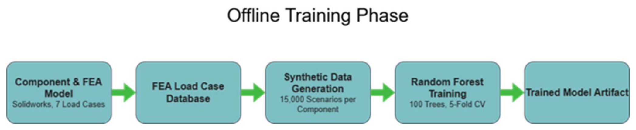
Figure 2.
Detailed data flow diagram of the digital twin pipeline.
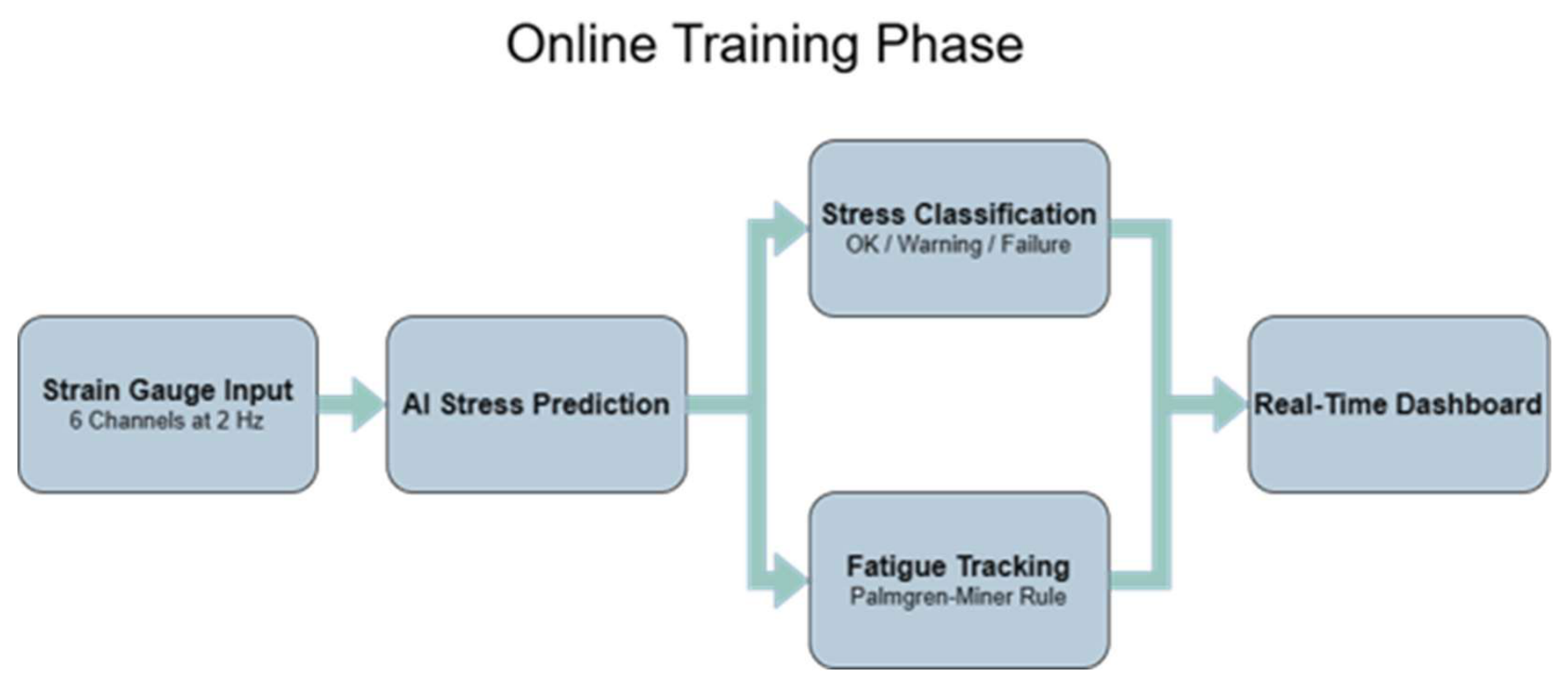
Figure 3.
Flowchart on how the AMIFAIM pipeline works, and what output data we receive.
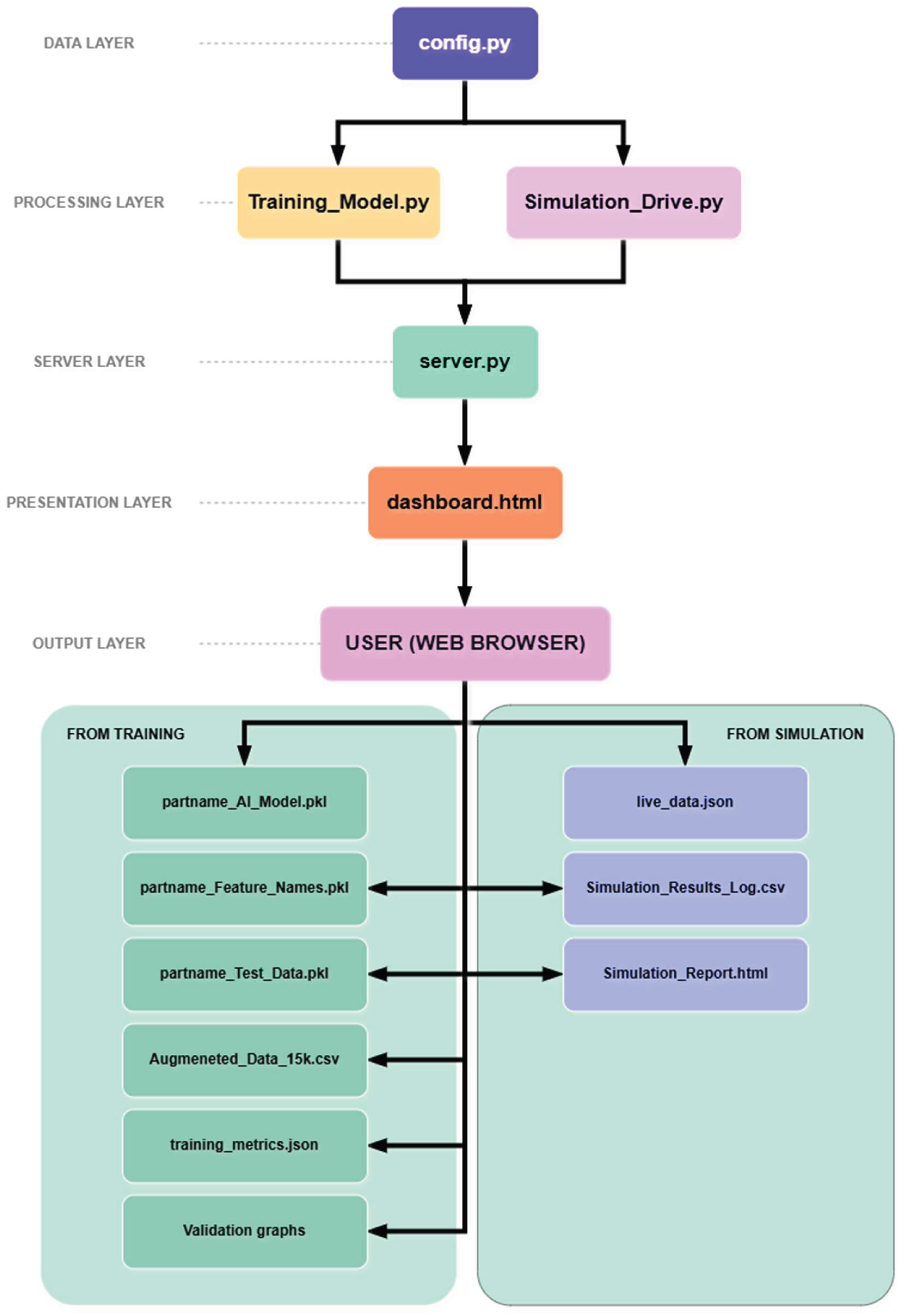
Figure 4.
FEA boundary conditions: (1) distributed load on the ball-joint bore; (2) fixed constraints at both bushing bores.
Figure 4.
FEA boundary conditions: (1) distributed load on the ball-joint bore; (2) fixed constraints at both bushing bores.
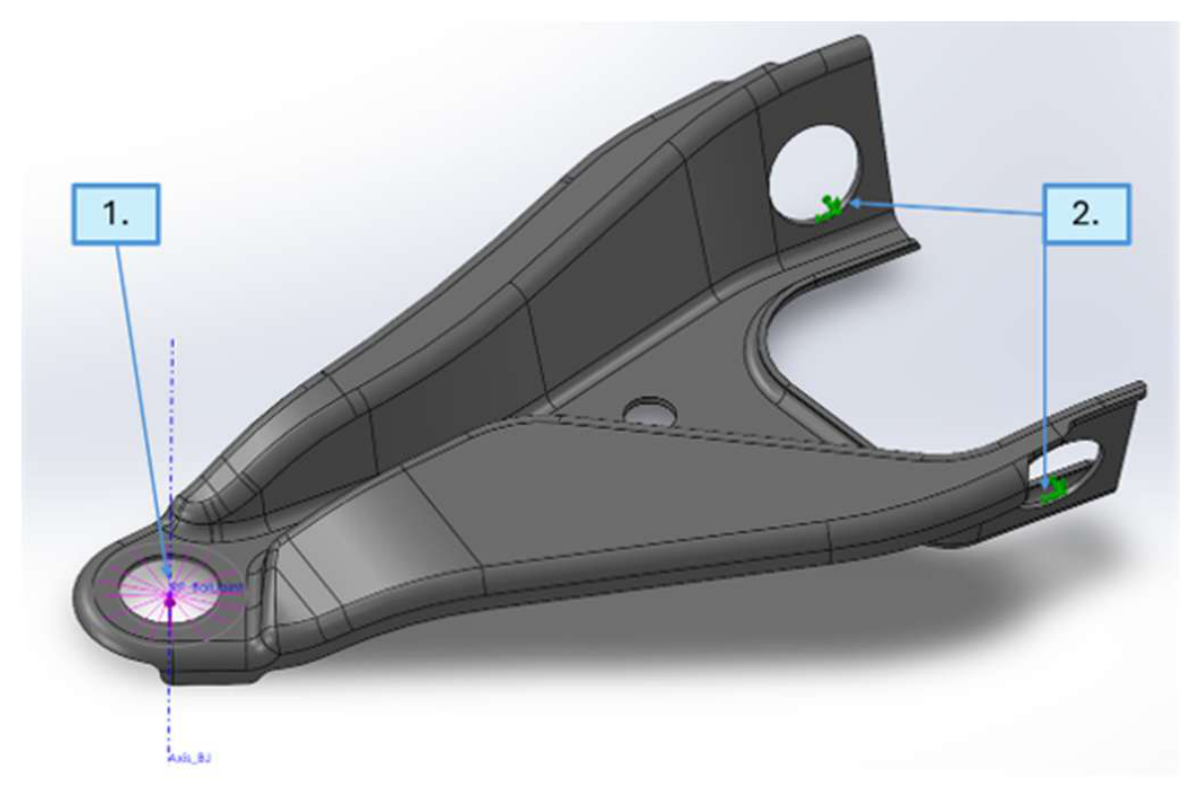
Figure 5.
Sensor signal at 2 Hz (blue curve) with slow thermal drift superimposed (red dotted line – drift amplitude multiplied by a factor of 200 for visual clarity; actual drift ±3 µε over a 33 s thermal cycle).
Figure 5.
Sensor signal at 2 Hz (blue curve) with slow thermal drift superimposed (red dotted line – drift amplitude multiplied by a factor of 200 for visual clarity; actual drift ±3 µε over a 33 s thermal cycle).
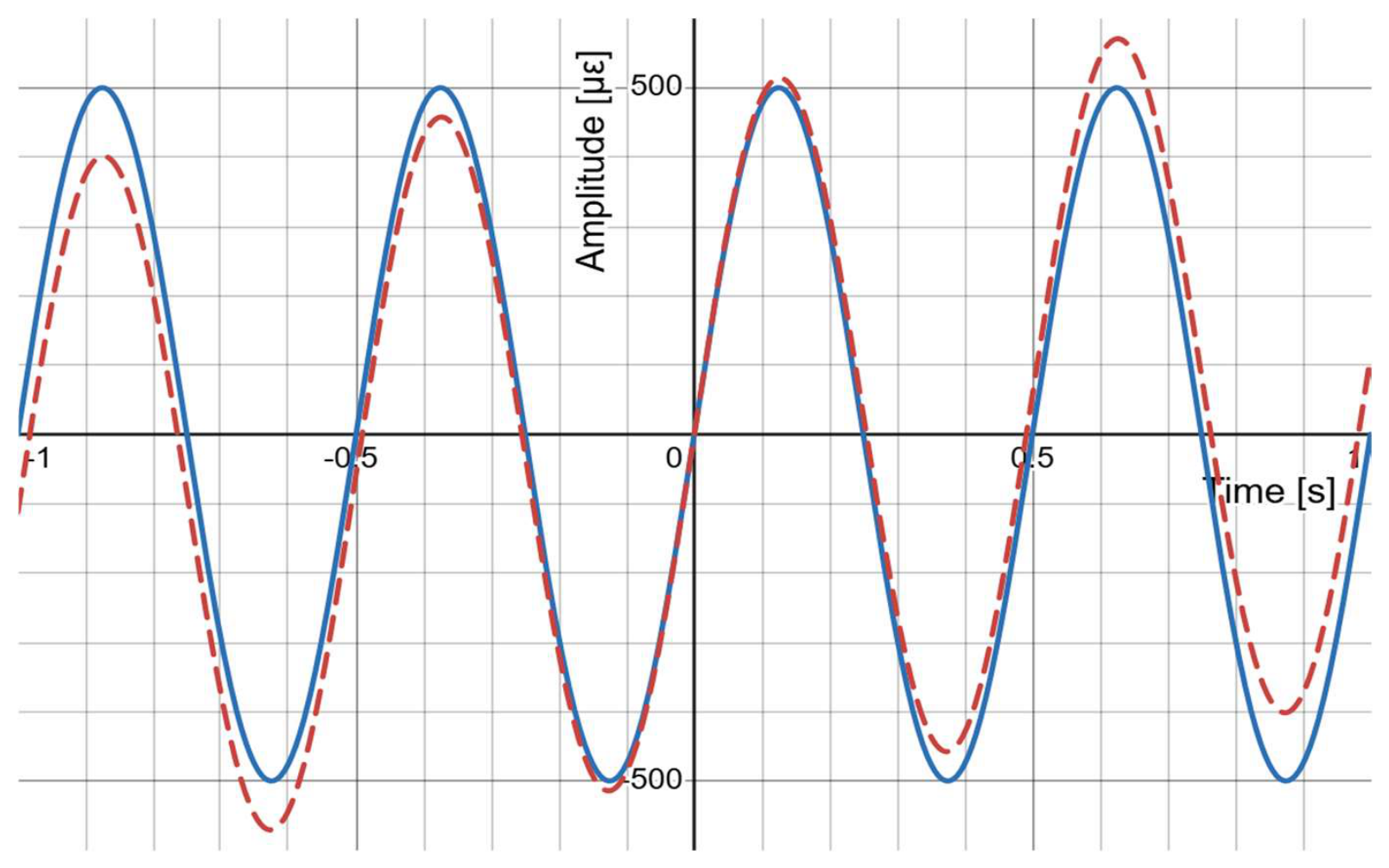
Figure 6.
Scatter plot predicted vs. true Von Mises stress for the 3,000-sample test set, colored by per-prediction uncertainty. Points on the diagonal () are perfect predictions.
Figure 6.
Scatter plot predicted vs. true Von Mises stress for the 3,000-sample test set, colored by per-prediction uncertainty. Points on the diagonal () are perfect predictions.
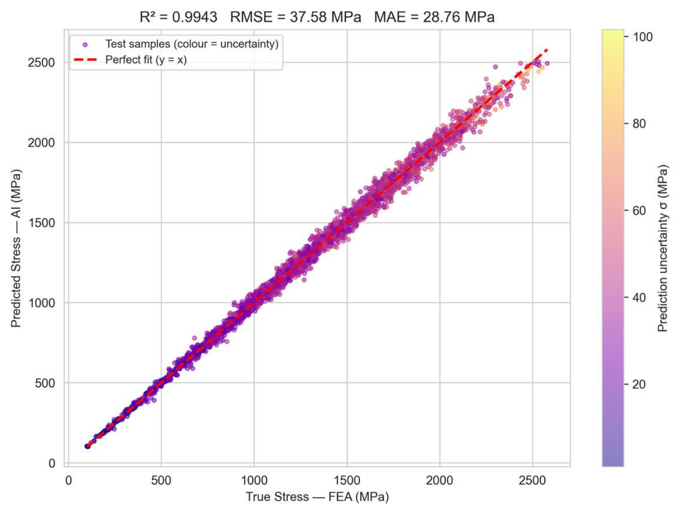
Figure 7.
Residual histogram () for the test set. Orange dashed lines at ±RMSE show the expected error envelope; the symmetric bell curve indicates no systematic bias.
Figure 7.
Residual histogram () for the test set. Orange dashed lines at ±RMSE show the expected error envelope; the symmetric bell curve indicates no systematic bias.
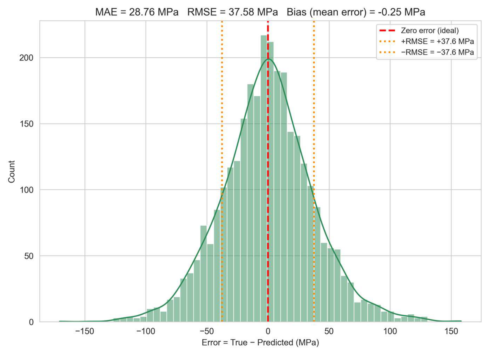
Figure 8.
Random Forest feature importance: each bar shows the fractional contribution of a sensor channel to reducing prediction error across all 100 trees.
Figure 8.
Random Forest feature importance: each bar shows the fractional contribution of a sensor channel to reducing prediction error across all 100 trees.
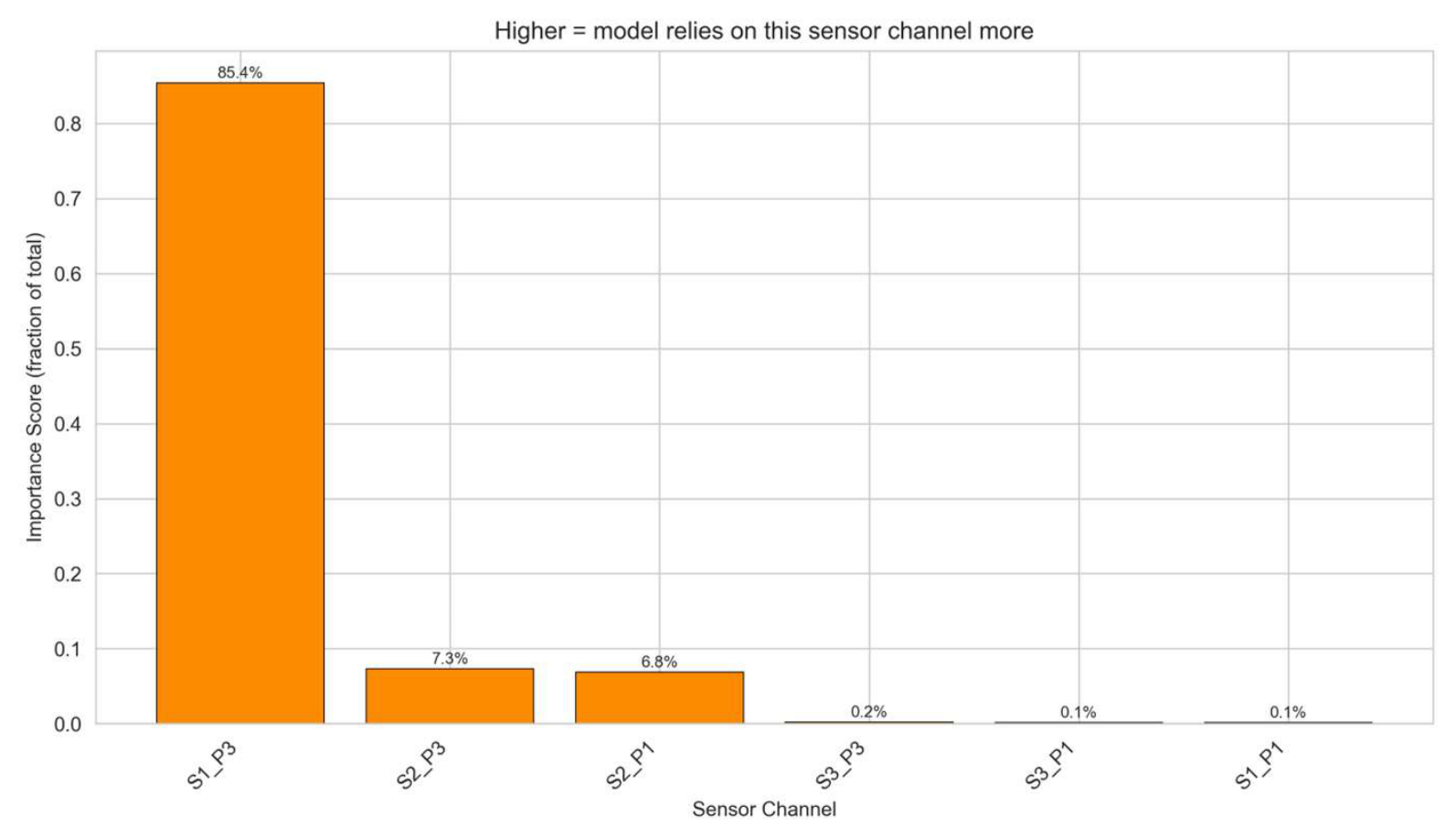
Figure 9.
AI prediction vs. FEA ground truth for 100 sorted test samples. Black curve: FEA stress; red curve: AI prediction; shaded band: ± 1σ uncertainty.
Figure 9.
AI prediction vs. FEA ground truth for 100 sorted test samples. Black curve: FEA stress; red curve: AI prediction; shaded band: ± 1σ uncertainty.
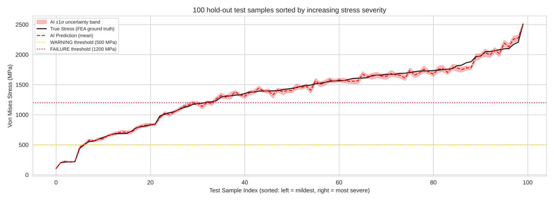
Figure 10.
Visual simulation representation dashboard.
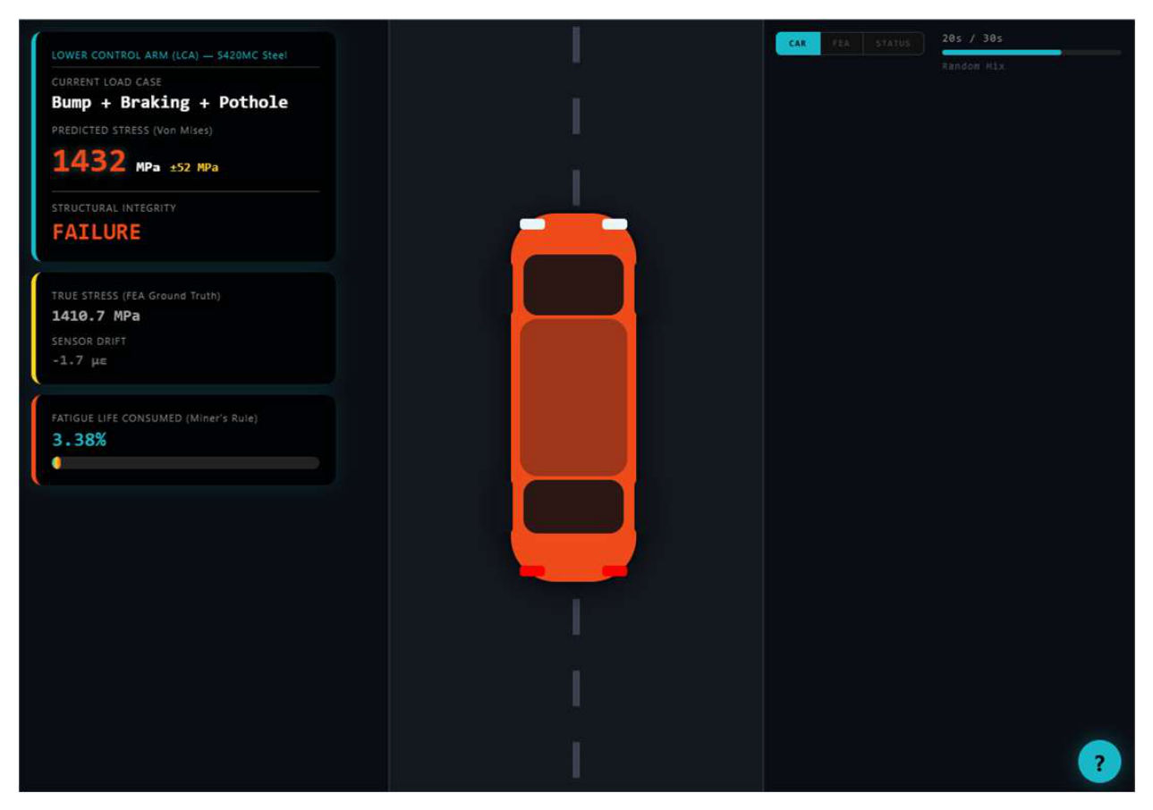
Table 1.
Overview of the seven FEA load cases used in the framework.
| Load Case | Description |
|---|---|
| LC1 | Static + mild bump |
| LC2 | Pothole / curb hit |
| LC3 | Cornering 0.8 g |
| LC4 | Hard braking 1.0 g |
| LC5 | Combined cornering + vertical |
| LC6 | Combined braking + vertical |
| LC7 | Worst practical combination |
Table 2.
Selected properties of S420MC relevant to the LCA model, taken as per EN 10149-2:2013.
| Property | S420MC value / requirement | Relevance for LCA model |
|---|---|---|
| Material designation | S420MC, no. 1.0980 | Hot-rolled micro alloyed steel for cold forming |
| Standard | EN 10149-2 | Reference standard for thermomechanical rolled high-yield-strength steel |
| Min. yield strength, ReH | ≥ 420 MPa | Defines the elastic safety threshold |
| Tensile strength,Rm | 480–620 MPa | Minimum 480 MPa used as UTS in the fatigue model |
| Min. elongation | A₈0 ≥ 16% (t < 3 mm); A ≥ 19% (t ≥ 3 mm) | Confirms sufficient formability for stamped chassis components |
| Carbon content | C ≤ 0.12% | Supports weldability and cold-forming capability |
| Manganese content | Mn ≤ 1.60% | Contributes to strength while maintaining formability |
| Microalloying elements | Nb, V, Ti; Nb + V + Ti ≤ 0.22% | Provides grain refinement and high yield strength |
Table 3.
Complete load matrix for the seven FEA load cases with resulting peak Von Mises stress.
| LC | Description | Fₓ (N) | F_y (N) | F_z (N) | σ_VM,max (MPa) |
|---|---|---|---|---|---|
| 1 | Static + mild bump | 0 | 6,000 | 0 | 1,249 |
| 2 | Pothole / curb hit | 0 | 12,000 | 0 | 2,498 |
| 3 | Cornering 0.8 g | 3,000 | 0 | 0 | 103 |
| 4 | Hard braking 1.0 g | 0 | 0 | -4,500 | 364 |
| 5 | Cornering + bump | 3,000 | 8,000 | 0 | 1,630 |
| 6 | Braking + bump | 0 | 8,000 | -4,000 | 1,812 |
| 7 | Worst combination | 3,000 | 8,000 | -4,000 | 1,776 |
Table 4.
Cycles to failure and time to failure at representative hot-spot stress levels (2 Hz simulation rate).
Table 4.
Cycles to failure and time to failure at representative hot-spot stress levels (2 Hz simulation rate).
| Stress (MPa) | N (cycles to failure) | Time to failure at 2 Hz |
|---|---|---|
| 756 (endurance limit, hot-spot) | ∞ | Never (no damage) |
| 800 | ≈ 38,880 | ≈ 5.4 hours |
| 1,000 | ≈ 12,740 | ≈ 1.8 hours |
| 1,200 | ≈ 5,120 | ≈ 43 minutes |
| 1,500 | ≈ 1,678 | ≈ 14 minutes |
| 2,000 | ≈ 398 | ≈ 3.3 minutes |
| 2,498 (LC2 pothole) | ≈ 131 | ≈ 66 seconds |
Table 5.
Event keyword mapping to stress bands, FEA load cases and stress ranges in the test set.
| Event keyword | Matches test samples with | Corresponding FEA load cases | Typical stress range |
|---|---|---|---|
| Gentle | True stress σ ≤ 500 MPa (OK band) | Mostly cornering and braking blends (LC3, LC4) | 100–500 MPa (163 samples) |
| Moderate | 500 < σ ≤ 1,200 MPa (WARNING band) | Cornering/braking blends with a partial bump or pothole share | 500–1,200 MPa (957 samples) |
| Severe | σ > 1,200 MPa (FAILURE band) | Blends with large LC1, LC2 or LC5–LC7 shares | 1,200–2,580 MPa (1,880 samples) |
Table 7.
Random Forest feature importance ranking for the LCA.
| Rank | Channel | Gauge location | Importance (%) |
|---|---|---|---|
| 1 | S1_P3 | Sensor 1, ε₃ (3rd principal) | 85.4 |
| 2 | S2_P3 | Sensor 2, ε₃ (3rd principal) | 7.3 |
| 3 | S2_P1 | Sensor 2, ε₁ (1st principal) | 6.8 |
| 4 | S3_P3 | Sensor 3, ε₃ (3rd principal) | 0.2 |
| 5 | S3_P1 | Sensor 3, ε₁ (1st principal) | 0.1 |
| 6 | S1_P1 | Sensor 1, ε₁ (1st principal) | 0.1 |
Table 9.
Status distribution across the five drive scenarios (30 s simulations, 2 Hz; mean of four runs per scenario).
Table 9.
Status distribution across the five drive scenarios (30 s simulations, 2 Hz; mean of four runs per scenario).
| Scenario | OK (%) | WARNING (%) | FAILURE (%) | Interpretation |
|---|---|---|---|---|
| Highway cruise | ≈ 94 | ≈ 6 | 0 | Dominated by Gentle events with brief Moderate road-joint spikes. Stress mostly below 500 MPa. |
| City drive | ≈ 66 | ≈ 16 | ≈ 18 | Severe (pothole-type) events produce brief FAILURE spikes. |
| Track day | ≈ 31 | ≈ 36 | ≈ 33 | Alternating Moderate and Severe events keep stress in the WARNING and FAILURE bands. |
| Stress test | ≈ 4 | ≈ 5 | ≈ 92 | Repeated severe impacts; most of the simulation above 1,200 MPa. |
| Random mix | ≈ 5 | ≈ 31 | ≈ 64 | Uniform sampling of the test set, which is dominated by high-stress blends; useful for accuracy verification across the full stress range. |
Table 10.
Fatigue accumulation summary across the five drive scenarios (30 s simulations, 2 Hz, ≈ 57 timesteps; dominant range = 10th–90th percentile of predicted stress; range over four runs per scenario).
Table 10.
Fatigue accumulation summary across the five drive scenarios (30 s simulations, 2 Hz, ≈ 57 timesteps; dominant range = 10th–90th percentile of predicted stress; range over four runs per scenario).
| Scenario | Dominant stress range (MPa) | Fatigue D after 30 s (%) | Projected time to D = 1.0 |
|---|---|---|---|
| Highway cruise | 170–480 | < 0.03 | > 30 hours (almost all below endurance limit) |
| City drive | 180–1,550 with spikes to ≈ 2,300 | ≈ 1–2 | ≈ 25–55 minutes |
| Track day | 290–1,830 | ≈ 2–3 | ≈ 16–26 minutes |
| Stress test | 1,250–2,050 | ≈ 5–8 | ≈ 6–10 minutes |
| Random mix | 700–1,930 | ≈ 4–5 | ≈ 10–12 minutes |
Disclaimer/Publisher’s Note: The statements, opinions and data contained in all publications are solely those of the individual author(s) and contributor(s) and not of MDPI and/or the editor(s). MDPI and/or the editor(s) disclaim responsibility for any injury to people or property resulting from any ideas, methods, instructions or products referred to in the content. |
© 2026 by the authors. Licensee MDPI, Basel, Switzerland. This article is an open access article distributed under the terms and conditions of the Creative Commons Attribution (CC BY) license (http://creativecommons.org/licenses/by/4.0/).
Copyright: This open access article is published under a Creative Commons CC BY 4.0 license, which permit the free download, distribution, and reuse, provided that the author and preprint are cited in any reuse.