

Submitted:
20 October 2026
Posted:
21 October 2026
You are already at the latest version
Abstract
Dissolved organic matter (DOM) regulates carbon cycling, nutrient availability and light attenuation, yet the seasonal coupling between dissolved organic carbon (DOC) quantity and DOM optical quality remains poorly understood in shallow plateau lakes. We tracked monthly environmental conditions, phytoplankton biomass (Chl-a), DOC and DOM optical properties at 11 fixed sites in Lake Erhai, China, over one annual cycle. Principal component analysis explained 73.51% of DOM compositional variance, and PERMANOVA confirmed significant monthly restructuring (R2 = 0.563, p = 0.001), with pronounced transitions in spring (March–April) and late summer (July–September). DOC remained at 4.62–7.01 mg L−1 from November to July and then rose abruptly to 20.51–24.73 mg L−1 during August–October; month alone explained almost all DOC variation (adjusted R2 = 0.989), whereas Chl-a, water temperature, nutrients and location had no independent effects. Chl-a varied non-monotonically, being negatively associated with dissolved inorganic nitrogen and positively with dissolved inorganic phosphorus. Environmental and DOM transition distances were only moderately and non-significantly correlated (r = 0.382, p = 0.28), indicating asynchronous kinetics. The late-season DOC surge was decoupled from contemporaneous algal biomass, revealing a fundamental quantity–quality uncoupling within the lake’s organic carbon pool and underscoring the value of optical characterization in carbon monitoring.
Keywords:
dissolved organic matter
; optical properties
; chlorophyll-a
; Lake Erhai
1. Introduction
Dissolved organic matter (DOM) is a dynamic component of lake ecosystems that influences aquatic carbon cycling, nutrient availability, light attenuation, and microbial metabolism [1]. Its ecological significance depends not only on its concentration but also on its optical composition, which reflects differences in molecular characteristics, source contributions, and biogeochemical processing [2,3]. Ultraviolet–visible absorption and fluorescence indices provide complementary information on DOM characteristics, allowing changes in DOM abundance (via absorption or fluorescence intensity) to be distinguished from changes in its optical properties and compositional quality [4,5,6]. However, these characteristics do not necessarily vary synchronously because DOM concentration and composition can respond differently to biological production, external inputs, and in-lake processing [3,7].
Temporal variability is a prominent feature of DOM in lakes. Seasonal changes in temperature, hydrological conditions, nutrient availability, and primary production can alter both DOM concentration and its optical characteristics [7,8]. Nevertheless, a seasonal classification alone may obscure important differences among individual months. DOM may change gradually during some periods but undergo relatively abrupt shifts during others. These transitions are ecologically relevant because they identify periods when the characteristics of the DOM pool change most strongly. Although previous studies have documented seasonal variation in lake DOM, including research on the optical characteristics of DOM in Lake Erhai, the extent to which monthly changes in DOM concentration and optical composition follow the same temporal trajectory remains insufficiently resolved [5,9]. In particular, identifying whether consecutive months differ consistently in multivariate DOM characteristics can provide a more detailed description of temporal variability than comparisons between broadly defined seasons.
The relationship between DOM and phytoplankton provides a further reason to distinguish DOM concentration from composition [10,11]. Phytoplankton can contribute organic matter through exudation, cell lysis and degradation, while DOM can also originate from other biological processes and external inputs [12,13]. Chlorophyll-a (Chl-a) is commonly used as an proxy of phytoplankton biomass, but its relationship with DOM may vary with nutrient conditions, selective DOM processing, and the temporal scale of observation [14]. Water temperature and nutrient concentrations often exhibit seasonal covariation, complicating the separation of their individual statistical associations from the broader seasonal patterns represented by month [2,15,16]. Analyses that do not account for temporal structure may therefore attribute to individual environmental variables patterns that primarily reflect differences among months. Evaluating DOM–environment relationships while explicitly accounting for month and sampling location is necessary to determine whether observed associations persist beyond these temporal and spatial structures.
Lake Erhai, a large plateau lake in southwestern China, provides a relevant setting for examining these relationships. Previous research has characterized the optical properties of Erhai DOM and investigated its relationship with phytoplankton, establishing the importance of biological processes in understanding DOM variability [10]. However, a more detailed assessment of monthly observations can address a complementary question: whether changes in DOM abundance, optical composition, and associated environmental conditions are temporally synchronized or instead follow distinct trajectories. This distinction is important for interpreting DOM dynamics because an increase in dissolved organic carbon (DOC) does not necessarily coincide with corresponding changes in DOM optical properties, and temporal coincidence alone does not establish a direct causal relationship with biological or environmental drivers [2,17,18].
In this study, we analyzed monthly observations of water chemistry, Chl-a, DOC, and DOM optical indices from 11 fixed sampling locations in Lake Erhai over a one-year cycle. This study combines multivariate statistical analysis with regression and correlation approaches to characterize temporal variation in DOM and assess its associations with environmental conditions. We propose the following hypotheses: (1) how do the multivariate characteristics of DOM vary among months, and during which month-to-month transitions are the changes most pronounced? (2) does DOC follow the same temporal trajectory as the optical characteristics of DOM, and how much of its variation is associated with month after accounting for Chl-a, water temperature, nutrients, and sampling location? and (3) do Chl-a and environmental variables exhibit independent associations with DOM-related responses after temporal and spatial structure is considered? We expected that monthly variation would be evident in both DOM concentration and optical composition, but that these dimensions would not necessarily change synchronously. By separating temporal patterns from conditional associations with environmental variables, this study provides a more detailed assessment of monthly DOM variability in a plateau lake.
2. Materials and Methods
2.1. Study Site and Sampling Design
Water samples were collected monthly at 11 fixed locations in Lake Erhai from November 2023 to October 2024, covering 12 consecutive sampling months. The sampling design yielded 132 potential site–month observations (11 locations × 12 months; Figure 1). At each sampling location, water temperature, pH, nutrient concentrations, Chl-a, DOC, and optical indices related to dissolved organic matter (DOM) were measured or determined. Surface water (0.5 m depth) was gathered using clean polyethylene bags and promptly transported to the laboratory for analysis. The samples were categorized into two groups: one portion was filtered through a Whatman GF/C filter for water quality parameter analysis, while the other was prepared for CDOM and FDOM spectral analyses. This involved filtering through a precombusted (450 °C, 3 hours) Whatman GF/F filter and a 0.2 μm Millipore filter, followed by storage in 150 mL acid-washed amber glass bottles.
2.2. Physicochemical and Nutrient Measurements
Water temperature and pH were measured using YSI. Total nitrogen (TN), total phosphorus (TP), ammonium nitrogen (NH4+-N), nitrate nitrogen (NO3−-N), and phosphate phosphorus (PO43−-P) refer to the Environmental Quality Standards for Surface Water (GB 3838-2002, China). The Chl-a was obtained by extraction with 90% alcohol.
2.3. Dissolved Organic Carbon and Optical Measurements
The DOC was analyzed by high-temperature catalytic oxidation using a TOC-L Analyzer (Shimadzu, Japan). Absorption spectra of CDOM were measured using a UV-2550 UV–Vis spectrophotometer (Shimadzu, Japan). Spectral slopes S275–295 and S350–400 were calculated using least squares fitting [19]. S275-295 provides insights into DOM composition, molecular weight, and photochemical reactivity [20,21]. The S275–295/S350–400 ratio (SR) serves as a proxy for DOM’s molecular weight, indicative of its source and composition [20]. SUVA254, the ratio of absorbance at 254 nm to DOC concentration [22], and the parameter M, the ratio of absorption coefficients at 250 nm and 365 nm reflecting molecular weight [20], were also calculated.
Fluorescence EEM spectroscopy was performed using a Cary Eclipse spectrometer (Agilent, Malaysia). Both excitation (Ex) and emission (Em) slits were set to 5 nm, with the excitation wavelength ranging from 210–450 nm (5 nm intervals) and emission from 250 to 600 nm (1 nm intervals). Component numbers were determined through split-half and load analyses. The Biogenic Index (BIX) is the ratio of emission (380–430 nm) to excitation (310 nm) wavelengths [23,24], while the Fluorescence Index (FI) is the emission (470–520 nm) to excitation (370 nm) ratio [25]. Fn(355), indicating the relative concentration of humic-like compounds, is the intensity of the emission spectrum at λEM = 450 nm with λEX = 355 nm excitation [26].
2.4. Statistical Analysis
All statistical analyses were performed in RStudio (V4.5.2). Data processing and visualization were conducted using the tidyverse and ggplot2 packages. Statistical significance was evaluated at (p < 0.05). All statistical analyses were conducted in R. Descriptive statistics, including the mean, standard deviation (SD), and median, were calculated for the measured environmental variables and DOM optical indices for each sampling month. The coefficient of variation (CV) was used to characterize within-month spatial variability in selected variables and was calculated as the ratio of the SD to the mean, expressed as a percentage. Monthly summaries were used to examine temporal variation in water temperature, nutrients, Chl-a, DOC, and DOM optical properties across the sampling period.
Principal component analysis (PCA) was used to summarize multivariate variation in environmental conditions and DOM characteristics. Environmental PCA was performed using standardized environmental variables, including water temperature, TN, TP, ammonium nitrogen NH4+–N, NO3−–N, PO43−–P, and Chl-a. DOM PCA was performed separately using standardized DOC concentrations and optical indices, including BIX, FI, Fn355, S275–295, SR, SUVA254, the M, and a(440). PCA was based on centered and scaled variables, and the first principal component axes were used to summarize the dominant multivariate gradients. Monthly mean PCA scores were calculated to characterize temporal changes in environmental and DOM states.
Differences in multivariate composition among months were evaluated using permutational multivariate analysis of variance (PERMANOVA), implemented with the adonis2 function in the vegan package. Environmental variables and DOM properties were analyzed separately. Variables were standardized before Euclidean distance matrices were calculated, and month was included as the explanatory factor. Statistical significance was assessed using 999 permutations. Multivariate dispersion among months was assessed using the betadisper function, followed by analysis of variance, to determine whether differences in within-month dispersion could contribute to the observed PERMANOVA results. Pairwise PERMANOVA comparisons among months were conducted where appropriate, and the resulting p-values were adjusted using the Benjamini–Hochberg procedure to control the false discovery rate.
To examine the relationships between environmental conditions and Chl-a, dissolved inorganic nitrogen (DIN) was calculated as NH4+–N plus NO3−–N, and dissolved inorganic phosphorus (DIP) was represented by PO43−–P. Chl-a was log-transformed as log(1+Chl-a) to reduce skewness. A series of nested linear models was fitted to evaluate the additional explanatory contributions of month, water temperature, DIN, and DIP while accounting for sampling location. The models included location alone, month and location, month and water temperature and location, and month, water temperature, DIN, DIP, and location. Nested models were compared using likelihood-ratio tests, with the test statistic, degrees of freedom, and p-value reported where applicable. Variance inflation factors (VIF) were examined to assess potential multicollinearity among explanatory variables. DOC variation was analyzed using linear models with log(1+DOC) as the response variable. Month, log(1+Chl-a), water temperature, TN, TP, and sampling location were included as explanatory terms to evaluate whether DOC variation was associated with temporal variation, Chl-a, and measured environmental conditions.
To examine temporal correspondence between environmental and DOM variation, monthly mean scores on the first two environmental and DOM principal component axes were used to calculate Euclidean distances between consecutive months within each PCA space. These distances represented the magnitude of month-to-month change in the corresponding multivariate state. Spearman rank correlation was used to test the association between environmental and DOM transition distances. Associations between individual environmental and DOM PCA axes were also examined using Spearman rank correlations. These analyses were considered exploratory because they were based on only 12 monthly observations. All statistical tests were two-sided, and p < 0.05 was used as the nominal significance threshold.
3. Results
3.1. Seasonal Reorganization of Lake Physicochemical and Nutrient Conditions
The measured environmental variables exhibited pronounced seasonal variability across the annual sampling period (Figure 2). Water temperature increased from 11.49 °C in January to 24.52 °C in August, representing an approximately 2.1-fold difference between the annual minimum and maximum. In contrast, nutrient concentrations did not follow the same seasonal trajectory. TN was highest in April (0.81 mg/L) and lowest in August (0.42 mg/L), whereas TP showed a substantially larger seasonal range, increasing to 0.062 mg/L in June but declining to 0.006 mg/L in September. Thus, the seasonal variation in nutrient concentrations was not synchronized with the annual variation in water temperature. Chl-a also exhibited a non-monotonic seasonal pattern. Its mean concentration ranged from 12.41 μg/L in June to 22.02 μg/L in May, with relatively high values occurring again in September (21.21 μg/L) and October (20.53 μg/L). In contrast, DOC showed a distinct late-season increase. Mean DOC remained between 4.62 mg/L and 7.01 mg/L during November–July, but increased sharply to 20.51 mg/L, 23.90 mg/L, and 24.73 mg/L in August, September, and October, respectively. The maximum DOC concentration was therefore approximately 5.4 times the November value.
Collectively, these asynchronous changes drove a substantial seasonal reorganization of the lake’s overall environmental state (PERMANOVA, R2 = 0.537, p < 0.001). Rather than following a simple monotonic trajectory, the lake transitioned dynamically through complex, multidimensional environmental states over the year (Figure 3).
3.2. Seasonal Decoupling Between Phytoplankton Biomass and Hydrological–Nutrient Conditions
Phytoplankton dynamics (indexed by Chl-a) exhibited a non-monotonic seasonal trajectory that was fundamentally decoupled from water temperature (Figure 4). Although Chl-a peaked during May (22.02 μg/L) and early autumn (September–October: >20 μg/L), it dropped to its annual minimum in June (12.41 μg/L)—coinciding with elevated water temperature and the annual peak in TP. Once explicitly accounting for seasonal (Month) and spatial (Location) structures, water temperature exerted no significant effect on Chl-a (β = -0.029, p = 0.570). Instead, inorganic nutrients emerged as the primary drivers: DIN was negatively associated with log-transformed Chl-a, whereas DIP was positively associated with it (β = -2.297 and 12.408, respectively; p = 0.002). The strong intrinsic month effect (p < 0.01) further reflected this seasonal nutrient restructuring. Furthermore, Chl-a dynamics correlated weakly with TN/TP (r = 0.184, p = 0.035) and showed no association with DIN/DIP (r = 0.133, p = 0.149), demonstrating that phytoplankton biomass was governed by broader seasonal nutrient reorganization rather than simple stoichiometry or thermal control alone.
3.3. Pronounced Late-Season Accumulation of DOC
DOC displayed a distinct seasonal trajectory that fundamentally decoupled from phytoplankton biomass. Following a stable baseline during November–July (4.62–7.01 mg/L), DOC accumulated abruptly during August–October, reaching an annual maximum of 24.73 mg/L (Figure 5). Notably, this late-season surge occurred without a corresponding increase in algal biomass (Chl-a: 14.48–21.21 μg/L). Multiple linear regression confirmed that this DOC accumulation represented a strong, intrinsic seasonal signal rather than an artifact of algal production, thermal forcing, or spatial heterogeneity. Seasonal timing (Month) accounted for virtually all variation in log-transformed DOC (R2adj = 0.989, p < 0.001), whereas Chl-a, water temperature, TN, TP, and Location exerted no significant independent effects (p > 0.13 for all). Dropping Month from the full model resulted in a dramatic collapse in explanatory power (residual sum of squares rising from 0.376 to 27.083), whereas removing any other covariate caused negligible changes in model fit. A simplified regime analysis further confirmed that the late-season period (August–October) represented a distinct, highly stable biogeochemical state (β = 1.286, p < 0.001; R2 = 0.951), demonstrating that late-season DOC accumulation is a robust system-level phenomenon rather than a transient monthly anomaly.
3.4. Seasonal Reorganization of DOM Compositional Quality
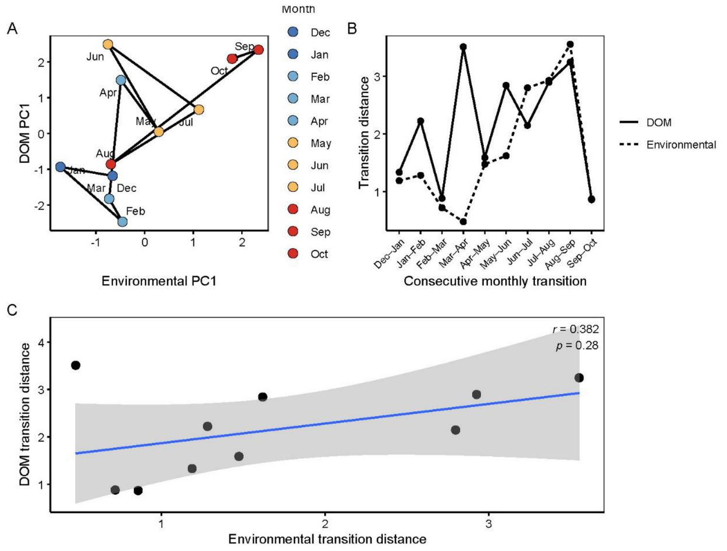
The physical accumulation of DOC was accompanied by substantial shifts in DOM optical properties, reflecting a dynamic evolution of DOM structural quality across the annual cycle. Indicators of molecular weight and aromaticity (SUVA254 and a440) rose during early summer (June: 1.23 L mg−1 m−1 and 0.661 m−1, respectively), while markers of autochthonous biological activity (BIX and FI) increased progressively toward late autumn (peaking at 0.983 and 2.15 in October). PCA resolved these optical traits into three major compositional axes (73.51% cumulative variance explained). DOM-PC1 (43.2% variance) represented chromophoric, high-molecular-weight DOM, driven by positive loadings of a440, SR, and SUVA254 against negative loadings of S275₋295 and M. DOM-PC2 (18%) indexed DOM quantity and humic fluorescence (DOC, Fn355), while DOM-PC3 (12.4%) captured biological/autochthonous contributions (BIX, FI) (Figure 6). The seasonal trajectories of these PC scores revealed distinct compositional transitions: DOM-PC1 shifted from negative values in winter to strongly positive values from April through October (peaking in June at 2.50), reflecting a shift toward more aromatic DOM. In contrast, DOM-PC2 spiked sharply during August–October (up to 2.02), tracking late-season organic accumulation. Critically, the magnitude of month-to-month DOM compositional shifts did not strictly mirror bulk environmental changes. DOM transition distances peaked sharply during spring (March–April: 3.51) and late summer/autumn (July–September: 2.84–3.24), whereas bulk environmental transition distances peaked in late summer (August–September: 3.70) (Figure 7B). The correlation between DOM and environmental transition rates was moderate and statistically non-significant (r = 0.382, p = 0.28; Figure 7C), indicating that while bulk environmental drivers and DOM composition are coupled on an annual scale, DOM quality reorganizes with distinct, asynchronous kinetic trajectories between sampling intervals.
4. Discussion
4.1. Seasonal Environmental Variability and Phytoplankton Responses
The seasonal pattern observed in Lake Erhai was not adequately represented by a single temperature-related gradient [27,28]. Although water temperature increased from its winter minimum to a summer maximum, total nitrogen, total phosphorus, and chlorophyll-a followed distinct trajectories. TP reached its annual maximum in June, when Chl-a was at its minimum, whereas Chl-a peaked in May and remained relatively high again in September and October. This mismatch indicates that seasonal thermal conditions, nutrient concentrations, and phytoplankton standing stock did not vary proportionally.
Such differences are consistent with studies showing that chlorophyll–nutrient relationships vary with season, lake characteristics, and additional ecological controls [28,29]. In a long-term analysis of Lake Taihu, the relationship between Chl-a and nutrients changed over time, and water-column stability and light conditions contributed to the observed variation in algal responses to nutrients. Across subtropical shallow lakes, the relative importance of TP and water temperature also differed between lake types and seasons, demonstrating that nutrient concentrations alone do not consistently predict Chl-a [28]. More generally, phytoplankton growth can reflect co-limitation by light and nutrients rather than a response to a single chemical variable [30,31,32].
Beyond the shifts in overall water quality, the seasonal environmental evolution was marked by dynamic changes in internal spatial heterogeneity. Rather than reflecting a uniform lake-wide response, the system transitioned through phases of varying spatial dispersion among sampling sites. Periods with elevated spatial variability likely reflect localized biogeochemical processing—such as spatial differences in macrophyte density, riverine inputs, or shallow sediment resuspension—whereas periods of spatial convergence coincide with enhanced physical mixing. This seasonal expanding and contracting of spatial patchiness underscores that seasonal environmental reorganization in Lake Erhai operates simultaneously across both temporal and spatial scales.
This spatial heterogeneity has profound ecological implications for understanding ecosystem-level biogeochemical buffering. Across lakes, the relationship between DOC and phytoplankton biomass can vary with seasonal light availability and nutrient stoichiometry, rather than following a uniform response [31]. In addition, a monthly sample represents a snapshot of standing concentrations rather than the rates of nutrient loading, biological uptake, regeneration, or loss [33]. These processes can operate simultaneously and can produce different trajectories in total and dissolved nutrient pools. The seasonal environmental trajectory in Lake Erhai reflects a dynamic, multidimensional state transition driven by asynchronous hydro-chemical inputs and biological processing.
4.2. Interpreting the Contrasting Associations of Chl-a with DIN and DIP
The negative association between Chl-a and DIN, alongside the positive association with DIP, does not support a simple classification of Lake Erhai as nitrogen-limited or phosphorus-limited throughout the year [29,34]. Different balances between nutritional supply and biological demand may be reflected in the two relationships. The depletion of dissolved inorganic nitrogen during times of increased phytoplankton consumption is one explanation for the negative DIN relationship [29,35]. In this case, low DIN and high Chl-a would be simultaneous results of biological activity rather than proof that low DIN encouraged phytoplankton development. Alternatively, DIN may have varied with seasonal changes in inputs, recycling, or nitrogen removal that were not captured by the measured variables. The present observations cannot distinguish these possibilities because nutrient uptake and turnover rates were not measured.
The positive DIP relationship would suggest that higher phytoplankton standing stock was also promoted during times of increased phosphorus availability. Nevertheless, phosphorus intake and supply both affect the concentration that remains in the water column. Therefore, a positive statistical correlation does not prove that phosphorus was the only limiting nutrient or that raising phosphorus would inevitably result in a corresponding rise in Chl-a.
The decoupling of stoichiometric ratios (TN/TP and DIN/DIP) from algal biomass emphasizes the dominant role of active biological absorption and rapid internal turnover, despite the fact that these ratios are frequently employed to infer nutrient limitation. The observed depletion of DIN relative to DIP during peak biomass points toward transient nitrogen draw-down rather than absolute N-limitation per se. Chl-a did not significantly correlate with DIN/DIP, although it did exhibit a weak positive correlation with TN/TP. Different nutrient pools are represented by these ratios: DIN/DIP is limited to dissolved inorganic forms, while TN/TP covers total nutrient components. Their interactions with Chl-a do not have to be the same, especially when absorption and recycling alter nutrient availability. Nutrient ratios can indicate potential imbalance, but they do not directly measure phytoplankton responses to nutrient addition [36]. Research on subtropical shallow lakes has likewise documented variation in nutrient–Chl-a relationships across seasons and lake types [28], while broader lake studies show that nutrient relationships depend on trophic status and other environmental conditions.
4.3. Late-Season DOC Accumulation and Its Relationship to DOM Properties
DOC remained within a relatively narrow range from November through July before increasing sharply in August and remaining high through October. Chl-a did not rise concurrently; throughout July and August, DOC increased while Chl-a decreased. After taking month and location into consideration, the DOC model did not find any independent correlations with Chl-a, water temperature, TN, or TP. Although the late-season increase in DOC is statistically significant, a mix of hydroclimatic triggers and delayed biological legacies is probably the mechanism behind it. For example, this late-season carbon pulse could be driven by the breakdown of macrophyte residues or post-bloom phytoplankton detritus [37], along with increased sediment organic carbon release under warm conditions, without needing a contemporaneous increase in active Chl-a biomass.
Phytoplankton can contribute DOM through exudation, cell turnover, and decomposition, but the amount of DOC present at a given time reflects the balance between production and removal [33,38]. Organic matter released earlier may remain in the water after Chl-a declines, while microbial processing and photochemical reactions may alter its persistence and properties [15,39]. DOC may also be affected by external inputs and water exchange [40,41,42]. Seasonal studies of large Chinese lakes have documented changes in DOM quantity, composition, and lability over the annual cycle [7,43]. Hydrological studies have further shown that changes in water exchange can alter DOM chemistry in lake systems, including Poyang Lake [41,42]. These findings identify plausible processes for comparison, but they do not establish the cause of the DOC increase in Lake Erhai.
Although maximum DOC levels coincided with the warmer summer period, temperature per se did not directly drive this organic carbon accumulation. Thermal regimes in Lake Erhai are intrinsically linked to broader seasonal environmental restructuring. Once seasonal timing is controlled, temperature provides no additional predictive power, demonstrating that the late-season carbon buildup reflects an integrated ecosystem response rather than direct thermal forcing. Likewise, the consistency of this surge across all sampling sites highlights that late-season DOC accumulation is a robust, lake-wide phenomenon governed by broad-scale seasonal drivers rather than spatially heterogeneous inputs.
DOC concentration and DOM optical properties provide different information about this accumulation. DOC quantifies the amount of dissolved organic carbon, whereas absorption and fluorescence indices characterize selected properties of the dissolved pool. A rise in DOC need not be accompanied by a proportional change in aromaticity-related indicators, spectral slopes, or fluorescence [44]. Conversely, optical properties may change as DOM is processed even when DOC concentration changes little. Studies of DOM in lakes have shown that trophic state, phytoplankton succession, and hydrological conditions can be associated with changes in DOM composition [3].
The late-season DOC increase is therefore a clear concentration pattern, but its source and fate remain unresolved. Distinguishing increased external inputs from enhanced in-lake production or reduced removal would require additional evidence, such as inflow and outflow measurements, DOM molecular characterization, and measurements of biological processing [15]. The current data establish when DOC accumulated and how its optical properties varied alongside that accumulation; they do not identify a single pathway responsible for it.
These results do not exclude a contribution of phytoplankton to DOM production. Rather, they indicate that the observed DOC concentration pattern cannot be explained by contemporaneous Chl-a alone. Phytoplankton-derived organic matter can enter the dissolved pool through exudation, cell turnover, and decomposition, but DOC concentration is also affected by microbial processing, photochemical alteration, dilution, transport, and other inputs. These processes need not peak at the same time as standing Chl-a. For example, studies of lake systems have documented seasonal differences in DOM quantity and composition that reflect changing balances between hydrological inputs and internal biological production. Research on DOC gradients across thousands of lakes has also shown that the relationship between DOC and Chl-a depends on seasonal light and nutrient conditions rather than following a uniform response.
4.4. Implications for Interpreting Seasonal Water Quality
These findings illustrate why chlorophyll-a, nutrient pools, DOC concentrations, and optical indices offer complementary rather than interchangeable perspectives on lake ecosystems. Because these variables respond to distinct biogeochemical mechanisms and operate on varying timescales, their seasonal trajectories frequently diverge. For instance, evaluating lake condition based solely on phytoplankton standing stock or bulk nutrient levels can sometimes overlook important internal shifts, such as the pronounced late-season organic carbon accumulation observed in this system.
This divergence carries useful implications for environmental monitoring and ecological assessment. While routine parameters remain essential for tracking primary productivity and nutrient loading, incorporating DOM optical characterization provides a more comprehensive view of organic matter dynamics. Such multi-parameter approaches can help prevent potential misinterpretations of ecosystem status during periods when biological biomass and carbon cycling are uncoupled. Nonetheless, given that these insights derive from a single annual cycle in one plateau system, broader applications would benefit from multi-year observations and comparative studies across diverse lake types to better understand how widely these asynchronous patterns occur.
5. Conclusions
Monthly monitoring in Lake Erhai demonstrates that seasonal environmental forcing, phytoplankton standing stock, dissolved organic carbon accumulation, and dissolved organic matter optical traits evolve along asynchronous kinetic trajectories. Phytoplankton biomass was governed by seasonal nutrient restructuring—specifically inorganic nitrogen drawdown and phosphorus availability—rather than direct thermal control. The defining feature of the lake’s carbon dynamics was a pronounced late-season organic carbon pulse during late summer and autumn, which was decoupled from contemporaneous algal biomass, water temperature, nutrient levels, and spatial heterogeneity. Concurrently, shifts in optical indicators reflected distinct qualitative transformations, highlighting a fundamental quantity–quality uncoupling within the dissolved organic carbon reservoir.
These findings demonstrate that bulk nutrient concentrations, chlorophyll-a biomass, and organic carbon pools represent functionally distinct dimensions of water quality that cannot be treated as interchangeable proxies. Effective ecosystem assessment in shallow plateau lakes requires an integrated framework that combines routine concentration metrics with spectroscopic characterization to capture asynchronous biogeochemical shifts. Disentangling the exact mechanisms driving this late-season carbon pulse will ultimately require multi-year observations incorporating hydrological flux accounting, sediment diffusion measurements, and molecular-level organic characterization.
Author Contributions
Conceptualization, D.H. and Y.G.; methodology, Y.G.; software, Y.G.; validation, Y.G.; formal analysis, Y.G.; investigation, Y.G.; data curation, Y.G.; writing—original draft preparation, Y.G.; writing—review and editing, D.H.; visualization, Y.G.; supervision, D.H.; project administration, D.H.; funding acquisition, D.H. All authors have read and agreed to the published version of the manuscript.
Funding
This research was funded by the Science and Technology Program of Inner Mongolia Autonomous Region, grant number 2025YFDZ0054; the China Postdoctoral Science Foundation, grant number 2021M703430; and the National Natural Science Foundation of China, grant number 32361133561.
Data Availability Statement
The data presented in this study are available on request from the corresponding author.
Conflicts of Interest
The authors declare no conflicts of interest.
References
- Johnes, P.J.; Evershed, R.P.; Jones, D.L.; Maberly, S.C. Exploring the Nature, Origins and Ecological Significance of Dissolved Organic Matter in Freshwaters: State of the Science and New Directions. Biogeochemistry 2023, 164, 1–12. [Google Scholar] [CrossRef]
- D’Andrilli, J.; Silverman, V.; Buckley, S.; Rosario-Ortiz, F.L. Inferring Ecosystem Function from Dissolved Organic Matter Optical Properties: A Critical Review. Environ. Sci. Technol. 2022, 56, 11146–11161. [Google Scholar] [CrossRef] [PubMed]
- Wen, Z.; Shang, Y.; Song, K.; Liu, G.; Hou, J.; Lyu, L.; Tao, H.; Li, S.; He, C.; Shi, Q.; He, D. Composition of Dissolved Organic Matter (DOM) in Lakes Responds to the Trophic State and Phytoplankton Community Succession. Water Res. 2022, 224, 119073. [Google Scholar] [CrossRef] [PubMed]
- Fellman, J.B.; Hood, E.; Spencer, R.G.M. Fluorescence Spectroscopy Opens New Windows into Dissolved Organic Matter Dynamics in Freshwater Ecosystems: A Review. Limnol. Oceanogr. 2010, 55, 2452–2462. [Google Scholar] [CrossRef]
- Guan, Y.; Yu, G.; Jia, N.; Han, R.; Huo, D. Spectral Characteristics of Dissolved Organic Matter in Plateau Lakes: Identifying Eutrophication Indicators in Southwest China. Ecol. Inform. 2024, 82, 102703. [Google Scholar] [CrossRef]
- Stedmon, C.A.; Markager, S. Tracing the Production and Degradation of Autochthonous Fractions of Dissolved Organic Matter by Fluorescence Analysis. Limnol. Oceanogr. 2005, 50, 1415–1426. [Google Scholar] [CrossRef]
- Huang, Q.; Liu, L.; Huang, J.; Chi, D.; Devlin, A.T.; Wu, H. Seasonal Dynamics of Chromophoric Dissolved Organic Matter in Poyang Lake, the Largest Freshwater Lake in China. J. Hydrol. 2022, 605, 127298. [Google Scholar] [CrossRef]
- Kurek, M.R.; Frey, K.E.; Guillemette, F.; Podgorski, D.C.; Townsend-Small, A.; Arp, C.D.; Kellerman, A.M.; Spencer, R.G.M. Trapped Under Ice: Spatial and Seasonal Dynamics of Dissolved Organic Matter Composition in Tundra Lakes. J. Geophys. Res. Biogeosci. 2022, 127, e2021JG006578. [Google Scholar] [CrossRef]
- Li, Z.; Fu, Z.; Zhang, Y.; Guo, Y.; Che, F.; Guo, H.; Wang, S. Temporal and Spatial Distribution and Fluorescence Spectra of Dissolved Organic Matter in Plateau Lakes: A Case Study of Qinghai Lake. Water 2021, 13, 3481. [Google Scholar] [CrossRef]
- Guan, Y.; Han, R.; Jia, N.; Yu, G.; Huo, D. Optical Characteristics of Dissolved Organic Matter in Relation to Phytoplankton in Lake Erhai, China. Process Saf. Environ. Prot. 2024, 186, 166–175. [Google Scholar] [CrossRef]
- Zhang, Y.; Yang, F.; Liao, H.; Hu, S.; Yu, H.; Yuan, P.; Li, B.; Cui, B. Variation in Spectral Characteristics of Dissolved Organic Matter and Its Relationship with Phytoplankton of Eutrophic Shallow Lakes in Spring and Summer. Water 2022, 14, 2999. [Google Scholar] [CrossRef]
- Baines, S.B.; Pace, M.L. The Production of Dissolved Organic Matter by Phytoplankton and Its Importance to Bacteria: Patterns across Marine and Freshwater Systems. Limnol. Oceanogr. 1991, 36, 1078–1090. [Google Scholar] [CrossRef]
- Thornton, D.C.O. Dissolved Organic Matter (DOM) Release by Phytoplankton in the Contemporary and Future Ocean. Eur. J. Phycol. 2014, 49, 20–46. [Google Scholar] [CrossRef]
- Bracchini, L.; Dattilo, A.M.; Hull, V.; Loiselle, S.A.; Nannicini, L.; Picchi, M.P.; Ricci, M.; Santinelli, C.; Seritti, A.; Tognazzi, A.; Rossi, C. Spatial and Seasonal Changes in Optical Properties of Autochthonous and Allochthonous Chromophoric Dissolved Organic Matter in a Stratified Mountain Lake. Photochem. Photobiol. Sci. 2010, 9, 304–314. [Google Scholar] [CrossRef] [PubMed]
- Andersson, A.; Powers, L.; Harir, M.; Gonsior, M.; Hertkorn, N.; Schmitt-Kopplin, P.; Kylin, H.; Hellström, D.; Pettersson, Ä.; Bastviken, D. Molecular Level Seasonality of Dissolved Organic Matter in Freshwater and Its Impact on Drinking Water Treatment. Environ. Sci. Water Res. Technol. 2024, 10, 1964–1981. [Google Scholar] [CrossRef]
- Thottathil, S.D.; Hayakawa, K.; Hodoki, Y.; Yoshimizu, C.; Kobayashi, Y.; Nakano, S. Biogeochemical Control on Fluorescent Dissolved Organic Matter Dynamics in a Large Freshwater Lake (Lake Biwa, Japan). Limnol. Oceanogr. 2013, 58, 2262–2278. [Google Scholar] [CrossRef]
- Baldwin, D.S.; Valo, W. Exploring the Relationship between the Optical Properties of Water and the Quality and Quantity of Dissolved Organic Carbon in Aquatic Ecosystems: Strong Correlations Do Not Always Mean Strong Predictive Power. Environ. Sci. Process. Impacts 2015, 17, 619–630. [Google Scholar] [CrossRef] [PubMed]
- Massicotte, P.; Asmala, E.; Stedmon, C.; Markager, S. Global Distribution of Dissolved Organic Matter along the Aquatic Continuum: Across Rivers, Lakes and Oceans. Sci. Total Environ. 2017, 609, 180–191. [Google Scholar] [CrossRef] [PubMed]
- Song, K.; Shang, Y.; Wen, Z.; Jacinthe, P.-A.; Liu, G.; Lyu, L.; Fang, C. Characterization of CDOM in Saline and Freshwater Lakes across China Using Spectroscopic Analysis. Water Res. 2019, 150, 403–417. [Google Scholar] [CrossRef] [PubMed]
- Helms, J.R.; Stubbins, A.; Ritchie, J.D.; Minor, E.C.; Kieber, D.J.; Mopper, K. Absorption Spectral Slopes and Slope Ratios as Indicators of Molecular Weight, Source, and Photobleaching of Chromophoric Dissolved Organic Matter. Limnol. Oceanogr. 2008, 53, 955–969. [Google Scholar] [CrossRef]
- Xiao, Y.-H.; Sara-Aho, T.; Hartikainen, H.; Vähätalo, A.V. Contribution of Ferric Iron to Light Absorption by Chromophoric Dissolved Organic Matter. Limnol. Oceanogr. 2013, 58, 653–662. [Google Scholar] [CrossRef]
- Weishaar, J.L.; Aiken, G.R.; Bergamaschi, B.A.; Fram, M.S.; Fujii, R.; Mopper, K. Evaluation of Specific Ultraviolet Absorbance as an Indicator of the Chemical Composition and Reactivity of Dissolved Organic Carbon. Environ. Sci. Technol. 2003, 37, 4702–4708. [Google Scholar] [CrossRef] [PubMed]
- Huguet, A.; Vacher, L.; Saubusse, S.; Etcheber, H.; Abril, G.; Relexans, S.; Ibalot, F.; Parlanti, E. New Insights into the Size Distribution of Fluorescent Dissolved Organic Matter in Estuarine Waters. Org. Geochem. 2010, 41, 595–610. [Google Scholar] [CrossRef]
- Parlanti, E.; Wörz, K.; Geoffroy, L.; Lamotte, M. Dissolved Organic Matter Fluorescence Spectroscopy as a Tool to Estimate Biological Activity in a Coastal Zone Submitted to Anthropogenic Inputs. Org. Geochem. 2000, 31, 1765–1781. [Google Scholar] [CrossRef]
- Cory, R.M.; McKnight, D.M. Fluorescence Spectroscopy Reveals Ubiquitous Presence of Oxidized and Reduced Quinones in Dissolved Organic Matter. Environ. Sci. Technol. 2005, 39, 8142–8149. [Google Scholar] [CrossRef] [PubMed]
- Chen, X.; Chuai, X.; Yang, L.; Zhao, H. Climatic Warming and Overgrazing Induced the High Concentration of Organic Matter in Lake Hulun, a Large Shallow Eutrophic Steppe Lake in Northern China. Sci. Total Environ. 2012, 431, 332–338. [Google Scholar] [CrossRef] [PubMed]
- Liu, X.; Feng, J.; Wang, Y. Chlorophyll a Predictability and Relative Importance of Factors Governing Lake Phytoplankton at Different Timescales. Sci. Total Environ. 2019, 648, 472–480. [Google Scholar] [CrossRef] [PubMed]
- Wu, B.; Dai, S.; Wen, X.; Qian, C.; Luo, F.; Xu, J.; Wang, X.; Li, Y.; Xi, Y. Chlorophyll–Nutrient Relationship Changes with Lake Type, Season and Small-Bodied Zooplankton in a Set of Subtropical Shallow Lakes. Ecol. Indic. 2022, 135, 108571. [Google Scholar] [CrossRef]
- McCullough, I.M.; Sun, X.; Hanly, P.J.; Soranno, P.A. Knowing Your Limits: Patterns and Drivers of Nutrient Limitation and Nutrient–Chlorophyll Relationships in US Lakes. Limnol. Oceanogr. Lett. 2024, 9, 725–734. [Google Scholar] [CrossRef]
- Fott, J.; Nedbalová, L.; Brabec, M.; Kozáková, R.; Řeháková, K.; Hejzlar, J.; Šorf, M.; Vrba, J. Light as a Controlling Factor of Winter Phytoplankton in a Monomictic Reservoir. Limnologica 2022, 95, 125995. [Google Scholar] [CrossRef]
- Isles, P.D.F.; Creed, I.F.; Jonsson, A.; Bergström, A.-K. Trade-Offs between Light and Nutrient Availability across Gradients of Dissolved Organic Carbon Lead to Spatially and Temporally Variable Responses of Lake Phytoplankton Biomass to Browning. Ecosystems 2021, 24, 1837–1852. [Google Scholar] [CrossRef]
- Liu, X.; Chen, L.; Zhang, G.; Zhang, J.; Wu, Y.; Ju, H. Spatiotemporal Dynamics of Succession and Growth Limitation of Phytoplankton for Nutrients and Light in a Large Shallow Lake. Water Res. 2021, 194, 116910. [Google Scholar] [CrossRef] [PubMed]
- Tsuchiya, K.; Sano, T.; Tomioka, N.; Kohzu, A.; Komatsu, K.; Shinohara, R.; Takamura, N.; Nakagawa, M.; Sugai, Y.; Kuwahara, V.S.; Toda, T.; Fukuda, H.; Imai, A. Seasonal Variability and Regulation of Bacterial Production in a Shallow Eutrophic Lake. Limnol. Oceanogr. 2019, 64, 2441–2454. [Google Scholar] [CrossRef]
- Kolzau, S.; Wiedner, C.; Rücker, J.; Köhler, J.; Köhler, A.; Dolman, A.M. Seasonal Patterns of Nitrogen and Phosphorus Limitation in Four German Lakes and the Predictability of Limitation Status from Ambient Nutrient Concentrations. PLoS ONE 2014, 9, e96065. [Google Scholar] [CrossRef] [PubMed]
- Volponi, S.N.; Wander, H.L.; Richardson, D.C.; Williams, C.J.; Bruesewitz, D.A.; Arnott, S.; Brentrup, J.A.; Edwards, H.L.; Ewing, H.A.; Holeck, K.; Johnson, L.; Kim, B.S.; Morales-Williams, A.M.; Nadkarni, N.; Norman, B.C.; Parmalee, L.; Shultis, A.; Tracy, A.; Ward, N.K.; Weathers, K.C.; Wigdahl-Perry, C.R.; Yokota, K. Nutrient Function over Form: Organic and Inorganic Nitrogen Additions Have Similar Effects on Lake Phytoplankton Nutrient Limitation. Limnol. Oceanogr. 2023, 68, 307–321. [Google Scholar] [CrossRef]
- Liang, Z.; Soranno, P.A.; Wagner, T. The Role of Phosphorus and Nitrogen on Chlorophyll a: Evidence from Hundreds of Lakes. Water Res. 2020, 185, 116236. [Google Scholar] [CrossRef] [PubMed]
- Zhang, Y.; van Dijk, M.A.; Liu, M.; Zhu, G.; Qin, B. The Contribution of Phytoplankton Degradation to Chromophoric Dissolved Organic Matter (CDOM) in Eutrophic Shallow Lakes: Field and Experimental Evidence. Water Res. 2009, 43, 4685–4697. [Google Scholar] [CrossRef] [PubMed]
- Hounshell, A.G.; Lewis, A.S.L.; Howard, D.W.; Wander, H.L.; Lofton, M.E.; Hanson, P.C.; Carey, C.C. Dissolved Organic Carbon Dynamics Are Driven by Water Temperature, Primary Production, and Anoxia over 5 Years of Whole-Ecosystem Experiments in a Eutrophic Reservoir. Aquat. Sci. 2026, 88, 23. [Google Scholar] [CrossRef]
- Begum, M.S.; Park, J.-H.; Yang, L.; Shin, K.H.; Hur, J. Optical and Molecular Indices of Dissolved Organic Matter for Estimating Biodegradability and Resulting Carbon Dioxide Production in Inland Waters: A Review. Water Res. 2023, 228, 119362. [Google Scholar] [CrossRef] [PubMed]
- Berg, S.M.; Mooney, R.J.; McConville, M.B.; McIntyre, P.B.; Remucal, C.K. Seasonal and Spatial Variability of Dissolved Carbon Concentration and Composition in Lake Michigan Tributaries. J. Geophys. Res. Biogeosci. 2021, 126, e2021JG006449. [Google Scholar] [CrossRef]
- Connolly, C.T.; Crump, B.C.; Dunton, K.H.; McClelland, J.W. Seasonality of Dissolved Organic Matter in Lagoon Ecosystems along the Alaska Beaufort Sea Coast. Limnol. Oceanogr. 2021, 66, 4299–4313. [Google Scholar] [CrossRef]
- Warner, K.A.; Fowler, R.A.; Saros, J.E. Differences in the Effects of Storms on Dissolved Organic Carbon (DOC) in Boreal Lakes during an Early Summer Storm and an Autumn Storm. Water 2020, 12, 1452. [Google Scholar] [CrossRef]
- Bai, L.; Liu, X.; Hua, K.; Deng, J.; Wang, C.; Jiang, H.; Wang, A. Seasonal Variations of Fluorescent Dissolved Organic Matter Control Estrone Biodegradation Potential in Eutrophic Waters Affected by Allochthonous and Autochthonous Sources. J. Hydrol. 2022, 612, 128227. [Google Scholar] [CrossRef]
- Korak, J.A.; McKay, G. Critical Review of Fluorescence and Absorbance Measurements as Surrogates for the Molecular Weight and Aromaticity of Dissolved Organic Matter. Environ. Sci. Process. Impacts 2024, 26, 1663–1702. [Google Scholar] [CrossRef] [PubMed]
Figure 1.
Locations of the 11 fixed sampling sites in Lake Erhai, Yunnan Province, southwest China. The base map was generated from Google Earth imagery; the scale bar indicates 0–7 km.
Figure 1.
Locations of the 11 fixed sampling sites in Lake Erhai, Yunnan Province, southwest China. The base map was generated from Google Earth imagery; the scale bar indicates 0–7 km.
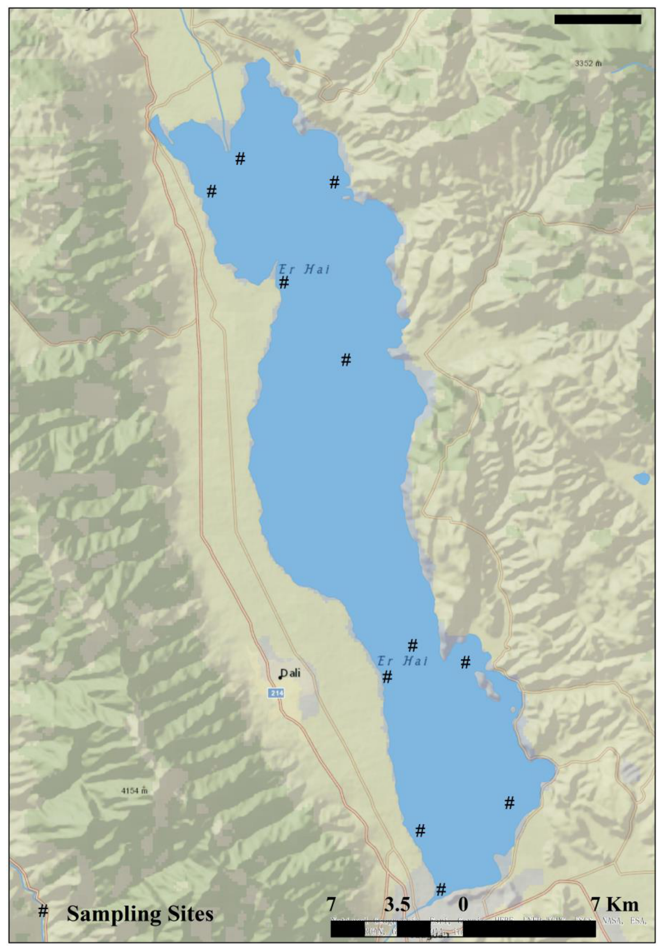
Figure 2.
Monthly variation in environmental conditions and bulk water-quality parameters in Lake Erhai from November 2023 to October 2024. (a) Heatmap of monthly z-scores for water temperature, TN, TP, NH4+-N, NO3−-N, PO43−-P, Chl-a and DOC. (b) Monthly means of Chl-a, DOC and water temperature.
Figure 2.
Monthly variation in environmental conditions and bulk water-quality parameters in Lake Erhai from November 2023 to October 2024. (a) Heatmap of monthly z-scores for water temperature, TN, TP, NH4+-N, NO3−-N, PO43−-P, Chl-a and DOC. (b) Monthly means of Chl-a, DOC and water temperature.
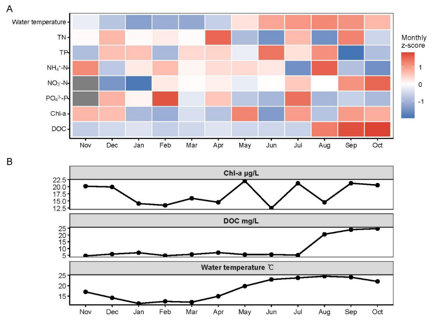
Figure 3.
Principal component analysis (PCA) of the environmental variables. (a) Site-level scores on the first two environmental principal components, coloured by sampling month, with dashed ellipses outlining the monthly distributions. (b) Variable loadings on environmental PC1 and PC2. (c) Trajectory of monthly mean environmental PC scores through the annual cycle. Values in parentheses give the variance explained by each axis.
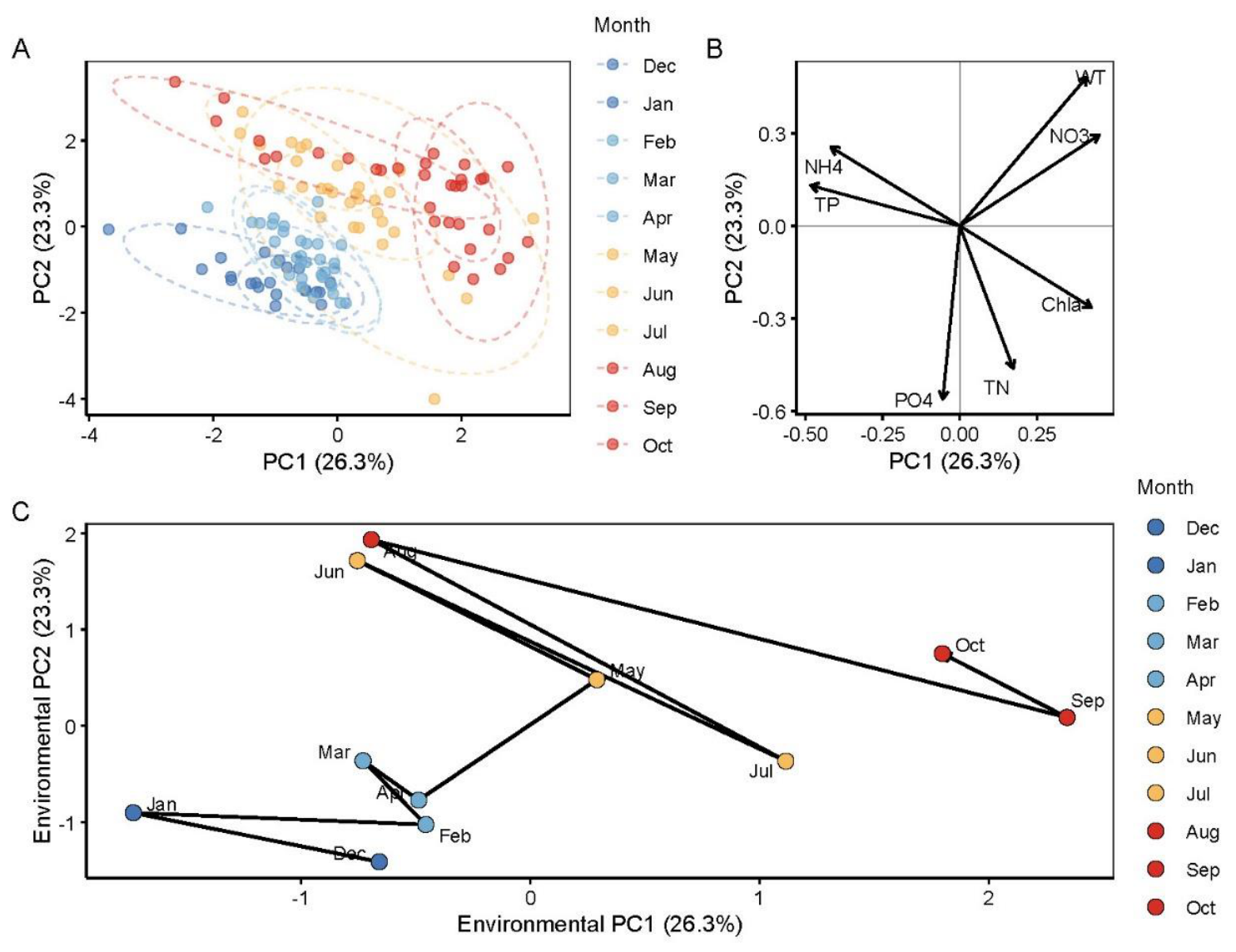
Figure 4.
Chl-a dynamics and its conditional associations with inorganic nutrients and water temperature. (a) Monthly distribution of Chl-a at the 11 sampling sites (box plots with individual observations; black dots indicate monthly means). (b–d) Partial effects of DIN (b), DIP (c) and water temperature (d) on log(1+Chl-a) estimated from the full model controlling for month and sampling location; shaded bands denote 95% confidence intervals.
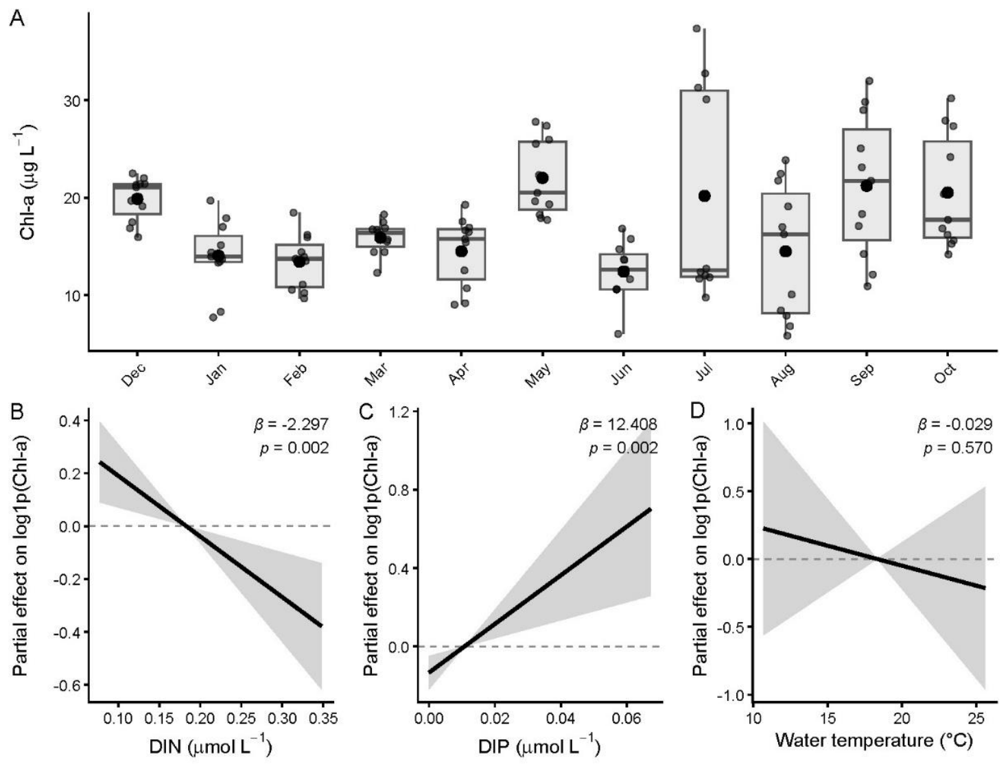
Figure 5.
Late-season accumulation of DOC. (a) Monthly mean DOC concentration, with the August–October high-DOC regime shaded. (b) Mean log(1+DOC) for the late-season regime (August–October) and for the remaining months. (c) Relationship between log(1+Chl-a) and log(1+DOC). (d) Relationship between water temperature and log(1+DOC); grey symbols denote months outside the August–October regime and red symbols denote the August–October regime.
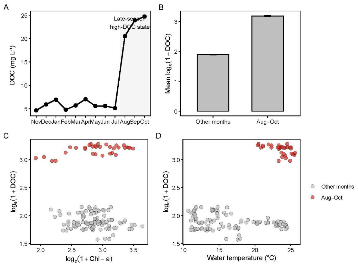
Figure 6.
Principal component analysis of DOM quantity and optical properties. (a) Site-level scores on the first two DOM principal components, coloured by sampling month. (b) Variable loadings on DOM PC1 and PC2. (c) Trajectory of monthly mean DOM PC scores. (d) Monthly variation in BIX, FI and SUVA254. Values in parentheses give the variance explained by each axis.
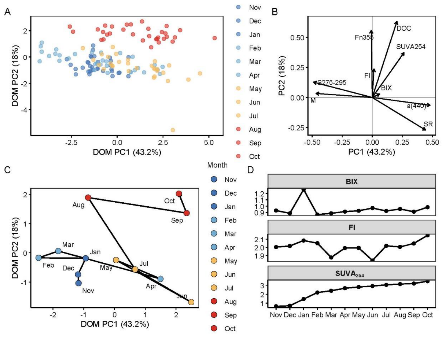
Figure 7.
Asynchronous temporal trajectories of the bulk environmental state and DOM composition. (a) Coupled trajectory of monthly mean environmental PC1 and DOM PC1 scores. (b) Euclidean distances between consecutive monthly states for DOM composition (solid line) and for the bulk environmental variables (dashed line). (c) Relationship between environmental and DOM transition distances (Spearman r = 0.382, p = 0.28); the blue line shows the linear fit and the shaded band the 95% confidence interval.
Disclaimer/Publisher’s Note: The statements, opinions and data contained in all publications are solely those of the individual author(s) and contributor(s) and not of MDPI and/or the editor(s). MDPI and/or the editor(s) disclaim responsibility for any injury to people or property resulting from any ideas, methods, instructions or products referred to in the content. |
© 2026 by the authors. Licensee MDPI, Basel, Switzerland. This article is an open access article distributed under the terms and conditions of the Creative Commons Attribution (CC BY) license (http://creativecommons.org/licenses/by/4.0/).
Copyright: This open access article is published under a Creative Commons CC BY 4.0 license, which permit the free download, distribution, and reuse, provided that the author and preprint are cited in any reuse.