

Submitted:
19 October 2026
Posted:
20 October 2026
You are already at the latest version
Abstract
The paper deals with the development of a model-based optimization framework for the design of power management strategies of a lightweight compound helicopter UAV equipped with hybrid propulsion, with focus on the transition manoeuvres from cruise to hover. A high-fidelity multi-physics model of the hybrid propulsion system, composed of a combustion-engine connected to a nose propeller for forward flight phases, and two permanent magnets synchronous machines driving variable-pitch main and tail rotors to provide control during vertical flight phases, is firstly presented. In the model, the aerodynamic loads are obtained by applying an advanced BEMT-based code, including post-stall, tip-loss and low-Reynolds corrections, as well as QPROP-derived induced velocities. The dynamics of the electric machines is simulated via equivalent bi-phase model taking account of the Field-Oriented Control technique used for the three-phase electronic commutation. As a first step of the dynamic optimization process, a so-called fixed-point optimization is obtained, by finding the speeds and blade pitch angles of the rotors that minimize the steady-state electrical power absorption in vertical flight phases. To compare the optimization results with a baseline, a reference manoeuvre is then defined, in which the rotors speeds are ramped from standstill to the optimal fixed-point values, while the blade pitch angles are dynamically adjusted to ensure the UAV vertical equilibrium. Subsequently, a constrained optimization problem is applied by using the high-fidelity model, determining the main rotor commands that minimize the power consumption during transition. Finally, the robustness of the system performances against parameter uncertainties is statistically characterized via Monte Carlo simulations. The results demonstrate the effectiveness of the proposed strategies in reducing the energy consumption and in improving the overall performances with respect to a baseline manoeuvre, highlighting the effectiveness of model-based optimization for the power management design of novel UAV platforms.
Keywords:
compound helicopter
; VTOL UAV
; hybrid-electric propulsion
; BEMT
; model-based optimization
; uncertainty quantification
; Monte Carlo analysis
1. Introduction
The electrification of aerial propulsion systems is one of today’s central lines of development in the aeronautical world, driven by the need to reduce emissions, noise, thermal signature and to simplify the maintenance process. For Unmanned Aerial Vehicles (UAVs) featuring Vertical Take-off and Landing (VTOL) capabilities, the driver is also operational, since electric drives offer precise and fast torque control that is crucial for their safe operation, especially for those with a convertible configuration. Up to date, the main roadblock hindering the electrification process is power density storage technology, since batteries specific energy remains roughly two orders of magnitude below that of hydrocarbon fuels, so that full-electric solutions are today still confined to short-endurance missions or Advanced Air Mobility applications. The hybrid-electric propulsion, in which a thermal engine and an electrical machine cooperate, is the pragmatic compromise that preserves endurance while retaining controllability and environmental advantages of electric drives [1,2]. Its application to lightweight UAVs has been addressed for the retrofit of system architectures [3] as well as for on-board power management [4].
A second line of development concerns the aero-mechanical configuration. Blending the vertical-flight capability of the helicopter with the cruise efficiency of the fixed wing removes the need for prepared runways without paying the full endurance penalty of a rotorcraft, and compound configurations, in which a wing unloads the rotor in forward flight and a separate propulsor provides thrust, have been studied extensively for their performance and aeromechanics [5,6,7]. The project VERTIGO, funded by Italian public institutions, pursues this combination by developing a lightweight (mass from 70 to 150 kg) copter-plane UAV behaving as a gyrodyne during vertical flight, with electrically-drive tilting main rotor and anti-torque tail rotor, and operating as an airplane during cruise, with a fixed wing and a pusher propeller driven by a Wankel engine. Clearly, a transition between these two regimes is to be managed in the conversion from cruise to hover and vice versa. A complex manoeuvre is to operated, in which the UAV decelerates (thus loosing the motion control via fixed wings and aerodynamic movables) and the vertical and tail rotors are driven from standstill to speeds that assures the motion control in helicopter mode. The whole transition must be executed by holding altitude and maintaining the commands within acceptable limits.
In literature, the design of transition manoeuvres has been mainly addressed as a trajectory-optimization problem: direct transcription and collocation for tilt-wing vehicles [8,9], optimal-control formulations of the transition strategy [10,11], gradient-based minimum-power trim across the transition corridor [12], mode-scheduling strategies for tilt-rotor UAVs [13], coupled optimization of design and trajectory [14], and planning validated in flight [15]. In all of these works the propulsion system enters as a simple source of thrust, so that the propulsion/actuation dynamics (i.e. current and speed responses, sensor errors effects) as well as the structural compliance is disregarded. Other authors focus their attention on the energy management of hybrid-electric platforms, classifying the strategies as rule-based, optimization-based or learning-based and solving the power split over a mission profile, for instance by dynamic programming [16], or building high-fidelity propulsion system models [17]. In those works, the electric drives are modelled in detail, but power management relies on quasi-static distribution of energy among sources over a mission, and the question of what the rotor commands should be inside a transient is not posed. The hybrid propulsion system of the VERTIGO UAV has been characterized in terms of performances in [18], by using a reduced-order multi-physics model, in which the aerodynamic loads on rotors are referred to a single speed value, the dynamics of the electric machines is simplified with equivalent mono-phase models, and the transition dynamics and its optimization are essentially disregarded. To bridge the gap, a high-fidelity multi-physics model is needed, in which the aerodynamic, electrical, structural and control domains coexist, so that the transition manoeuvre can be firstly designed and then verified against uncertainties. Concerning the aerodynamic domain, the Blade Element Momentum Theory (BEMT), extended with Reynolds-dependent airfoil data, post-stall models and improved tip-loss corrections, can be effectively used to predict rotor thrust and torque without excessive computational burden [19,20,21,22]. On the electrical drive side, nonlinear models taking into account of the electronic commutation technique should be included to characterize performance and robustness [23,24,25,26].
The objective of this work is thus to design and optimize the power-management strategy used for the cruise-to-hover (and vice versa) transition of the hybrid-propulsion compound helicopter UAV developed in the project VERTIGO, aiming to determine the combination of speed, collective pitch and tilt angle of the vertical rotor that guarantees equilibrium during the manoeuvre while minimizing the electrical energy consumption.
The main scientific contributions of the paper are:
- the development of a high-fidelity multi-physics model of the propulsion system, by integrating BEMT-derived rotor maps, nonlinear dynamics of the electrical drives, dynamics of the pitch and tilt actuators, structural compliance of the vertical rotor blades, and sensor errors
-
the development of a scalable and generalized optimization methodology based on three steps:
- preliminary selection of a candidate optimal manoeuvre through the closed-form solution of a reduced-order nonlinear ODE problem representing the transition dynamics of a point-mass model;
- demonstration that the resulting optimum is invariant with respect to code parameters (three unrelated families of tilt angle laws are used, all converging the same result);
- validation of the optimum with the high-fidelity multi-physics model;
- characterization of robustness of the optimum against uncertainties of model parameters.
The paper is organized as follows. Section 2 describes the vehicle and its hybrid propulsion system, the aerodynamic, electrical, control and structural models that compose the simulation environment, the baseline transition manoeuvre, the closed-form reduction and the uncertainty campaign. Section 3 reports the validation of the simulation environment, the fixed-point optimization results, the baseline manoeuvre, the outcome of the closed-form search, its validation on the nonlinear model and the robustness analysis. Section 4 discusses the results and the limits of the study, and Section 5 draws the conclusions and proposes future developments of the research.
2. Materials and Methods
2.1. System Description
The VERTIGO UAV is developed for prolonged surveillance missions, combining a hybrid aero-mechanical architecture with a hybrid thermal-electric propulsion system. From an aero-mechanical standpoint the vehicle is a compound helicopter: during vertical flight it behaves as a gyrodyne, where a tilting two-bladed main rotor provides lift and longitudinal/lateral control while a ducted tail rotor with a fenestron design provides the anti-torque and yaw functions; while during horizontal flight it behaves as a conventional fixed-wing aircraft, where the wing provides the necessary lift to balance the weight, a pusher propeller driven by an internal combustion engine provides thrust, and the main rotor is braked and feathered with its blades aligned with the longitudinal axis. Figure 1 shows the conceptual three-view drawings of VERTIGO aircraft aerodynamic configuration while Table 1 summarizes the operational requirements [27].
The prolonged stationary surveillance mission has been considered the reference for this work, Table 2. It can be noted that, since the two electrically-driven rotors are active for about 75 % of the mission duration, they dominate the UAV energy budget.
The VERTIGO hybrid propulsion system (HPS), Figure 2, is made of:
- a two-bladed tilting vertical rotor (TVR) with variable collective pitch, of radius 2.5 m and uniform chord 0.16 m, whose axis direction is controlled by two electromechanical servo-actuators. The TVR provides vertical thrust during vertical flight and, by tilting the thrust vector, the longitudinal acceleration and deceleration needed to convert between hover and horizontal flight. A one-way sprag clutch in its mechanical transmission disconnects the rotor from its motor in the event of a motor failure, enabling autorotation;
- a two-bladed ducted tail rotor (TR) with variable collective pitch providing anti-torque and yaw control during vertical flight;
- a Wankel internal combustion engine (WICE) driving a variable-pitch pusher propeller through a clutch and an adjustable-ratio gearbox, equipped with an electric turbocharger, liquid cooling and two electric generators rated 22 kW continuous and 30 kW peak;
- a power distribution unit feeding a DC bus whose voltage can be selected among 48, 96, 144 and 192 V;
- two three-phase permanent-magnet synchronous machines (PMSMs) driving the TVR and the TR, each with its own electronic power unit, electronic control unit built around a six-MOSFET power converter, and thermal management system;
- a power management unit (PMU) that distributes the generated electrical power among the users according to the flight phase.
2.2. Model of the Aerodynamic Loads on Rotors
The following sections detail the analytical model developed for the estimation of the aerodynamic loads on the rotors and the code implementation developed for the computation of the Look up tables used in the non-linear dynamic simulation models. At the design stage addressed by this work, both the geometry and the airfoils of the main rotor have been frozen. The tail rotor, however, is defined only by its function and its envelope: neither its blade geometry nor its airfoil has been frozen. Its performance maps therefore cannot be computed directly. For this reason, a parametric identification problem has been solved by identifying the geometry of an equivalent rotor against the performance database of a commercial propeller. Details of the identification are omitted for the sake of brevity.
2.2.1. BEMT/QPROP Formulation
At a generic rotor’s blade station of radius r the local velocity triangle defines the geometric, effective and induced incidences through Eq. (1)
where θ is the local pitch angle, ϕ the inflow angle due to axial velocity, α the geometric incidence, αe the effective incidence and αi the induced incidence, U∞ the asymptotic axial velocity and Ω the rotational speed (Figure 3).
The elementary lift and drag acting on the blade element follow from the sectional aerodynamic coefficients, with the assumption of a linear relationship between coefficient of lift CL and effective incidence αe and a parabolic polar, i.e.
in which c is the local chord, Ve the effective velocity acting on the blade section and B the number of blades composing the rotor. Eq. (2) can be further expanded by expressing αi as a function of αe, θ, U∞ and Ω and expressing via the Pythagorean theorem:
Projecting these elementary actions onto the rotor axis and onto the disc plane gives the elementary thrust and in-plane force,
The second relation of the theory comes from momentum conservation applied to the annulus swept by the blade element, which for an axial flow gives [28,29,30]:
dT = 2ρ(U∞ + wcosϕ)wcosϕdAR = 4πρ(U∞ + wcosϕ)wcosϕr dr = fT2(w, r)
Equating the blade-element and momentum expressions of the elementary thrust closes the problem at each station. Two implementations were developed. The simplified one solves the resulting scalar equation for the induced incidence at each station. The advanced one follows the formulation proposed by Drela for QPROP [31]: it retains both the axial and the tangential induced velocity components, does not assume a small inflow angle, and solves at each station the coupled system:
by Newton iteration on a single angle, where Γ(r) is the bound circulation, λw the local wake advance ratio and F the tip-loss factor and wa is the axial component of the induced velocity, wa = wcosϕ. The reader shall note that the second term of the second equation of the system (6) is equivalent to the thrust prediction of the momentum theory, term fT2 expressed by Eq. (5). The swirl component and the large-angle formulation matters for this application, because the rotor operates at low advance ratio and, during the transition, at collective settings close to the stall boundary.
Several simplified assumptions stand behind the implementation of the BEMT code discussed in the following sections:
- -
- Blade flapping is neglected.
- -
- Rotor inflow due to aircraft advancing velocity is neglected.
- -
- Dynamic stall on the retreating blades is neglected.
- -
- Compressibility effects on the advancing blades are neglected.
- -
- The effect of the flow velocity component parallel to the blade is neglected (only axial and tangential components are considered).
2.2.2. Code Implementation and BEMT Corrections
The software developed for this work features an iterative non-linear solver with a two-pass strategy approach. The solver first executes a run from the blade tip to the blade root because the local high speed at the root ensures the computed local incidence to lie within the stall boundaries and thus guarantees a feasible physical solution. As a second step, the code uses, sweeping from the hub to the tip, the pre-computed values as initial guess to refine the solution. This choice prevents near-hub stalled solutions to propagate towards the rest of the blade.
From a geometrical standpoint, the code assumes linear distribution of profile chord and twist. To increase physical fidelity of the prediction, with a better characterization of the blade behavior near its root, the software distinguishes between hub and blade. Hub is treated as a bluff body, with zero lift, akin to the flat plate model perpendicular to the airflow, which only generates aerodynamic drag:
where is the drag coefficient of the hub and hhub is its section height (assumed constant spanwise). The aerodynamic drag generated by the hub is then projected in its axial and transversal components. Furthermore, three sources of nonlinearity are modelled in the implementation:
- sectional coefficients are read from tabulated airfoil polars [32] as functions of both the effective incidence and the local Reynolds number.
- tip losses are accounted for by means of two different strategies. In the simplified BEMT, αi, αe and CL are linearly interpolated from their respective values at the station located at
to zero, whereas the aerodynamic coefficient CD is interpolated to the profile zero lift value CD0. Conversely, in the advanced QPROP based implementation, the tip loss is accounted through a Prandtl factor [31]:
written in a regularized form, so that the solution remains well posed in vertical descent, where the induced flow reverses sign and the rotor approaches the vortex ring state.
- post-stall behaviour is modelled with the Viterna extension of the polars [33], blended with the measured polar through a smooth weighting function:
CL = (1 − β)CL,pol + βCL,vit
Figure 4 shows the comparison between the simplified and advanced BEMT implementations applied to the NACA0006 profile of the main rotor in hover for the same produced thrust.
As it can be noted, the two implementations exhibit a substantial agreement in the distributions of angles of attack and elementary forces per unit span except for the sections near the blade tip where 3D effects such as vortex shedding are non-negligible. Table 3 summarizes the comparison of performance prediction for the hover condition. Once more, the two implementation appear in substantial agreement for the collective angle required to produce a given thrust but as expected the simplified BEMT underestimate the Torque and thus the required power to produce such thrust by a 5% margin.
This is clearly due to the assumptions introduced in the simplified implementation, namely: the absence of the swirl component of flow velocity, an aerodynamic model with constant coefficients rather than a parametrization with Re and the fact that tip effects are not properly taken into account but a simple interpolation of the coefficient is carried out. For this reason, the advanced BEMT has been selected to compute rotor performance maps. The optimized code, despite a computational cost about one order of magnitude higher with respect to the simplified implementation, achieves convergence for a single condition in less than 1 s, allowing the creation of tables composed of hundreds of operating points in few minutes.
The BEMT code is then run over a grid of collective pitch angles and rotational speeds for each of the three vertical flight conditions, and the results are expressed as thrust and torque coefficients as expressed by Eq. (10),(11):
Figure 5 and Figure 6 show CT and CQ for the main rotor in hover flight. Two main physical features can be inferred: first, both coefficients are roughly independent from speed; second, they are essentially linear with the collective pitch angle. This means that thrust and torque are essentially quadratic in Ω and linear in θ, which makes the inverse problem described in Section 2.6.2 straightforward to solve.
2.3. Fixed-Point Optimization in Vertical Flight
The redundancy between collective pitch and rotational speed identified in Section 2.1 is resolved, for the steady vertical flight phases (hover, vertical take-off and vertical landing), by solving a constrained optimization problem. The cost is the total mechanical power absorbed by the two rotors and the decision variables are the collective pitch and the rotational speed of each of them:
subject to box constraints on the four decision variables and to two nonlinear equality constraints, which impose vertical equilibrium, that is that the main-rotor thrust balance the weight, and yaw equilibrium, that is that the tail-rotor thrust times the tail arm balance the main-rotor torque.
The bounds of Table 4 come from the hardware. The collective pitch ranges are set by the pitch mechanisms. The upper bound on rotor speed follows from the maximum speed of the electric machine, itself fixed by the bus voltage and the machine electrical constant through the transmission ratio; the lower bound is the minimum speed at which the rotor can still produce the thrust required for equilibrium at maximum collective. This last quantity, referred to in the following as the authority speed, plays a central role in the transition manoeuvre, because it is the speed below which the rotor cannot sustain the vehicle whatever the pitch command.
2.4. Model of the Electrical Machines
2.4.1. Electrical Dynamics and Torque Generation
Each rotor is driven by a three-phase permanent-magnet synchronous machine. For a machine with sinusoidal back electromotive force the phase voltages obey [34]:
where Ra,b,c, Ia,b,c, La,b,c are the phase Resistance, Current and Inductance respectively and the back electromotive forces ea,b,c are proportional to the rotor flux linkage λm and to the electrical angular speed and are mutually shifted by one third of a period,
This three-phase description is not convenient for control design, because its coefficients depend on the rotor position. It is therefore projected onto a frame rotating with the rotor by the combined Clarke and Park transformation [35], written here in the power-invariant orthogonal form so that its inverse coincides with its transpose:
Applying it to the phase equations and neglecting the homopolar component gives the reduced model in the direct and quadrature axes (indicated by subscripts d and q respectively):
which is completed by the expressions of the active and reactive electrical power and of the electromagnetic torque,
The two machines driving the main and the tail rotors have been selected from a manufacturer catalogue [36,37] on the basis of the power requirements established in Section 2.3. Their parameters are collected in Table 5. The phase resistance (not provided in the datasheet) is estimated from the loss budget declared in the datasheet, by attributing a prescribed fraction of the total losses to the Joule term, and the phase inductance from the requirement that the electrical pole lie well above the current-loop bandwidth. The torque constant is reported by the manufacturer per unit root-mean-square phase current; the value entering the direct-quadrature model follows from the power-invariant transformation and is therefore smaller by a factor of the square root of three. The electrical drive models have been validated against the load curves provided by the manufacturer [36,37], which give the absorbed electrical power as a function of speed for different values of constant external torque. Closed loop simulations have been carried out with the motors subjected to the same constant torque values along a speed ramp slow enough for the electrical and mechanical transients to be negligible, so that a quasi-static behavior can be assumed.
2.4.2. Closed-Loop Control Design
The speed of each machine is regulated by the classical field-oriented strategy [35] whose architecture is depicted in Figure 7, comprising an inner current loop, closed on the quadrature and direct currents, nested inside an outer speed loop, both with proportional-integral regulators. The direct-current reference is held at zero, so that the whole stator current produces torque.
Taking the voltage cleared of the back electromotive force as the input (), the equivalent single-phase model of Section 2.4 gives a first-order current plant,
and the regulator is chosen proportional-integral,
where evidently, u(s) and e(s) are the control and error signals respectively, are the integral and proportional gains respectively and their ratio zi is selected to cancel the electrical pole of the plant. The open-loop transfer function then reduces to a pure integrator, and the closed loop to a first order whose pole is set directly by the proportional gain,
so that assigning the required current bandwidth fixes the proportional gain as the product of the phase inductance and the bandwidth, and the integral gain follows as the product of the phase resistance and the same bandwidth. A current bandwidth of 30 Hz has been specified for both machines.
The back electromotive force, which the pole cancellation deliberately does not try to reject, is reinstated downstream of the regulator by a feed-forward term computed from the measured speed; the proportional-integral regulator is thereby left with the sole task of rejecting disturbances. An anti-windup scheme with a tracking time constant of 10 ms prevents the integral term from drifting when the voltage command saturates.
The outer loop is designed on the torque balance of the shaft, which relates the speed to the electromagnetic torque through the combined inertia of machine and rotor and the viscous friction, the aerodynamic load being treated as a torque disturbance,
The same pole-cancellation strategy is applied, and a speed bandwidth of 3 Hz is obtained.
2.5. Model of the UAV Motion
2.5.1. Translation Dynamics
The UAV translation motion is described by a point-mass model, disregarding attitude and yaw dynamics. Under the assumption of collinearity between flight speed and forward propeller thrust, and by assuming straight-and-levelled flight, we have:
where u and w are the longitudinal and vertical velocity components, m the vehicle mass, Δ the tilt angle of the main rotor, TMR represents main-rotor thrust, D the aerodynamic drag, Lw fixed-wing Lift and Tfp is pusher propeller thrust. The manoeuvre begins in trimmed level flight at cruise speed, so the initial vertical velocity is zero.
The load transfer between wing and rotor, which is the physical heart of the manoeuvre, is derived from the speed dependence of the wing lift. In trimmed level flight at cruise speed the wing carries the whole aircraft weight, hence:
where clearly S represent the wetted surface area of the fixed wing, CL is the Lift coefficient (assumed constant throughout the transition manoeuvre), ρ indicates air density, so that as the vehicle decelerates the wing sheds lift in proportion to the square of the speed, and the main rotor must take up the difference. The drag is modelled in the same quadratic form as:
where the term CD denotes the drag coefficient.
During the transition manoeuvre, the collective pitch of the main rotor must be regulated to produce the thrust required for vertical equilibrium while the rotor speed increases and the UAV longitudinal speed decreases,
where Δ is the main rotor tilt angle Given the rotor speed, the thrust is biunivocal with pitch (Figure 5), so that
This inversion is performed at every integration step by a dedicated function block. It is inexpensive because of the structure of the maps noted in Section 2.2.2: at fixed rotor speed the thrust is monotone in the collective, so the inverse exists and is single-valued, and the near-linearity of the map makes the search converge in very few iterations.
It is worth noting that this collective law is purely feed-forward. There is no altitude or vertical-speed feedback anywhere in the model, and no regulator on the collective. This was done intentionally because the purpose of the model is to verify whether a scheduled manoeuvre is flyable, and a feedback loop on altitude would mask a defective schedule by correcting it. Any altitude excursion reported in Section 3 is therefore an actual measure of the error committed by the open-loop schedule.
2.5.2. Actuation Dynamics and Lead-Lag Compensation
Both collective and tilt actuators are modelled as first-order lags with a bandwidth of 3 Hz, which is representative of the electromechanical pitch and tilt mechanisms of this class of vehicles. The introduction of a first-order lag causes a drop in altitude. During the deceleration phase indeed, the required collective grows continuously, and a first-order lag tracking a ramp exhibits a steady velocity error:
where τ is the time constant and θ the collective rate. The delivered collective therefore remains persistently below the scheduled one, the rotor produces less thrust than required for equilibrium, and the vehicle slowly loses altitude.
A simple feed-forward inversion is chosen to mitigate the problem. A lead pre-compensator is placed on the scheduled collective, upstream of the actuator,
whose zero cancels the actuator pole, so that the cascade of compensator and actuator behaves as a first-order lag of time constant reduced by the factor N. With the actuator time constant set by the 3 Hz bandwidth and N = 10, the residual bandwidth seen by the collective schedule is 30 Hz, and the drop in altitude disappears.
2.5.3. Yaw Dynamics
To obtain the yaw balance, the torque applied on the main rotor must be balanced by an anti-torque action, given by tail rotor thrust. The collective pitch of the tail rotor is therefore commanded by a PID regulator acting on the heading error:
The UAV yaw dynamics is described by
where JZ is vehicle moment of inertia around its z body axis, ψ is Euler’s yaw angle, while QM and QT are the moments generated by main rotor and tail rotor respectively. By linearizing the tail rotor thrust at a given speed, we obtain:
where l is the yaw control arm (distance between tail rotor hub and UAV centre of grafvity), kt is the thrust slope coefficient with respect to pitch. If Eq. (29) and Eq. (31) are combined and the Lapalace transform is applied, we have:
A pole-placement technique is finally used to define the regulator gains, up to obtain:
- a real pole at λ = −6 rad/s
- two well-damped complex-conjugated poles having
- damping factor ζ = 0.7 and
- natural undamped pulsation ωn = 1.5 rad/s
As a result, the three regulator gains of the yaw control system are:
2.5.4. Structural Compliance of the Main Rotor Blades
During the rotation, all blades exhibit flexural strain, and the entity and the effects of this strain increase with blade length. For the main rotor, the flexural deflection under load can significantly vary the local incidence of the incoming flow. A simplified representation of this effect is included in the UAV HPS model, for which the blade is considered as a rigid body hinged on an elastic root restraint, enabling the flapping motion. The resulting dynamics is,
The blade inertia follows from the blade mass and radius, the stiffness is assumed from typical values found in literature for similar blade geometry, and the damping is assigned a ratio of 0.1 with respect to the resulting undamped natural frequency. The coupling back onto the aerodynamics is the essential part: the flapping velocity changes the axial component of the relative velocity at the blade section, hence the incidence, by
which is subtracted from the commanded collective before the aerodynamic maps are interrogated. The resulting first bending mode lies near 40 Hz, well separated from the manoeuvre timescale but not from the actuation bandwidth, which is why it is worth retaining in a model intended to assess an actuation system.
2.5.5. Sensor Noise
To increase the physical representation as well as to permit disturbance rejection analysis, the measurement noise is also introduced in the UAV HPS model. A normally-distributed noise, sampled at 1 kHz, is thus injected on both rotor speed feedbacks of electrical machines, and on the collective pitch and tilt commands. The standard deviation has been set as a fixed fraction of the full scale of the channel, so that the signal-to-noise ratio is uniform across channels of very different physical magnitude, rather than tuning each independently.
2.6. High-Fidelity Multi-Physics Model of the HPS
The model sections described in previous paragraphs have been integrated by obtaining a high-fidelity model of the hybrid propulsion system, implemented in MATLAB/Simulink and numerically solved via Runge-Kutta method, using a fixed step of 1 ms, Figure 8.
The model thus contains the rotor maps of Section 2.2 as lookup tables, the electrical machine models of Section 2.4 with the control laws of Section 2.5, the flight mechanics described below, the pitch and tilt actuators with their dynamics, a simplified representation of the blade structural response, sensor noise, and the yaw stabilisation loop.
2.7. Baseline Transition Manoeuvre Definition
A reference manoeuvre, to be used as baseline for comparing optimization results, is defined so that:
- the manoeuvre starts from level flight at cruise speed and constant altitude;
- altitude is held constant throughout, and vertical equilibrium must be satisfied at every instant;
- the rotor is accelerated along a ramp, up to the authority speed;
- while the rotor accelerates it remains unloaded, and the drag is balanced by the pusher propeller;
- once the authority speed is reached, the pusher propeller no longer produces thrust, the rotor progressively begins to take up the lift shed by the wing, and it is tilted backwards so that the longitudinal component of its thrust decelerates the vehicle;
Imposing altitude hold and assuming that the pusher thrust vanishes instantaneously at the authority speed, the system (22) collapses into:
from which the tilt angle and the rotor thrust required for equilibrium are determined uniquely, instant by instant, by the current speed and the deceleration being demanded,
The baseline is obtained by demanding a constant deceleration throughout the entire manoeuvre equal to the deceleration that the vehicle would experience under its own drag alone at the instant that the pusher propeller is feathered:
Substituting it in the previous relations gives
Now, the model developed and the tilt angle turns out to be constant. Holding the tilt at this value makes the two speed-dependent terms of the longitudinal balance cancel identically, so the deceleration is indeed exactly constant for the whole manoeuvre: the constant-tilt manoeuvre and the constant-deceleration manoeuvre are the same manoeuvre. With the VERTIGO parameters the tilt angle is approximately 4 degrees and the deceleration is ≈ 0.7 m/s², so that the vehicle takes 58.3 s and 1166 m to come to a stop from cruise speed.
2.8. Closed-Form Reduction and Optimization Problem
A constrained optimization problem has been formulated to address the question of which tilt law minimizes the energy of the manoeuvre. A reduced model, evaluated in microseconds is employed to search exhaustively on a large population, while the full non-linear model is exploited for the validation of the winner solution.
The reduction rests on one observation: by expressing the tilt angle as a function of flight speed, time can be factored out of the problem, and the state vector can be formulated solely as a function of flight speed. Vertical equilibrium fixes the rotor thrust, and the longitudinal balance fixes the acceleration, both algebraically can be expressed as:
At a given fixed rotation speed, the required main-rotor mechanical power then immediately follows from the thrust through a one-dimensional table. Because thrust is monotone in collective at fixed speed, this table is invertible, and reading it returns both the power and the collective required.
The metrics of the manoeuvre are obtained by trapezoidal quadrature in the speed domain. Since the speed decreases monotonically, it can be used as the independent variable, and the time, distance and energy follow from:
so that evaluating a candidate tilt law costs one pass over a speed grid of a few hundred points.
A candidate is admissible only if it produces a deceleration for each point (a(k) < 0 ∀ k = 0,…,n), if the thrust it demands is within what the rotor can deliver, and if the tilt and collective it requires stay inside the actuation limits of 20 and 12 degrees respectively.
The objective combines two competing contributions, the overall electrical energy required for the manoeuvre and the peak power demanded of the bus, each normalised by the minimum observed over the whole population:
where wE represents the energy weight. Three independent parametrizations families of the tilt law were investigated:
- (a)
- a shape-preserving piecewise cubic interpolant through freely placed set-points, explored by a Monte Carlo sample of one million candidates;
- (b)
- a one-parameter hyperbolic-tangent shaped class;
δ=min(max( δ*tanh(3u),0 ), δmax)
- (c) a double-exponential function with five parameters fitted to the optimum of the first via a nonlinear least-square approach:
where the five estimated parameters are the two exponential amplitudes A1, A2 the two time constants τ1, τ2 and the lag term Δu which dictates the temporal separation between the two exponentials.
Finally, in each case the best sample is refined by an interior-point gradient search.
2.9. Uncertainty-Quantification via Monte Carlo Simulations
An Uncertainty-Quantification (UQ) campaign was carried out to investigate how parameter uncertainty propagates through the full nonlinear model and to attribute the resulting dispersion of the performance metrics to its sources.
Three uncertain parameters are considered:
- -
- phase resistance of the main machine.
- -
- torque constant.
- -
- an additive bias on the main-rotor torque map.
Each is treated as normally distributed about its nominal value, with a standard deviation equal to one eighth of the reference; the torque bias has zero mean and is scaled on the hover torque. Only the main drivetrain is perturbed.
The design is a full factorial grid of sixty levels per parameter, that is 216,000 nonlinear simulations. A tensor grid is used to allow for variance decomposition. A grid is, however, a poor sampler for the shape of the output distributions, since it contains only sixty distinct values per input; an independent Latin-hypercube sample of three thousand runs is therefore added for the distribution estimates alone, and doubles as a cross-check that the two designs agree. The metric chosen are: peak total electrical power, cumulative electrical energy, maximum altitude excursion, ground distance covered, and peak blade elastic response.
The attribution of the dispersion is made through first-order Sobol indices, which measure the fraction of the output variance that would be removed if one input were known exactly:
they computed here directly from the tensor grid by conditional averaging.
3. Results
3.1. Rotor Operating Points for Minimum Power in Vertical Flight
Figure 9 shows main rotor and tail rotor required power for the three vertical flight conditions comparing baseline and optimized, while Figure 10 shows relative changes with respect to baseline operating points (preliminary design phase). The optimizer moves the main rotor in the same direction in all three conditions: the rotational speed is reduced by about 19 % and the collective pitch increased by about 40 %, so that the same thrust is produced with a higher blade loading at a lower tip speed. The main-rotor torque rises by about 14 %, but the power, falls: by 7.0 % in hover, from 12.5 to 11.63 kW. Because the higher torque must be balanced by the tail, the tail thrust and hence required power rise, and the total mechanical power of the two rotors falls by 5.5 % in hover, from 13.28 to 12.55 kW. A reduction of 0.73 kW in hover may look modest, but the reference mission of Table 2 includes 103 min of hover, so it amounts to about 1.25 kWh per mission; adding the vertical take-off and landing phases, in which the savings are 0.60 and 0.76 kW respectively, brings the total to about 1.31 kWh. The hover solution, 488.7 rpm and 8.68° of collective, is the state in which every transition manoeuvre of the following sections must end; the same value of rotor speed is held constant during the deceleration in the closed-form design of Section 2.8.
3.2. Baseline Transition Manoeuvre Simulation
The baseline manoeuvre described in Section 2.7 was simulated on the full nonlinear model described in Section 2.6. Figure 11 shows main rotor angular speed, collective angle and the aircraft’s flight speed. The rotor is spun up along its ramp from standstill; during the spin-up the collective sits at a slightly negative value that keeps the rotor unloaded; from the authority instant onwards it rises monotonically, with its value being updated continuously by the inverse look-up strategy discussed in Section 2.6.2, to produce the share of lift required for vertical equilibrium. The vehicle decelerates linearly, as the constant-tilt analysis predicts, and comes to rest 58.17 s after the tilt is engaged, having covered 1166 m, following the prediction of the closed-form model.
Figure 12 (a) shows the electrical powers absorbed by the two drives and their cumulative energy. The main-motor power carries a visible kink at the end of the spin-up ramp, where the inertial related torque of the rotor disappears; afterwards the signal follows the growth of the required thrust. The tail-motor power is about an order of magnitude smaller, as expected from the fixed-point results. Measured from the tilt engagement to its end, the manoeuvre absorbs 131.0 Wh of electrical energy with a peak total power of 13.53 kW. The closed-form model, which accounts for the main-rotor mechanical power only, gives 119.1 Wh and 11.71 kW; the difference is clearly explained by the presence of the tail drive and the motor/converter losses in the full, non-linear simulation model.
Figure 12 (b) documents the load transfer and the altitude hold. The wing lift and the vertical component of the rotor thrust sum to the weight throughout, ensuring vertical equilibrium of the aircraft; the rotor thrust normalised by the weight, plotted against the flight speed normalised by the cruise speed, follows the parabola predicted by the constant-tilt analysis, i.e. second equation of the system (39). The altitude excursion over the whole manoeuvre is 2.25 m, entirely attributable to the open-loop nature of the collective schedule and to the actuator lag discussed in Section 2.6.3, since no altitude feedback exists in the model, while the vertical flight speed at the end of the manoeuvre lies below 6 cm/s.
3.3. Closed-Form Optimization Results
The closed-form optimization has been performed with the three parametrizations of the tilt law on a speed grid of 400 points, with the rotor speed held at the hover optimum value (51.2 rad/s) and the energy weight factor set to we = 0.15. The following classes of tilt law functions have been defined:
- Class A: piecewise cubic interpolant passing through the free set-points (eight ones in this work), sampled one million times
- Class B: one-parameter hyperbolic tangent shaped class, where the parameter is the maximum amplitude of Δ command.
- Class C: double-exponential law expressed by Eq. (44), obtained by least-square best-fit of the optimum of Class A (a smoother law with five parameters replaces the eight set-points).
The winner of each Monte Carlo simulation has been then refined by an interior-point gradient search on the same cost. Table 6 collects the optima of the three families together with the closed-form evaluation of the baseline, all scored on the common normalization, in which the population minima of energy and peak power are 31.7 Wh and 11.67 kW.
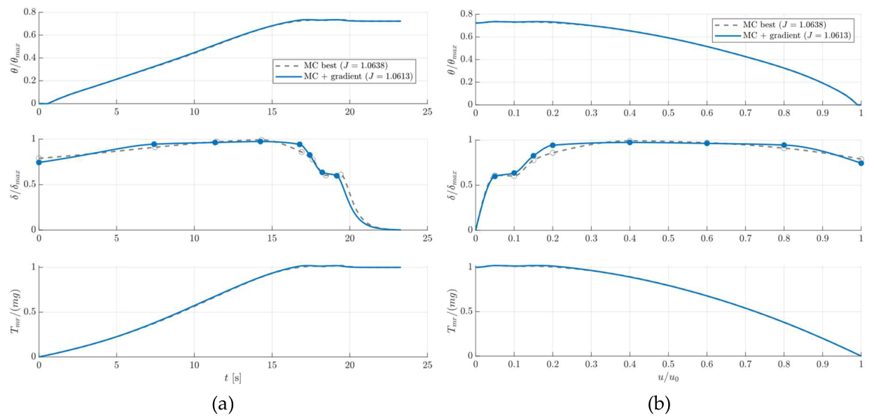
It can be pointed out that classes A and C are coherent: they differ in computational cost (by roughly four order of magnitudes), while in energy, peak power, manoeuvre length and stop time they essentially provide the same results. Class B, which is far more constrained, lands within 1.5 % of them in cost. Three unrelated parametrizations converging on the same point of the energy versus peak-power plane is strong evidence that the optimum is a property of the physics of the manoeuvre and not an artefact of the basis used to describe the tilt law. The gradient refinement, for its part, improves the Monte Carlo winner of class A only from 1.0638 to 1.0613, which indicates that a sample of one million already resolves the optimum closely, as Figure 15 shows. The second result is the size of the improvement over the baseline: the energy of the deceleration falls from 119.1 to 39.1 Wh, by 67 %, and the stop time from 58.2 to 21.0 s, by 64 %, while the peak power rises by only 2.7 %, from 11.71 to 12.03 kW.
Figure 13 shows the optimal tilt laws against the normalized speed. Their common shape is what the physics dictates: a steep tilt, between 15 and 19 degrees, is applied from cruise speed down to about ten per cent of it, so that the vehicle brakes hard while the wing still carries most of the weight and the rotor is lightly loaded; the tilt then relaxes, and is faded to zero over the last few per cent of the speed range so that the vehicle stops without reversing. The double-exponential fit of class C reads directly in these terms, with its coefficients: an amplitude of 13.6° with a characteristic speed of 2.8 % of the cruise speed, which is the fade, and a second amplitude of 5.3° engaged above 12 % of the cruise speed, which is the additional braking authority used while the wing still lifts. The baseline, by contrast, applies 4.0° throughout and lets aerodynamic drag do most of the braking, which is why it takes almost three times as long. Figure 14 gives the resulting histories in the time domain: flight speed normalized with cruise speed and distance, main-rotor mechanical power and cumulative energy. With respect to the baseline manoeuvre shown in Section 3.3, the optimized manoeuvre reach a higher power sooner, because the rotor is loaded faster, but held it for a third of the time; It is interesting to note that while families A and C exhibit a practically identical behaviour, the constant hyperbolic-tangent shaped class B optima has a slightly lower maximum tilt angle, with a steepest adjustment at the end of the manoeuvre. Because of this, the velocity profile of class B is slightly above the other two in the middle of the manoeuvre and the peak of power is slightly higher and delayed towards the end of the manoeuvre. This produces a small increase in the overall manoeuvre length, but a lower cumulative Energy required. The chosen energy-related optimization weight wE favors the minimization of the peak power over cumulative energy, hence the class B is characterized by a slightly lower objective value J* (see Table 6). Finally, Figure 15 shows the modest effect of the gradient descent refinement on the best Monte Carlo sample. As it can be noted, the refinement slightly adjusts the last setpoints close to the end of the manoeuvre by making the tilt profile reach the null final value in a smoother, slightly less steep fashion.
Figure 13.
Closed-form optima for the three families’ laws versus flight speed normalised by the cruise speed; (upper) normalized collective angle; (mid) normalized rotor tilt angle; (lower) main rotor thrust normalized with aircraft’s weight.
Figure 13.
Closed-form optima for the three families’ laws versus flight speed normalised by the cruise speed; (upper) normalized collective angle; (mid) normalized rotor tilt angle; (lower) main rotor thrust normalized with aircraft’s weight.
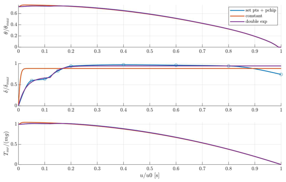
Figure 14.
Closed-form histories of the three optimal manoeuvres: (a) normalized flight speed and distance; (b) main-rotor mechanical power and cumulative energy.
Figure 14.
Closed-form histories of the three optimal manoeuvres: (a) normalized flight speed and distance; (b) main-rotor mechanical power and cumulative energy.
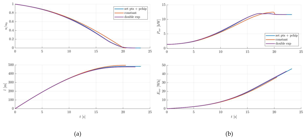
Figure 15.
Class A: comparison of best Monte Carlo sample and its gradient-based refinement; (upper) normalized collective angle; (mid) normalized rotor tilt; (lower) normalized main rotor thrust; (a) signal plotted versus time; (b) signals plotted versus normalized speed.
Figure 15.
Class A: comparison of best Monte Carlo sample and its gradient-based refinement; (upper) normalized collective angle; (mid) normalized rotor tilt; (lower) normalized main rotor thrust; (a) signal plotted versus time; (b) signals plotted versus normalized speed.
3.4. Validation of the Optimal Strategy with the High-Fidelity Model
The double-exponential law of class C was retained as the design and validated on the full nonlinear model. Its tilt profile, defined against speed, was converted into a time history through the closed-form relation between speed and time, gated to start at the authority instant, and applied open loop through the tilt actuator, with the rotor speed schedule, the collective law, the regulators, the sensor noise and the yaw loop all identical to the baseline run of Section 3.3.
Figure 16, Figure 17, Figure 18 and Figure 19 compare the nonlinear simulation with the closed-form design. The tilt delivered by the actuator follows the commanded profile with the small lag expected of a 3 Hz actuator, and the collective delivered by the inverse look-up through the lead-compensated actuator tracks its schedule closely. The flight speed and the distance covered lie on top of the closed-form prediction over the whole deceleration: the vehicle comes to rest 21.01 s after the tilt is engaged, the instant at which the closed-form schedule releases the tilt, with a residual speed of 0.13 m/s against the 0.1 m/s endpoint of the closed-form integration, having covered 479 m against 478 m. The main-rotor electrical power runs above the closed-form mechanical power by the losses of the machine and the converter, and the total electrical power adds the tail drive on top; the cumulative electrical energy of the manoeuvre, measured from the tilt engagement to the stop, is 43.6 Wh. Figure 20 shows the blade flapping angle and rate. The angle follows the rotor loading quasi-statically and the rate remains at the level of 10−3 rad/s, with the lightly damped 40 Hz mode excited only by the noise on the collective command. Within the limits of the simplified blade model of Section 2.6.4, the manoeuvre does not excite the structural degree of freedom appreciably.
Table 7 summarizes the comparison of the two manoeuvres on several metrics that the design targets, including the total electrical energy from the tilt engagement to the stop of each manoeuvre, and Figure 21 overlays their histories on a common clock. Both runs replay the identical rotor spin-up phase, so every difference between each run is confined to the braking phase. The optimized manoeuvre absorbs 43.6 Wh against 131.0 Wh, a reduction of 66.7 %, stops in 21.0 s against 58.2 s, a reduction of 63.9 %, and covers 479 m against 1166 m. whereas its peak electrical power is only 3.0 % higher, 13.93 kW against 13.53 kW. The altitude excursion is four times smaller, 0.57 m against 2.25 m, because the open-loop collective schedule has less time to accumulate error.
The last two rows of energy in Table 7 carry the central validation result of this work. The closed-form model predicts a relative energy saving of 67.1 %; the full nonlinear model delivers 66.7 %. The two models compute different physical quantities, the main-rotor mechanical energy for the case of the closed form simulation and the total electrical energy of both drives for the full non-linear simulation, and their absolute values differ accordingly, by 10 % on the baseline; yet the relative saving they predict agrees to within half a percentage point. The reduced model, characterized by a much higher computation efficiency and thus requiring fractions of the computational time required by full model, can therefore be used to investigate and design the best manoeuvre, while the full model is exploited only for verification purposes. The agreement between the two formulations is not confined to the energy: at the instants at which the closed-form schedules end, 58.16 s and 21.01 s after engagement, the nonlinear vehicle has in both cases come to rest, with residual speeds of 0.10 and 0.13 m/s against the 0.1 m/s endpoint of the closed-form integration, and the distances covered agree to better than 0.3 %.
3.5. Robustness Against Parameter Uncertainties
The campaign of Section 2.9 was run on the optimized manoeuvre. All 216,000 simulations of the factorial grid and all 3,000 of the Latin-hypercube sample completed, and none triggered the divergence guard on the blade degree of freedom. Table 8 summarises the outputs and Figure 22 shows their distributions, each metric normalised by its nominal value. The electrical energy, although computed for every run, is not reported as a separate metric. The total power history is essentially linear in time over the braking phase, so the energy is very nearly proportional to the peak power, and the campaign confirms it: across the 216,000 runs the two are related by E ≈ 7.6 Ppeak − 32 Wh, with Ppeak in kW, with a correlation coefficient of 0.998 and a residual of 0.9 Wh, that is 1.2 % of the mean. The metrics retained are therefore the peak electrical power, which carries the energetic content of the manoeuvre, the maximum altitude excursion and the ground distance, which describe its kinematics, and the peak blade flapping rate.
The first thing the table says is how differently the metrics respond to the same input scatter. The peak power disperses substantially, with a coefficient of variation of 13.3 % and a 5th-to-95th percentile range of 10.9 to 17.5 kW. The kinematic metrics appear insensitive to the parametric uncertainity: the coefficients of variation of the altitude excursion and of the ground distance are 0.04 % and below 0.001 %, the level of the integrator round-off, and in Figure 22 their distributions collapse onto the nominal value. The manoeuvre duration behaves in the same way, and for a structural reason: the tilt schedule is applied open loop and identically in every run, the deceleration vanishes when the schedule releases the tilt, and the invariance of the distance covered shows that the speed history leading there is the same. The manoeuvre appears therefore kinematically insensitive to the parametric uncertainty. The blade flapping rate is likewise essentially fixed, with a coefficient of variation of 0.17 %. The independent Latin-hypercube sample confirms the picture, with a coefficient of variation of 12.0 % on the peak power; the slightly larger value returned by the grid reflects its heavier weighting of the extreme levels of each input.
The second information the table conveys is where the dispersion of the peak power comes from, which is confirmed by Figure 23 that shows the variance decomposition for the two metrics whose variance is physical: the peak power and the blade flapping rate; the kinematic metrics are omitted because decomposing a variance at the level of round-off is meaningless. The aerodynamic torque bias accounts for 99.8 % of the variance of the peak power; the two electrical parameters, phase resistance and torque constant, account for less than one part in a thousand, and the interaction share is negligible. The reason is physical. A bias on the rotor torque changes the mechanical power that the rotor demands at every instant of the manoeuvre, and the drive, whose speed loop holds the rotor on its schedule, simply supplies it; a change of phase resistance or of torque constant changes the losses and the current needed to produce a given torque, which is a second-order effect on the power at the efficiencies of these machines. The ranking is confirmed by the main sensibility analysis portrayed in Figure 24, which shows the conditional mean of each metric against each parameter, both normalized by their nominal values and drawn on a common scale for all panels: the peak power responds linearly to the torque bias and is essentially independent from the electrical parameters, while the kinematic metrics dispersion are negligible relative to the corresponding nominal values.
The blade flapping rate reverses the ranking. Its small dispersion is attributed 61 % to the torque constant and 38 % to the phase resistance, and essentially nothing to the aerodynamic bias: in the model, the flapping response is excited not by the loading, which the collective law keeps on schedule, but by the torque ripple that the drive transmits to the rotor, and the ripple depends on the electrical parameters through the current loop. The finding should be read as a property of the coupled simulation rather than as a structural conclusion about the blade, whose representation here is deliberately simplified; its value is methodological: it shows that in a coupled model the structural metric responds to the electrical parameters while the energetic metric responds to the aerodynamic one, a distinction that a model in which the domains are treated separately cannot make. The elasticities with respect to the electrical parameters confirm, on a scale that does not depend on the assumed spreads, that the sensitivity is small: a one per cent change of torque constant changes the peak power by 0.05 %, and a one per cent change of phase resistance changes it by less than 0.01 %. No elasticity can be quoted for the torque bias, whose nominal value is zero.
For the purposes of design, the campaign therefore returns a clear instruction. The uncertainty that matters for the power demand of the transition, and through it for its energy, is the uncertainty of the rotor aerodynamic model, and the effort to reduce it should focus into the rotor characterization, either by means of experimental tests or by higher-fidelity computation, rather than into tighter specifications on the electrical machines. Conversely, kinematics properties of the manoeuvre, such as stopping distance, altitude drop and manoeuvre time appear essentially insensitive to the parametric uncertainty, suggesting that no additional trajectory margin is required for the uncertainty levels considered in this study.
4. Discussion
The first result of this work is that the energy required to carry out a cruise-to-hover transition at constant altitude for a compound helicopter UAV can be substantially reduced by optimizing the main-rotor tilt law function. With respect to a simplified baseline transition manoeuvre with constant tilt angle and constant longitudinal deceleration, the optimized manoeuvre power peak is 3.0 % higher, and the power rises earlier because the rotor is loaded earlier. The optimized manoeuvre saves energy, because it is capable of stopping the aircraft in a shorter time and over a shorter distance.
The second result deals with methodology. The manoeuvre has been designed using the closed-form solution of a reduced-order ODE model and verified on a high-fidelity one, and the two agree. The reduced model predicts a relative saving of 67.1 % from the main rotor alone, while the high-fidelity one returns 66.7 % on the total electrical energy of both drives (the absolute energy values differ by approximately 10%, primarily because the reduced model neglects the presence of the tail rotor and drivetrain losses).
Two further checks support the agreement: three independent parameterizations of the tilt law converge to solutions whose objective-function values differ by less than 1%, suggesting that the identified optimum is governed primarily by the underlying physics rather than by the chosen parameterization; the ground distance predicted by the reduced model is reproduced by the full one to 0.3 % on both manoeuvres. The reduced model capable of evaluating a candidate in microseconds is therefore used to search 106 candidate solutions, whereas the full non-linear model is used to verify the feasibility of the resulting solution.
The uncertainty campaign turns this into design guidance. The manoeuvre is kinematically robust: within the investigated parameter ranges, the dispersion of stopping time, stopping distance and altitude was negligible relative to the corresponding nominal values. This suggests that no additional trajectory margin is required for the uncertainty levels considered here. The dispersion of the peak power, 13 % for a 12.5 % scatter of the inputs, is attributed almost entirely to the aerodynamic torque bias; the effort to tighten the prediction should therefore be focused into the rotor characterization, not into the specification of the machines.
Some limitations of the work must be highlighted. Energy and duration are those of the transition itself, from the tilt engagement to the stop. Since the reference mission is defined by a fixed time on station, an earlier stop means an earlier start and end of the monitoring phase, and the saving carries through to the mission; the optimized manoeuvre indeed does stop almost 700 m short of the baseline, so reaching the same station point requires engaging the tilt about 37 s later, in cruise, with the rotor unloaded and the pusher driven by the engine, at no appreciable electrical cost. The optimum is conditional on holding the rotor speed at its hover-optimal value during the deceleration, so a joint optimization of speed and tilt might improve on it. The flight-mechanics model is deliberately simplified and represents an important limitation of the present study. As formulated in this study, the model has only two degrees of freedom, neglects attitude dynamics, employs a simplified aerodynamic-drag representation, assumes instantaneous pusher feathering, replays the optimized tilt schedule in open loop, and uses a deliberately simplified blade model; in particular, the latter neglects several effects relevant to forward flight, including the non-uniform inflow and radial blade velocity components associated with aircraft translational motion, dynamic stall and compressibility effects. The cruise drag coefficient is a preliminary-design estimate and does not include the induced-drag contribution of the fixed wing. Because aerodynamic drag contributes directly to the deceleration during the transition, this approximation may affect the quantitative difference between the baseline and optimized manoeuvres, although it does not alter the physical mechanism responsible for the energy reduction. Finally, all validations are against manufacturer data or between models of different fidelity; no bench or flight data were available.
These considerations suggest directions for future work. First, the optimization framework could be extended to consider rotor speed and tilt angle simultaneously, since the present optimum is conditional on maintaining the rotor at its hover-optimal speed throughout the transition. Second, the rotor performance model should be refined to improve the prediction of torque and peak power, particularly by accounting for forward-flight inflow, blade flapping, in-plane velocity components, dynamic stall, and compressibility effects. A complete flight-dynamics model, including aircraft attitude dynamics would further consolidate the optimized manoeuvre. Closed-loop altitude control around should also be investigated to improve robustness to modelling errors and external disturbances.
5. Conclusions
This paper has presented a model-based framework for the design and optimization of the cruise-to-hover transition of a compound helicopter UAV with electrically driven rotors. A multi-domain simulation model of the rotor actuation system, comprising nonlinear blade-element rotor maps, permanent-magnet synchronous machines with field-oriented control, pitch and tilt actuator dynamics, blade compliance, sensor noise and yaw stabilisation, was assembled and validated, element by element, against manufacturer data. A closed-form reduction of the same physics made an exhaustive search of tilt laws tractable in reasonable real-world time, and three independent parametrizations converged on the same optimum. Replayed on the full model, the optimal law reduces the energy of the transition by 66.7 % and its duration by 63.9 % with respect to the constant-tilt reference, at a 3.0 % increase of peak power, and the reduced model predicts the relative saving to within half a percentage point. A 216,000-run uncertainty campaign showed the manoeuvre to be kinematically insensitive to the parametric uncertainty and identified the aerodynamic torque prediction as the dominant source of dispersion of the power demand.
Author Contributions
Conceptualization and methodology, M.F. and G.D.R.; software, M.F.; validation, M.F. and G.D.R.; formal analysis, G.D.R.; investigation, M.F. and G.D.R.; resources, G.D.R. and F.S.; data curation, M.F.; writing—original draft preparation, M.F.; writing—review and editing, M.F and G.D.R.; visualization, M.F.; supervision: G.D.R. and F.S.; project administration, F.S. and G.D.R.; funding acquisition, G.D.R. and F.S. All authors have read and agreed to the published version of the manuscript.
Funding
The research was conducted within the framework of the project VERTIGO (Velivoli Ecosostenibili con Rotori e Tecnologie Ibride per una Gestione dell’energia Ottimizzata), funded by PR FESR 2021-2027| Bando RS2 2023 – Regione Toscana | Bando n.2 “Progetti di ricerca e sviluppo per le MPMI e Midcap” | Azione 1.6.2 “Sostegno a progetti di ricercar e sviluppo sperimentale nell’ambito delle tecnologie STEP (Strategic Technologies for Europe Platform)”.
Conflicts of Interest
The author Francesco Schettini is currently employed ad Sky Eye System as Chief Technology Officer. The remaining authors declare that the research was conducted in the absence of any commercial or financial relationships that could be construed as a potential conflict of interest.:
References
- Yu, F.; Chen, J.; Gao, P.; Kong, Y.; Sun, X.; Wang, J.; Chen, X. A Review of Hybrid-Electric Propulsion in Aviation: Modeling Methods, Energy Management Strategies, and Future Prospects. Aerospace 2025, 12, 895. [Google Scholar] [CrossRef]
- Wu, S.; Lv, M.; Ning, Z.; Guo, S.; Chen, Y. Advancements in Energy Management Strategies for Hydrogen Fuel Cell Hybrid UAVs: Towards Intelligent, Sustainable, and Autonomous Flight Systems. Aerospace 2025, 12, 1097. [Google Scholar] [CrossRef]
- Suti, A.; Di Rito, G.; Mattei, G. Hybrid Electric Propulsion System Retrofit for a ICE-Powered Fixed-Wing UAV via Model-Based Design. Aerosp. Sci. Technol. 2026, 176, 112158. [Google Scholar] [CrossRef]
- Mazzone, A.; Suti, A.; Di Rito, G.; Mattei, G. Development of a Hybrid-Electric Propulsion System Simulator for a Lightweight Fixed-Wing UAV and Design of On-Board Power Management Strategies. Aerotec. Missili Spaz. 2026, 105, 579–601. [Google Scholar] [CrossRef]
- Yeo, H.; Johnson, W. Aeromechanics Analysis of a Heavy Lift Slowed-Rotor Compound Helicopter. J. Aircr. 2007, 44, 501–508. [Google Scholar] [CrossRef]
- Floros, M.W.; Johnson, W. Performance Analysis of the Slowed-Rotor Compound Helicopter Configuration. J. Am. Helicopter Soc. 2009, 54, 22002–2200212. [Google Scholar] [CrossRef]
- Boisard, R. Numerical Analysis of Rotor/Propeller Aerodynamic Interactions on a High-Speed Compound Helicopter. J. Am. Helicopter Soc. 2022, 67, 1–15. [Google Scholar] [CrossRef]
- Chauhan, S.S.; Martins, J.R.R.A. Tilt-Wing eVTOL Takeoff Trajectory Optimization. J. Aircr. 2020, 57, 93–112. [Google Scholar] [CrossRef]
- Panish, L.; Bacic, M. Tiltwing eVTOL Transition Trajectory Optimization. J. Aircr. 2025, 62, 81–93. [Google Scholar] [CrossRef]
- May, M.; Milz, D.; Armanini, S.; Looye, G. Transition Strategies for Tilt-Wing Aircraft. J. Guid. Control Dyn. 2025, 48, 2326–2337. [Google Scholar] [CrossRef]
- Yeo, Y.T.; Liu, H.H. Transition Control of a Tilt-Rotor VTOL UAV. In Proceedings of the 2018 AIAA Guidance, Navigation, and Control Conference, January 8 2018; American Institute of Aeronautics and Astronautics: Kissimmee, Florida. [Google Scholar]
- Sagan, D.S.; Lau, M.T.; German, B.J. Minimum-Power Trim of Overactuated Multi-Tiltrotor Aircraft in Transition. J. Aircr. 2025, 62, 1640–1649. [Google Scholar] [CrossRef]
- Zhao, H.; Wang, B.; Shen, Y.; Zhang, Y.; Li, N.; Gao, Z. Development of Multimode Flight Transition Strategy for Tilt-Rotor VTOL UAVs. Drones 2023, 7, 580. [Google Scholar] [CrossRef]
- Kaneko, S.; Martins, J.R.R.A. Simultaneous Optimization of Design and Takeoff Trajectory for an eVTOL Aircraft. Aerosp. Sci. Technol. 2024, 155, 109617. [Google Scholar] [CrossRef]
- Yue, H.; Gao, Z.; Liu, P.; Wang, Z.; Li, J.; Shao, X.; Li, S.; Zhao, W. Transition Planning and Control Methods for a Tilt-Wing VTOL UAV: From Hardware Design to Flight Validation. Aerosp. Sci. Technol. 2026, 168, 111265. [Google Scholar] [CrossRef]
- He, C.; Tong, Y.; Li, G.; Yang, S.; Liu, D. Dynamic Programming-Based Energy Optimization for the Series Hybrid Electric Fixed-Wing VTOL UAV. Energy Rep. 2025, 14, 5157–5169. [Google Scholar] [CrossRef]
- Wachłaczenko, M.J. Hybrid Electric Propulsion System Digital Twin for Multi-Rotor Unmanned Aerial Vehicles. Sustainability 2025, 17, 4901. [Google Scholar] [CrossRef]
- Petrotto, A.; Franchi, L.; Mattei, G.; Pugi, L. Design and Simulation of a Hybrid Propulsion System for an Autonomous Compound Helicopter. Machines 2026, 14, 498. [Google Scholar] [CrossRef]
- MacNeill, R.; Verstraete, D. Blade Element Momentum Theory Extended to Model Low Reynolds Number Propeller Performance. Aeronaut. J. 2017, 121, 835–857. [Google Scholar] [CrossRef]
- Dorfling, J.; Rokhsaz, K. Integration of Airfoil Stall and Compressibility Models into a Propeller Blade Element Model. J. Aerosp. Eng. 2016, 29, 04016014. [Google Scholar] [CrossRef]
- Zhong, W.; Wang, T.; Shen, W.Z.; Zhu, W.J. A Function Improving Tip Loss Correction of Blade-Element Momentum Theory for Wind Turbines. Int. J. Sustain. Energy 2024, 43, 2352794. [Google Scholar] [CrossRef]
- Lucarini, M. Aerodynamic Performance Characterization of UAV Propellers via Blade Element Momentum Theory Including Post-Stall Behaviour; 2026; pp. 827–832. [Google Scholar]
- Suti, A.; Di Rito, G.; Galatolo, R. Fault-Tolerant Control of a Dual-Stator PMSM for the Full-Electric Propulsion of a Lightweight Fixed-Wing UAV. Aerospace 2022, 9, 337. [Google Scholar] [CrossRef]
- Ismail, M.A.A.; Wiedemann, S.; Bosch, C.; Stuckmann, C. Design and Evaluation of Fault-Tolerant Electro-Mechanical Actuators for Flight Controls of Unmanned Aerial Vehicles. Actuators 2021, 10, 175. [Google Scholar] [CrossRef]
- Lucarini, M.; Di Rito, G.; Nardeschi, M.; Borgarelli, N. Robustness Analysis of the Model Predictive Position Control of an Electro-Mechanical Actuator for Primary Flight Surfaces. Actuators 2025, 14, 407. [Google Scholar] [CrossRef]
- Di Rito, G.; Galatolo, R.; Schettini, F. Self-Monitoring Electro-Mechanical Actuator for Medium Altitude Long Endurance Unmanned Aerial Vehicle Flight Controls. Adv. Mech. Eng. 2016, 8, 1687814016644576. [Google Scholar] [CrossRef]
- Sky Eye Systems Definzione Dei Requisiti Tecnici, Operativi, Logistici e Definizione Della Missione Tipica Di VERTIGO 2025
- Bramwell, A.R.S.; Done, G.T.S.; Balmford, D.; Bramwell, A.R.S. Bramwell’s Helicopter Dynamics, 2nd ed.; American Institute of Aeronautics and Astronautics: Reston, VA : Jordan Hill, Oxford, UK; Butterworth-Heinemann, 2001; ISBN 978-1-56347-500-9. [Google Scholar]
- Prouty, R.W. Helicopter Performance, Stability, and Control; Repr. with corr.; Krieger Publ. Co: Malabar, Florida, 1995; ISBN 978-0-89464-929-5. [Google Scholar]
- Arra, M. elicottero Aerodinamica, Prestazioni, Controllo, Sistemi; U. Hoepli: Milano, 2001; ISBN 978-88-203-2551-0. [Google Scholar]
- Drela, Mark. QPROP Formulation 2006. [CrossRef]
- Airfoil Tools.
- Viterna, L.A.; Janetzke, D.C. p. DOE/NASA/20320-41, NASA-TM-82944; Theoretical and Experimental Power from Large Horizontal-Axis Wind Turbines. 1982; p. 6763041.
- Vukosavic, S.N. Electrical Machines; Springer New York: New York, NY, 2013; ISBN 978-1-4614-0399-9. [Google Scholar]
- Mazzoleni, M.; Di Rito, G.; Previdi, F. Electro-Mechanical Actuators for the More Electric Aircraft . In Advances in industrial control; Springer: Cham, 2021; ISBN 978-3-030-61798-1. [Google Scholar]
- Innotec Power PM Synchronous Motor | 145-DZS96-012 Datasheet.
- Innotec Power PM Synchronous Motor | 255-AAEI96-160 Datasheet.
Figure 1.
Aerodynamic configuration of the VERTIGO copter-plane UAV: isometric (a), top (b), side (c) and front (d) views.
Figure 1.
Aerodynamic configuration of the VERTIGO copter-plane UAV: isometric (a), top (b), side (c) and front (d) views.
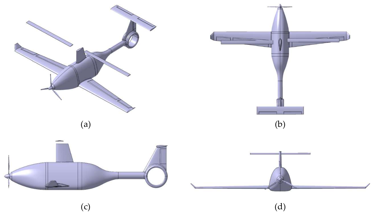
Figure 2.
High level schematics of VERTIGO HPS.
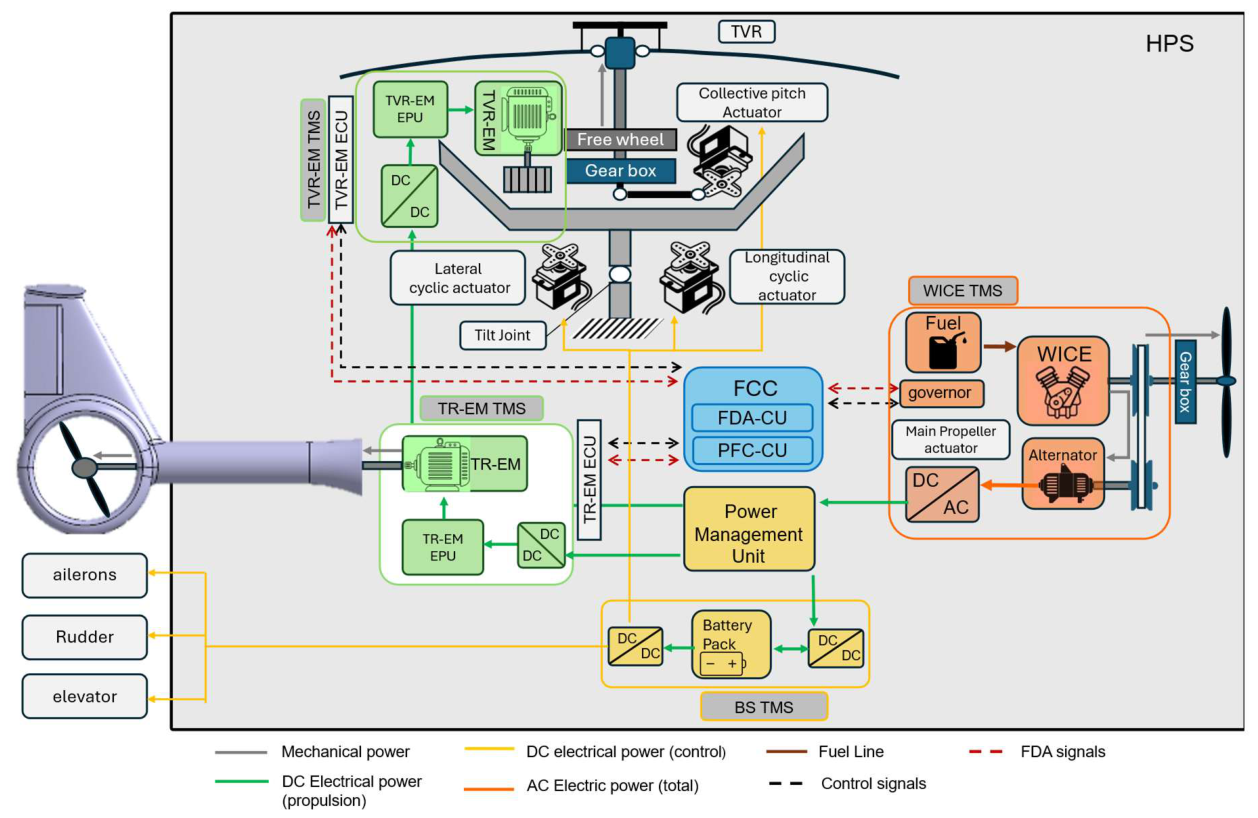
Figure 3.
Speed diagram of the generic blade section of the rotor.
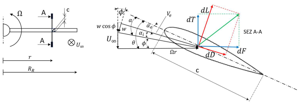
Figure 4.
Comparison between simplified and advanced BEMT implementation on NACA0006 profile: (a) induced angle of attack; (b) effective angle of attack; (c) thrust distribution per unit span; (d) in-plane force distribution per unit span.
Figure 4.
Comparison between simplified and advanced BEMT implementation on NACA0006 profile: (a) induced angle of attack; (b) effective angle of attack; (c) thrust distribution per unit span; (d) in-plane force distribution per unit span.
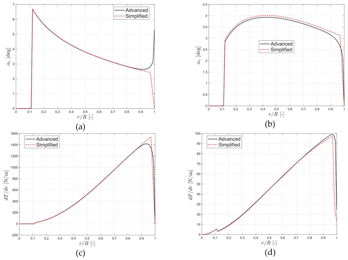
Figure 5.
. Main rotor aerodynamic coefficients in hover condition: (a) thrust; (b) torque.
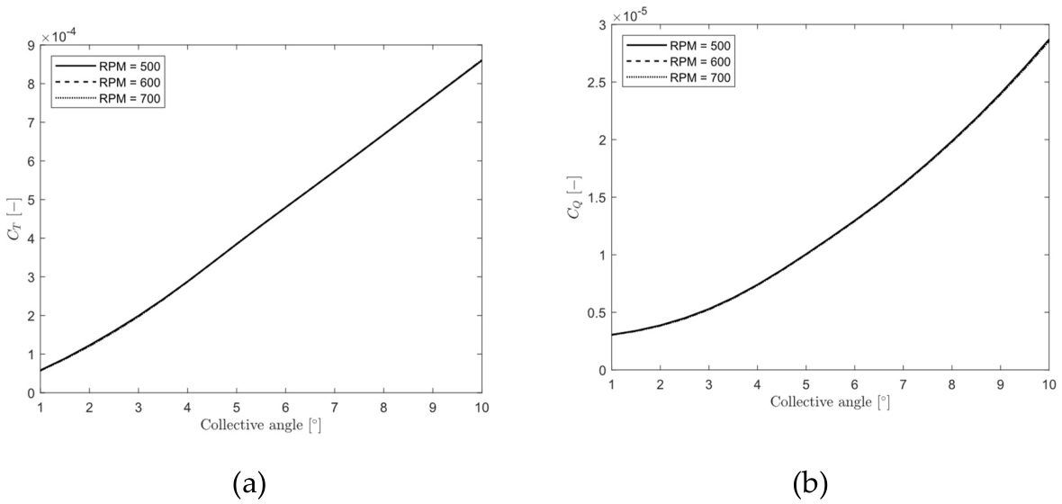
Figure 6.
. Main rotor aerodynamic coefficients in climb condition: (a) thrust; (b) torque.
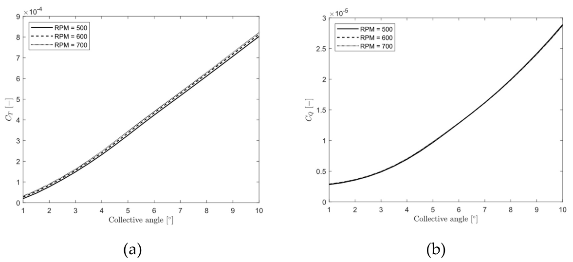
Figure 7.
Motor control architecture: current and speed loops with proportional-integral regulators.
Figure 7.
Motor control architecture: current and speed loops with proportional-integral regulators.
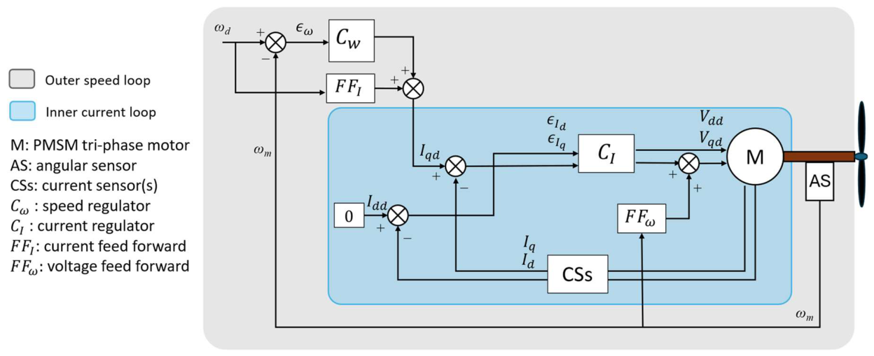
Figure 8.
High level scheme of the full nonlinear simulation model.
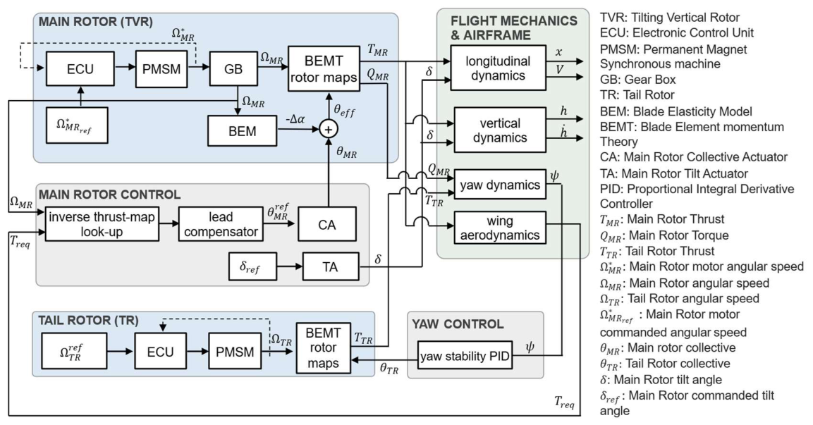
Figure 9.
Required power at the three vertical flight fixed-point conditions of hover, vertical climb and vertical descent for baseline and optimized operating values; (a) main rotor, (b) tail rotor.
Figure 9.
Required power at the three vertical flight fixed-point conditions of hover, vertical climb and vertical descent for baseline and optimized operating values; (a) main rotor, (b) tail rotor.
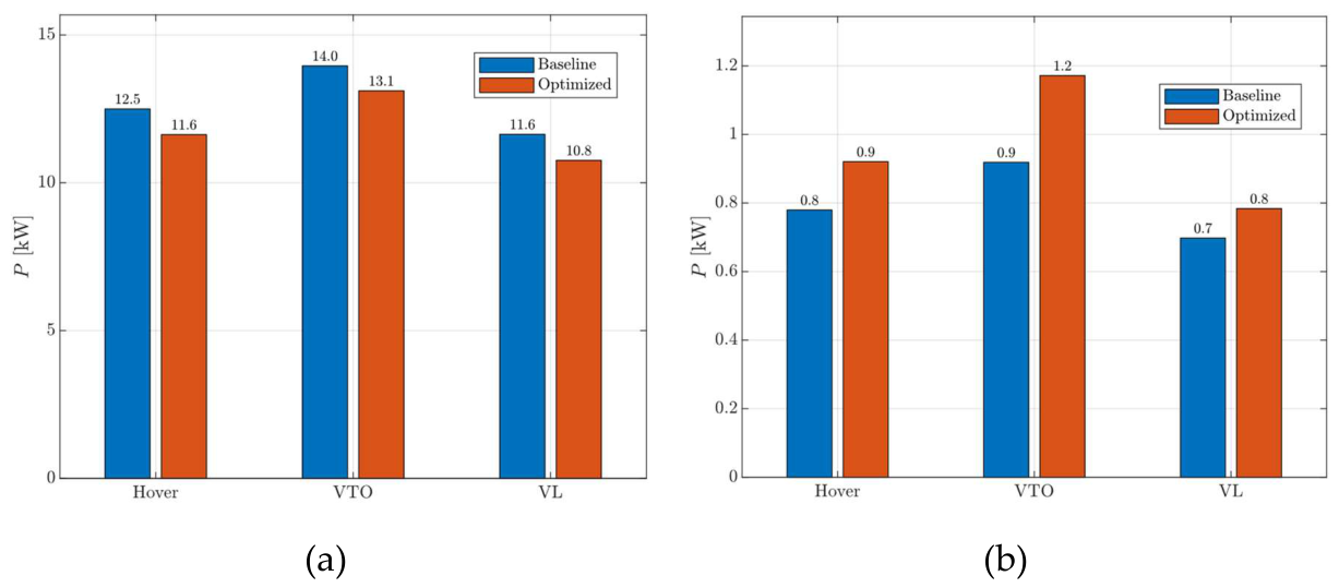
Figure 10.
Outcome of the fixed-point optimization expressed as relative changes with respect to the baseline operating point values, from left to right: main rotor speed, main rotor pitch angle, main rotor torque, main rotor absorbed power, total absorbed electrical power.
Figure 10.
Outcome of the fixed-point optimization expressed as relative changes with respect to the baseline operating point values, from left to right: main rotor speed, main rotor pitch angle, main rotor torque, main rotor absorbed power, total absorbed electrical power.
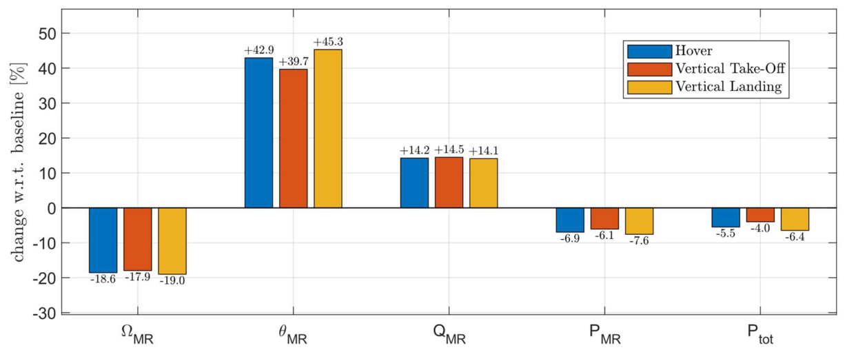
Figure 11.
Baseline transition on the nonlinear model; upper plot: main-rotor speed; mid plot: collective pitch; lower plot: flight speed. Dashed lines: upper actuation limits; dash-dot lines: lower limits derived from the rotor maps, namely the minimum speed that produces the required thrust at maximum collective and the minimum collective that produces it at maximum speed.
Figure 11.
Baseline transition on the nonlinear model; upper plot: main-rotor speed; mid plot: collective pitch; lower plot: flight speed. Dashed lines: upper actuation limits; dash-dot lines: lower limits derived from the rotor maps, namely the minimum speed that produces the required thrust at maximum collective and the minimum collective that produces it at maximum speed.
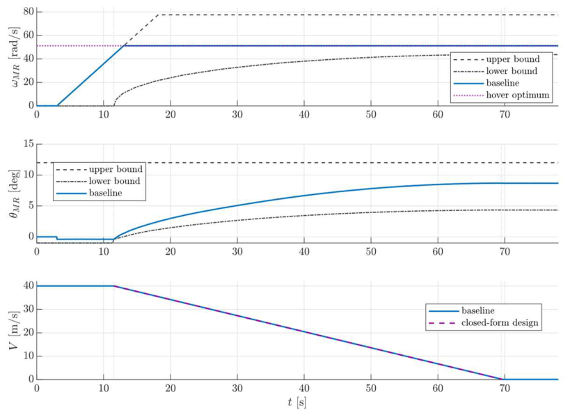
Figure 12.
Principal evaluation metrics of the baseline transition manoeuvre; (a) (upper plot) instantaneous electrical power of the main-rotor drive, of the tail-rotor drive and total; (lower plot) cumulative electrical energy; (b) (upper) wing lift, vertical rotor thrust and their sum; (lower left) rotor thrust normalised by the weight versus normalized flight speed; (lower right) altitude and vertical speed.
Figure 12.
Principal evaluation metrics of the baseline transition manoeuvre; (a) (upper plot) instantaneous electrical power of the main-rotor drive, of the tail-rotor drive and total; (lower plot) cumulative electrical energy; (b) (upper) wing lift, vertical rotor thrust and their sum; (lower left) rotor thrust normalised by the weight versus normalized flight speed; (lower right) altitude and vertical speed.
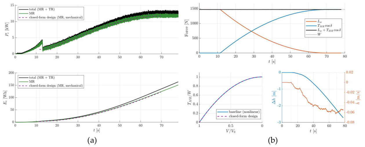
Figure 16.
Optimized transition on the nonlinear model, commands: (a) main-rotor speed; (b) main-rotor collective (commanded, delivered by the actuator, and effective at the blade after the elastic correction); (c) tail-rotor speed; (d) tail rotor collective.
Figure 16.
Optimized transition on the nonlinear model, commands: (a) main-rotor speed; (b) main-rotor collective (commanded, delivered by the actuator, and effective at the blade after the elastic correction); (c) tail-rotor speed; (d) tail rotor collective.
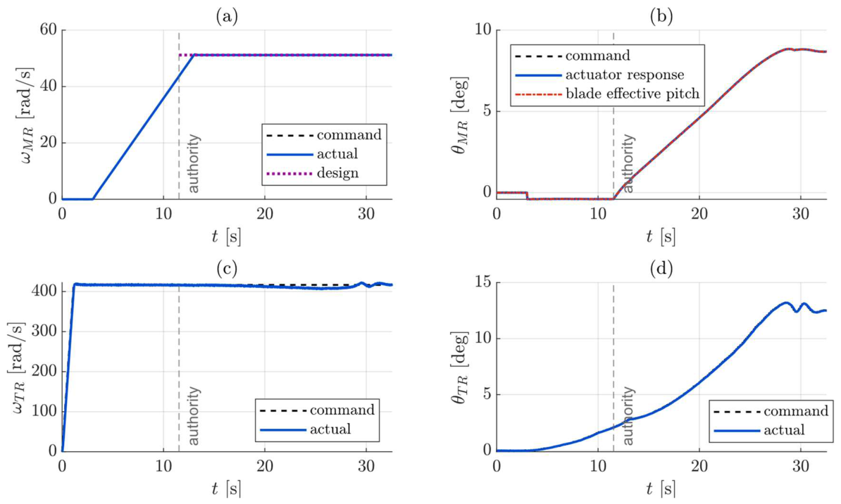
Figure 17.
Optimized transition on the nonlinear model, main rotor tilt angle (commanded, delivered, and closed-form design).
Figure 17.
Optimized transition on the nonlinear model, main rotor tilt angle (commanded, delivered, and closed-form design).
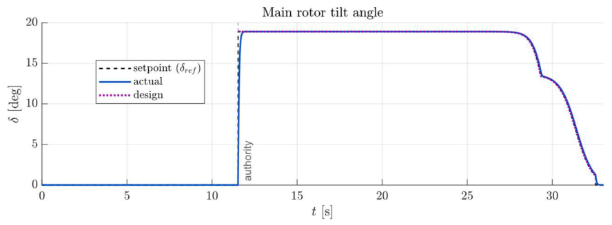
Figure 18.
Optimized transition on the nonlinear model, motion: (a) flight speed and distance against the closed-form design; (b) vertical speed and altitude excursion.
Figure 18.
Optimized transition on the nonlinear model, motion: (a) flight speed and distance against the closed-form design; (b) vertical speed and altitude excursion.
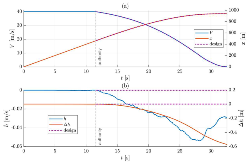
Figure 19.
Optimized transition on the nonlinear model, propulsion: (a) total and main-rotor electrical power against the closed-form main-rotor mechanical power; (b) cumulative electrical energy against the closed-form mechanical energy.
Figure 19.
Optimized transition on the nonlinear model, propulsion: (a) total and main-rotor electrical power against the closed-form main-rotor mechanical power; (b) cumulative electrical energy against the closed-form mechanical energy.
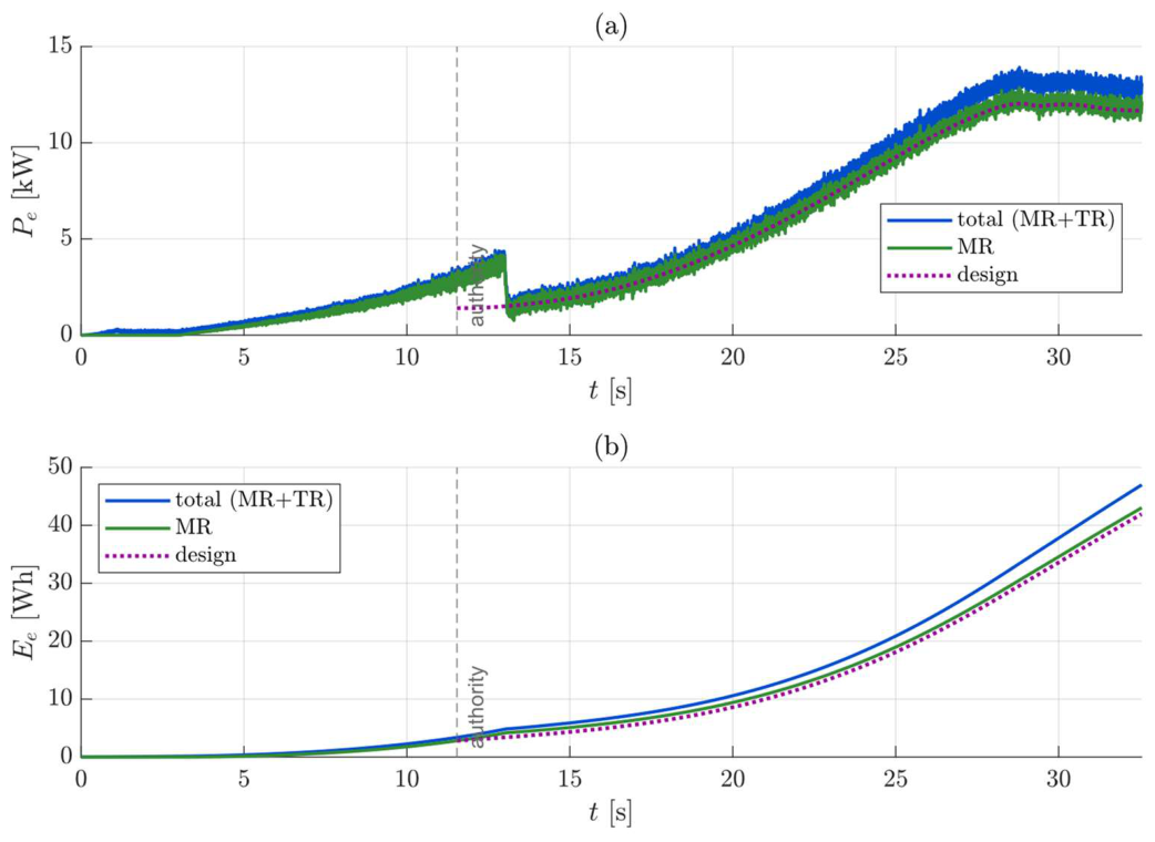
Figure 20.
Optimized transition on the nonlinear model, structure: (a) blade flapping angle; (b) flapping rate.
Figure 20.
Optimized transition on the nonlinear model, structure: (a) blade flapping angle; (b) flapping rate.
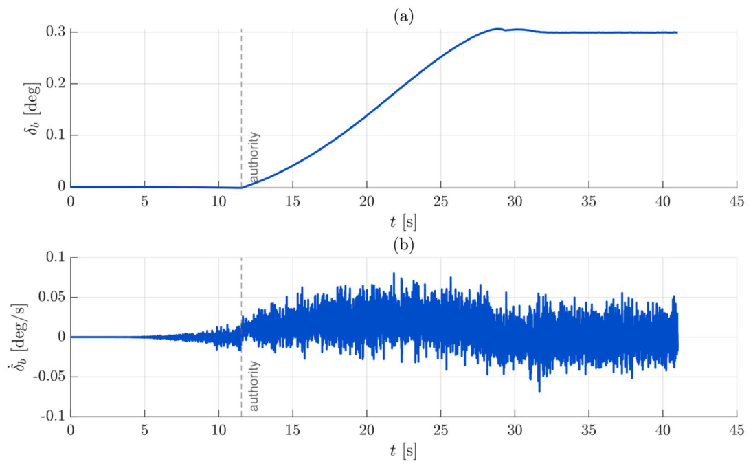
Figure 21.
Baseline and optimized transitions on the nonlinear model, on a common clock measured from the tilt engagement: (a) flight speed, with the closed-form designs dashed; (b) commanded tilt; (c) total electrical power; (d) cumulative electrical energy, annotated with the manoeuvre energy of each run at its own stop.
Figure 21.
Baseline and optimized transitions on the nonlinear model, on a common clock measured from the tilt engagement: (a) flight speed, with the closed-form designs dashed; (b) commanded tilt; (c) total electrical power; (d) cumulative electrical energy, annotated with the manoeuvre energy of each run at its own stop.
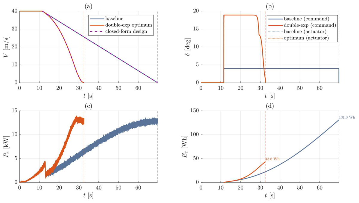
Figure 22.
Distributions of the output metrics over the uncertainty campaign, each normalized by its nominal value: histogram, kernel density estimate and Gaussian fit N(μ,σ), with the nominal value and the mean marked. (a) Peak electrical power; (b) maximum altitude excursion; (c) ground distance; (d) peak blade flapping rate.
Figure 22.
Distributions of the output metrics over the uncertainty campaign, each normalized by its nominal value: histogram, kernel density estimate and Gaussian fit N(μ,σ), with the nominal value and the mean marked. (a) Peak electrical power; (b) maximum altitude excursion; (c) ground distance; (d) peak blade flapping rate.
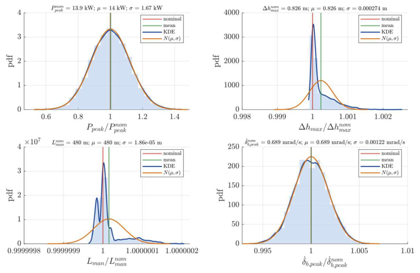
Figure 23.
First-order Sobol indices of the peak electrical power and of the peak blade flapping rate with respect to the three uncertain parameters, with the interaction share.
Figure 23.
First-order Sobol indices of the peak electrical power and of the peak blade flapping rate with respect to the three uncertain parameters, with the interaction share.
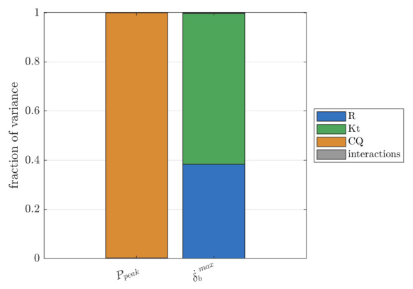
Figure 24.
Main effects: conditional mean of each output metric as a function of each uncertain parameter, with a ±2σ band. Abscissae: parameters normalized by their nominal values, the torque bias by the hover torque; ordinates: metrics normalized by their nominal values. The title of each row gives the nominal value of the metric.
Figure 24.
Main effects: conditional mean of each output metric as a function of each uncertain parameter, with a ±2σ band. Abscissae: parameters normalized by their nominal values, the torque bias by the hover torque; ordinates: metrics normalized by their nominal values. The title of each row gives the nominal value of the metric.
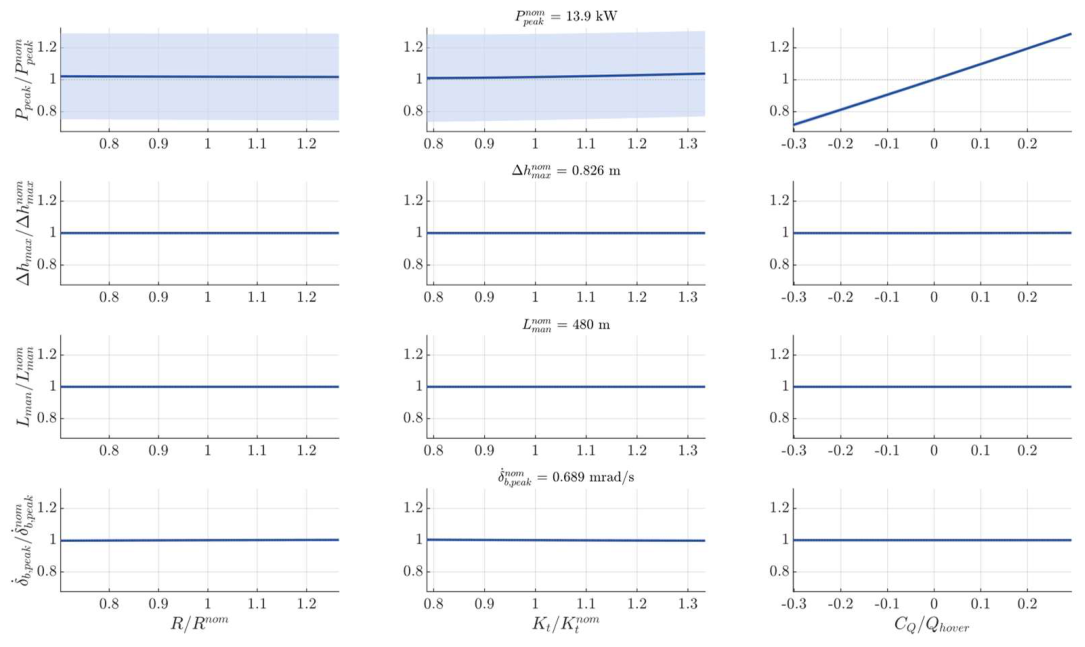

Table 1.
Main operational requirements of the VERTIGO copter-plane UAV.
| Characteristic | Value | Unit |
|---|---|---|
| Maximum take-off weight | 70–150 | kgf |
| Endurance in horizontal flight | 10 | h |
| Endurance in hover | 2 | h |
| Cruise speed | 40 | m/s |
| Maximum speed | 50 | m/s |
| Aerodynamic efficiency in horizontal flight | ≈10 | – |
| Maximum altitude in horizontal flight | 4500 | m |
| Maximum altitude in hover | 2500 | m |
| Operating temperature range | −15 to +49 | °C |
Table 2.
Definition of "prolonged stationary surveillance" mission.
| Phase | Altitude (m) | Duration (min) | Thrust control |
Lift control |
Attitude control |
|---|---|---|---|---|---|
| Vertical take-off | 0–200 | 2 | Rotors | Rotors | Rotors |
| Transition to forward flight* | 200 | 1 | Rotors/pusher | Rotors/wing | Rotors/a.s. |
| Climb* | 200–500 | 6 | Pusher | Wing | Aero surfaces |
| Cruise* | 500 | 11 | Pusher | Wing | Aero surfaces |
| Descent* | 500–200 | 3 | Pusher | Wing | Aero surfaces |
| Transition to hover* | 200 | 1 | Pusher/rotors | Rotors/wing | Rotors/a.s |
| Hover | 200 | 103 | Rotors | Rotors | Rotors |
| Vertical landing | 200–0 | 3 | Rotors | Rotors | Rotors |
* operated twice per mission.
Table 3.
Comparison between rotor performance predicted by simplified and advanced BEMT implementation in hover condition.
Table 3.
Comparison between rotor performance predicted by simplified and advanced BEMT implementation in hover condition.
| Parameter | Advanced BEMT | Simplified BEMT |
|---|---|---|
| Collective angle [deg] | 6.08 | 6.16 |
| Required thrust [N] | 1471.5 | 1471.5 |
| Torque [Nm] | 199 | 189.2 |
| Power [kW] | 12.5 | 11.9 |
| Convergence time (single simulation) [s] | 0.48 | 0.02 |
Table 4.
Bounds on the decision variables of the fixed-point optimization problem.
| Decision variable | Lower bound | Upper bound | Unit |
|---|---|---|---|
| Main rotor collective pitch | 3 | 15 | deg |
| Tail rotor collective pitch | −5 | 10 | deg |
| Main-rotor speed | 43.7 | 77.7 | rad/s |
| Tail rotor speed | 320 | 478 | rad/s |
Table 5.
. Parameters of the chosen permanent-magnet synchronous machines
| Parameter | Main rotor motor | Tail rotor motor | Unit |
|---|---|---|---|
| Model | 255-AAEI96-160 | 145-DZS96-012 | – |
| Rated Power | 13 | 1 | kW |
| Peak Power | 23 | 5.7 | kW |
| Rated speed | 3300 | 3000 | rpm |
| Rated torque | 36 | 3.6 | N m |
| Rated current | 160 | 12 | A rms |
| Maximum current | 600 | 60 | A rms |
| Pole pairs | 4 | 4 | – |
| Rotor inertia | 6.761 × 10⁻³ | 6.332 × 10⁻⁴ | kg m² |
| Viscous friction | 5 × 10⁻⁴ | 5 × 10⁻⁴ | N m s |
| Phase resistance | 1.0 | 10 | mΩ |
| Phase inductance | 5.31 | 53.1 | µH |
| Torque constant (datasheet) | 0.225 | 0.300 | N m / A rms |
| Torque constant (dq model) | 0.1299 | 0.1732 | N m / A |
| DC bus voltage | 96 | 96 | V |
| Machine efficiency | 0.93 | 0.93 | – |
| Converter efficiency | 0.96 | 0.96 | – |
| Transmission ratio | 600/3300 | direct drive | – |
Table 6.
Optima of the three tilt-law classes on the closed-form model, and the baseline evaluated on the same model. Energy and peak power refer to the main-rotor mechanical power at the fixed rotor speed of 51.2 rad/s; the cost J is normalized by the common population minima.
Table 6.
Optima of the three tilt-law classes on the closed-form model, and the baseline evaluated on the same model. Energy and peak power refer to the main-rotor mechanical power at the fixed rotor speed of 51.2 rad/s; the cost J is normalized by the common population minima.
| Tilt law | J* | E (Wh) | P_peak (kW) | t_stop (s) | l_stop (m) | δ at cruise (°) |
|---|---|---|---|---|---|---|
| A: free set-points, interpolated | 1.0613 | 39.6 | 12.00 | 21.3 | 484 | 14.9 |
| B: one-parameter shape | 1.0767 | 35.0 | 12.51 | 20.1 | 497 | 17.7 |
| C: double exponential | 1.0614 | 39.1 | 12.03 | 21.0 | 478 | 18.9 |
| Baseline, constant tilt | — | 119.1 | 11.71 | 58.2 | 1166 | 4.0 |
Table 7.
Baseline and optimized transitions compared on the nonlinear model and on the closed-form model. Energy and time are measured from the tilt engagement to the stop of each manoeuvre.
Table 7.
Baseline and optimized transitions compared on the nonlinear model and on the closed-form model. Energy and time are measured from the tilt engagement to the stop of each manoeuvre.
| Quantity | Baseline | Optimized | Change |
|---|---|---|---|
| Tilt at cruise speed [°] | 4.00 | 18.9 | — |
| Stop time from tilt engagement, nonlinear [s] | 58.17 | 21.01 | −63.9 % |
| Stop time from tilt engagement, closed form [s] | 58.16 | 21.01 | −63.9 % |
| Ground distance, nonlinear [m] | 1166 | 479 | −58.9 % |
| Ground distance, closed form [m] | 1166 | 478 | −59.0 % |
| Electrical energy, nonlinear [Wh] | 131.0 | 43.6 | −66.7 % |
| Main-rotor mechanical energy, closed form [Wh] | 119.1 | 39.1 | −67.1 % |
| Peak total electrical power, nonlinear [kW] | 13.53 | 13.93 | +3.0 % |
| Maximum altitude excursion, nonlinear [m] | 2.25 | 0.57 | −75 % |
Table 8.
Uncertainty campaign on the optimized manoeuvre, 216,000-run factorial grid: nominal value, mean, coefficient of variation, 5th–95th percentile range and first-order Sobol indices with respect to the phase resistance R, the torque constant Kt and the torque bias CQ of the main drivetrain. The Sobol indices of the altitude excursion and of the ground distance decompose a variance at the level of the integrator round-off and carry no physical meaning.
Table 8.
Uncertainty campaign on the optimized manoeuvre, 216,000-run factorial grid: nominal value, mean, coefficient of variation, 5th–95th percentile range and first-order Sobol indices with respect to the phase resistance R, the torque constant Kt and the torque bias CQ of the main drivetrain. The Sobol indices of the altitude excursion and of the ground distance decompose a variance at the level of the integrator round-off and carry no physical meaning.
| Metric | Nominal | Mean | CoV | P5 – P95 | S_R | S_Kt | S_CQ |
|---|---|---|---|---|---|---|---|
| Peak total electrical power [kW] | 13.93 | 14.19 | 13.3 % | 10.85 – 17.45 | < 0.001 | 0.002 | 0.998 |
| Maximum altitude excursion [m] | 0.826 | 0.826 | 0.04 % | 0.8256 – 0.8265 | < 0.001 | 0.001 | 0.985 |
| Ground distance [m] | 479.83 | 479.83 | < 0.001 % | 479.83 – 479.83 | 0.003 | 0.100 | 0.887 |
| Peak blade flapping rate [mrad/s] | 0.689 | 0.689 | 0.17 % | 0.687 – 0.691 | 0.384 | 0.613 | < 0.001 |
Disclaimer/Publisher’s Note: The statements, opinions and data contained in all publications are solely those of the individual author(s) and contributor(s) and not of MDPI and/or the editor(s). MDPI and/or the editor(s) disclaim responsibility for any injury to people or property resulting from any ideas, methods, instructions or products referred to in the content. |
© 2026 by the authors. Licensee MDPI, Basel, Switzerland. This article is an open access article distributed under the terms and conditions of the Creative Commons Attribution (CC BY) license (http://creativecommons.org/licenses/by/4.0/).
Copyright: This open access article is published under a Creative Commons CC BY 4.0 license, which permit the free download, distribution, and reuse, provided that the author and preprint are cited in any reuse.