

Submitted:
19 October 2026
Posted:
20 October 2026
You are already at the latest version
Abstract
Spontaneous subatomic mass–energy interconversion has been proposed as a microscopic stochastic process connecting quantum coherence with effective gravitational dynamics. I reconstruct the hypothesis as restricted mathematical models and confront it with published interferometric and cosmological measurements rather than presuming its empirical success. Gaussian differential mass noise yields a correlation-dependent attenuation of two-path fringe visibility; perfectly common-mode noise cancels. Published molecular interferometry extending beyond 25,000 Da reports selected fringe visibilities exceeding 90% of the quantum-theory expectation. Under explicit simplifying assumptions this corresponds to an illustrative residual phase-variance budget below 0.211 rad², not a calibrated confidence limit on microscopic noise. Cosmological benchmarks comprise Planck and ACT cosmic-microwave-background constraints, the SH0ES distance ladder, Pantheon+ supernovae, and DESI DR2 baryon acoustic oscillations. I calculate fixed-Planck ΛCDM distances for 13 DESI DR2 measurements and report descriptive residuals, carefully distinguishing these standard-model calculations from unavailable interconversion-specific predictions. Covariant stress-energy accounting, Bell locality, noise positivity, radiative stability, and singularity conditions remain mandatory consistency requirements. Neither quantum interference nor the Hubble discrepancy independently demonstrates interconversion. The resulting synthesis identifies observational restrictions, the missing links between microscopic noise and cosmological dynamics, and the specifications needed for a future parameter-estimating SMEI test.
Keywords:
stochastic mass–energy interconversion
; foundations of quantum mechanics
; matter-wave interferometry
; Einstein–Langevin equation
; emergent gravity
; falsifiability
1. Introduction: The Physical Question and the Scope of the Proposal
Quantum theory and general relativity have exceptionally successful empirical domains, but their conventional formulations use different notions of state, dynamics, and the physical role of spacetime. A satisfactory quantum theory of gravity remains open. This fact does not imply that the Schrödinger equation and Einstein equations are mutually inconsistent wherever each is applicable; rather, it signals unresolved questions about quantum sources, backreaction, spacetime microstructure, and the appropriate limiting procedures. Gravitational singularities and the cosmological-constant problem make these questions particularly acute [12,13,14,15,16,23,24].
A family of papers by Willis has proposed spontaneous subatomic mass–energy interconversion (SMEI) as a possible physical substrate for quantum uncertainty, wave–particle duality, and the emergence of smooth gravitational geometry [1,2,3]. The earliest article presented a fluctuating-mass hypothesis with broad implications for quantum mechanics [1]. A subsequent treatment explored kinetic-phase fluctuations and interferometric visibility [2]. The recent bridge formulation represented localized interconversion events statistically, distinguishing their ensemble-mean stress-energy contribution from a residual covariance capable of sourcing gravitational fluctuations [3]. These articles motivate the present synthesis; their proposed physical mechanisms are not treated here as experimentally demonstrated facts.
A philosophical discussion would be relevant to Karl Popper’s critical rationalism, objective propensities, scientific realism, cosmological time, and emergent gravitation [4,5,6,28]. Those issues remain relevant. However, philosophical desirability cannot stand in place of dynamical specification. This work asks a narrower and more scientifically decisive question: what can be derived from clearly stated stochastic assumptions, what remains unproved, and what observations would distinguish SMEI from ordinary quantum dynamics, environmental decoherence, and general-relativistic cosmology?
The paper makes four contributions. First, it presents a minimal mass-noise model and derives an illustrative phase-noise visibility law, explicitly retaining cross-path correlations. Second, it presents a covariant event-process language in which an average stress tensor and a connected noise kernel arise from one probability law, with conservation and positivity imposed rather than assumed. Third, it confronts major no-go and consistency constraints, including the Bell–CHSH inequality, gauge and Lorentz symmetry, energy bookkeeping, radiative stability, and the conditions governing cosmological bounces. Fourth, it states falsification and parameter-identifiability criteria suitable for pre-registered experimental and observational analyses. Published interferometric and cosmological summary measurements are now confronted with the conditional formulas and a reproducible fixed-parameter baseline, but no event-level interferometric data fit, SMEI cosmological likelihood analysis, or microscopic field-theoretic derivation is claimed.
The proposed relationship with other approaches must be stated accurately. Nelson’s stochastic mechanics already connected a diffusion coefficient D = ℏ/(2m) with a route to Schrödinger dynamics [7]. Environment-induced decoherence [8] and dynamical-collapse theories [9] already provide physically different stochastic descriptions and test programs. Jacobson’s thermodynamic derivation of Einstein’s equations [12], stochastic gravity [13], and entropic-gravity proposals [14] likewise establish substantial preceding literature. The distinctive SMEI question is whether a specified mass–energy conversion mechanism, rather than merely an unspecified stochastic influence, can furnish simultaneously consistent microphysical and gravitational source terms.
2. Historical and Epistemological Foundations
2.1. From Geometric Determinism to Objective Probabilities
General relativity describes gravitational phenomena in terms of spacetime geometry and matter stress-energy, while textbook quantum mechanics assigns probabilistic measurement outcomes to Hilbert-space states. These distinct structures do not license the claims that relativity is simply a rigid clockwork or that all formulations of quantum mechanics require a conscious observer. Quantum decoherence explains important aspects of effective classicality without observer-induced collapse, although it does not by itself uniquely settle every interpretation of measurement [8,27]. Interpretations differ in ontology, not in the experimentally confirmed core predictions of standard quantum theory.
Popper proposed objective propensities as probabilities associated with physical situations, rather than merely expressions of subjective ignorance [5]. SMEI can be read as a candidate physical realization of propensity: its random-event law assigns reproducible conditional distributions to outcomes for a specified preparation and experimental geometry. But the interpretation is useful only when those distributions are connected to observables. An invariant measure, noise spectrum, and a calibration rule provide more physical content than describing particles metaphorically as jittering or matter as a thermodynamic fluid.
The distinction between an ontological picture and a successful dynamical theory is indispensable. Postulating real fluctuating events is compatible with realism; it does not demonstrate that the hypothesized events exist. Popperian falsifiability concerns the logical exposure of specific theoretical statements to possible evidence [4]. A model whose event amplitude can always be adjusted continuously toward zero may remain compatible with all observations while providing no distinctive corroboration. For this reason, the present treatment separates parameter estimation from discriminating predictions and explicitly identifies the model’s null limits.
2.2. Scientific Alternatives are Not Interchangeable
The philosophical case should not rely on caricatures of competing research programs. String theory has mathematically developed sectors and indirect research motivations, while loop quantum gravity investigates background-independent quantization; neither may be dismissed solely because direct Planck-scale tests are challenging. Dawid has analyzed non-empirical theory assessment, not demonstrated that competing frameworks are scientifically meaningless [22]. Similarly, renormalization in quantum field theory is not simply an arbitrary subtraction of impossible infinities. A stochastic replacement needs a regulator, a consistent stress tensor, a renormalization prescription when quantum fields are involved, and measurable predictions of its own [13,23].
SMEI is therefore currently proposed here as a phenomenological extension and research program, not a verified theory of everything, nor a replacement for quantum field theory, and not yet a proof of the emergence of spacetime. Its viability depends on reproducing established tests at least as accurately as existing theories and surviving new cross-domain constraints.
3. Minimal Microscopic Mass-Noise Model
3.1. Definition and perturbative Hamiltonian
For a nonrelativistic particle of reference inertial mass m0 > 0, introduce a dimensionless stochastic process η(t) and write
m(t) = m0[1 + η(t)], ⟨η(t)⟩ = 0, |η(t)| ≪ 1.
The brackets denote an ensemble average over runs or realizations. Positivity demands 1 + η(t) > 0 for every physically admitted realization; a strictly Gaussian process with unbounded tails is consequently only a controlled small-noise approximation, not a complete microscopic mass distribution. Its covariance is
Cη(t,t') = ⟨η(t)η(t')⟩, Cη ≽ 0.
Here positive semidefiniteness means for every real test function f. The energy difference ΔE = c2Δm is a mass–energy accounting relation. It is not by itself a dynamical law for force, momentum transfer, spontaneous emission, or particle localization. A consistent microscopic account must specify what degree of freedom gains the compensating energy, or else provide a fully coupled open-system model in which the subsystem mass is stochastic while the total conserved energy remains well defined.
For a spatially uniform time-dependent inertial mass, an illustrative laboratory-frame Hamiltonian is
The expansion holds under the stated weak-noise assumption; H0 = K0 + V. If mass also depends on position, naive multiplication p2/[2m(x,t)] is not generally a self-adjoint kinetic operator. A symmetric choice is , supplemented as necessary by a field-theoretic derivation. Moreover, the nonrelativistic Hamiltonian is a controlled approximation, not evidence that a fundamental elementary-particle rest mass literally changes. In relativistic quantum field theory such a claim requires Lorentz-covariant, gauge-consistent new interactions and stringent constraints from spectroscopy and precision measurements.
One may formalize subsystem exchange with an interaction current Jν:
The labels p and env refer to the effective particle and compensating environment sectors, not necessarily to a literal material fluid. Equation (4) is a consistency requirement; the present article does not derive the microscopic current. Any complete SMEI model must do so, while avoiding double counting rest energy and fluctuation energy.
3.2. Relation to Diffusion and the Uncertainty Principle
In Nelson’s model the diffusion coefficient is D = ℏ/(2m0) [7]. The earlier SMEI discussion used this characteristic scale to motivate an objective stochastic interpretation [1]. A coefficient of this numerical form, however, cannot be inferred from Eq. (1) without an independent Langevin or stochastic-action law and its noise–dissipation structure. An arbitrary mass process need not generate Brownian translation, and a stochastic trajectory need not reproduce the complex Schrödinger amplitude, phase, or Born rule.
The Robertson uncertainty inequality follows from operator noncommutativity,
Equation (5) is established within quantum mechanics; SMEI has not independently derived it from Eqs. (1)–(4). The appropriate program is to show how a proposed stochastic evolution recovers the quantum commutator, the Born probability rule, and unitary evolution in the noise-free regime, before interpreting the quantum uncertainty relation as a consequence of mass exchange. This statement preserves the motivating hypothesis while avoiding circular reasoning.
4. Interference, Phases, and a Testable Visibility Law
4.1. What Fluctuates in an Interferometer?
A single detection event appears localized, while repeated events exhibit a two-path interference distribution. Standard quantum mechanics accounts quantitatively for both. SMEI adds a proposed kinetic-phase channel in which an effective mass fluctuation modifies phase accumulation [2]. For paths j = 1,2, assume a controlled semiclassical kinetic-energy history Kj(t) and weak path-sampled noise ηj(t). To first order in η, the additional phase difference can be written
The overall phase sign is immaterial for the visibility; Eq. (6) follows from the −ηK0 perturbation and the usual action-phase convention. Its path dependence is fundamental. If the two arms have identical kinetic weighting and experience the same noise realization, the added phase is common mode and cancels: Δϕ = 0. Therefore zero-mean mass fluctuation alone does not predict observable decoherence. Any universal statement that coherence necessarily falls with increasing particle mass or flight time is too strong without specifying correlations, trajectories, and apparatus couplings.
Write Δη(t) = η1(t) − η2(t) for paths of equal approximate kinetic energy K. Then
The experiment measures the modulus of an averaged phase factor. With all ordinary decoherence channels either independently calibrated or kept in the baseline visibility 0,
For stationary zero-mean Gaussian differential noise, the cumulant theorem gives the conditional result
Equation (9), rather than a generic claim of interference smearing, supplies an operationally measurable object. It presupposes Gaussian noise, negligible backreaction on the paths, a known trajectory, and a valid separation of the proposed channel from electromagnetic, mechanical, thermal, collisional, and readout noise.
4.2. Illustrative Correlated-Noise Example
For a single-parameter illustration take with correlation time τc > 0. Double integration yields
The short-duration and long-duration limits are respectively
These are illustrative results conditional on the chosen covariance, not predictions that experiments have confirmed or numerical bounds inferred from published datasets. At fixed speed v, K = m0v2/2 and the exponent scales as if σΔ and τc are species-independent. At fixed momentum p, K = p2/(2m0) and the scaling is instead . A mass-dependent noise spectrum could change either result. A test of SMEI must specify which variables are controlled and why the noise parameters should or should not vary by species.
The spectrum SΔ(ω) defined by the Fourier transform of CΔ(τ) offers a further form:
The filter function in Eq. (12) makes measurement timing and noise color explicit. In an unbalanced apparatus the two kinetic-energy weighting functions replace the common K; correlated acceleration or phase noise could mimic the effect. Data fitting must include these nuisance parameters and specify the assumed spatial correlation length of the putative SMEI process.
4.3. Phase Diffusion is Not Automatically Collapse
Phase averaging can reduce off-diagonal coherence in an ensemble while leaving every individual realization governed by a unitary Schrödinger equation. It does not, by itself, explain why a unique detector event occurs or derive a new collapse postulate. Objective-collapse frameworks introduce nonunitary stochastic dynamics with accompanying constraints such as heating or spontaneous radiation [9]. The present perturbative mass-noise model does not claim those effects until its dynamical law and detector coupling are constructed. Nor should the vivid picture of a localized particle guided by pressure waves through both slits be treated as a deduction: such waves would require an explicit relativistic field equation, boundary conditions at both slits, and a derivation of the observed fringes.
Modern interferometry already supplies powerful tests of modifications to quantum mechanics [20,21]. In particular, coherent superpositions of large molecules establish that interference survives in increasingly massive systems [21]. A putative SMEI visibility term must be small enough to respect the published visibility and experimental uncertainties, and it must be assessed against ordinary environmental decoherence [8,20]. Section 4.4 now gives a transparent numerical attenuation budget for a selected published high-visibility result, but it remains unjustified to infer a statistical limit on σΔ or τc without the experiment-specific likelihood and flight geometry.
4.4. Confrontation With Published Interferometry Rather Than Generic Visibility Claims
The test proposed in Sec. 4 can be anchored to actual matter-wave interference observations. This section reports published experimental results, distinguishes them from conditional SMEI calculations, and avoids treating agreement with quantum mechanics as proof of mass interconversion. Table 1 covers complementary molecular and atomic regimes. Gerlich et al. demonstrated near-field interference of organic molecules as large as 6,910 u and 430 atoms, with calculated ordinary environmental decoherence estimated to be small in the selected operating regime [29]. Eibenberger et al. subsequently reported interference for molecules exceeding 10,000 u and containing 810 atoms [30]. Kovachy et al. observed atom-wavepacket interference after a spatial separation of approximately 54 cm, probing a different scale from macromolecular mass [31]. Fein et al. reported fringes for molecules exceeding 25,000 Da, up to 2,000 atoms, with the observed interference visibility in the reported high-visibility cases exceeding 90% of the quantum expectation [21]. None of these studies measured spontaneous SMEI events directly.
For a transparent illustrative comparison, use the reported high-visibility molecular benchmark R > 0.90 and assume, solely for this calculation, that every attenuation remaining after the quoted quantum-theory baseline were caused by nonnegative Gaussian SMEI differential dephasing. Equations (8)–(9) imply R = exp(−χSMEI) and hence
χSMEI = −lnR < −ln(0.90) = 0.10536, Var(δϕ) = 2χSMEI < 0.21072 rad2.
This is not a statistically calibrated upper limit. The source’s phrase “more than 90% of the expected visibility” does not provide a full likelihood, calibrated error distribution, or the raw visibilities for every configuration. The estimate applies only to the specified high-contrast configuration and its assumed normalization; ordinary visibility-reduction channels and baseline-model uncertainty must be marginalized. A correct likelihood would fit obs with published systematic and statistical uncertainties and theoretical QM derived from the complete grating response, including all environmental loss. Without flight-time, velocity distribution, actual arm trajectories, and CΔ at the corresponding path separation, Eq. (13) cannot be converted into an empirical value of σΔ, τc, or an interconversion-event rate. The 2011 environmental-decoherence estimate of less than approximately 1% in some operating conditions [29] is likewise a physical model estimate, not an observed SMEI residual.
Equation (28) already excludes, conditional on all its assumptions, a phenomenological SMEI variant predicting χSMEI≳0.105 in that same experimental setting. It does not exclude a common-mode process (CΔ = 0), a model that predicts much weaker noise, or a mechanism that leaves standard interference untouched. The independent 54-cm atomic superposition [31] is valuable precisely because a future spatial covariance function could turn its different path separation into a joint parameter test. A credible unified mass-noise model would fit at least two such experiments with the same coupling law, a specified species dependence, and geometry-dependent cross-path correlations.
4.5. Practical Path From Published Plots to a True Interferometric Likelihood
A quantitative reanalysis would obtain the visibility-versus-laser-power points and covariance from the molecular studies [21,29,30], or raw phase records for an atomic instrument [31]. For each experimental configuration j, construct χj(θ) from Eq. (12), with θ a common physically derived parameter vector. Write , where ν describes independently constrained nuisance terms such as vibrations, residual-gas scattering, blackbody interactions, molecular velocity distribution, laser power, alignment, and detector response. Publish the observation covariance and controls, then compare the SMEI-augmented likelihood with the χ = 0 null hypothesis. The present article does not claim to have obtained those event-level experimental files or fitted such a likelihood.
5. Entanglement, Bell inequalities, and Locality
The original philosophical proposal sought to interpret spatially separated entanglement correlations as products of a common stochastic history and a shared background field. Such intuitions are not sufficient to reproduce Bell-violating correlations. For a conventional local hidden-variable model with measurement settings a,b and hidden variable λ, outcomes factorize as
P(A,B∣a,b,λ) = P(A∣a,λ)P(B∣b,λ), ρ(λ∣a,b) = ρ(λ).
Under this locality factorization together with measurement independence and the relevant outcome assumptions, the Clauser–Horne–Shimony–Holt (CHSH) combination satisfies
S = |E(a,b) + E(a,b') + E(a',b) − E(a',b')| ≤ 2.
Quantum theory permits for suitable entangled states and settings. The framework of Bell’s theorem [10] and later CHSH tests [26] is supported by loophole-reducing experiments including Hensen and colleagues [11]. Simply asserting that two particles share synchronized classical noise or that the same local field is present at both stations leaves Eq. (15) in force when the assumptions of Eq. (14) hold. Correlation is not the same as reproducing the full conditional quantum distribution.
Consequently SMEI faces a genuine fork. One route is to treat its micro-events as an ontic stochastic supplement to quantum theory while retaining the quantum nonseparability required to reproduce Bell correlations; then it is not a completely local hidden-variable replacement. Another route is to specify exactly which assumption underlying Eq. (15) is not satisfied, while proving compatibility with no-signalling and the complete experimental statistics. A third possibility is to restrict the stochastic hypothesis to interferometric phase noise and gravitational coarse-graining, leaving the interpretation of Bell entanglement open. This paper adopts the third, conservative position. It does not claim that SMEI has explained loophole-free Bell violations.
That restraint also corrects the earlier characterization of Bohmian or pilot-wave approaches. A real particle trajectory can coexist with successful quantum predictions, but the orthodox Bohmian construction is generally nonlocal for entangled multi-particle systems [25]. Realism and strict Bell locality must not be conflated.
6. Covariant Event-Process Representation of the Gravitational Sector
6.1. A marked Random Measure
The bridge formulation [3] suggests modeling localized exchange events by a covariant marked point process. Let za denote spacetime event locations and αa marks encoding exchanged energy, duration, tensor structure, and internal reservoir labels. Schematically define
The event kernels qμν must be smooth or distributionally meaningful and must transform tensorially. A coordinate-independent intensity measure can be written , with ν a scalar event intensity per proper four-volume, assuming units and normalization of marks are specified consistently. The use of does not alone prove a complete diffeomorphism-invariant microphysical theory; invariance must hold also for kernels, mark distributions, and the action.
For a marked Poisson ansatz the characteristic functional of a linear probe Jμν takes the form
Equation (16) is a convenient formal assumption, not an experimentally established distribution of spacetime events. Functional derivatives generate connected statistical moments. For example, with the obvious shorthand for event averages,
These formulas require independent Poisson events. Correlated or clustered exchange processes add higher connected correlations and can change the scaling. Crucially, positivity is automatic for a genuine classical covariance: for real test tensors f. Not every arbitrarily proposed covariance has this property.
6.2. Conservation and the Einstein–Langevin Limit
The averaged total stress tensor entering Einstein’s field equations must satisfy the contracted Bianchi identity. Separating mean and fluctuations,
If exchange between event and reservoir sectors is present, the separate tensors need not be conserved; their sum must be. If every realized total source is divergence-free, its fluctuations are transverse in the appropriate distributional sense. Choosing an arbitrary N and an unrelated exchange rule will not generally satisfy that constraint. The background equations may be written
Linearizing gives, in schematic gauge-fixed form,
This form is motivated by the established Einstein–Langevin framework of stochastic semiclassical gravity [13]. It is important not to equate its quantum stress-tensor noise kernel automatically with the classical Poisson-event kernel in Eq. (19). Equivalence or a justified approximation between those objects would require a microscopic derivation. Nor does Eq. (22) quantize gravitational degrees of freedom. It is a phenomenological equation for stochastic metric response to source fluctuations.
6.3. Coarse-Graining and What It Does Not Establish
For independent events with finite variance, a region containing an expected event count has relative mean-source fluctuations suppressed roughly as . More generally, standardized cumulants of order n > 2 scale as if the relevant independent-event assumptions hold. Long-range correlations, heavy tails, or nonstationarity can invalidate Gaussian coarse-graining. This supplies a mathematical route to smoothness of an effective source, not an ontological deduction that spacetime itself is an illusion. The background metric remains part of the present event-process definition, so the construction cannot yet claim to derive all geometry from a spacetime-free substrate.
To obtain genuine emergent geometry, a deeper theory must define the event law without presupposing the very metric it is supposed to produce, or explicitly provide a renormalization-group or self-consistency fixed point leading from pregeometric variables to metric distance and causal order. The present formulation represents a possible bridge within a geometric framework. It is therefore compatible with studying emergence without having completed its derivation.
7. Lorentz Invariance, Field Theory, and Radiative Stability
A universal noise process η(t) defined relative to one laboratory time selects a preferred foliation. Such an ansatz is acceptable for a limited nonrelativistic phenomenological experiment but cannot serve unmodified as a Lorentz-invariant fundamental law. A relativistic completion might introduce a scalar field χ(x) coupled to an effective mass, meff(x) = m0 + gχ(x), or a covariant stochastic influence functional. Both choices introduce new dynamics and possible fifth-force, equivalence-principle, and spectral constraints. The scalar coupling must be justified for each particle species and made compatible with Standard Model gauge structure.
A toy relativistic matter action would take the form
with the usual qualifications about units, spin connection, and quantum renormalization. Equation (22) is displayed solely as an example of what a covariant completion would have to specify, not a derived SMEI field equation. Field fluctuations generally carry stress-energy and produce radiative corrections to masses and couplings. A credible completion should assess whether the assumed stochastic term respects gauge identities and unitarity, whether its spectrum causes unacceptable heating, diffusion, or emission, and whether counterterms are stable under quantum corrections.
An analogous issue appears in conservation. A particle’s changing rest mass can be represented as exchange with another field, but if that field is omitted the model may violate local stress-energy conservation. Because the gravitational field couples to total stress-energy, the compensating sector cannot be treated as an invisible bookkeeping device in cosmology. It influences background evolution and perturbations. These requirements are not technical embellishments: failure of conservation or positivity would disqualify the construction before philosophical conclusions are considered.
8. Cosmology, Dark Energy, and the Hubble-Constant Problem
8.1. From Event Rates to an Effective Density
The bridge article [3] offers a useful dimensional dictionary. If events occur with proper rate r per unit physical volume per unit proper time, each carrying an energy E for an effective lifetime τ, a stationary shot-noise estimate is
Equation (23) is an energy-density estimate, not an equation of state and not a solution to the cosmological-constant problem. The sign, pressure, perturbations, and dependence on temperature and curvature require a stress-tensor calculation. A spatially homogeneous and isotropic population of events can yield a perfect fluid with energy density ρ and pressure p, but homogeneity and isotropy alone do not force p = −ρ. A fully Lorentz-invariant vacuum-like expectation value has the stronger form in the usual metric convention. For an evolving component define w = p/ρ and use total conservation to obtain
Here energy density and pressure use consistent c = 1 cosmological units in Eqs. (25)–(32), and Q represents exchange with other cosmic sectors. The zero-mean condition ⟨ΔT⟩=0 for residual noise does not generate a positive vacuum density; any contribution must come from a nonzero mean, correlations through a derived effective action, or a specified backreaction term. A finite event rate also does not guarantee that the renormalized vacuum energy has the observed tiny magnitude [23].
8.2. A possible Early-Time Transient—Not a Demonstrated Resolution
The Hubble tension compares early-universe inferences under a cosmological model with direct late-universe distance-ladder determinations, among other measurements [17,18]. Early dark energy (EDE) has been explored as a mechanism that can alter the pre-recombination sound horizon [19]. In an SMEI-inspired scenario an event population might contribute a short-lived energy component near that epoch, but this possibility does not establish that the model resolves the tension. The expansion history would obey
The parameters in r(z), ⟨Eτ⟩, w(a), and Q(a) must be set before predictions for the cosmic microwave background are computed. A higher early energy density tends to increase H(z) and can reduce rs, but the inference of H0 depends on the full fit to peak structure, damping, lensing, baryon acoustic oscillations, supernovae, nucleosynthesis, and growth of structure. Any successful cosmological implementation must run a Boltzmann perturbation solver and likelihood analysis and confront observational exclusions as well as appealing parameter shifts. Current cosmological data do not by themselves establish an SMEI contribution.
The early-universe noise sector would have its own density, velocity, and anisotropic-stress perturbations. These are not free to be tuned independently of the same event law that determines the background. The strongest distinctive test would be a shared-parameter restriction: the event statistics controlling the cosmological energy density and its perturbations should be linked by an explicit microscopic model to a nonzero part of the interferometric noise spectrum. If the sectors are given unrelated adjustable parameters, a claimed bridge remains primarily a juxtaposition of hypotheses.
8.3. Actual Cosmological Data: Planck, ACT DR6, SH0ES, and Pantheon+
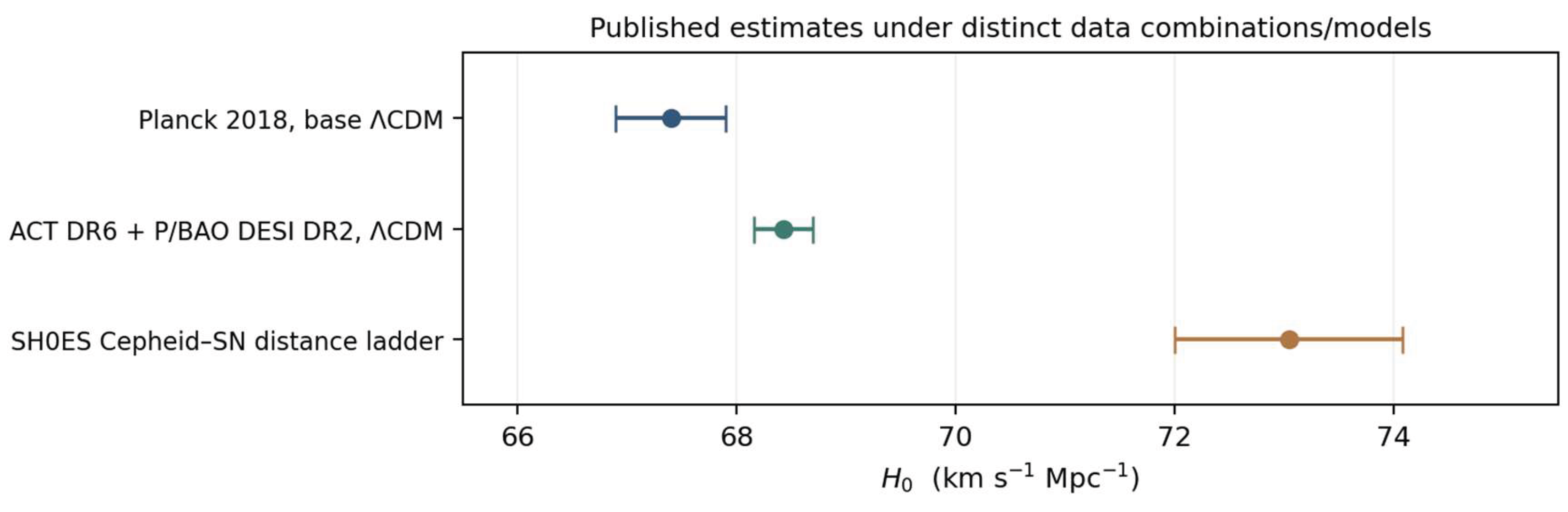
The magnitude of the cosmological challenge can be stated with published numbers rather than by attributing an unexplained expansion discrepancy to stochastic conversion. Under flat baseline ΛCDM, the Planck 2018 CMB analysis inferred H0 = 67.4 ± 0.5 km s⁻¹ Mpc⁻¹ and Ωm = 0.315 ± 0.007 [17]. The Cepheid–supernova SH0ES distance ladder reported H0 = 73.04 ± 1.04 km s⁻¹ Mpc⁻¹ [18]. Under an illustrative assumption that these quoted errors are independent and Gaussian,
The 4.89 number is a descriptive discrepancy, not evidence identifying any SMEI mechanism; the Planck figure is model-dependent and systematic errors are treated in the parent analyses. As a separate cross-check, ACT DR6 combined with large-scale CMB information, lensing, and DESI DR2 reported H0 = 68.43 ± 0.27 under ΛCDM [35]. This ACT/P-ACT joint estimate shares underlying information with other CMB and BAO analyses, so its value must not be treated as statistically independent of Planck or DESI in a combined significance calculation. Pantheon+ analyzed 1,701 light curves of 1,550 distinct type-Ia supernovae and found Ωm = 0.334 ± 0.018 in flat ΛCDM using SNe alone [34]. Its constraints on the expansion history are genuine, but an uncalibrated supernova Hubble diagram by itself does not directly provide an absolute H0 measurement.
Figure 1.
Published H0 comparisons. Error bars are the respective authors’ reported marginal 1σ uncertainties; these are not an SMEI model fit. The ACT number includes CMB and DESI DR2 measurements, and cannot be independently multiplied by their likelihoods without accounting for shared data [17,18,35].
Figure 1.
Published H0 comparisons. Error bars are the respective authors’ reported marginal 1σ uncertainties; these are not an SMEI model fit. The ACT number includes CMB and DESI DR2 measurements, and cannot be independently multiplied by their likelihoods without accounting for shared data [17,18,35].
8.4. A Reproducible Planck-ΛCDM Benchmark Against DESI DR2 BAO Distances
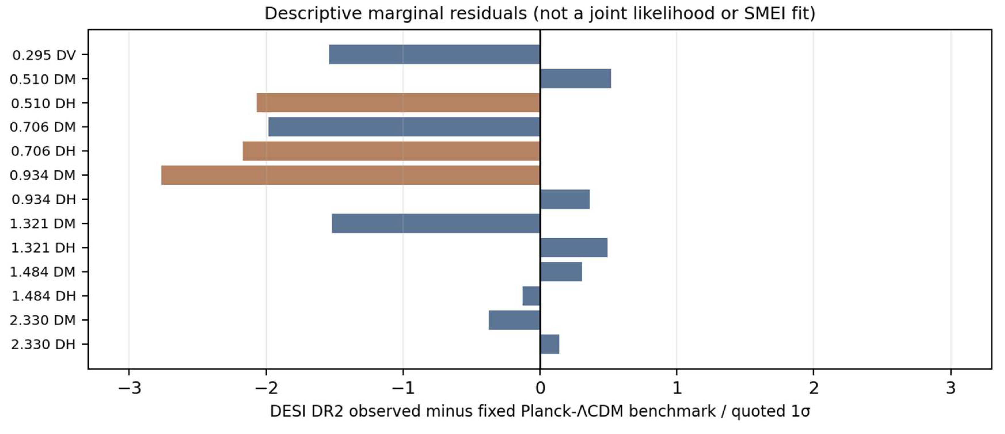
The DESI Collaboration’s DR2 BAO analysis measured geometric distances using more than 14 million galaxies and quasars and combined them with Lyman-α forest results [32,33]. The DR2 sample therefore supplies a more direct redshift-dependent expansion test than simply juxtaposing two H0 estimates. We reproduce 13 published representative BAO values in Table 2, then calculate benchmark predictions from a fixed Planck-consistent flat ΛCDM model, not from SMEI. Use H0,ref = 67.36 km s⁻¹ Mpc⁻¹, Ωm,ref = 0.3153, and rd,ref = 147.09 Mpc [17]. Neglect radiation only for the low-to-moderate redshifts shown. The reference calculation is
The uncertainties sj below are quoted marginal errors from the DESI release, not the full DESI covariance. The qj values are descriptive one-dimensional residuals, not independent significances; multiple rows at the same redshift are correlated, and the benchmark is neither a DESI-only nor a joint best fit.
Figure 2.
Fixed-reference BAO residuals. A subset of individual marginal values is at roughly 2–3 times its quoted standard error, but these numbers cannot be combined as independent evidence against ΛCDM. The published DR2 analysis uses nonzero covariance, parameter fitting and multiple datasets [32]. No SMEI extension has been evaluated in the Figure.
Figure 2.
Fixed-reference BAO residuals. A subset of individual marginal values is at roughly 2–3 times its quoted standard error, but these numbers cannot be combined as independent evidence against ΛCDM. The published DR2 analysis uses nonzero covariance, parameter fitting and multiple datasets [32]. No SMEI extension has been evaluated in the Figure.
The DR2 collaboration’s joint analyses have reported data-combination-dependent preferences for dynamical dark-energy parametrizations over a strict cosmological constant [32]. Such preferences are not a direct observation of mass–energy interconversion: a model must produce a specific H(z), sound horizon, gravitational-growth history and perturbation spectra rather than adopt an arbitrary flexible w0–wa fitting function post hoc. Even an improvement in a phenomenological w0–wa fit would not establish that SMEI generated the observed dynamics.
8.5. What the Data Would Demand From a Proposed SMEI Cosmology
For an operational SMEI-vs-data test, specify ρint(a;θ), pint(a;θ), exchange Q(a;θ), and scalar/vector/tensor perturbations from a common event law. Calculate H(z;θ) and rd(θ) rather than fixing them to Planck when comparing an altered pre-recombination cosmology. Predictions for DM/rd, DH/rd, DV/rd, CMB anisotropy C𝓁, lensing, supernova distance moduli and structure growth must follow. For a complete BAO comparison use
with the official DR2 covariance and consistent treatment of systematic uncertainty. The cosmological event parameters must be constrained using CMB, BAO, Pantheon+, and independent distance-ladder information without double counting shared likelihood components. The full perturbation equations need implementation in a Boltzmann solver and an explicit treatment of calibration/systematic parameters. As of this manuscript, there is no SMEI-specific ySMEI derived from the microscopic model, no published or newly performed SMEI likelihood reanalysis here, and thus no measured reduction of the H0 tension attributable to SMEI.
The observed weak preference in some joint datasets for redshift-dependent dark energy and the discordant Hubble estimates are therefore targets for a predictive model, not observations verifying SMEI. A future model that cannot improve or match the full CMB+BAO+SN fit while also satisfying the interferometric noise restrictions should be rejected in that implementation. Conversely, the ability to fit observations by choosing independent free functions in each domain would not demonstrate the proposed microscopic bridge.
9. Singularities and the Thermodynamic-Pressure Hypothesis
The original essay argued that increasing mass–energy exchanges under compression could generate an outward effective pressure that averts black-hole and big-bang singularities. That is a legitimate question for investigation, but it is not a deduction from the mere presence of positive stochastic pressure. Classical singularity theorems have specific hypotheses about trapped surfaces, causal structure, and energy conditions [15]. Regular-black-hole geometries have been constructed with special stress-energy and horizon properties [16]. SMEI must demonstrate the required stress tensor and its dynamical response rather than presume that any finite-event regulator cures gravitational collapse.
For a spatially flat Friedmann–Lemaître–Robertson–Walker (FLRW) universe in standard Einstein gravity, the Raychaudhuri equation is
A nonsingular bounce at H = 0 with therefore requires ρtot + ptot < 0 in this simple setting; a conventional positive-pressure fluid alone does not suffice. Modified gravity, nonzero curvature, or further dynamical terms can change the conditions, but then they must be exhibited explicitly. A black-hole interior analysis similarly requires a self-consistent metric, regular curvature invariants, stable horizon behavior, and a conservation-respecting effective stress tensor. The claim that stochastic pressure inevitably eliminates singularities should be replaced by this falsifiable mathematical program.
An exploratory parametrization can state pint = pint(ρ,T,) where collects event-rate and correlation invariants. The central tasks are to derive the equation of state, enforce causality and sound-speed bounds, test stability to radial and nonspherical perturbations, and determine whether known energy conditions are broken. These calculations could yield interesting predictions, but they have not been performed in the present manuscript.
10. Time, Thermodynamic Emergence, and the Limits of Interpretation
The stochastic proposal motivates an account of physical change as continual event generation. It may thereby provide an appealing interpretation of temporality and Popper’s interest in indeterminism [4,5,6,28]. Nevertheless, microscopic randomness does not automatically entail a preferred arrow of time. A stationary stochastic process can be statistically invariant under reversal, and macroscopic entropy production depends on dynamics, boundary conditions, coarse-graining, and information flow. An event process should therefore be tested for detailed balance, entropy production, and the relation between microscopic reversibility and macroscopic irreversibility.
Similarly, the philosophical block universe is not straightforwardly falsified by a stochastic matter model. Eternalist and presentist descriptions differ over the ontology of spacetime events; stochastic laws can be represented in mathematical structures that assign probabilities to whole histories. Relativity does not require that every physical process be deterministic. More modestly, SMEI can be interpreted as giving physical significance to open-ended event histories and can motivate discussion of becoming without proving that eternalism is logically inconsistent.
In this sense the philosophical contribution is an organizing principle: physically objective stochastic propensities may coexist with the successful coarse-grained geometry of general relativity, provided the proposed event dynamics has a well-defined relativistic limit. This is a constructive hypothesis; neither a preferred metaphysics nor the language of a ‘thermodynamic engine’ is evidence for its literal operation.
11. Discriminating Predictions and a Falsification Program
A serious falsification program distinguishes internal inconsistency, parameter exclusion, and failure of a necessary signature. The first occurs if no positive, conserved noise law satisfying the stipulated symmetries exists. The second occurs when a specified model parameter region is ruled out. The third occurs when a particular, independently required prediction is absent at adequate sensitivity. The complete SMEI umbrella cannot be decisively falsified by one null visibility experiment unless the umbrella commits to a nonzero, bounded-below noise strength and a fixed correlation structure.
Interferometer protocol. Fix experimental geometries and calculate Kj(t), flight time, arm separation, and environmental decoherence from an established apparatus model. Independently measure the phase-noise spectrum where possible. Fit the differential covariance or its parameterization using Eq. (9) or Eq. (12); include correlated nuisance noise. Compare the Bayesian evidence or likelihood ratios for ordinary quantum/environmental dynamics and SMEI-augmented dynamics, and report confidence or credible intervals on identifiable combinations (typically involving , rather than σΔ and τc separately in the long-time limit). Cross-check at several flight times, masses, momenta, arm separations, and interferometer orientations.
Conservation and laboratory protocol. Any specified coupling capable of exchanging rest energy should predict a compensating channel: recoil, internal energy, emission, or a hidden-sector stress flux. Test energy balance and the absence of unobserved heating or radiation. If the mechanism introduces a particle-species-dependent coupling, compare precision spectroscopy and equivalence-principle constraints. A fit to fringe visibility cannot rescue a microscopic model already incompatible with conservation, positivity, or these independent precision tests.
Cosmological protocol. Implement a concrete ρint(a), w(a), Q(a), and a complete perturbation prescription. Fit to the CMB, baryon acoustic oscillations, supernovae, distance ladders, and large-scale-structure data with consistent priors. Report the change in best-fit likelihood, full parameter uncertainties, model complexity penalty, and shifts in observables besides H0. Avoid using the Hubble tension itself as evidence for an event mechanism. If a shared fundamental parameter is asserted between cosmic sources and laboratory noise, jointly test that same parameter instead of refitting it separately in each domain.
Bell protocol. No independent Bell prediction follows from the present SMEI model. If a future completion claims strict local realism, it must calculate the full conditional distribution P(A,B∣a,b) and explicitly identify why the CHSH derivation does not apply. A claim restricted to common classical noise while retaining Eq. (14) is already excluded by Bell-violating data [10,11,26].
Table 3 summarizes the required logical status of prominent claims.
Table 4 proposes a disciplined experimental matrix. Numerical sensitivities must be taken from the particular instrument and must not be invented from general visibility reports.
12. Discussion: How the Bridge Could Become a Physical Theory
The reconstructed SMEI program is neither empty speculation nor a completed unification. It contains a mathematically transparent family of phase-noise models and a plausible statistical language for stochastic gravitational sources. It has three advantages as a research proposal. First, it separates ensemble mean and residual covariance instead of conflating fluctuations with a gravitational vacuum term. Second, it exposes symmetries and conservation laws as nonnegotiable consistency conditions. Third, it allows interferometry to constrain precisely defined noise correlations rather than vaguely invoking ‘jitter’. The immediate payoff is a sharper test program, not a claim that existing observations select the framework.
Several conceptual trade-offs become visible once the model is written explicitly. A strictly shared time-dependent mass fluctuation is experimentally invisible to a symmetric two-path phase comparison. Increasing spatial decorrelation can yield a signal, but then the physical spatial correlation scale needs explanation. A Lorentz-invariant stress kernel is attractive for gravitation, yet a preferred-time random process is simpler for laboratory phase noise; the bridge cannot assume their equivalence. A short-range event population may coarse-grain smoothly but may not produce the long-range entanglement structure of quantum states. A vacuum-like mean stress tensor can imitate Λ, but its value and radiative stability remain unexplained. Each trade-off is a real scientific constraint and a source of possible theoretical progress.
The comparison with related programs is particularly instructive. Nelson’s stochastic mechanics [7] supplies a diffusion-based route to quantum dynamics, but the identification of its noise with physical mass exchange would require new derivation. Decoherence theory [8] already models loss of interference under environmental coupling; SMEI must predict residual effects not absorbable into conventional environments. Collapse theories [9] are experimentally constrained because they specify noise and modified evolution; SMEI requires comparable operational clarity before comparative statements can be made. Stochastic gravity [13] provides a mature mean/noise formalism; SMEI’s novelty, if established, would concern the microphysical origin and cross-domain constraints of those sources, not the prior existence of the Einstein–Langevin equation. Thermodynamic gravity arguments [12,14] provide useful analogies but do not prove the specific SMEI event mechanism.
A technically adequate next stage would begin with a covariant action for a matter–reservoir system, derive the effective stochastic dynamics after tracing out specified degrees of freedom, and calculate the noise and dissipation kernels together. This must preserve the quantum fluctuation–dissipation relationships when applicable. One should then obtain both an interferometric influence functional and a conserved stress-energy two-point function from common coupling constants. If the same microscopic interaction cannot be shown to account for both, the proposed ‘bridge’ should be understood as a heuristic rather than a unified physical mechanism.
A transparent novelty claim is also essential because the author’s three Applied Physics Research articles are already published [1,2,3]. The present manuscript is a new critical synthesis and conditional extension, not a republication of those papers. Its distinct contributions are the explicit correlation-sensitive visibility equation, the comparison with Bell locality, the conservation/positivity framework, the singularity and Hubble-tension consistency tests, and the cross-domain falsification strategy. Any overlapping equations or prior concepts must remain properly attributed to [1,2,3]; text and graphics should not be reused verbatim without disclosure and applicable permission.
13. Conclusion
Spontaneous subatomic mass–energy interconversion can be organized as a scientifically assessable hypothesis if its stochastic processes, energy-exchange partners, symmetry structure, and observables are specified. Under a weak-noise nonrelativistic approximation, path-dependent inertial-mass fluctuations yield a Gaussian phase-noise visibility formula, but identical noise experienced by identical interferometer arms cancels. Under a marked-event ansatz, mean stress-energy and connected noise can be defined consistently and may enter a stochastic-gravity equation, provided total conservation, covariance, and positivity are enforced. Neither construction alone establishes microscopic diffusion, the Born rule, a solution of the quantum measurement problem, a cosmological constant, a bounce, or an explanation of Bell correlations.
The philosophical significance remains substantial but conditional. A physically meaningful stochastic mechanism would be one possible realization of objective propensity and could help interpret how smooth descriptions arise from microscopic statistics. Its success cannot be inferred from metaphysical appeal. It must earn support by surviving identifiable laboratory and cosmological tests and by avoiding contradiction with the established successes of quantum mechanics and relativity. In that testable, bounded form, stochastic mass–energy interconversion merits investigation as a proposed phenomenological bridge whose future value is determined by calculation and experiment.
Competing interests
Author declares no relevant financial and non-financial interests.
Author Contributions
The author is the sole producer of this work. He claims all conceptualization and approval of all scientific claims.
Funding
Author confirms that no external funding was received.
Data availability
No original experimental measurements, new astrophysical observations, or SMEI-specific likelihood fit are reported. Table 1 and Table 2 transcribe published summary results from the cited articles; Table 2 reference predictions and residuals were newly computed from Eqs. (29)–(30), using published Planck parameters and DESI DR2 marginal errors. Figure 1 and Figure 2 are original plots of those published summary results and calculations. Full instrument-level visibility records and the complete DESI covariance were not downloaded or fitted. Published source URLs and DOIs are listed in the references.
Ethics approval and consent
Not applicable; no research involving human participants or animals is reported.
Use of generative AI
Generative AI assistance was used to structure and draft this manuscript, including explanatory material and mathematical presentation. The author independently verified all scientific derivations, source attributions, citations, originality, and claims, and approved the final text before submission.
Appendix A: Calculation of the Illustrative Gaussian Visibility Law
The displayed interferometric result is worth deriving explicitly because it isolates the assumptions on which the predicted signal depends. For a balanced kinetic-energy profile K and a Gaussian, stationary, mean-zero differential fluctuation Δη(t), let . Being a linear functional of a Gaussian process, X is itself Gaussian and has zero mean. Its variance is
The Gaussian characteristic function gives ⟨eiX⟩ = exp[−Var(X)/2]. Equation (9) immediately follows, with visibility normalized to a calibrated baseline. If CΔ is exponential, symmetry of the double integral permits the reduction
Substitution yields Eq. (10), while Taylor expansion for T/τc≪1 and exponential saturation for T/τc≫1 yield Eq. (11). For a general non-Gaussian process, higher cumulants enter ln⟨eiX⟩; therefore Eqs. (9)–(11) cannot be asserted without specifying Gaussianity or bounding these terms. This distinction matters for a marked-event model, where the underlying statistics may be compound Poisson rather than Gaussian at low event counts.
The same calculation reveals the sensitivity to arm correlations. Suppose η1 and η2 have equal auto-covariance C(τ) and cross-covariance C12(τ) (with a symmetric cross-covariance in the stationary case). Then
CΔ(τ) = 2[C(τ) − C12(τ)]. (A3)
If C12 = C, the noise is common mode and the predicted SMEI phase smearing is exactly absent. If the arms are decorrelated at their separation, C12 → 0 and the full differential variance survives. The distance dependence of C12 is thus one of the most discriminating tests of a spatially correlated mass-noise hypothesis. It should be measured or calculated rather than absorbed into an arbitrary amplitude parameter.
Appendix B: Statistical Exclusion, Null Limits, and Scope of Inference
In a long-duration regime, interferometric data may identify a product such as but not σΔ and τc separately. A model predicting a nonzero lower bound A ≥ A* > 0 can be rejected if the inferred upper bound lies strictly below A* under a pre-specified confidence rule. If the model allows A → 0, a null result excludes only portions of parameter space, not the entire hypothesis. If multiple observables are asserted to share A, their likelihoods should be combined while retaining correlated calibration uncertainties; fitting distinct unrelated A values removes the intended cross-domain test.
A fully specified relativistic event model would require, at minimum, the following mathematical outputs: a matter-plus-reservoir action, a positive event probability measure, conserved total stress-energy for every physically permitted realization (or a justified weaker quantum condition), consistent gauge-fixing and covariance, an observationally admissible source spectrum, and a standard-theory limit. The gravitational source’s covariance should be constrained by transversality, and the noise and response kernel should be derived together when the open-system formulation demands it. The density estimate in Eq. (24) should be linked to a pressure and perturbation system that remains stable. These are necessary publication-quality theoretical milestones, not assertions that the present article has achieved them.
The distinction between consistency, testability, and empirical support also governs the philosophical interpretation. A consistent toy model can illuminate how objective random propensities might operate; a falsifiable extension predicts quantities that could disagree with observation; a supported theory survives sufficiently discriminating independent tests. SMEI at present belongs to the first two categories in the restricted forms derived here. Describing that status precisely is more productive than claiming the ultimate unification of physics before those criteria are met.
Appendix C: Reproducibility of the Published-Data Benchmarks
Interference benchmark. Only the source-reported statement that selected Fein et al. fringe visibilities exceeded 90% of the quantum-theory expectation [21] is used. For a conditional multiplicative attenuation R = exp(−χ), the boundary R = 0.90 produces −ln0.90 = 0.1053605 and, under Gaussian differential-phase assumptions, Var(Δϕ) = 2χ = 0.2107210 rad2. This is an algebraic conversion of a reported visibility ratio, not a 90% (or 95%) statistical confidence level, measurement of mass noise, or estimate of uncertainty about a fitted coupling. To interpret it as a conservative physical SMEI bound would additionally require that ordinary and calibration losses cannot account for the entire shortfall and that the SMEI mechanism can only suppress contrast.
Cosmological reference calculation. DESI values in Table 2 are dimensionless BAO summary measurements [32,33]. For a single intentionally non-refitted comparison, let c = 299792.458 km s⁻¹, H0 = 67.36 km s⁻¹ Mpc⁻¹, Ωm = 0.3153 and rd = 147.09 Mpc. Each tabulated prediction is obtained by numerical quadrature of and the definitions (29)–(30). Predicted ratios are rounded to three decimals; residuals are calculated from the unrounded predictions. Radiation and neutrino corrections to H(z) are omitted in this low-redshift illustrative calculation. For example, at z = 0.295 the observed bright-galaxy DV/rd = 7.942 ± 0.075, while the fixed-reference calculation gives approximately 8.057, a marginal normalized residual of about −1.54. At z = 0.510, DM/rd = 13.588 ± 0.167 compares with a reference near 13.501 (+0.52), and DH/rd = 21.863 ± 0.425 compares with 22.741 (−2.07). A different reference cosmology, propagated Planck uncertainties, the full DR2 covariance, survey systematics, or a likelihood refit changes these residuals. We do not sum their squares or attach a model-selection significance.
No artificial combined constraint. The Planck, ACT, SH0ES, Pantheon+, and DESI summaries overlap in some underlying information or have correlated nuisance structures; in particular ACT’s quoted DR2-combined result reuses DESI and Planck information. Thus the illustrative Planck–SH0ES Gaussian separation is not incorporated as an extra independent data point alongside their parent likelihoods. Tables and figures present an audit of observations and standard-model benchmark calculations, not a statistically independent joint dataset or an SMEI parameter fit.
References
- Willis, R.E. Spontaneous Subatomic Mass-Energy Interconversion: Implications for the Heisenberg Uncertainty Principle and a Theory of Everything. Appl. Phys. Res. 2025, 17(1), 105. [Google Scholar] [CrossRef]
- Willis, R.E. A Dynamical Origin of Wave-Particle Duality From Stochastic Mass-Energy Interconversion. Appl. Phys. Res. 2026, 18(1), 67. [Google Scholar] [CrossRef]
- Willis, R.E. Stochastic Mass-Energy Interconversion as a Bridge From Quantum Noise to Smooth Relativistic Geometry. Appl. Phys. Res. 2026, 18(2), 93. [Google Scholar] [CrossRef]
- Popper, K.R. The Logic of Scientific Discovery; Hutchinson: London, 1959. [Google Scholar]
- Popper, K.R. The propensity interpretation of probability. Br. J. Philos. Sci. 1959, 10(37), 25–42. [Google Scholar] [CrossRef]
- Popper, K. R.: Objective Knowledge: An Evolutionary Approach; Clarendon Press: Oxford, 1972. [Google Scholar]
- Nelson, E. Derivation of the Schrödinger equation from Newtonian mechanics. Phys. Rev. 1966, 150, 1079–1085. [Google Scholar] [CrossRef]
- Zurek, W.H. Decoherence, einselection, and the quantum origins of the classical. Rev. Mod. Phys. 2003, 75, 715–775. [Google Scholar] [CrossRef]
- Bassi, A.; Lochan, K.; Satin, S.; Singh, T.P.; Ulbricht, H. Models of wave-function collapse, underlying theories, and experimental tests. Rev. Mod. Phys. 2013, 85, 471–527. [Google Scholar] [CrossRef]
- Bell, J.S. On the Einstein Podolsky Rosen paradox. Phys. Phys. Fiz. 1964, 1, 195–200. [Google Scholar] [CrossRef]
- Hensen, B.; Bernien, H.; Dréau, A.E.; et al. Loophole-free Bell inequality violation using electron spins separated by 1.3 kilometres. Nature 2015, 526, 682–686. [Google Scholar] [CrossRef]
- Jacobson, T. Thermodynamics of spacetime: the Einstein equation of state. Phys. Rev. Lett. 1995, 75, 1260–1263. [Google Scholar] [CrossRef]
- Hu, B.L.; Verdaguer, E. Stochastic gravity: theory and applications. Living Rev. Relativ. 2008, 11, 3. [Google Scholar] [CrossRef]
- Verlinde, E. On the origin of gravity and the laws of Newton. J. High Energy Phys. 2011, 29, 2011. [Google Scholar] [CrossRef]
- Hawking, S.W. Ellis, G.F.R.: The Large Scale Structure of Space-Time; Cambridge University Press: Cambridge, 1973. [Google Scholar]
- Hayward, S.A. Formation and evaporation of nonsingular black holes. Phys. Rev. Lett. 2006, 96, 031103. [Google Scholar] [CrossRef]
- Planck Collaboration: Planck 2018 results. VI. Cosmological parameters. Astron. Astrophys. 2020, 641, A6. [CrossRef]
- Riess, A.G.; Yuan, W.; Macri, L.M.; et al. A comprehensive measurement of the local value of the Hubble constant with 1 km s−1 Mpc−1 uncertainty from the Hubble Space Telescope and the SH0ES team. Astrophys. J. Lett. 2022, 934, L7. [Google Scholar] [CrossRef]
- Poulin, V.; Smith, T.L.; Karwal, T.; Kamionkowski, M. Early dark energy can resolve the Hubble tension. Phys. Rev. Lett. 2019, 122, 221301. [Google Scholar] [CrossRef]
- Arndt, M.; Hornberger, K. Testing the limits of quantum mechanical superpositions. Nat. Phys. 2014, 10, 271–277. [Google Scholar] [CrossRef]
- Fein, Y.Y.; Geyer, P.; Zwick, P.; et al. Quantum superposition of molecules beyond 25 kDa. Nat. Phys. 2019, 15, 1242–1245. [Google Scholar] [CrossRef]
- Dawid, R. String Theory and the Scientific Method; Cambridge University Press: Cambridge, 2013. [Google Scholar] [CrossRef]
- Weinberg, S. The cosmological constant problem. Rev. Mod. Phys. 1989, 61, 1–23. [Google Scholar] [CrossRef]
- Wald, R.M. General Relativity; University of Chicago Press: Chicago, 1984. [Google Scholar]
- Bohm, D. A suggested interpretation of the quantum theory in terms of “hidden” variables. I. Phys. Rev. 1952, 85, 166–179. [Google Scholar] [CrossRef]
- Clauser, J.F.; Horne, M.A.; Shimony, A.; Holt, R.A. Proposed experiment to test local hidden-variable theories. Phys. Rev. Lett. 1969, 23, 880–884. [Google Scholar] [CrossRef]
- Schlosshauer, M. Decoherence and the Quantum-to-Classical Transition; Springer: Berlin, 2007. [Google Scholar]
- Popper, K.R. The Open Universe: An Argument for Indeterminism; Hutchinson: London, 1982. [Google Scholar]
- Gerlich, S.; Eibenberger, S.; Tomandl, M.; et al. Quantum interference of large organic molecules. Nat. Commun. 2011, 2, 263. [Google Scholar] [CrossRef]
- Eibenberger, S.; Gerlich, S.; Arndt, M.; Mayor, M.; Tüxen, J. Matter-wave interference of particles selected from a molecular library with masses exceeding 10,000 amu. Phys. Chem. Chem. Phys. 2013, 15, 14696–14700. [Google Scholar] [CrossRef]
- Kovachy, T.; Asenbaum, P.; Overstreet, C.; et al. Quantum superposition at the half-metre scale. Nature 2015, 528, 530–533. [Google Scholar] [CrossRef]
- Abdul Karim, M.; et al. (DESI Collaboration): DESI DR2 results. II. Measurements of baryon acoustic oscillations and cosmological constraints. Phys. Rev. D. 2025, 112, 083515. [Google Scholar] [CrossRef]
- Abdul Karim, M.; et al. (DESI Collaboration): DESI DR2 results. I. Baryon acoustic oscillations from the Lyman alpha forest. Phys. Rev. D. 2025, 112, 083514. [Google Scholar] [CrossRef]
- Brout, D.; Scolnic, D.; Popovic, B.; et al. The Pantheon+ Analysis: Cosmological Constraints. Astrophys. J. 2022, 938, 110. [Google Scholar] [CrossRef]
- ACT Collaboration: The Atacama Cosmology Telescope: DR6 power spectra, likelihoods and ΛCDM parameters. J. Cosmol. Astropart. Phys. 2025, 2025(11), 062. [CrossRef]

Table 1.
Data-grounded interferometric benchmarks. Molecular mass in daltons/atomic mass units is not a measured strength of SMEI coupling; models must predict a mass dependence before experiments can exclude them.
Table 1.
Data-grounded interferometric benchmarks. Molecular mass in daltons/atomic mass units is not a measured strength of SMEI coupling; models must predict a mass dependence before experiments can exclude them.
| Publication and apparatus | Published result | What is compared with SMEI | Defensible inference |
|---|---|---|---|
| Gerlich et al. (2011), Kapitza–Dirac–Talbot–Lau [29] | Molecular interference to 6,910 u and 430 atoms | Preservation of coherence in a thermal molecular beam | Extra stochastic dephasing cannot be presumed large; environmental estimates are not an SMEI measurement |
| Eibenberger et al. (2013), molecular grating [30] | Interference beyond 10,000 u and up to 810 atoms | Robustness across molecular mass and structure | Qualitative restriction only without a mass-specific visibility baseline and error model |
| Kovachy et al. (2015), atomic interferometer [31] | Atomic wave packets separated by 54 cm | Dependence of differential noise on path separation | Path separation alone does not establish a noise-amplitude bound |
| Fein et al. (2019), 2-m near-field molecular apparatus [21] | Above 25,000 Da, up to 2,000 atoms; selected fringes >90% of quantum-expected visibility | Relative visibility R = obs/QM in a high-contrast regime | Illustrative upper budget for unmodelled attenuation; not a 95% confidence exclusion |
Table 2.
Actual DESI DR2 BAO measurements [32,33] versus values computed for the fixed flat Planck-reference model defined in Eqs. (29)–(30). Columns are dimensionless. Values have been rounded after numerical integration. These data are not predicted by a completed SMEI cosmology.
| zeff | Tracer; observable | DESI DR2 measured | Planck reference | Difference / quoted 1σ |
|---|---|---|---|---|
| 0.295 | BGS; DV/rd | 7.942 ± 0.075 | 8.057 | -1.54 |
| 0.510 | LRG1; DM/rd | 13.588 ± 0.167 | 13.501 | +0.52 |
| 0.510 | LRG1; DH/rd | 21.863 ± 0.425 | 22.741 | -2.07 |
| 0.706 | LRG2; DM/rd | 17.351 ± 0.177 | 17.702 | -1.98 |
| 0.706 | LRG2; DH/rd | 19.455 ± 0.330 | 20.171 | -2.17 |
| 0.934 | LRG3+ELG1; DM/rd | 21.576 ± 0.152 | 21.996 | -2.76 |
| 0.934 | LRG3+ELG1; DH/rd | 17.641 ± 0.193 | 17.571 | +0.37 |
| 1.321 | ELG2; DM/rd | 27.601 ± 0.318 | 28.084 | -1.52 |
| 1.321 | ELG2; DH/rd | 14.176 ± 0.221 | 14.066 | +0.50 |
| 1.484 | QSO; DM/rd | 30.512 ± 0.760 | 30.278 | +0.31 |
| 1.484 | QSO; DH/rd | 12.817 ± 0.516 | 12.882 | -0.13 |
| 2.330 | Lya-QSO; DM/rd | 38.988 ± 0.531 | 39.186 | -0.37 |
| 2.330 | Lya-QSO; DH/rd | 8.632 ± 0.101 | 8.618 | +0.14 |
Table 3.
Distinction between motivational hypotheses, conditional results, and unresolved theoretical or empirical requirements.
Table 3.
Distinction between motivational hypotheses, conditional results, and unresolved theoretical or empirical requirements.
| Original motivating claim | What the present derivation establishes | What remains to be supplied |
|---|---|---|
| Mass–energy fluctuations underlie quantum uncertainty | A well-defined toy random inertial-mass term, Eq. (1) | A covariant microscopic mechanism reproducing commutators, Born probabilities, and conservation |
| Fluctuations generate wave–particle duality | Conditional Gaussian visibility reduction, Eqs. (6)–(12) | Nonzero differential-noise prediction and exclusion of conventional decoherence |
| A local medium explains Bell entanglement | Bell–CHSH restriction, Eqs. (14)–(15) | A complete Bell-compatible ontology or explicit rejection of an assumption |
| Quantum events generate smooth gravity | A mean/noise decomposition within a metric theory, Eqs. (16)–(22) | A pregeometric derivation and observational gravitational predictions |
| Event fluctuations explain dark energy | Event-rate dimensional estimate, Eq. (24) | Derived equation of state, magnitude, stability, and perturbations |
| The Hubble tension is resolved | A potential sound-horizon route, Eqs. (26)–(27) | Full likelihood fit against multiple datasets |
| Stochastic pressure avoids singularities | Necessary bounce condition, Eq. (32) | Dynamically consistent stress tensor and nonsingular solutions |
Table 4.
A prospective test matrix; entries are proposed future analyses, not completed experimental findings.
Table 4.
A prospective test matrix; entries are proposed future analyses, not completed experimental findings.
| Test | Observable | Differential signature to seek | Principal alternatives or confounders |
|---|---|---|---|
| Molecular or atom interferometry | Visibility as a function of T, K, and arm separation | Spectrally predicted residual from Eq. (12) | Collisions, blackbody radiation, vibrational and laser-phase noise |
| Two-path correlation study | Common-mode versus differential phase | Noise suppression as cross-arm correlation increases | Mechanical common-mode rejection and technical phase locking |
| Precision energy-balance tests | Recoil, spontaneous emission, excess heating | Conserved compensating energy channel tied to noise amplitude | Detector background and ordinary field coupling |
| Stochastic-gravity response | Correlated metric or stress perturbation spectra | Positive, transverse noise kernel with fixed source amplitude | Classical astrophysical and instrumental stochastic backgrounds |
| Cosmological joint fits | CMB peaks, rs, BAO, growth, H0 | Consistent background and perturbation model | Existing EDE, modified gravity, calibration systematics |
| Entanglement measurements | CHSH correlations and no-signalling | Only predictions from a Bell-consistent extension | Standard quantum entanglement |
Disclaimer/Publisher’s Note: The statements, opinions and data contained in all publications are solely those of the individual author(s) and contributor(s) and not of MDPI and/or the editor(s). MDPI and/or the editor(s) disclaim responsibility for any injury to people or property resulting from any ideas, methods, instructions or products referred to in the content. |
© 2026 by the authors. Licensee MDPI, Basel, Switzerland. This article is an open access article distributed under the terms and conditions of the Creative Commons Attribution (CC BY) license (http://creativecommons.org/licenses/by/4.0/).
Copyright: This open access article is published under a Creative Commons CC BY 4.0 license, which permit the free download, distribution, and reuse, provided that the author and preprint are cited in any reuse.