

Submitted:
19 October 2026
Posted:
20 October 2026
You are already at the latest version
Abstract
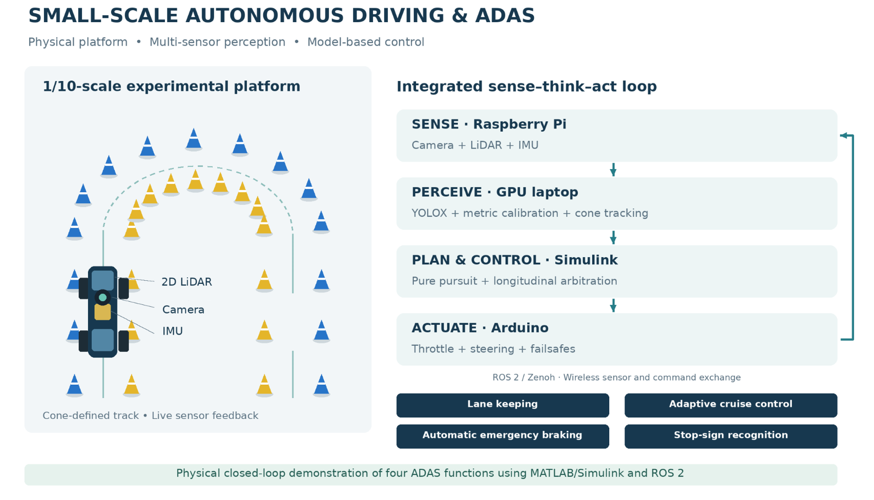
Developing and validating Advanced Driver Assistance Systems (ADAS) on full-size vehicles is expensive, slow and potentially hazardous, which places systematic experimentation out of reach for most students and small research groups. This paper presents the complete design, implementation and experimental evaluation of four ADAS functions—lane keeping, automatic emergency braking, adaptive cruise control and traffic-sign recognition—on a 1/10-scale vehicle, using an industry-standard model-based toolchain built on MATLAB/Simulink and Robot Operating System 2 (ROS 2). The platform combines an on-board Raspberry Pi that streams a 2D Light Detection and Ranging (LiDAR), a fisheye camera and an inertial measurement unit over a Zenoh wireless bridge to a laptop, which runs a You Only Look Once X (YOLOX) cone detector, a camera-to-ground homography, Inertial Measurement Unit (IMU)-LiDAR cone tracking and a Simulink control model, returning drive commands to an Arduino actuation layer. On a Formula-Student-style cone track scaled coherently with the vehicle, the trained detector reaches a mean Average Precision of 0.61 on the boundary cones under the strict Common Objects in Context (COCO) metric, the camera calibration localises cones with a reprojection error of approximately 0.02 m, and the complete perception-planning-control loop runs in real time. The results demonstrate that a transparent, fully model-based ADAS stack can be implemented and validated end-to-end at small scale, providing a low-risk development path toward a full Formula Student Driverless system.
Keywords:
ADAS
; autonomous driving
; small-scale vehicle
; MATLAB/Simulink
; ROS 2
; YOLOX
; sensor fusion
; Formula Student Driverless
1. Introduction
The automotive industry is undergoing a rapid transition from purely human-driven vehicles toward increasingly automated ones. Advanced Driver Assistance Systems such as lane keeping, automatic emergency braking (AEB), adaptive cruise control (ACC) and traffic-sign recognition (TSR) are already widespread in production cars and form the building blocks of the higher levels of driving automation defined by the Society of Automotive Engineers (SAE) standard J3016. Developing and validating these functions on full-size vehicles, however, requires proving grounds, safety drivers and costly instrumentation, which limits how quickly and how often the perception-planning-control loop can be exercised.
Small-scale robotic vehicles have emerged as a recognised alternative: they reproduce the essential sensing, perception and control problems of a real car at a fraction of the cost and risk, and platforms such as F1TENTH [8] and the Formula Student Driverless (FSD) competition have turned scaled autonomy into an established research setting [9,10]. Within this context, the present work asks a practical question: can a representative, integrated set of ADAS functions be implemented and validated on a 1/10-scale vehicle using the same industry-standard, model-based toolchain used in automotive development?
The main contributions of this paper are: (I) a complete, distributed 1/10-scale ADAS platform in which a Raspberry Pi streams sensor data over a Zenoh wireless bridge to a laptop that runs perception, planning and control in MATLAB/Simulink and ROS 2; (II) a perception pipeline that combines a transfer-learned YOLOX cone detector, a fisheye-plus-homography metric calibration and a LiDAR-IMU cone tracker that keeps cone estimates stable when the camera momentarily fails; (III) the implementation of four ADAS functions such as lane keeping by cone-gate pure pursuit, AEB, ACC and stop-sign TSR—integrated into a single fixed-step Simulink model; and (IV) an experimental evaluation covering detection accuracy, metric calibration, real-time behaviour and closed-loop operation, including a practical finding on wireless bandwidth as the dominant source of apparent latency.
2. Related Work
Deep learning now underpins most of the perception stack of automated vehicles; Grigorescu et al. survey its use across scene understanding, planning and control [1]. For object detection, single-stage detectors dominate automotive applications because their single forward pass meets real-time constraints: the You Only Look Once (YOLO) family reformulated detection as regression [2], and YOLOX added an anchor-free, decoupled head that improves the accuracy-latency trade-off [3]. Traffic-sign recognition is a canonical ADAS perception task, with convolutional networks reaching above 99% on the German Traffic Sign Recognition Benchmark (GTSRB) [4].
Localisation without a prior map is addressed by simultaneous localization and mapping (SLAM); Li et al. review LiDAR-based SLAM architectures built from scan matching, loop closure and pose-graph optimisation [5], while Fast LiDAR-Inertial Odometry (FAST-LIO) demonstrates tightly coupled LiDAR-inertial odometry through an iterated extended Kalman filter suitable for small robots [6]. Multi-sensor fusion in the Kalman-filter family remains the standard tool for combining complementary automotive sensors [7].
At small scale, O’Kelly et al. introduced F1/10 as an open-source 1/10 autonomous testbed with a full sensing and software stack [8], and subsequent work standardised evaluation environments and surveyed the methods used on such vehicles, showing how strongly closed-loop performance depends on control rate and localisation quality [9]. The Formula Student Driverless competition defines a standardized cone-marked track: blue cones on the left boundary, yellow on the right, orange at start/finish—and purpose-built datasets such as Formula Student Objects in Context (FSOCO) make the cone-detection problem unusually well supported [10]. On the tooling side, model-based design with MATLAB/Simulink and the ROS 2 middleware [11,12] is exemplified at full scale by Autoware and its Simulink benchmark suite [13,14]. The present work sits at the intersection of these lines: an FSD-style environment, a scaled platform in the F1TENTH tradition, and a fully model-based control stack.
3. System Architecture
Distributed sense-think-act loop. The system is organised as a closed sense-think-act loop distributed across three computers according to their strengths. A Raspberry Pi on the vehicle interfaces with the sensors: an RPLIDAR A1 2D laser scanner, a 160-degree fisheye camera and a Bosch BNO055 inertial measurement unit. The Pi publishes the laser scan (/scan), the compressed camera stream (/image_raw/compressed) and the inertial data (/bno055/imu) as ROS 2 topics, and forwards incoming drive commands over USB serial to an Arduino, which generates the pulse-width modulation (PWM) signals for the electronic speed controller (ESC) and the steering servo. A laptop with a dedicated graphics processing unit (GPU) performs the computationally demanding work—neural-network inference, cone tracking, planning and control—and publishes the drive command (/cmd_drive) back to the vehicle. All control-loop subscriptions use a best-effort, depth-one quality-of-service profile so that consumers always operate on the freshest sample.
Carrying ROS 2 traffic across consumer Wi-Fi with default Data Distribution Service (DDS) multicast discovery proved fragile, so the topics are tunnelled through a Zenoh bridge (zenoh-bridge-ros2dds): a router on each machine is configured with explicit endpoints and forwards only subscribed topics over a single Transmission Control Protocol (TCP) connection. This makes the connection deterministic and efficient without any change to the ROS 2 nodes themselves. The resulting communication graph is shown in Figure 1.
The compute split reflects the platforms: the Raspberry Pi is well suited to sensor and actuator interfacing but cannot run neural-network inference at the required rate, whereas the laptop GPU provides ample headroom. The cost of this split, dependence on the wireless link, is contained by a defense-in-depth safety architecture: the Arduino applies a hardware manual/autonomous switch, a 500 ms serial failsafe and a steering clamp; the Pi forwarder holds a watchdog that outputs neutral if commands stop; the control loop disables motion by default and sends neutral on any exit; and every test begins with the wheels off the ground.
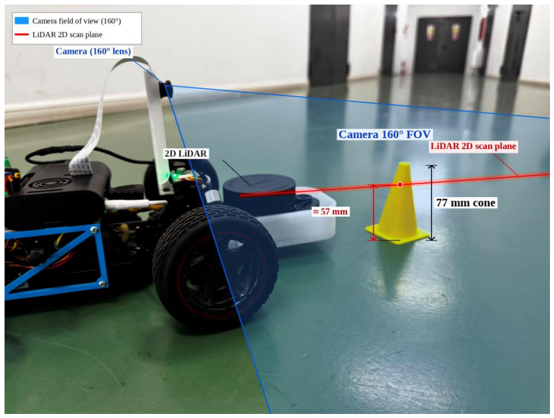
The vehicle is a 1/10-scale (Figure 3) radio-controlled chassis (wheelbase 0.275 m, minimum turning radius 0.5 m, giving a maximum steering angle of approximately 28.8 degrees from the kinematic relation delta_max = arctan(L/R_min)). The track is marked with cones 3D-printed at 77 mm height, one tenth of a standard 762 mm traffic cone, so the entire scene is scaled coherently with the vehicle. Detecting such short cones with a planar scanner requires the scanner to sit low: the LiDAR is mounted at the front with its scan plane approximately 57 mm above the ground, where it intersects the cone bodies, and provides a forward 180-degree field of view. The camera is mounted higher and behind the LiDAR, looking forward over it, which also improves the conditioning of the ground-plane homography used in Section IV (Figure 4).

Table 1.
Main hardware components of the platform.
| Component | Role |
| 1/10 RC chassis (L = 0.275 m) | Mechanical platform, drivetrain, steering |
| Slamtec RPLIDAR A1 (2D) | Planar ranging, forward 180-degree sector |
| 160-degree fisheye camera | Cone and stop-sign detection |
| Bosch BNO055 IMU | Absolute orientation (9-axis fusion) |
| Raspberry Pi (Ubuntu) | Sensor drivers, command forwarder |
| Arduino gateway | PWM to ESC/servo, mode switch, failsafe |
| GPU laptop | Perception, tracking, planning, control |
Figure 2.
Defense-in-depth safety architecture: each layer keeps the vehicle in a safe state even if the layer inside fails.
Figure 2.
Defense-in-depth safety architecture: each layer keeps the vehicle in a safe state even if the layer inside fails.
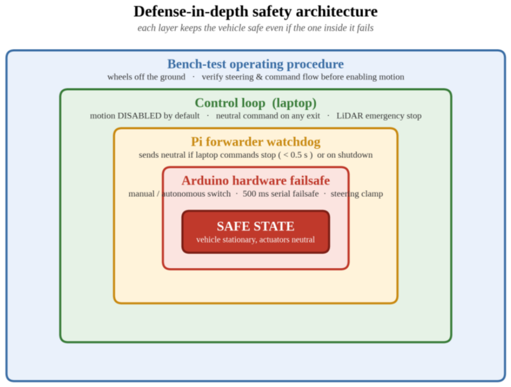
Figure 3.
The experimental platform: 1/10 chassis with the low front LiDAR, raised camera, Raspberry Pi, Arduino gateway and battery.
Figure 3.
The experimental platform: 1/10 chassis with the low front LiDAR, raised camera, Raspberry Pi, Arduino gateway and battery.
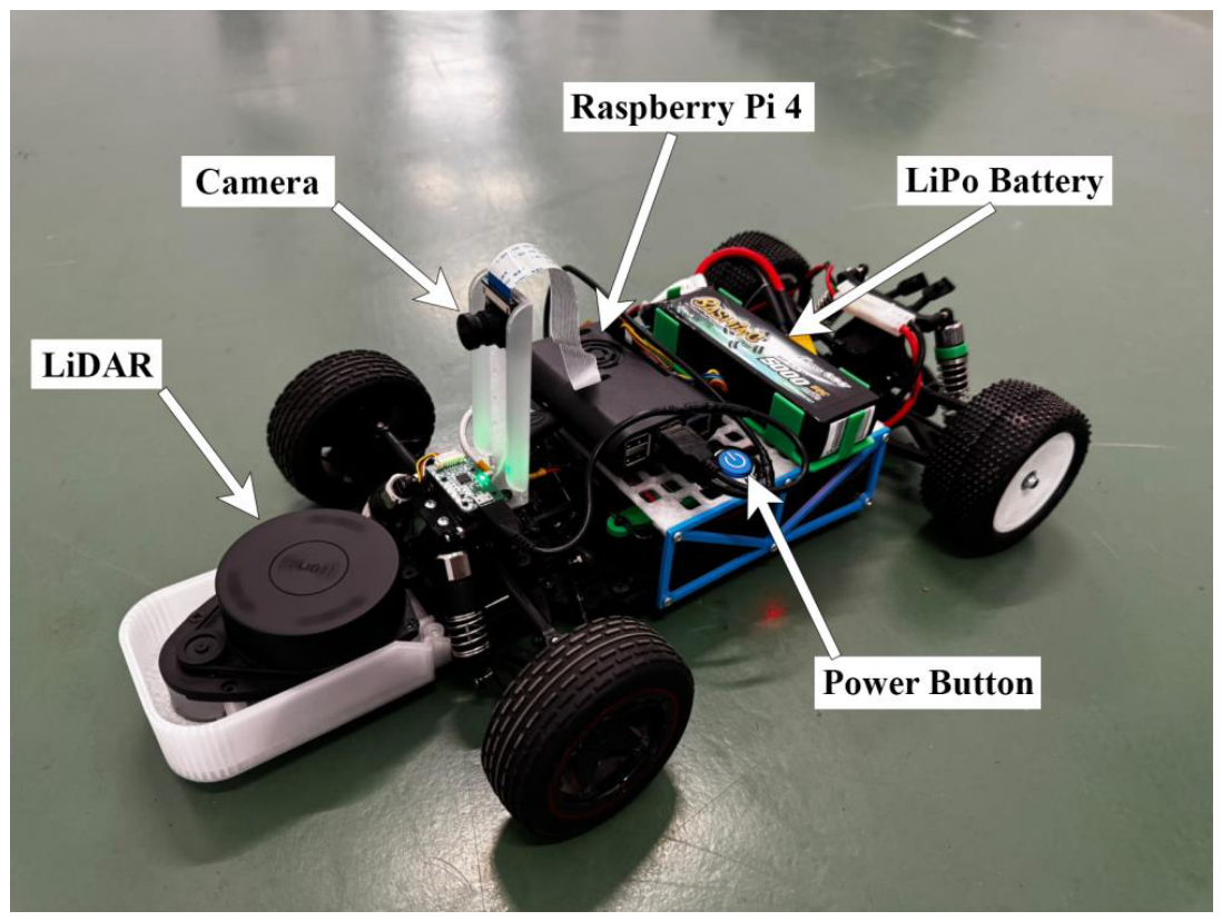
Figure 4.
Sensing geometry: the low front LiDAR scan plane (red, approx. 57 mm) intersects the 77 mm cone, while the raised camera (blue, 160-degree lens) looks forward over the scanner.
Figure 4.
Sensing geometry: the low front LiDAR scan plane (red, approx. 57 mm) intersects the 77 mm cone, while the raised camera (blue, 160-degree lens) looks forward over the scanner.
4. Perception, Planning and Control
The perception of the small-scale vehicle is divided into three directions: cone detection, metric calibration and LiDAR-IMU cone tracking.
Cone detection is performed by a YOLOX single-stage detector [3], chosen for its anchor-free design, real-time speed and native support in the MATLAB toolchain. The detector was produced by transfer learning from a COCO-pretrained YOLOX-small network onto a publicly available Formula Student cone dataset of roughly 3,000 annotated images, expanded by augmentation to approximately 7,300 images and split into 6,430 training, 466 validation and 463 test images at 640x640 pixels, over five classes (blue, yellow, orange, large-orange, unknown). Training ran for twenty epochs on the laptop GPU in approximately eight and a half hours; training and validation losses converged without significant overfitting. A stock COCO-pretrained detector supplies stop-sign detections for the TSR function, gated by a minimum bounding-box area so that only nearby signs trigger a stop.
The planner requires each cone as a metric position in the vehicle frame, not as a bounding box in the image. Two calibrations bridge this gap. First, the 160-degree fisheye lens is calibrated from a set of checkerboard images and each frame is undistorted. Second, a one-time ground-plane homography is estimated from markers placed at measured floor positions: a projective transform maps the pixel at the base of each detection (where the cone meets the floor) to metric ground coordinates (x forward, y left). The perception node applies this transform to every detection, attaches the color class, discards implausible positions and publishes the cone list on /cones as a flat [x, y, colorId] array.
Camera-only cone estimates jitter frame to frame and vanish when a detection is briefly missed, which destabilizes the planner precisely in the situations where accuracy matters most: close cones and tight turns. The pipeline therefore fuses three sources in a lightweight cone tracker. The 2D scan is clustered into small isolated blobs by splitting on Cartesian jumps between consecutive returns; clusters narrower than a cone-width threshold within a trust radius are treated as cone candidates. Camera detections update track color authoritatively; LiDAR clusters update position and, crucially, keep a track alive with its last known color when the camera blinks. The IMU yaw rotates all tracks by the vehicle’s own rotation between updates, preventing mis-association during turns, and an exponential moving average smooths positions. Tracks unseen by both sensors for 0.8 s are dropped. The Simulink model consumes only the fused, stabilized cone list.
The planning and control of the small scale vehicle is divided into: vehicle model and lane keeping, longitudinal functions like AEB, ACC, TSR, and Simulink integration respectively.
Control rests on the kinematic bicycle model: with the rear axle at (x, y), heading theta, wheelbase L and steering angle delta, the vehicle follows dθ/dt = (v/L)·tan(δ), so the instantaneous turning radius is R = L / tan(δ). Lane keeping is a pure-pursuit tracker over the cone-gate centreline: each blue (left) cone is paired with its nearest yellow (right) cone, gate midpoints are sorted by distance ahead and joined into a path, a look-ahead point is selected at distance Ld, and the steering command follows δ = arctan(2L·sin(α) / Ld), where alpha is the bearing to the look-ahead point. When only one boundary colour is visible (the hairpin case) the controller commands full lock away from that boundary (only yellow: full left; only blue: full right), and when no cones are visible it falls back to a LiDAR follow-the-gap behaviour that steers toward the centre of the widest open sector.
Two rate-independent shaping stages remove steering twitch: a first-order low-pass with time constant tau (the command moves a fraction β = Δt / (τ + Δt) toward the target each step) and a slew-rate limit in degrees per second. Because both are parameterised in time units rather than per-step gains, the control rate can be changed without re-tuning the feel.
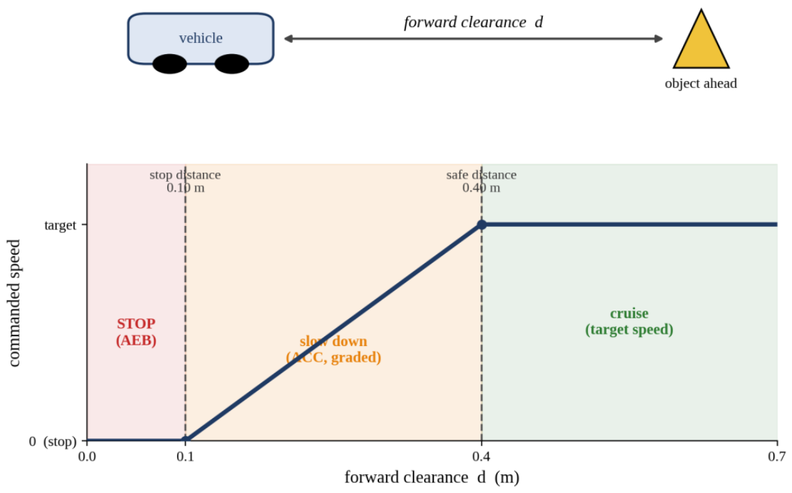
The longitudinal controller arbitrates four behaviours in strict priority: TSR > AEB > ACC > cruise. The forward LiDAR sector is reduced to a minimum-clearance value d. Below a stop distance the commanded speed is zero (AEB); between the stop and safe distances the speed ramps linearly with clearance (ACC); above the safe distance the vehicle cruises at the target speed (Figure 6). A confident, sufficiently close stop-sign detection triggers a stop-hold-resume state machine with a cooldown so the same sign is not re-triggered (TSR). A stall-assist mechanism addresses the ESC dead-band common on hobby hardware: if the controller commands motion but the LiDAR scene does not change, the throttle is ramped in small steps until motion is detected, then held, with the boost reset on any hard stop.
Figure 5.
Kinematic bicycle model: rear-axle reference point, heading, wheelbase L, steering angle and instantaneous centre of rotation.
Figure 5.
Kinematic bicycle model: rear-axle reference point, heading, wheelbase L, steering angle and instantaneous centre of rotation.
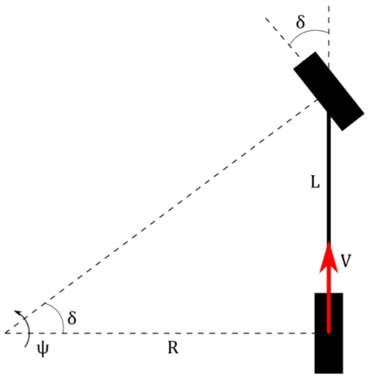
Figure 6.
Longitudinal control law: commanded speed as a function of forward clearance, with the AEB stop zone, the graded ACC zone and the cruise zone.
Figure 6.
Longitudinal control law: commanded speed as a function of forward clearance, with the AEB stop zone, the graded ACC zone and the cruise zone.
The complete controller runs as a single Simulink model built with ROS Toolbox blocks: Subscribe blocks deliver /scan, /cones and /stop_sign as buses, a Planning MATLAB Function block computes the pure-pursuit steering and cone mode, an integrated Controller block combines the lateral and longitudinal laws with the TSR state machine, and the resulting [throttle, steering] command is packed into a std_msgs/Int32MultiArray and published on /cmd_drive. The model uses a fixed-step discrete solver in single-tasking mode and runs in real time against the live sensor streams; motion is disabled by default via an enable constant so the full stack can be exercised safely on the bench. Development followed a port-and-validate strategy: each algorithm was first written and verified as a MATLAB script, then transferred into the model and checked against the script’s behavior.
5. Experimental Results
Cone detection accuracy was evaluated on the held-out test split of 463 images using the COCO protocol, averaging Average Precision (AP) over intersection-over-union (IoU) thresholds from 0.50 to 0.95. Table I reports the per-class results. Orange cones are detected most reliably (AP 0.690), followed by the blue (0.591) and yellow (0.576) boundary cones that define the drivable corridor, and the large-orange start/finish markers (0.573). The ill-defined unknown class—cones that even a human annotator cannot confidently colour, represented by only 178 test objects which scores 0.113, as expected. Excluding this class, which is never used for navigation, the mean Average Precision (mAP) rises from 0.509 to 0.608. These strict-metric values understate practical performance: the planner needs only the projected base of each cone to fall near its true position, not a pixel-perfect box, and at the single 0.5-IoU threshold common in earlier work the scores would be substantially higher.
Table 2.
Per-class Average Precision (COCO IoU 0.50:0.95) of the trained YOLOX cone detector on the test set.
Table 2.
Per-class Average Precision (COCO IoU 0.50:0.95) of the trained YOLOX cone detector on the test set.
| Class | Test objects | AP |
| Orange cone | 955 | 0.690 |
| Blue cone | 2,727 | 0.591 |
| Yellow cone | 2,842 | 0.576 |
| Large orange cone | 199 | 0.573 |
| Unknown | 178 | 0.113 |
| mean AP (all 5 classes) | - | 0.509 |
| mean AP (excl. Unknown) | - | 0.608 |
Regarding the metric calibration accuracy, the fisheye undistortion followed by the ground-plane homography was verified against markers at measured positions: over the 0.4-1.0 m working range in front of the vehicle the mean reprojection error is approximately 0.02 m, so detected cones are localized to within a few centimeters of their true ground position—sufficient for gates roughly 0.5 m wide.
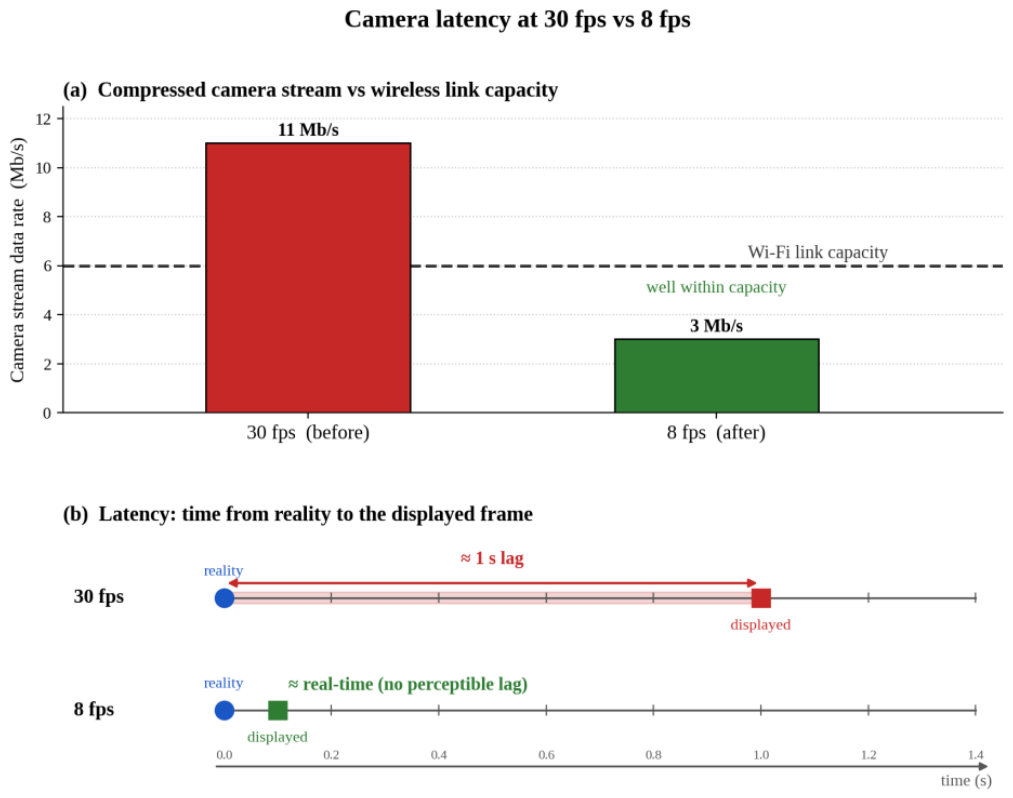
Regarding the real-time behavior and the bandwidth finding, an initial drawback was that the camera view lagged reality by approximately one second while the LiDAR display, crossing the same wireless bridge, remained current. Instrumentation showed that neural-network inference and per-cycle processing each took only tens of milliseconds, so compute was not the cause. The explanation was bandwidth: at 30 frames per second (fps) the compressed video stream saturated the wireless link and accumulated in transit buffers, so every frame arrived fresh from the buffer but old with respect to reality. Reducing the camera to 8 fps brought the stream several-fold below the link capacity and eliminated the delay entirely (Figure 7), while remaining sufficient for the control loop on a slow vehicle. The general lesson is that frame rate and latency are distinct properties, and on a bandwidth-limited link they trade against each other.
With the workload split across processes, the GPU inference on the client, LiDAR SLAM map building on a background worker communicating through a polled data queue, and graphics throttled, the complete perception and visualisation stack holds its rate without stalling, confirming that the earlier bottleneck was MATLAB’s single graphics thread rather than a shortage of compute.
Running on a background worker, the LiDAR SLAM produced a coherent two-dimensional occupancy-grid map of the test environment in real time, streaming snapshots to the operator dashboard without stalling the control loop. Walls and obstacles resolve clearly at the chosen resolution and the estimated trajectory remains consistent through the scene. The reduced forward field of view that follows from the low cone-height mounting offers fewer loop-closure opportunities than a full 360-degree scan, which is the principal mapping limitation of this configuration; for the short forward-driving maneuvers targeted here the local map is sufficient to support obstacle detection and the longitudinal safety functions.
Closed-loop validation: all four functions were exercised in closed loop against live sensors. With both boundary colors in view the planner constructs the centerline and the vehicle follows it by pure pursuit; occluding one color triggers the hairpin full-lock behavior; reducing the forward clearance produces the graded ACC slowdown and, below the stop distance, the AEB stop; presenting a stop sign drives the TSR state machine through stop, hold and resume. The LiDAR-IMU tracker visibly removes the cone flicker and jitter of the camera-only pipeline, and the stall-assist reliably launches the vehicle through the ESC dead-band. The system has thus been demonstrated as a complete loop, from pixels and laser returns to servo pulses, on the physical vehicle.
This paper demonstrated that a representative, integrated ADAS stack: lane keeping, AEB, ACC and traffic-sign recognition; can be implemented and validated end-to-end on a 1/10-scale vehicle using an industry-standard model-based toolchain. The distributed architecture (Raspberry Pi sensing, Zenoh wireless transport, GPU laptop compute, Arduino actuation) proved workable and safe under a layered failsafe design; the perception pipeline achieved 0.61 mAP on boundary cones and 0.02 m metric calibration; and the Simulink controller ran the four functions in real time in closed loop. Beyond the specific results, the platform shows that the perception, fusion and control problems of a driverless race car can be studied, debugged and taught at a fraction of full-scale cost, providing a practical stepping stone toward a complete Formula Student Driverless system.
6. Limitations and Future Work
Three limitations bound the current prototype. First, the cone detector was trained on images from other teams’ cameras and tracks, so a domain gap remains; fine-tuning on frames from the platform’s own camera is expected to raise accuracy. Second, the 2D LiDAR, mounted low to see 77 mm cones, offers only a forward 180-degree view, which limits SLAM loop closure and makes the camera-homography path the primary source of cone positions; its accuracy in turn depends on floor flatness and calibration quality. Third, validation so far covers function-level closed-loop behavior rather than sustained multi-lap driving. Future work therefore targets lap-level evaluation on a full course, extended-Kalman-filter fusion of inertial data with scan-matching odometry for stronger localization, global planning over the SLAM map, and evolution of the platform toward full Formula Student Driverless compliance.
Author Contributions
Conceptualization, C.A.G., B.V. and D.M.; methodology, C.A.G. and D.M.; software, C.A.G.; validation, C.A.G., B.V. and D.M.; formal analysis, C.A.G., B.V. and D.M.; investigation, C.A.G.; resources, C.A.G.; data curation, C.A.G.; writing—original draft preparation, C.A.G., B.V. and D.M.; writing—review and editing, C.A.G. and D.M.; visualization, C.A.G.; supervision, D.M.; project administration, B.V.; funding acquisition, B.V. All authors have read and agreed to the published version of the manuscript.
Data Availability Statement
The data supporting the findings of this study are available from the corresponding author upon request. The publicly available dataset used to train and evaluate the cone detector is described in the manuscript.
Acknowledgments
This research is funded by the European Regional Development Fund (ERDF) through the Smart Growth, Digitalization and Financial Instruments Program, Contract No. 390085/11.11.2025, Project title: Ro-Green—Sustainable Electric Mobility Solutions, SMIS 336225. During the preparation of this manuscript, the authors used Claude Opus (Anthropic; version available in June 2026) to assist with code checking and English language editing. The authors reviewed and edited the output and take full responsibility for the content of this publication.
Conflicts of Interest
The authors declare no conflicts of interest.
Abbreviations
The following abbreviations are used in this manuscript:
| ACC | Adaptive Cruise Control |
| ADAS | Advanced Driver Assistance Systems |
| AEB | Automatic Emergency Braking |
| AP | Average Precision |
| COCO | Common Objects in Context |
| DDS | Data Distribution Service |
| ESC | Electronic Speed Controller |
| FAST-LIO | Fast LiDAR-Inertial Odometry |
| FOV | Field of View |
| fps | Frames per Second |
| FSD | Formula Student Driverless |
| FSOCO | Formula Student Objects in Context |
| GPU | Graphics Processing Unit |
| GTSRB | German Traffic Sign Recognition Benchmark |
| IMU | Inertial Measurement Unit |
| IoU | Intersection over Union |
| LiDAR | Light Detection and Ranging |
| mAP | mean Average Precision |
| PWM | Pulse-Width Modulation |
| RC | Radio-Controlled |
| ROS | Robot Operating System |
| ROS 2 | Robot Operating System 2 |
| SAE | Society of Automotive Engineers |
| SLAM | Simultaneous Localization and Mapping |
| TCP | Transmission Control Protocol |
| TSR | Traffic-Sign Recognition |
| USB | Universal Serial Bus |
| YOLO | You Only Look Once |
| YOLOX | You Only Look Once X |
References
- Grigorescu, S.; Trasnea, B.; Cocias, T.; Macesanu, G. A survey of deep learning techniques for autonomous driving. J. Field Robot. 2020, 37, 362–386. [Google Scholar] [CrossRef]
- Redmon, J.; Divvala, S.; Girshick, R.; Farhadi, A. You only look once: Unified, real-time object detection. In Proceedings of the IEEE Conference on Computer Vision and Pattern Recognition (CVPR), Las Vegas, NV, USA, 27-30 June 2016; pp. 779–788. [Google Scholar] [CrossRef]
- Ge, Z.; Liu, S.; Wang, F.; Li, Z.; Sun, J. YOLOX: Exceeding YOLO series in 2021. arXiv 2021, arXiv:2107.08430. [Google Scholar]
- Arcos-García, Á.; Álvarez-García, J.A.; Soria-Morillo, L.M.; Soria-Morillo, L.M. Deep neural network for traffic sign recognition systems: An analysis of spatial transformers and stochastic optimisation methods. Neural Netw. 2018, 99, 158–165. [Google Scholar] [CrossRef] [PubMed]
- Li, Y.; An, J.; He, N.; Li, Y.; Han, Z.; Chen, Z.; Qu, Y. A review of simultaneous localization and mapping algorithms based on LiDAR. World Electr. Veh. J. 2025, 16, 56. [Google Scholar] [CrossRef]
- Xu, W.; Zhang, F. FAST-LIO: A fast, robust LiDAR-inertial odometry package by tightly-coupled iterated Kalman filter. IEEE Robot. Autom. Lett. 2021, 6, 3317–3324. [Google Scholar] [CrossRef]
- Qian, H.; Wang, M.; Zhu, M.; Wang, H. A review of multi-sensor fusion in autonomous driving. Sensors 2025, 25, 6033. [Google Scholar] [CrossRef] [PubMed]
- O’Kelly, M.; Sukhil, V.; Abbas, H.; Harkins, J.; Kao, C.; Pant, Y.V.; Mangharam, R.; Agarwal, D.; Behl, M.; Burgio, P.; Bertogna, M. F1/10: An open-source autonomous cyber-physical platform. arXiv 2019, arXiv:1901.08567. [Google Scholar]
- Evans, B.D.; Trumpp, R.; Caccamo, M.; Jahncke, F.; Betz, J.; Jordaan, H.W.; Engelbrecht, H.A. Unifying F1TENTH autonomous racing: Survey, methods and benchmarks. arXiv 2024, arXiv:2402.18558. [Google Scholar]
- Vödisch, N.; Dodel, D.; Schötz, M. FSOCO: The Formula Student Objects in Context dataset. SAE Int. J. Connect. Autom. Veh. 2022, 5, 23–32. [Google Scholar] [CrossRef]
- Macenski, S.; Foote, T.; Gerkey, B.; Lalancette, C.; Woodall, W. Robot Operating System 2: Design, architecture, and uses in the wild. Sci. Robot. 2022, 7, eabm6074. [Google Scholar] [CrossRef] [PubMed]
- Quigley, M.; Conley, K.; Gerkey, B.; Faust, J.; Foote, T.; Leibs, J.; Wheeler, R.; Ng, A.Y. ROS: An open-source Robot Operating System. In Proceedings of the ICRA Workshop on Open Source Software, Kobe, Japan, 12 May 2009. [Google Scholar]
- Kato, S.; Tokunaga, S.; Maruyama, Y.; Maeda, S.; Hirabayashi, M.; Kitsukawa, Y.; Monrroy, A.; Ando, T.; Fujii, Y.; Azumi, T. Autoware on board: Enabling autonomous vehicles with embedded systems. In Proceedings of the 2018 ACM/IEEE 9th International Conference on Cyber-Physical Systems (ICCPS), Porto, Portugal, 11-13 April 2018; pp. 287–296. [Google Scholar] [CrossRef]
- Miura, K.; Tokunaga, S.; Ota, N.; Tange, Y.; Azumi, T. Autoware Toolbox: MATLAB/Simulink benchmark suite for ROS-based self-driving software platform. In Proceedings of the 30th International Workshop on Rapid System Prototyping (RSP’19), New York, NY, USA, 17-18 October 2019; Association for Computing Machinery: New York, NY, USA, 2019; pp. 1–7. [Google Scholar] [CrossRef]
- Coulter, R.C. Implementation of the Pure Pursuit Path Tracking Algorithm; Technical Report CMU-RI-TR-92-01; Robotics Institute, Carnegie Mellon University: Pittsburgh, PA, USA, 1992.
- Samuel, M.; Hussein, M.; Mohamad, M.B. A review of some pure-pursuit based path tracking techniques for control of autonomous vehicle. Int. J. Comput. Appl. 2016, 135, 35–38. [Google Scholar] [CrossRef]
- Gafencu, C.-A. MATLAB Simulink-Based Implementation of Autonomous Driving and ADAS Features on a Small-Scale Vehicle. Master’s Thesis, Technical University of Cluj-Napoca, Cluj-Napoca, Romania, 2026. [Google Scholar]
Figure 1.
ROS 2 communication graph: the Raspberry Pi publishes the sensor topics, the perception node publishes /cones, and the Simulink model returns /cmd_drive over the Zenoh bridge.
Figure 1.
ROS 2 communication graph: the Raspberry Pi publishes the sensor topics, the perception node publishes /cones, and the Simulink model returns /cmd_drive over the Zenoh bridge.
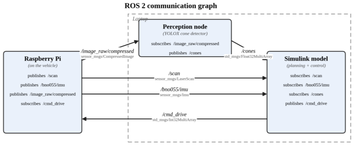
Figure 7.
The bandwidth finding: at 30 fps the compressed stream exceeds the wireless link capacity and the displayed frame lags reality by approx. 1s; at 8 fps the stream fits and the lag disappear.
Figure 7.
The bandwidth finding: at 30 fps the compressed stream exceeds the wireless link capacity and the displayed frame lags reality by approx. 1s; at 8 fps the stream fits and the lag disappear.
Disclaimer/Publisher’s Note: The statements, opinions and data contained in all publications are solely those of the individual author(s) and contributor(s) and not of MDPI and/or the editor(s). MDPI and/or the editor(s) disclaim responsibility for any injury to people or property resulting from any ideas, methods, instructions or products referred to in the content. |
© 2026 by the authors. Licensee MDPI, Basel, Switzerland. This article is an open access article distributed under the terms and conditions of the Creative Commons Attribution (CC BY) license (http://creativecommons.org/licenses/by/4.0/).
Copyright: This open access article is published under a Creative Commons CC BY 4.0 license, which permit the free download, distribution, and reuse, provided that the author and preprint are cited in any reuse.