
Submitted:
19 October 2026
Posted:
20 October 2026
You are already at the latest version
Abstract
This paper proposes a time-varying inertia estimation and economic dispatch method incorporating an inertia safety domain. First, the inertia safety domain is established based on frequency-security constraints and post-contingency inertia availability to determine the admissible inertia range in each period. Second, a fixed-delay online residual physics-informed neural network (Res-PINN) is developed to estimate time-varying inertia and quantify test-set estimation errors. Finally, the estimation error and contingency risk are combined to construct an adaptive inertia margin, which is embedded in a model predictive control dispatch model to dynamically adjust the inertia setting with operating conditions. A 24-h microgrid case study shows that the proposed method achieves zero inertia violations and reduces the average VSG inertia on the system base from 9.8817 s under the fixed-safe strategy to 6.2334 s, demonstrating its effectiveness in maintaining frequency security while reducing inertia redundancy.
Keywords:
islanded microgrid
; inertia safety domain
; virtual synchronous generator
; time-varying inertia estimation
; model predictive control
1. Introduction
In islanded microgrids, distributed energy resources such as wind turbines, photovoltaic units, and energy storage systems are predominantly interfaced through power electronic converters. As the share of synchronous generators decreases, physical inertia declines and frequency-support capability becomes increasingly dependent on operating conditions. Load increases, renewable power drops, or conventional generator outages may cause excessive RoCoF and lower frequency nadirs, potentially leading to frequency violations [1,2]. Inertia and frequency security constraints should therefore be explicitly incorporated into the economic dispatch of islanded microgrids [3].
Virtual synchronous generator (VSG) control is widely applied to energy-storage converters and renewable interfaces to improve frequency dynamics in low-inertia systems [4]. By emulating synchronous-machine rotor dynamics, VSGs provide equivalent inertia and damping and support frequency during the initial disturbance period [5]. In an islanded microgrid containing a diesel generator and wind–solar–storage VSG branches, total inertia comprises the physical inertia of conventional units and the virtual inertia of VSGs. The former is mainly determined by equipment parameters, whereas the latter is adjustable and may vary with operating conditions and control strategies [6,7]. A fixed-inertia assumption therefore fails to reflect time-varying frequency-support capability and may cause either inertia shortages or unnecessary redundancy from persistently high inertia settings [8,9].
Existing inertia-estimation methods mainly include analytical calculation, disturbance-response identification, and data-driven estimation [10,11]. Analytical methods are physically interpretable but sensitive to model parameters and RoCoF measurements. Disturbance-response methods generally require a complete transient process and are therefore more suitable for offline analysis. Purely data-driven methods provide strong nonlinear fitting capability but may yield estimates inconsistent with system frequency dynamics when physical constraints are absent [12]. Physics-informed neural networks (PINNs) incorporate dynamic-equation residuals into training, enabling data fitting while preserving physical consistency and providing an effective approach to online estimation of time-varying inertia [13,14]. Nevertheless, inertia estimates alone cannot guarantee dispatch security. Estimation errors, contingency severity, and frequency-security limits must also be incorporated into the economic dispatch model.
The main contributions are as follows:
(1) Security boundary characterization: An inertia safety domain is established by combining the minimum inertia requirement determined from RoCoF and frequency-nadir constraints with the maximum post-contingency available inertia.
(2) Online inertia estimation: A Res-PINN-based online estimator is developed for time-varying inertia, and its test-set estimation errors are quantified.
(3) Adaptive decision-making: Estimation errors and contingency risks are converted into an adaptive inertia margin and embedded in model predictive control (MPC) dispatch, reducing conservatism while maintaining security.
2. Inertia Safety Domain Modeling for Islanded Microgrids
2.1. Equivalent Inertia and Contingency Model
The dispatch system considered in this study is an islanded microgrid comprising a conventional generator, wind and photovoltaic generation, and a storage-based VSG branch, as shown in Figure 1. The diesel generator provides active-power support and fixed physical inertia, whereas the storage-based VSG provides adjustable virtual inertia and fast frequency support. To incorporate frequency-security requirements into dispatch, an inertia safety domain is constructed to characterize the feasible post-contingency inertia range. Its lower boundary represents the minimum inertia required to satisfy the frequency-security constraints, whereas its upper boundary represents the maximum physically available inertia under the corresponding operating state and contingency.
Since the devices have different rated capacities, their inertia contributions are converted to a common system base. Let , , and denote the system base capacity, conventional-generator capacity, and VSG-branch capacity, respectively, and let and denote their inertia constants. The equivalent system inertia during normal operation in dispatch period is expressed as:
where is the operating-state variable of the conventional generator, equal to 1 when online and 0 otherwise. Equation (1) shows that the equivalent system inertia comprises the physical inertia of the conventional generator and the virtual inertia of the VSG, both converted to the same capacity base. The former is determined by equipment parameters, whereas the latter is adjustable through VSG control and therefore serves as a dispatchable inertia resource.
Different contingencies alter the inertia available after the disturbance. To avoid overestimating frequency support following generator disconnection, the post-contingency available inertia is defined as:
where indicates whether the conventional generator inertia remains available after the contingency. It equals 1 for contingencies other than generator disconnection and 0 when the conventional generator is disconnected. Equation (2) therefore distinguishes the effective inertia support under different contingency types.
The VSG virtual inertia is constrained by its control parameters and storage operating conditions:
Equations (2) and (3) define the post-contingency available-inertia bounds for each period. When the conventional generator remains connected, both physical and virtual inertia contribute to system support. Following generator disconnection, inertia support is provided primarily by the VSG branch. The inertia safety domain therefore depends on the VSG setting, contingency type, and generator operating state.
The inertia safety-domain assessment also requires the maximum active-power imbalance in each period. Because an islanded microgrid lacks support from the upstream grid, load increases, renewable generation drops, and conventional-generator outages may all cause rapid frequency deviations. An extreme contingency power is therefore constructed.
Let PL(k), PW(k), PPV(k), and PG(k) denote the load, available wind power, available photovoltaic power, and conventional-generator output in period k, respectively. The power deficits caused by a load increase, renewable generation reduction, and conventional-generator outage are respectively given by:
where , , and are the load-increase ratio, wind-power-drop ratio, and photovoltaic-power-drop ratio, respectively. The three corresponding power deficits are denoted by , , and . When the conventional generator is offline, and the generator-outage deficit is zero. To represent the most severe operating condition, the largest of the three deficits is selected as the extreme contingency power:
The associated contingency type is recorded to determine whether the physical inertia of the conventional generator remains available. If generator disconnection is the limiting contingency, its physical inertia is excluded from the post-contingency available inertia.
2.2. Minimum Inertia Requirement and Inertia Safety Domain
During the initial stage of a disturbance, the frequency deviation remains small, and RoCoF is mainly determined by the power imbalance and system inertia. To limit the initial frequency decline, the RoCoF constraint should be satisfied [15]:
where is the maximum allowable RoCoF. Based on the relationship between equivalent inertia and RoCoF, the minimum inertia required by the RoCoF constraint is obtained as [16]:
where and denote the nominal frequency and system base capacity, respectively. Equation (9) shows that, for a given RoCoF limit, the minimum inertia requirement increases with the contingency power deficit.
The RoCoF constraint alone cannot fully ensure frequency security because the frequency may continue to decline after the initial disturbance. Therefore, the frequency nadir constraint is also imposed [17]:
where is the frequency nadir following the contingency in period , and is the minimum acceptable frequency. For each contingency, the frequency-nadir constraint is first evaluated at the minimum physically available post-contingency inertia. If the nadir already satisfies (10) at this physical minimum, the frequency-nadir constraint is regarded as inactive and imposes no additional inertia requirement. Otherwise, the minimum inertia satisfying (10) is determined through a one-dimensional search using the reduced-order system frequency-response model. The damping, droop, and response-time parameters used in the frequency-response model are listed in Table A1. Combining the RoCoF and frequency-nadir constraints gives the final minimum inertia requirement:
The RoCoF requirement is governed mainly by the initial power imbalance and equivalent inertia, whereas the frequency nadir also depends on damping and subsequent frequency-response dynamics. The two constraints therefore need not yield the same minimum inertia requirement.
The inertia safety domain can then be constructed for each dispatch period. Its lower boundary is defined by the minimum inertia requirement:
where denotes the lower boundary of the inertia safety domain, representing the minimum post-contingency inertia required to satisfy the RoCoF and frequency-nadir constraints under the limiting contingency.
The upper boundary is determined by the maximum post-contingency available inertia and depends on the contingency type, the VSG inertia limit, and the storage operating state:
where denotes the upper boundary, and is the maximum allowable virtual inertia of the VSG branch. When the limiting contingency is conventional-generator disconnection, its physical inertia is unavailable; otherwise, it remains included in the post-contingency inertia.
The upper boundary represents the physical availability ceiling of inertia rather than a stability-related upper safety limit and does not imply that larger inertia is dynamically unsafe.
Accordingly, the inertia safety domain in period is expressed as:
A feasible domain indicates that the post-contingency frequency-security requirements can be satisfied by adjusting the VSG inertia. If the lower boundary exceeds the upper boundary, the available inertia is insufficient, and additional measures such as increased fast frequency support, revised generator commitment, or greater storage reserve are required.
3. Online Estimation of Time-Varying Inertia
In microgrids with a high penetration of power-electronic devices, storage-based VSGs provide equivalent inertia and damping through their control loops. Because virtual inertia is determined by control parameters and operating conditions, the available frequency support varies over time [18,19,20]. Neural network-based methods have also been applied to continuous and multiarea inertia estimation [21,23].
An online inertia-estimation model is developed using simulated data from a wind–storage VSG microgrid. As shown in Figure 2, frequency and active power responses are measured at the VSG ac terminal upstream of the line impedance. Frequency deviation, active-power disturbance, RoCoF, and time features are then constructed as inputs to the Res-PINN for time-varying inertia estimation.
Online estimation can only use current and historical frequency and power responses. A fixed-delay sliding window is therefore adopted to extract local dynamic features and estimate the inertia at a delayed target instant, as illustrated in Figure 3.
Let denote the sampling instant, the window length, the fixed delay, and the input feature vector. The fixed-delay input window and estimation mapping are expressed as:
where denotes the trainable online Res-PINN, is the input window at time , and is the estimated inertia at the delayed target instant. Because the window contains only current and historical measurements, the estimator satisfies causality. The fixed delay provides a compromise between real-time performance and inertia identifiability.
The input features are derived from frequency and active-power responses and include frequency deviation, active-power disturbance, causally calculated RoCoF, and normalized time describing the relative position within the disturbance process. The feature vector at each sampling instant is:
All features are standardized before being fed into the network. The Res-PINN uses residual blocks to extract temporal dynamics within the input window and outputs the inertia estimate at the target instant [22].
To improve physical consistency, a residual based on the equivalent swing equation is incorporated into training [24]. Neglecting high-frequency electromagnetic transients and retaining the dominant frequency dynamics gives:
where is the time-varying inertia to be estimated and is the equivalent damping coefficient. The corresponding physical residual is:
The training loss is defined as:
where , , and denote the supervised inertia-estimation loss, physical-residual loss, and damping-prior loss, respectively, and , , and are their weights. The physical residual acts as a soft constraint that suppresses estimates inconsistent with the dominant frequency dynamics rather than replacing the detailed microgrid model [25].
The scheduled VSG inertia is a controller setting, whereas the estimator identifies the equivalent inertia reflected in the measured frequency–power response. Because the estimation and dispatch models use different system configurations, the estimated trajectory is not directly imposed on the 24-h dispatch. Instead, the test-set relative-error statistics are used to construct the adaptive inertia margin after all inertia contributions are expressed on the common system base. Thus, the dispatch uses the estimator’s error statistics rather than the estimated inertia trajectory itself.
4. Error-Aware Adaptive-Margin MPC Dispatch Model
4.1. Adaptive Inertia Margin
The lower boundary of the inertia safety domain derived above represents the minimum inertia required for frequency security. To account for online estimation errors, an adaptive inertia margin is added to this lower boundary and incorporated into a receding horizon MPC framework for 24-h economic dispatch [26]. The model takes the load, renewable generation, state of charge (SOC), contingency power, and minimum inertia requirement as inputs and optimizes the conventional generator output, storage power, fast frequency support, and VSG virtual inertia.
The operating risk in each period is first characterized by the limiting contingency power. Let denote the limiting contingency power in period , and let and denote its minimum and maximum values over the dispatch horizon. The risk factor is defined as:
where ρ(k)∈[0, 1] represents the contingency severity in period k. A larger contingency power results in a higher inertia margin.
A relative-error formulation is adopted so that the margin can adapt to different operating conditions. Let denote the baseline relative error and the conservative error bound for high-risk periods. The adaptive error coefficient is defined as:
where and are determined from the test-set MAPE and the 95th percentile of the absolute relative error, respectively. The scheme assigns a more conservative error bound to periods with larger contingency consequences; it does not assume a statistical correlation between contingency power and estimation error.
On the system base, the VSG contribution required to satisfy the basic inertia boundary is:
where is the lower boundary of the inertia safety domain and is the post-contingency available inertia of the conventional generator. Equation (23) gives the inertia contribution that must be supplied by the VSG after subtracting the available physical inertia. When the conventional generator is disconnected, the VSG provides the dominant inertia support.
Based on (22) and (23), the adaptive inertia margin is defined as:
where is an engineering conservatism factor. Because the margin is expressed on the system base, it can be directly included in the MPC inertia constraint. The final inertia requirement for dispatch is therefore:
Equation (25) combines the minimum inertia requirement with the estimation-error margin to form a risk-adaptive dispatch boundary. This avoids applying the maximum inertia setting throughout the day. The corrected boundary is imposed as the MPC inertia-security constraint together with power balance, SOC, ramping, fast-support, and equipment-limit constraints.
4.2. MPC-Based Economic Dispatch Model
After determining the dispatch inertia requirement, a receding horizon optimization model is established based on frequency-constrained economic dispatch [27,28]. At the current dispatch instant , the model predicts over a horizon of periods, implements only the first-period decision, and is solved again in the next period using the updated SOC, load, and renewable generation. The decision variables include conventional-generator output, utilized wind and photovoltaic power, storage charging and discharging power, fast frequency support, SOC, and VSG virtual inertia.
To balance operating economy and frequency security, the objective function includes conventional-generator operating cost, renewable curtailment cost, storage operating cost, fast-support cost, VSG inertia-setting cost, and constraint-violation penalties:
where , , , , , and denote the conventional generator operating cost, renewable curtailment cost, storage operating cost, fast-support cost, VSG inertia-setting cost, and penalty cost, respectively.
Because the islanded microgrid does not exchange power with an upstream grid, the power balance in each period is:
where is the conventional generator output; and are the utilized wind and photovoltaic power, respectively; and are the storage discharging and charging power; and is the load. The utilized wind and photovoltaic power are obtained by subtracting curtailment from the available generation:
The storage SOC evolves according to the charging and discharging power while accounting for standby losses:
The SOC is also subject to operating bounds and a terminal constraint:
where is the rated storage capacity, and are the charging and discharging efficiencies, is the standby-loss coefficient, and is the dispatch interval.
Fast frequency support compensates for the instantaneous post-contingency power deficit. A nonnegative slack variable is introduced to preserve model feasibility under extreme conditions:
where is the available fast-support power and is the required fast support. Fast support represents a second-scale reserve and is therefore excluded from the hourly power-balance equation. The slack variable is assigned a large penalty and remains zero under normal conditions.
The inertia-security constraint is central to the MPC model. The total post-contingency available inertia, comprising the available conventional-generator inertia and the VSG contribution, must satisfy the margin-adjusted dispatch requirement:
where is the post-contingency available inertia of the conventional generator, is the VSG inertia contribution converted to the system base, and is the dispatch inertia requirement including the adaptive margin.
All device powers and the VSG virtual inertia are subject to their respective operating bounds, while the conventional generator output and storage net power satisfy ramp-rate limits. To prevent the VSG inertia setting from exceeding the storage support capability, the effects of SOC and storage-power utilization on the admissible inertia upper bound are further considered:
where is the allowable VSG inertia upper limit at the minimum SOC, is the conversion coefficient between SOC and the inertia limit, and is the reduction coefficient representing the effect of storage-power utilization on the admissible VSG inertia.
5. Case Studies
5.1. Test Systems and Parameter Settings
Simulation data are generated using a wind–storage VSG microgrid model developed in MATLAB/Simulink. The dataset records frequency and active power responses together with the corresponding inertia labels under different inertia trajectories and power disturbances. Each case is simulated from 0.4 to 1.0 s with a sampling interval of 0.01 s, yielding 61 samples. The load disturbance occurs at 0.5 s, and 0.50–0.69 s is selected as the target interval for inertia estimation.
The dataset contains 3000 cases covering constant, step, ramp, sinusoidal, and mixed inertia trajectories. It is divided into training, validation, and test sets at a ratio of 8:1:1. The dataset was divided at the complete-case level, and all sliding windows generated from the same simulation case were assigned to the same subset. The input-window length is , and the fixed delay is , corresponding to an estimation delay of 0.06 s. The test set contains 6000 target points.
LSTM [29] and GRU [30] are selected as benchmark models. All three models use the same data split, input features, target interval, window length, and fixed-delay setting. They are trained for 100 epochs with a batch size of 512 using the AdamW optimizer. The physical-residual loss weight of the Res-PINN is selected according to validation performance and is set to .
The estimation accuracy is evaluated using the root mean square error (RMSE), mean absolute error (MAE), mean absolute percentage error (MAPE), and coefficient of determination (R2):
where and are the actual and estimated inertia at the th test point, respectively; is the mean actual inertia; and is the number of test points. RMSE, MAE, MAPE, and R2 quantify the squared error, absolute error, relative error, and overall goodness of fit, respectively.
A 24-h islanded microgrid comprising a diesel generator, wind and photovoltaic generation, and a storage-based VSG branch is further established to evaluate the proposed adaptive-margin MPC method. The main system parameters are listed in Table A1, while the typical daily load, wind and photovoltaic generation, reference SOC profile used for the inertia safety-domain assessment, and predispatched diesel-generator output are provided in Table A2. The dispatch interval is 1 h, and the prediction horizon is periods. Three strategies are compared: fixed-baseline VSG, fixed-safe VSG, and the proposed time-varying-inertia MPC strategy.
5.2. Inertia Safety-Domain Results
To evaluate the inertia safety domain under time-varying operating conditions, the limiting contingency and corresponding minimum inertia requirement are first determined for each period. The maximum post-contingency available inertia is then evaluated to form the upper boundary, providing the inertia limits for the subsequent dispatch.
As shown in Figure 4, conventional-generator outages cause the largest power deficit in most periods, whereas renewable generation drops become more significant during periods of high photovoltaic output.
Figure 5 shows that the final minimum inertia requirement varies from 3.8000 to 9.0500 s over the 24-h period and reaches its maximum at hour 20. The RoCoF constraint is binding in all periods, whereas the frequency-nadir constraint remains inactive because the nadir limit is already satisfied at the physically admissible minimum inertia. As further verified in Figure 6, the frequency nadir remains above the 49.5 Hz security limit in all periods.
Figure 7 shows that the lower boundary of the inertia safety domain varies with the minimum frequency-security requirement, while the upper boundary is determined by the maximum physically available post-contingency inertia. The domain remains feasible throughout the day, indicating that an admissible inertia configuration exists in every period. The upper boundary represents an inertia-availability ceiling rather than a stability-related maximum safe inertia. The fixed-baseline inertia falls below the lower boundary in most periods, whereas the fixed-safe strategy maintains a conservative inertia level and introduces redundancy during periods with lower requirements.
5.3. Analysis of Online Inertia-Estimation Results
To evaluate the fixed-delay online Res-PINN for time-varying inertia estimation, it is compared with online LSTM and GRU models. All models use the same dataset split, input features, target interval, and fixed-delay window. Their overall test-set performance is summarized in Table 1.
All three models capture the relationship between the frequency–power response and time-varying inertia. Res-PINN performs slightly better across all metrics. Compared with GRU, its MAE decreases from 0.1724 to 0.1464 and its MAPE from 4.33% to 3.55%. The effect of the physical-residual term is further examined through the ablation study below.
Figure 8 shows that the predicted values remain concentrated around the corresponding true inertia levels under the constant-inertia cases.
To assess the effect of the physical-residual term, an ablation study is conducted using different physical-loss weights while keeping the network architecture, data split, and fixed-delay setting unchanged. The results are listed in Table 2, where indicates that the physical-residual constraint is removed.
At , the RMSE, MAE, and MAPE are optimal or nearly optimal. A further increase in the weight imposes an excessively strong simplified swing-equation constraint, which may weaken the model’s ability to fit the nonlinear VSG dynamics. Therefore, is adopted in the subsequent analysis.
Figure 9, Figure 10, Figure 11 and Figure 12 show that Res-PINN effectively tracks step, ramp, sinusoidal, and mixed inertia variations, with the largest errors occurring near abrupt transitions and intervals with superimposed fluctuations. The test-set MAPE is 3.55%, and the 95th percentile of the absolute relative error is 9.19%. These values are used as the baseline and high-risk error coefficients, respectively, in the adaptive inertia-margin formulation. These tests use simulation-generated data; measurement noise, parameter uncertainty, and operating conditions outside the training set are not considered here.
5.4. MPC Dispatch Results and Strategy Comparison
A 24-h typical islanded microgrid scenario with a 1-h dispatch interval is used to validate the proposed method. The lower boundary of the inertia safety domain serves as the basic frequency-security constraint, and the adaptive inertia margin is added to obtain the final MPC inertia requirement.
For the selected typical day, the lower boundary of the inertia safety domain varies from 3.8000 to 9.0500 s. After including the adaptive inertia margin, the inertia requirement imposed on the MPC ranges from 3.9349 to 9.8817 s, while the system-base adaptive margin varies from 0.1052 to 0.8317 s. The dispatch boundary therefore adapts to the operating-risk level instead of using a fixed conservative margin throughout the day.
Three strategies are compared: fixed-baseline VSG, fixed-safe VSG, and the proposed time-varying-inertia MPC. The fixed-baseline strategy uses a low inertia setting, the fixed-safe strategy uses a conservative setting that covers the maximum daily inertia requirement, and the proposed strategy optimizes the VSG virtual inertia in a receding horizon manner. The results are summarized in Table 3.
As shown in Table 3, the fixed-baseline VSG yields the lowest cost but has an inertia violation rate of 95.83% and a maximum inertia deficit of 6.5517 s, and therefore fails to satisfy the frequency-security requirement. The fixed-safe VSG eliminates inertia violations, but its average VSG inertia and average inertia redundancy reach 9.8817 and 3.6483 s, respectively. Under the proposed time-varying-inertia MPC, the inertia violation rate remains zero, while the average VSG inertia decreases to 6.2334 s, representing a 36.92% reduction relative to the fixed-safe strategy. Both the average inertia redundancy and maximum inertia deficit are zero, demonstrating that the proposed method maintains frequency security while suppressing inertia redundancy.
Figure 13 and Figure 14 show that the fixed-baseline VSG remains below the dispatch inertia requirement during most periods, whereas the fixed-safe VSG maintains a consistently high inertia level. By contrast, the proposed method adjusts the post-contingency available inertia according to the time-varying requirement. As the contingency power increases, both the risk factor and adaptive inertia margin increase; during low-risk periods, the margin remains small, thereby reducing inertia redundancy.
Figure 15 and Figure 16 show that the conventional generator, wind and photovoltaic generation, and storage charging/discharging jointly satisfy the load power balance. The storage SOC remains within 0.2500–0.8400, satisfying the prescribed SOC limits.
The total costs of the three strategies differ only slightly. The main advantage of the proposed method is therefore not a substantial reduction in operating cost, but the elimination of inertia violations and the reduction of unnecessary inertia redundancy.
6. Conclusions
This study investigates inertia assessment and security-constrained economic dispatch for an islanded microgrid comprising a conventional generator and wind–solar–storage VSG branches. Following an integrated framework of inertia safety-domain assessment, inertia estimation, and security-constrained dispatch, the main conclusions are as follows:
(1) Frequency security domain assessment: An inertia safety-domain calculation method is established by considering RoCoF, frequency nadir, and post-contingency inertia availability. For the studied daily scenario, RoCoF determines the minimum inertia requirement, while the frequency-nadir constraint remains inactive within the physically admissible inertia range.
(2) Time-varying inertia estimation: A Res-PINN equivalent-inertia estimation method based on a fixed-delay input window is developed, with the frequency-dynamic equation residual embedded in network training. The proposed method achieves lower RMSE, MAE, and MAPE and a higher than LSTM and GRU on the test set. The resulting error statistics are used to construct the inertia margin.
(3) Security-constrained dispatch: An adaptive inertia-margin method considering operating risk is proposed and embedded in the MPC economic dispatch model. The case study shows that, while maintaining a zero inertia-violation rate, the proposed method reduces the average system-base VSG inertia from 9.8817 s (fixed-safe strategy) to 6.2334 s, demonstrating its effectiveness in balancing security and economy.
Author Contributions
Conceptualization, X.N. and Z.N.; methodology, Z.N.; software, Z.N.; validation, Z.N.; formal analysis, Z.N.; investigation, Z.N.; data curation, Z.N.; writing—original draft preparation, Z.N.; writing—review and editing, X.N. and Z.N.; visualization, Z.N.; supervision, X.N.; project administration, X.N.; funding acquisition, X.N. All authors have read and agreed to the published version of the manuscript.
Funding
This research was funded by the National Natural Science Foundation of China, grant number 52367010.
Data Availability Statement
The data presented in this study are available from the corresponding author upon reasonable request.
Conflicts of Interest
The authors declare no conflicts of interest. The funders had no role in the design of the study; in the collection, analyses, or interpretation of data; in the writing of the manuscript; or in the decision to publish the results.
Appendix A
Appendix A.1

Table A1.
Main parameters of the islanded microgrid.
| Category | Parameter | Value | Description |
|---|---|---|---|
| System | Nominal frequency | 50 Hz | Rated system frequency |
| System | System base power | 500 kW | Common power base |
| System | Damping coefficient | 1.5 | Aggregate frequency-damping coefficient used in the SFR model |
| Frequency security | RoCoF limit | 1.0 Hz/s | Maximum allowable rate of change of frequency |
| Frequency security | Frequency-nadir limit | 49.5 Hz | Minimum allowable post-contingency frequency |
| Diesel generator | Rated power | 200 kW | Rated diesel-generator capacity |
| Diesel generator | Inertia constant | 3.5 s | Physical inertia of the diesel generator |
| Diesel generator | Droop coefficient | 0.05 | Speed-governor droop coefficient |
| Diesel generator | Governor time constant | 0.10 s | Time constant of the diesel-generator governor |
| Diesel generator | Engine time constant | 0.30 s | Time constant of the diesel-engine power response |
| VSG | Rated power | 370 kW | Rated capacity of the VSG branch |
| VSG | Baseline virtual inertia | 4.5 s | Fixed-baseline VSG inertia setting |
| VSG | Minimum virtual inertia | 2.0 s | Lower limit of the VSG inertia setting |
| VSG | Maximum virtual inertia | 15.0 s | Upper limit of the VSG inertia setting |
| VSG | Damping coefficient | 25 | Virtual damping coefficient of the VSG controller |
| VSG | Droop coefficient | 0.04 | Active-power–frequency droop coefficient of the VSG |
| VSG | Response time constant | 0.015 s | Response time constant of the VSG active-power support |
| Fast frequency support | Maximum support power | 180 kW | Upper limit of the scheduled fast frequency-support power |
| Contingency coefficient | Load increase | 15% | Proportion of the load-increase contingency |
| Contingency coefficient | Wind-power drop | 20% | Proportion of lost wind generation |
| Contingency coefficient | PV-power drop | 100% | Proportion of lost photovoltaic generation |
| Margin parameter | Baseline relative error | 3.55% | Test-set MAPE of the Res-PINN |
| Margin parameter | High-risk relative-error bound | 9.19% | 95th percentile of the absolute relative error |
| Margin parameter | Engineering conservatism factor | 1.0 | Scaling factor of the adaptive inertia margin |
Table A2.
Operating data for the 24-h typical day.
| Hour | Load (kW) | Wind power (kW) | PV power (kW) | Reference SOC | Predispatched diesel power (kW) |
|---|---|---|---|---|---|
| 1 | 160 | 35 | 0 | 0.65 | 125 |
| 2 | 140 | 48 | 0 | 0.78 | 92 |
| 3 | 118 | 42 | 0 | 0.82 | 76 |
| 4 | 124 | 45 | 0 | 0.82 | 79 |
| 5 | 168 | 52 | 0 | 0.80 | 116 |
| 6 | 187 | 46 | 0 | 0.78 | 141 |
| 7 | 197 | 51 | 1 | 0.75 | 145 |
| 8 | 207 | 55 | 8 | 0.72 | 144 |
| 9 | 228 | 35 | 38 | 0.68 | 155 |
| 10 | 246 | 27 | 78 | 0.62 | 141 |
| 11 | 258 | 22 | 90 | 0.55 | 146 |
| 12 | 267 | 16 | 110 | 0.48 | 141 |
| 13 | 250 | 15 | 101 | 0.42 | 134 |
| 14 | 229 | 23 | 115 | 0.36 | 91 |
| 15 | 210 | 24 | 109 | 0.32 | 77 |
| 16 | 180 | 31 | 87 | 0.30 | 62 |
| 17 | 170 | 41 | 74 | 0.30 | 55 |
| 18 | 189 | 44 | 49 | 0.32 | 96 |
| 19 | 207 | 48 | 18 | 0.35 | 141 |
| 20 | 243 | 58 | 4 | 0.38 | 181 |
| 21 | 229 | 63 | 1 | 0.40 | 165 |
| 22 | 193 | 64 | 0 | 0.42 | 129 |
| 23 | 152 | 62 | 0 | 0.42 | 90 |
| 24 | 130 | 53 | 0 | 0.45 | 77 |
References
- Njoka, G.M.; Mogaka, L.; Wangai, A. Impact of variable renewable energy sources on the power system frequency stability and system inertia. Energy Rep. 2024, 12, 4983–97. [Google Scholar] [CrossRef]
- He, C.; Geng, H.; Rajashekara, K.; Chandra, A. Analysis and control of frequency stability in low-inertia power systems: a review. IEEE/CAA J. Autom. Sin. 2024, 11, 2363–83. [Google Scholar] [CrossRef]
- Zhou, J.; Guo, Y.; Yang, L.; Shi, J.; Zhang, Y.; Li, Y.; et al. A review on frequency management for low-inertia power systems: from inertia and fast frequency response perspectives. Electr. Power Syst. Res. 2024, 228, 110095. [Google Scholar] [CrossRef]
- Shadoul, M.; Ahshan, R.; AlAbri, R.S.; Al-Badi, A.; Albadi, M.; Jamil, M. A comprehensive review on a virtual synchronous generator: topologies, control orders and techniques, energy storages, and applications. Energies 2022, 15, 8406. [Google Scholar] [CrossRef]
- Sang, W.; Guo, W.; Dai, S.; Tian, C.; Yu, S.; Teng, Y. Virtual synchronous generator, a comprehensive overview. Energies 2022, 15, 6148. [Google Scholar] [CrossRef]
- Roy, N.K.; Islam, S.; Podder, A.K.; Roy, T.K.; Muyeen, S.M. Virtual inertia support in power systems for high penetration of renewables—overview of categorization, comparison, and evaluation of control techniques. IEEE Access 2022, 10, 129190–216. [Google Scholar] [CrossRef]
- Jafari, M.; Gharehpetian, G.B.; Anvari-Moghaddam, A. On the role of virtual inertia units in modern power systems: a review of control strategies, applications and recent developments. Int. J. Electr. Power Energy Syst. 2024, 159, 110067. [Google Scholar] [CrossRef]
- Gurski, E.; Kuiava, R.; Perez, F.; Benedito, R.A.S.; Damm, G. A novel VSG with adaptive virtual inertia and adaptive damping coefficient to improve transient frequency response of microgrids. Energies 2024, 17, 4370. [Google Scholar] [CrossRef]
- Ren, B.; Li, Q.; Fan, Z.; Sun, Y. Adaptive control of a virtual synchronous generator with multiparameter coordination. Energies 2023, 16, 4789. [Google Scholar] [CrossRef]
- Kontis, E.O.; Pasiopoulou, I.D.; Kirykos, D.A.; Papadopoulos, T.A.; Papagiannis, G.K. Estimation of power system inertia: a comparative assessment of measurement-based techniques. Electr. Power Syst. Res. 2021, 196, 107250. [Google Scholar] [CrossRef]
- Prabhakar, K.; Jain, S.K.; Padhy, P.K. Inertia estimation in modern power system: a comprehensive review. Electr. Power Syst. Res. 2022, 211, 108222. [Google Scholar] [CrossRef]
- Mazidi, M.; McKelvey, T.; Chen, P. A pure data-driven method for online inertia estimation in power systems using local rational model approach. IEEE Trans. Ind. Appl. 2023, 59, 5506–16. [Google Scholar] [CrossRef]
- Huang, B.; Wang, J. Applications of physics-informed neural networks in power systems—a review. IEEE Trans. Power Syst. 2023, 38, 572–88. [Google Scholar] [CrossRef]
- Yao, W.; Zhao, Y.; Xiong, Y.; Li, Y.; Gan, W.; Wen, J.; et al. Online inertia estimation for wind-integrated power systems with ambient PMU measurements using sliced parallel physics-informed neural networks. Appl. Energy 2026, 414, 127849. [Google Scholar] [CrossRef]
- Chu, Z.; Zhang, N.; Teng, F. Frequency-constrained resilient scheduling of microgrid: a distributionally robust approach. IEEE Trans. Smart Grid 2021, 12, 4914–25. [Google Scholar] [CrossRef]
- Tuo, M.; Li, X. Security-constrained unit commitment considering locational frequency stability in low-inertia power grids. IEEE Trans. Power Syst. 2023, 38, 4134–47. [Google Scholar] [CrossRef]
- Shen, Y.; Wu, W.; Wang, B.; Yang, Y.; Lin, Y. Data-driven convexification for frequency nadir constraint of unit commitment. J. Mod. Power Syst. Clean Energy 2023, 11, 1711–7. [Google Scholar] [CrossRef]
- Liu, D.; Jiang, K.; Ji, X.; Cao, K.; Xu, C.; Sang, S.; et al. Improved VSG strategy of grid-forming inverters for supporting inertia and damping. Front Energy Res. 2024, 11, 1331024. [Google Scholar] [CrossRef]
- Hamanah, W.M.; Shafiullah, M.; Alhems, L.M.; Alam, M.S.; Abido, M.A. Realization of robust frequency stability in low-inertia islanded microgrids with optimized virtual inertia control. IEEE Access 2024, 12, 58208–21. [Google Scholar] [CrossRef]
- Suman, G.K.; Yadav, S.; Guerrero, J.M. Frequency regulation strategy in islanded microgrid with high renewable penetration supported by virtual inertia. Smart Grids Sustain Energy 2024, 9, 33. [Google Scholar] [CrossRef]
- Linaro, D.; Bizzarri, F.; del Giudice, D.; Pisani, C.; Giannuzzi, G.M.; Grillo, S.; et al. Continuous estimation of power system inertia using convolutional neural networks. Nat. Commun. 2023, 14, 4440. [Google Scholar] [CrossRef] [PubMed]
- Zeng, J.; Li, X.; Dai, H.; Zhang, L.; Wang, W.; Zhang, Z.; et al. A residual physics-informed neural network approach for identifying dynamic parameters in swing equation-based power systems. Energies 2025, 18, 2888. [Google Scholar] [CrossRef]
- Poudyal, A.; Tamrakar, U.; Trevizan, R.D.; Fourney, R.; Tonkoski, R.; Hansen, T.M. Multiarea inertia estimation using convolutional neural networks and federated learning. IEEE Syst. J. 2022, 16, 6401–12. [Google Scholar] [CrossRef]
- Stiasny, J.; Chatzivasileiadis, S. Physics-informed neural networks for time-domain simulations: accuracy, computational cost, and flexibility. Electr. Power Syst. Res. 2023, 224, 109748. [Google Scholar] [CrossRef]
- Stiasny, J.; Zhang, B.; Chatzivasileiadis, S. PINNSim: a simulator for power system dynamics based on physics-informed neural networks. Electr. Power Syst. Res. 2024, 235, 110796. [Google Scholar] [CrossRef]
- Fawzy, A.; Bakeer, A.; Magdy, G.; Atawi, I.E.; Roshdy, M. Adaptive virtual inertia-damping system based on model predictive control for low-inertia microgrids. IEEE Access 2021, 9, 109718–31. [Google Scholar] [CrossRef]
- Hu, J.; Shan, Y.; Yang, Y.; Parisio, A.; Li, Y.; Amjady, N.; et al. Economic model predictive control for microgrid optimization: a review. IEEE Trans. Smart Grid 2024, 15, 472–84. [Google Scholar] [CrossRef]
- Wu, Z.; Chen, C.; Xu, D.; Guan, L. Frequency-constrained economic dispatch of microgrids considering frequency response performance. Energies 2025, 18. [Google Scholar] [CrossRef]
- Hochreiter, S.; Schmidhuber, J. Long short-term memory. Neural Comput 1997, 9, 1735–80. [Google Scholar] [CrossRef] [PubMed]
- Mienye, I.D.; Swart, T.G.; Obaido, G. Recurrent neural networks: a comprehensive review of architectures, variants, and applications. Information 2024, 15, 517. [Google Scholar] [CrossRef]
Figure 1.
Configuration of the wind–solar–storage–diesel microgrid.
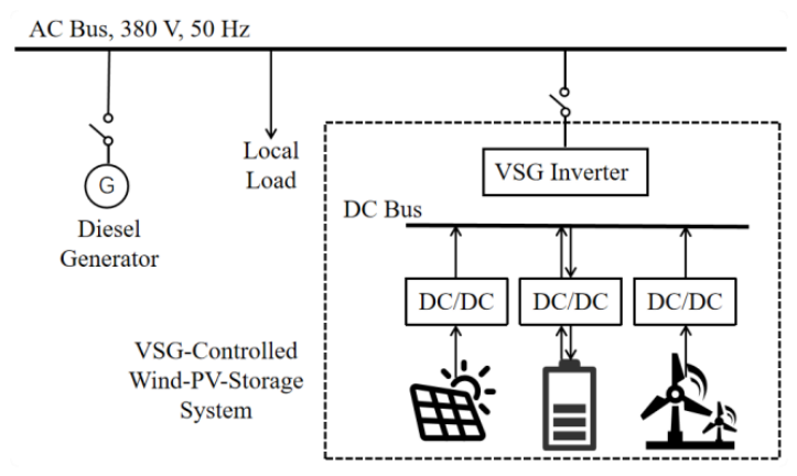
Figure 2.
Wind–storage VSG microgrid and measurement locations.
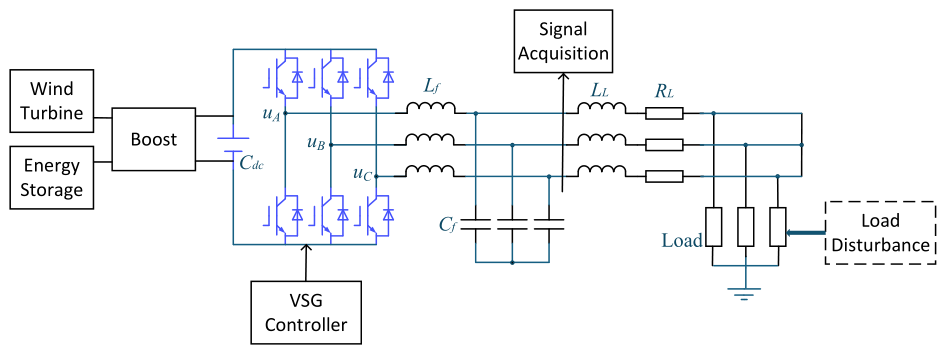
Figure 3.
Online Res-PINN framework for time-varying inertia estimation.
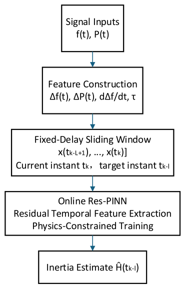
Figure 4.
Comparison of candidate contingency power deficits.
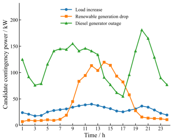
Figure 5.
Minimum inertia requirement under the active frequency-security constraint.
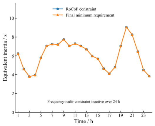
Figure 6.
Frequency-nadir validation at the final minimum inertia requirement.
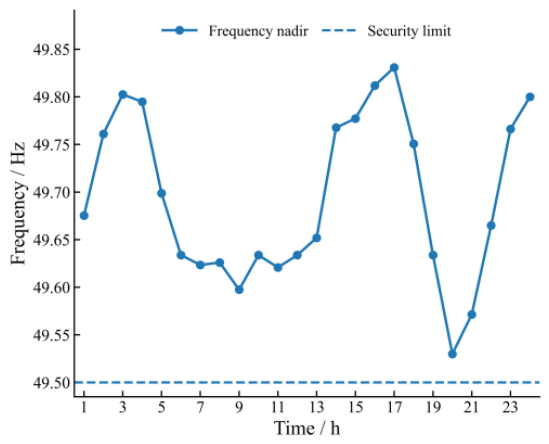
Figure 7.
Inertia safety-domain assessment over 24 h.
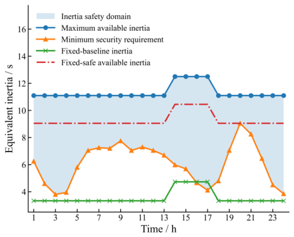
Figure 8.
Test-set prediction distribution under constant-inertia conditions.
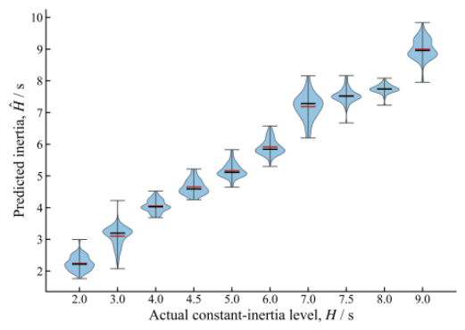
Figure 9.
Actual and estimated inertia under step-inertia conditions: (a) step-inertia case 1; (b) step-inertia case 2.
Figure 9.
Actual and estimated inertia under step-inertia conditions: (a) step-inertia case 1; (b) step-inertia case 2.
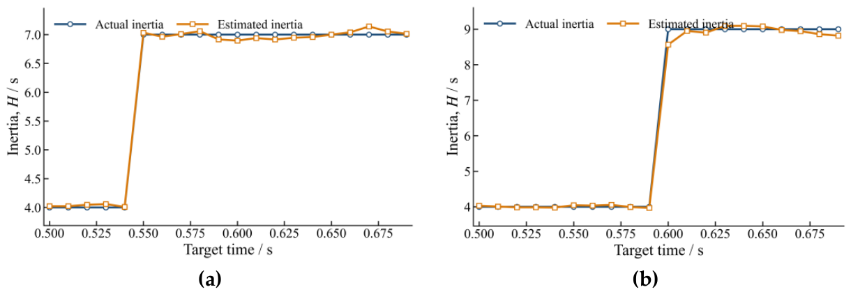
Figure 10.
Actual and estimated inertia under ramp-inertia conditions: (a) ramp-inertia case 1;. (b) ramp-inertia case 2.
Figure 10.
Actual and estimated inertia under ramp-inertia conditions: (a) ramp-inertia case 1;. (b) ramp-inertia case 2.
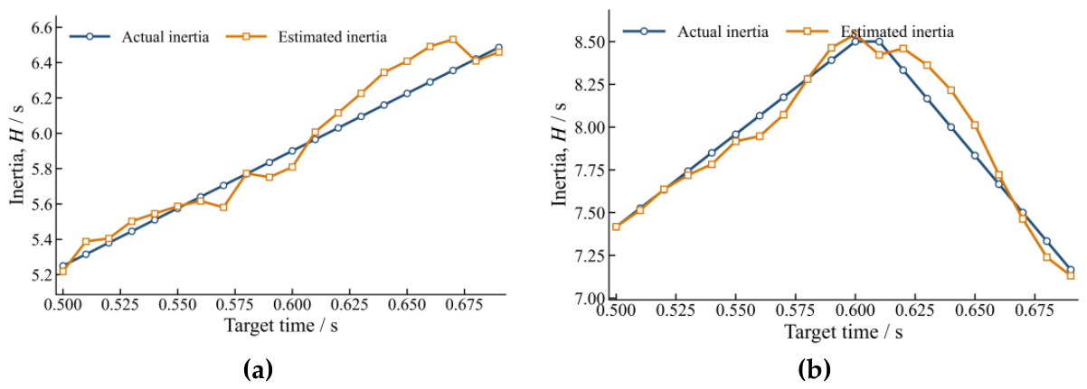
Figure 11.
Actual and estimated inertia under sinusoidal-inertia conditions: (a) sinusoidal-inertia case 1; (b) sinusoidal-inertia case 2.
Figure 11.
Actual and estimated inertia under sinusoidal-inertia conditions: (a) sinusoidal-inertia case 1; (b) sinusoidal-inertia case 2.
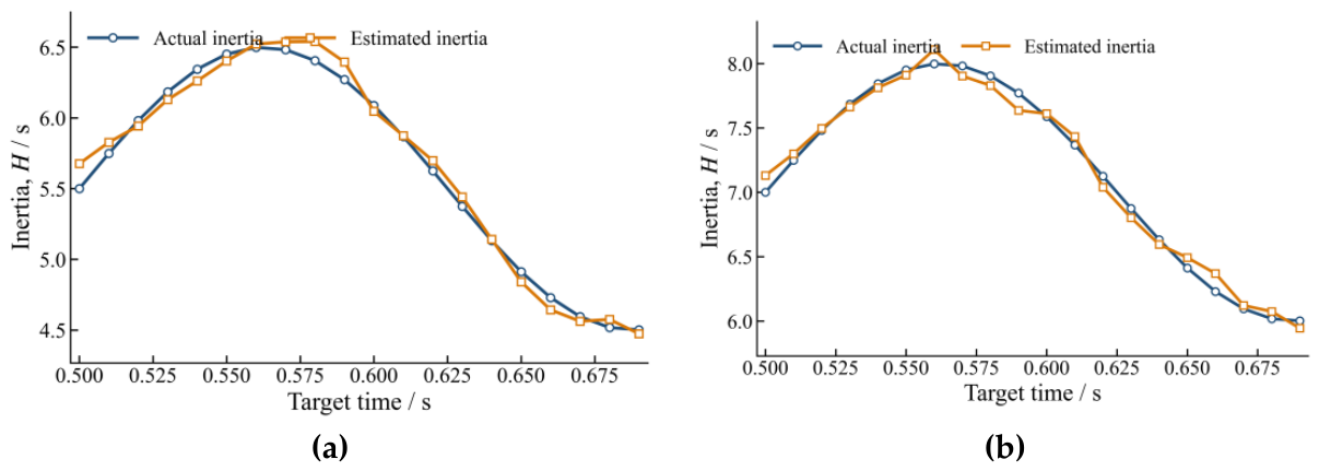
Figure 12.
Actual and estimated inertia under mixed-inertia conditions: (a) mixed-inertia case 1; (b) mixed-inertia case 2.
Figure 12.
Actual and estimated inertia under mixed-inertia conditions: (a) mixed-inertia case 1; (b) mixed-inertia case 2.
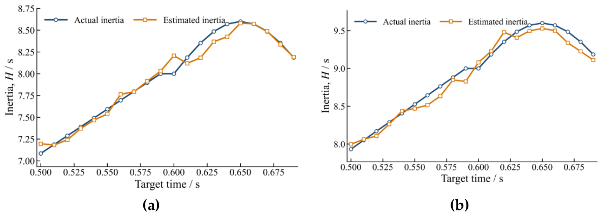
Figure 13.
Comparison of post-contingency available inertia under different strategies.
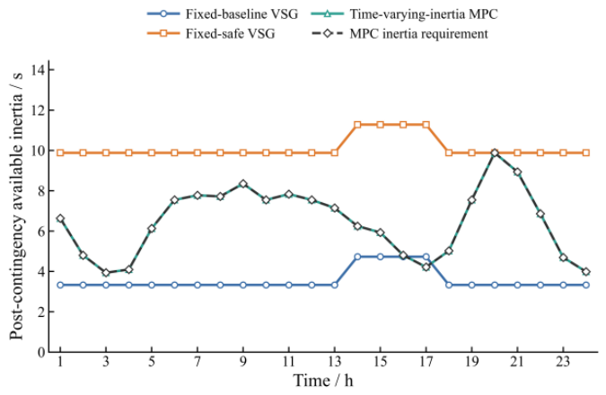
Figure 14.
Adaptive inertia margin and operating-risk factor.
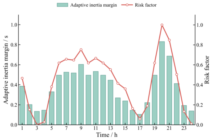
Figure 15.
24-h power-dispatch results under the proposed method.
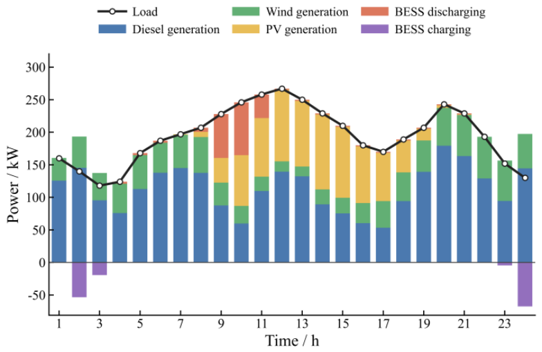
Figure 16.
BESS SOC and net charging/discharging power.
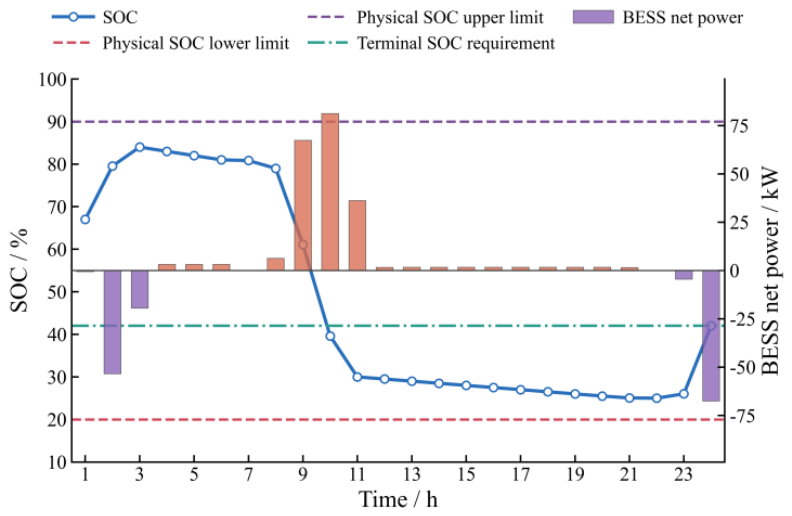
Table 1.
Test-set performance of different online inertia-estimation models.
| Method | RMSE | MAE | MAPE | R2 |
|---|---|---|---|---|
| LSTM | 0.2722 | 0.1773 | 4.52 | 0.9830 |
| GRU | 0.2660 | 0.1724 | 4.33 | 0.9838 |
| Res-PINN | 0.2586 | 0.1464 | 3.55 | 0.9847 |
Table 2.
Test-set performance under different physical-loss weights.
| λphys | RMSE | MAE | MAPE | R2 |
|---|---|---|---|---|
| 0 | 0.2601 | 0.1546 | 3.78 | 0.9845 |
| 0.001 | 0.2599 | 0.1578 | 3.90 | 0.9845 |
| 0.005 | 0.2586 | 0.1464 | 3.55 | 0.9847 |
| 0.01 | 0.2637 | 0.1489 | 3.63 | 0.9840 |
Table 3.
Comparison of different inertia-dispatch strategies.
| Strategy | Total cost (CNY) | Inertia violation rate (%) | Avg. VSG inertia (s) | Avg. total inertia (s) | Avg. inertia redundancy (s) | Max. inertia deficit (s) |
|---|---|---|---|---|---|---|
| Fixed-baseline VSG | 8611.46 | 95.83 | 3.3300 | 3.5633 | 0.0214 | 6.5517 |
| Fixed-safe VSG | 8624.04 | 0.00 | 9.8817 | 10.1150 | 3.6483 | 0.0000 |
| Time-varying-inertia MPC | 8617.03 | 0.00 | 6.2334 | 6.4667 | 0.0000 | 0.0000 |
Note: The VSG inertia values are contributions converted to the system base. Average inertia redundancy includes only the positive margin by which the post-contingency available inertia exceeds the dispatch requirement, whereas inertia shortages are represented separately by the maximum inertia deficit.
Disclaimer/Publisher’s Note: The statements, opinions and data contained in all publications are solely those of the individual author(s) and contributor(s) and not of MDPI and/or the editor(s). MDPI and/or the editor(s) disclaim responsibility for any injury to people or property resulting from any ideas, methods, instructions or products referred to in the content. |
© 2026 by the authors. Licensee MDPI, Basel, Switzerland. This article is an open access article distributed under the terms and conditions of the Creative Commons Attribution (CC BY) license.
Copyright: This open access article is published under a Creative Commons CC BY 4.0 license, which permit the free download, distribution, and reuse, provided that the author and preprint are cited in any reuse.