
Submitted:
19 October 2026
Posted:
20 October 2026
You are already at the latest version
Abstract
The increasing density of wireless communication systems has created new challenges for radio-frequency (RF) security monitoring in critical high security environments, particularly when low-level emissions are in the range of the background noise. This study presents an extended RF spectrum monitoring framework for the detection and analysis of unintended low-level electromagnetic emissions originated from electronic receiver devices. The physical detectability of a characteristic spectral component generated by a tested superheterodyne receiver was evaluated with two different approaches: 1) reference method for RF spectrum analysis: received-power and signal-to-noise ratio (SNR) measurements using a Rohde & Schwarz (R&S) FSH8 spectrum analyzer under different propagation conditions, 2) extended approach: comparison of the radiated RF component with corresponding spectral observations obtained from the protective-earth network, providing an independent conductive measurement domain for spectral cross-validation. Reference-based normalized spectral-similarity metrics were applied to evaluate spectral consistency, while repeated receiver-absent (H_0) and receiver-present (H_1) measurements were used for receiver operating characteristic (ROC) analysis. The effect of linear-power spectral aggregation was further evaluated using bootstrap-based uncertainty analysis with 2000 outer resamples. For the maximum normalized spectral-similarity detector, the direction-oriented area under the ROC curve 〖(S〗_maxAUC) representing detection efficiency increased from 0.6666 to 0.9369 for a single spectrum in 50 aggregated spectra in the 3 m configuration, while smaller or no corresponding aggregation gains were observed under the other investigated measurement configurations (5 and 7 m). The results demonstrate that the received power remains the fundamental physical detection parameter, while spectral similarity, independent cross-domain observation, and statistical validation provide complementary evidence for characterizing persistent low-level receiver-related emissions. The proposed approach provides an experimental basis for extending continuous RF monitoring systems with additional physically interpretable and statistically characterizable detection features for high security environments.
Keywords:
RF spectrum monitoring
; unintended electromagnetic emissions
; superheterodyne receiver
; low-level signal detection
; spectral similarity
; anomaly detection
; RF security
1. Introduction
The increasing density of wireless communication systems has created complex electromagnetic environments characterized by spectral congestion, temporally varying interference, and numerous simultaneously operating RF sources. These conditions present a particular challenge for spectrum monitoring due to the closeness of spectral range of low-level emissions of interest, the local spectral background and/or other wireless systems [1,2]. Consequently, reliable detection cannot be based on received signal level alone, particularly under low-SNR and interference-limited conditions [1,2].
From a security perspective, this issue is relevant to the detection of unauthorized or concealed electronic devices operating within protected environments. Receiver-equipped devices may remain operational without continuously transmitting an intentional communication signal, resulting in conventional monitoring strategies, that are based primarily on active RF transmissions, less effective during receiver-only operation [3]. Detecting low-level unintended emissions associated with active receiver circuitry may therefore provide an additional source of information for security-oriented RF monitoring [3,4].
Electronic receivers nevertheless contain oscillators, mixers, frequency-conversion stages, and other periodically operating circuits capable of generating low-level unintended electromagnetic emissions. In superheterodyne architectures, local-oscillator and frequency-conversion processes can produce receiver-related spectral components that may become observable outside the device under suitable measurement conditions [3,5]. Such emissions are generally substantially weaker than intentional radio transmissions, and their detectability therefore depends on receiver sensitivity, measurement bandwidth, propagation conditions, local interference, and the applied signal-processing method.
Classical spectrum-sensing methods provide several approaches for detecting weak or uncertain RF components. Energy detection offers low implementation complexity when detailed signal information is unavailable, although its performance can degrade at low signal-to-noise ratios and under uncertainty in the local noise level [1,2]. Feature-based, matched, cyclostationary, and correlation-based approaches can exploit additional prior or structural information to improve signal discrimination [1,2]. These principles are relevant to security-oriented RF monitoring because received power provides a direct measure of physical observability, while spectral- and frequency-domain characteristics can provide complementary information regarding the consistency of an observed component with a previously characterized reference.
Recent work has demonstrated that unintended RF emanations can also provide measurable signatures for anomaly-oriented monitoring of electronic systems [6]. Nevertheless, a practical gap remains between conventional signal-presence detection and the characterization of persistent low-level receiver-related emissions using complementary amplitude-, frequency-, spectral-, cross-domain-, and repeated-observation evidence. Signal level alone may provide insufficient evidence when a component approaches the local spectral background or when unrelated signals occupy nearby frequencies. Furthermore, the persistence of receiver-related spectral features under different propagation conditions, their correspondence across independent measurement domains, and the statistical effect of repeated observations require experimental investigation.
The central hypothesis of this study is that a low-level unintended spectral component originated from an operating receiver can be characterized more robustly when received-power information is complemented by spectral similarity, frequency consistency, independent cross-domain observation, and repeated statistical evaluation. Repeated-spectrum aggregation was also investigated for improved statistical separability of persistent low-level spectral structure.
The main contribution of this study is an experimental extension of a conventional signal-level RF monitoring approach toward a multi-evidence framework for low-level unintended receiver-emission detection. Physical detectability was evaluated using received power and local SNR, while reference-based spectral similarity and target-frequency agreement provide complementary descriptors of the observed spectral component. Radiated RF measurements were further compared using an independent conductive-domain observation, and repeated receiver-absent (H0) and receiver-present (H1) measurements. These were evaluated using receiver operating characteristic (ROC) curves and the area under the ROC curve (AUC). Finally, linear-power spectrum aggregation and bootstrap confidence intervals were used to investigate whether repeated observations influence statistical discrimination and to quantify the uncertainty of the estimated aggregation gain.
The study does not attempt to identify the operational purpose of a detected electronic device or to classify a specific threat. Instead, it investigates whether low-level unintended receiver-related emissions can provide additional physically measurable and statistically characterizable features for continuous RF security monitoring. The potential of the approach for future machine-learning-assisted RF anomaly detection was not investigated, no machine-learning classifier was trained or validated in the present study.
2. Materials and Methods
2.1. RF Monitoring Concept and Experimental Objective
The proposed RF monitoring concept is intended to extend the detection capability of continuous spectrum-monitoring systems in high security environments, particularly for low-level RF components that may remain close to the local spectral background. A typical example is an operating receiver-equipped electronic device that does not continuously transmit an intentional communication signal but may generate low-level unintended electromagnetic emissions from active receiver circuitry [3,5].
Figure 1 presents the conceptual architecture of the proposed monitoring framework rather than a fully implemented detection system. Distributed RF sensing nodes continuously observe and monitor the electromagnetic environment and provide spectral data to a central processing layer, which method is based on published work [7,8]. In the proposed RF monitoring concept, this principle is applied to distributed spectrum observations, while the present experimental validation focuses on the feature-extraction and statistical-analysis stages rather than on network-level sensor fusion. The primary detection parameters are received power and local SNR. The proposed extension incorporates additional frequency- and spectral-domain features, repeated statistical evaluation, and, where available, data from an independent measurement domain. Together, these parameters provide a multidimensional representation of the monitored RF environment that may subsequently serve as input to automated anomaly-analysis or machine-learning-assisted RF processing methods [9,10,11].
The experimental objective was therefore to determine whether a low-level unintended spectral component associated with an operating superheterodyne receiver could be physically detected and whether complementary amplitude-, frequency-, and spectral-domain features could be extracted and statistically characterized. The study further investigated whether corresponding spectral evidence could be observed in an independent measurement domain and whether repeated-spectrum aggregation could modify the statistical separability of the extracted spectral features. These experimentally characterized parameters are intended to provide a physical and statistical basis for subsequent automated RF anomaly analysis.
The RF monitoring concept includes a number of physical and statistical methods that provide spectral data and other parameters, which are further explained in detail in the following sections. The step by step description of this extended framework is shown in Figure 2.
2.2. Test Device, Measurement Equipment, and Target Component
A commercially available 433 MHz remote-control receiver module incorporating a superheterodyne architecture was selected as the reference device. The module was used as a reproducible experimental source of low-level unintended receiver-related electromagnetic emissions rather than as a representative of a specific threat device.
Prior to the propagation measurements, the operating receiver was characterized using a near-field magnetic-field probe positioned in close proximity to the receiver circuitry. This preliminary measurement was used to identify a reproducible spectral component associated with receiver operation. A component in the vicinity of 423.26 MHz was observed and selected as the target spectral feature for the subsequent experiments. Because the physical generation mechanism of this component was not independently determined, it is treated throughout this study as a device-specific receiver-related unintended emission rather than being attributed to a particular internal oscillator or frequency-conversion mechanism.
Radiated RF measurements were performed using a Rohde & Schwarz (R&S) FSH8 spectrum analyzer connected to an omnidirectional receiving antenna. The analyzer was configured over a 20 MHz frequency span containing the identified target component. A R&S RTO digital oscilloscope was additionally used for frequency-domain measurements associated with the independent conductive observation channel as described in Section 2.4.
Within each measurement series, the frequency span, resolution bandwidth, detector configuration, and acquisition settings were kept unchanged between the compared measurement states. The acquired spectral data were retained for subsequent received-level, SNR, frequency-consistency, spectral-similarity, and statistical analyses.
2.3. Measurement Environments and Radiated RF Measurement Procedure
The experiment was performed under multiple propagation and electromagnetic conditions to evaluate the detectability of the receiver-related component beyond a single measurement configuration. The primary measurement environment was a furnished office containing typical structural elements, metallic objects, wireless infrastructure, and other active RF sources. These conditions were intentionally retained to provide a practically relevant indoor multipath and interference environment rather than an electromagnetically controlled test configuration.
In the initial measurement setting, the source-to-sensor distance was varied from 0.2 to 7.0 m in increments of 0.1 m. At each position, the received spectrum was recorded using constant analyzer settings during the measurement series. The received spectral level of the detected component around 423.26 MHz and the surrounding local spectral-background level were extracted from each recorded spectrum.
The local SNR at source-to-sensor distance (d) was calculated from the difference between the received target-component level and the estimated local spectral-background level as
where Ptarget is the received target-component level and Pnoise is the estimated local spectral background, both expressed in dBm. Equation (1) represents the difference between two logarithmic power levels, the resulting SNR is expressed in dB.
SNR(d) = Ptarget(d) − Pnoise(d)
For comparison with the measured distance-dependent behavior, the log-distance path-loss model was considered [12]:
where PL(d) is the path loss at source-to-sensor distance d, PL(d0) is the path loss at the reference distance d0, and n is the path-loss exponent. The log-distance formulation provides a simplified reference model for the distance dependence of indoor propagation, while the actual measured levels may additionally be influenced by multipath propagation, shadowing, structural elements, antenna characteristics, and the local electromagnetic environment [12]. For the representation of these types of propagation, n = 3.0 was used in this study, as a representative indoor modelling value rather than as a path-loss exponent estimated from the measurement dataset. The model was therefore used to provide a qualitative propagation reference and not as a fitted predictor of the measured receiver-related emission.
Additional measurements were performed under different propagation conditions, including a comparatively low-external-interference underground environment in which the measurement distance was extended to 20 m. Distance, propagation geometry, multipath conditions, and electromagnetic background were not independently controlled across all configurations, comparisons between environments were interpreted as combined configuration effects rather than as distance-only effects.
2.4. Conductive-Domain Measurement and Cross-Domain Comparison
In addition to the radiated RF measurements, a complementary frequency-domain observation was performed on the protective-earth conductor network using the R&S RTO digital oscilloscope. In this study, the term conductive-domain observation refers to the measurement domain associated with the protective-earth conductor and does not imply that a specific electromagnetic coupling mechanism has been established. The purpose of this measurement was to determine whether a spectral component corresponding in frequency and spectral structure to the receiver-related feature identified in the radiated domain could also be observed through this independent measurement channel.
The radiated and protective-earth measurement paths have different transfer characteristics and were acquired using different measurement configurations, their absolute spectral amplitudes were not directly compared. Instead, the cross-domain analysis focused on frequency correspondence and normalized spectral structure within the target-frequency region. Where numerical comparison required a common frequency grid, the higher-resolution spectrum was interpolated onto the coarser measurement grid. This operation was used solely for frequency-grid alignment and did not increase the physical spectral resolution or information content of any measurements.
The cross-domain analysis was used as an independent spectral-consistency check rather than as a means of identifying the physical coupling path. Observation of corresponding spectral structure in the two measurement domains indicates cross-domain consistency of the measured receiver-related feature, but does not establish whether the underlying coupling is predominantly conductive, capacitive, inductive, radiative, or a combination of these mechanisms. Determination of the physical coupling mechanism would require a dedicated electromagnetic coupling analysis which is beyond the scope of the present study.
2.5. RF Feature Extraction and Spectral Similarity Analysis
To complement received-level and SNR-based detection, additional features (peak spectral level Ppeak, local SNR, zero-lag spectral similarity S0, maximum lag-tolerant spectral similarity Smax, and target-frequency-agreement score Tf) were extracted from each measurement, describing the spectral structure and frequency consistency of the observed receiver-related component. The analysis was restricted to a predefined target-frequency interval centered at f0 = 423.26 MHz with a half-width of 0.10 MHz. Within this interval, each measured spectrum was compared with a reference spectrum representing the previously characterized receiver-related spectral feature.
For the i-th measurement, the feature vector used in the subsequent statistical analysis was defined as
zi = [Ppeak,i,SNRi,S0,i,Smax,i,Tf,i]
Here, Ppeak,i is the maximum measured spectral level within the target interval, SNRi is the corresponding local signal-to-noise ratio, S0,i is the zero-lag spectral-similarity score, Smax,i is the maximum similarity obtained over a restricted set of spectral-sample lags, and Tf,i is the target-frequency-agreement score defined below.
Before spectral-similarity calculation, the median value within the selected target interval was subtracted independently from the measured and reference spectra to reduce the influence of local baseline offsets. Accordingly, and , where xi,k and rk denote the k-th spectral samples of the measured and reference spectra, respectively. Median-based baseline removal was used to reduce sensitivity to local level offsets while avoiding direct dependence of the spectral-shape comparison on the absolute received amplitude.
The zero-lag normalized spectral-similarity score was calculated as
Equation (4) represents a normalized dot-product similarity measure evaluated without frequency-bin displacement. Its value lies between −1 and 1, with larger positive values indicating greater similarity in spectral shape after baseline removal and energy normalization.
To allow for small spectral-grid displacements between the measured and reference spectra, a maximum similarity score was additionally calculated over a restricted set of spectral-sample lags:
Smax,i = Si(l)
Here, Si(l) denotes the normalized spectral similarity evaluated at lag l, and L is the restricted set of allowed spectral-sample lags. In the implemented analysis, the maximum lag parameter was set to one spectral sample; consequently, for target intervals containing a sufficient number of valid samples, the comparison was performed at l = −1,0,+1. The effective lag range was additionally constrained by the number of available samples. For each nonzero lag, only the overlapping portions of the baseline-corrected spectra were compared, and the overlapping segments were independently renormalized to unit energy before the dot product was evaluated.
Frequency consistency was evaluated independently of Smax from the displacement of the measured peak frequency relative to the predefined target frequency f0 = 423.26 MHz. For the i-th measurement, the absolute peak-frequency displacement was defined as
where fpeak,I is the frequency of the maximum measured spectral level within the predefined target interval. In the numerical implementation, ΔfI was expressed in kHz. Smaller values of ΔfI therefore indicate closer agreement with the predefined target frequency.
Δfi = |fpeak,i − f0|
The smaller frequency displacement indicates closer agreement with the predefined target frequency, the displacement was converted to an increasing frequency-match score for ROC analysis as
Tf,i = −Δfi
Thus, larger values of Tf,I represent closer frequency agreement with the target component. This orientation allows the frequency-related feature to be evaluated consistently with the other ROC scores using a decision rule in which larger oriented scores provide increasing evidence for the receiver-present condition.
2.6. Repeated H0/H1 Measurement Protocol and ROC Analysis
To statistically evaluate the discriminative behaviour of the extracted RF features, repeated measurements were acquired under two experiment conditions: H0, corresponding to the receiver-absent state, and H1, corresponding to the receiver-present state. For each investigated measurement configuration, 50 spectra were acquired under H0 and 50 spectra under H1, using the same acquisition settings within the corresponding measurement series.
For every acquired spectrum, the five features defined in Section 2.5 were calculated independently.
ROC analysis was then applied separately to each scalar feature to quantify its ability to discriminate between the two experimentally defined states. For an oriented feature score T and decision threshold τ, the probability of detection was defined as
where a measurement was classified as receiver-present when T ≥ τ.
PD(τ) = P(T ≥ τ|H1)
and the corresponding false-alarm probability was defined as
PFA(τ) = P(T ≥ τ|H0)
The empirical ROC curve was generated by sweeping the decision threshold across the observed feature-score range and calculating the corresponding detection and false-alarm probabilities.
The area under the ROC curve (AUC) was calculated using trapezoidal integration of the empirical ROC points and was used as a threshold-independent measure of feature-level discrimination [8]. An AUC of 0.5 corresponds to chance-level ranking, whereas values approaching 1 indicate increasingly consistent ranking of H1 measurements above H0 measurements. An AUC below 0.5 indicates inverse score ordering rather than an absence of statistical structure [13].
For peak spectral level, SNR, and the frequency-match score Tf, the score definitions were used directly. The raw spectral-similarity scores S0 and Smax were likewise retained without post hoc inversion in the primary single-spectrum ROC comparison. A separate direction-oriented treatment of Smax, used specifically for the repeated-spectrum aggregation analysis, is described in Section 2.7.
2.7. Linear-Power Spectral Aggregation and Bootstrap Uncertainty
To investigate whether repeated observations modify the statistical separability of persistent low-level spectral structure, an additional aggregation analysis was performed on the repeated H0 and H1 measurements. Rather than averaging logarithmic dBm values directly, the measured spectral levels were first converted to linear power before aggregation. This preserves the physical meaning of power averaging and avoids direct arithmetic averaging in the logarithmic domain.
For each frequency sample (f), the spectral level of the (r)-th measurement was converted from dBm to linear power in milliwatts according to
where PdBm,r(f) denotes the measured spectral level at frequency f in the r-th spectrum and PmW,r(f) denotes the corresponding linear power in milliwatts.
For an aggregation size of (R) spectra, the linear-power spectrum was calculated independently at each frequency sample as
where (R) is the number of spectra included in the aggregation. Aggregation sizes of R ∈ 1,5,10,20,30,50 were evaluated representing optimal data size. The H0 and H1 spectra were aggregated separately so that receiver-absent and receiver-present observations were not mixed during spectrum formation. After linear-power aggregation, the resulting mean spectrum was converted back to dBm before calculation of the raw spectral-similarity features S0 and Smax.
For each aggregated spectrum, the maximum normalized spectral-similarity feature Smax was recalculated using the same target interval, reference spectrum, baseline-removal procedure, lag restriction, and normalization rules defined in Section 2.5. ROC analysis was then repeated using the aggregated H0 and H1 similarity scores to determine how the direction-oriented AUC changed as a function of aggregation size (R).
The raw Smax score exhibited inverse ordering in some measurement configurations, therefore a direction-oriented version of the similarity score was used for the aggregation analysis. The score direction was determined once from the corresponding single-spectrum (R = 1) data by comparing the median H0 and H1 scores and was then held constant for all larger aggregation sizes within that measurement configuration. The direction was therefore not re-optimized separately for each value of (R). This procedure preserves a consistent score orientation while allowing aggregation effects to be evaluated relative to the same single-spectrum baseline.
Point estimates on the original measured dataset were obtained using 1000 Monte Carlo aggregation realizations for each aggregation size. These realizations were used to characterize the variability associated with forming aggregated spectra from the finite measurement set and do not contain any additional independent physical measurements.
Uncertainty in the estimated aggregation effect was evaluated using 2000 outer bootstrap resamples [14]. Within each bootstrap replicate, receiver-absent and receiver-present measurements were resampled with replacement within their respective classes, after which the aggregation analysis was repeated using 150 inner Monte Carlo realizations for each aggregation size. This nested procedure produced empirical bootstrap distributions of the AUC at each value of (R) and of the AUC change relative to the corresponding single-spectrum baseline.
To quantify the aggregation effect relative to single-spectrum operation, the AUC change was defined as
ΔAUC(R) = AUC(R) − AUC(1)
Positive values of ΔAUC(R) indicate a higher direction-oriented AUC than the single-spectrum baseline, whereas negative values indicate a lower AUC. For each outer bootstrap replicate, AUC(R) and AUC(1) were obtained from the same resampled H0 and H1 dataset, and their difference was calculated within that replicate. The resulting paired bootstrap distribution therefore preserves the dependence between the aggregated and single-spectrum estimates.
Two-sided 95% percentile confidence intervals for ΔAUC(R) were obtained from the 2.5th and 97.5th percentiles of the paired bootstrap distribution. A confidence interval containing zero was interpreted as indicating that the available measurements did not provide clear evidence of a nonzero aggregation-related AUC change at that aggregation size. Bootstrap and Monte Carlo resampling were used solely to characterize uncertainty and resampling variability and not to increase the number of independent physical observations.
2.8. Data Processing and Reproducibility
All numerical processing and statistical analyses were implemented in MATLAB using R2018b-compatible routines. The analysis was performed directly from the experimentally acquired repeated FSH8 spectra and the corresponding RTO reference spectrum rather than from precomputed feature or ROC tables. This processing chain was used to retain a direct and reproducible relationship between the measured spectral data and the reported statistical parameters.
Before feature extraction, the frequency grids of the repeated H0 and H1 FSH8 measurements were checked for consistency. When the grids were not identical, the H1 spectra were linearly interpolated onto the H0 frequency grid. The higher-resolution RTO reference spectrum was subsequently linearly interpolated onto the FSH8 frequency samples within the predefined target interval. Interpolation was used exclusively for frequency-grid alignment and did not increase the physical spectral resolution or information content of the FSH8 measurements.
The target-frequency interval was centered at f0 = 423.26 MHz with a half-width of 0.10 MHz. For local-background estimation, spectral samples within f0 ± 1.00 MHz were considered while excluding the central f0 ± 0.15 MHz region containing the target component. The local spectral-background level was estimated as the median of the remaining valid spectral samples, and the local SNR was calculated as the difference between the target-band peak level and this median background estimate.
Spectral-similarity processing followed the definitions given in Section 2.5. Within the target interval, the median was removed independently from the measured and reference spectral vectors before unit-energy normalization. The zero-lag score S0 was calculated from the normalized vectors, while Smax was obtained over a maximum displacement of one spectral sample. For nonzero lags, only the overlapping spectral segments were compared and were independently renormalized to unit energy before evaluation of the normalized dot product. The FSH8 frequency spacing was approximately 31.746 kHz, the ±0.10 MHz target interval contained only a limited number of spectral samples; the lag-tolerant comparison was therefore restricted to a maximum displacement of one spectral sample.
Peak-frequency error was calculated relative to the fixed target frequency f0 = 423.26 MHz and expressed in kilohertz. For ROC analysis, the sign of this error was reversed to form the frequency-match score Tf = −Δf, such that larger values represented closer agreement with the predefined target frequency. The extracted feature values were subsequently evaluated using the empirical ROC procedure described in Section 2.6.
For repeated-spectrum aggregation, spectral levels expressed in dBm were first converted to linear power in milliwatts and averaged independently at each frequency sample as described in Section 2.7. The resulting mean spectrum was converted back to dBm before calculation of the raw S0 and Smax spectral-similarity features. Point estimates on the original measured dataset were obtained using 1000 Monte Carlo aggregation realizations for each aggregation size.
For the aggregation analysis, detector orientation was determined once at R = 1 from the original dataset by comparing the median H0 and H1 score ensembles. The resulting direction multiplier (+1 or −1) was then held fixed for all larger aggregation sizes and throughout the bootstrap procedure for the corresponding measurement configuration.
Paired aggregation gains were calculated within the same bootstrap replicate relative to R = 1, and two-sided 95% percentile confidence intervals were obtained from the 2.5th and 97.5th percentiles of the resulting bootstrap distributions. Bootstrap and Monte Carlo resampling were used only to characterize uncertainty and resampling variability and were not interpreted as additional independent physical measurements.
A fixed pseudorandom-number-generator seed of 20260906 was used for the Monte Carlo and bootstrap operations, enabling deterministic reproduction of the reported resampling results from the same input datasets and implementation.
3. Results
3.1. Detection and Signal-Level Characteristics of the Receiver-Related Component
Near-field characterization of the operating receiver revealed a reproducible unintended spectral component in the vicinity of 423.26 MHz. The component was observed during receiver operation and was therefore selected as the target spectral feature for the subsequent radiated measurements. Because the internal physical unintended signal generation mechanism was not independently established, the component is treated here as a device-specific receiver-related unintended emission rather than being attributed to a specific oscillator or frequency-conversion stage.
Figure 3 shows the near-field probe configuration used during the preliminary characterization and the corresponding measured spectral response of the operating receiver. The observed component around 423.26 MHz provided the frequency reference for the subsequent propagation, signal-level, and statistical analyses.
To provide a qualitative propagation reference for the office measurements, the geometry and relevant structural characteristics of the furnished test environment were represented in an indoor propagation simulation. Figure 4 illustrates the resulting spatial variation in the predicted received level for the selected simulation parameters. The simulation was used to visualize the expected influence of the indoor geometry and was not fitted to the measured receiver-related emission data. The simulated field distribution therefore is a propagation reference rather than an experimentally validated radiation pattern of the tested receiver.
Figure 5 illustrates the calculated distance dependence predicted by the log-distance model for different path-loss exponents. Increasing n produces a progressively steeper reduction in predicted received level with distance, illustrating the sensitivity of indoor propagation estimates to the assumed environmental loss factor. For the qualitative comparison used in this study, n = 3.0 was selected as a representative indoor modelling value. This value represents a typical enhanced multi-path, multi-reflection environment and was not estimated by regression from the measured receiver-related emission data.
The furnished office environment was selected as the primary measurement configuration because it represents a practically relevant indoor operating scenario for the proposed monitoring concept. Complementary measurements were additionally performed under different propagation and electromagnetic conditions to examine how the detectability of the receiver-related component changes outside the primary office configuration. The target application area of the proposed system is an indoor furnished office setting in a high security building. Although higher signal levels around the target frequencies were successfully detected in an outdoor environment, that is not a representative target environment. The building structure serves as a spatial separation method to suppress the higher signals coming from outside and consequently this contributes to an improved detection efficiency. These complementary measurements were used to characterize configuration-dependent detectability rather than to establish a universal detection range or threshold.
Figure 6 shows the measurement diagram of the test device placed in an office environment, recorded in a real working, furnished room, near Wi-Fi APs and Bluetooth devices.
The distance-dependent measurements showed a clear overall decrease in received spectral level with increasing source-to-sensor distance. At 0.2 m, the component was typically observed between approximately −60 dBm. At distances of approximately 1–2 m, the received level decreased to the range of −70 to −90 dBm, while beyond 5 m it was generally between approximately −95 and −112 dBm and progressively approached the local spectral background (415-435 MHz, except the target frequency of 423.26 MHz).
The measured distance dependence was not monotonic at every individual position. Local increases and decreases were observed across the measurement series, consistent with the complex propagation conditions of the furnished indoor environment. These variations are therefore interpreted as combined effects of propagation distance, multipath interference, reflections, shadowing, antenna coupling, and the local electromagnetic environment rather than as deviations from an ideal free-space trend.
As the measured target-component level approached approximately - 90 to - 100 dBm in the investigated office configuration, the distinction between the target component and the surrounding local spectral background became progressively less pronounced. This level range is therefore interpreted as an experimentally observed transition region for the present measurement configuration and should not be regarded as a universal receiver-detection threshold.
The spectral evolution shown in Figure 7 further illustrates the progressive reduction in the physical separability of the receiver-related component with increasing distance. The corresponding local SNR exhibited the same general tendency as the received target-component level. At shorter distances, the component remained clearly elevated above the median-based local spectral-background estimate, whereas at larger distances the SNR decreased and became increasingly influenced by local spectral variations.
The SNR follows the same trend as observed in magnitude change as a function of distance between the receiver and the FSH8. The target component was clearly separated from the surrounding spectrum under favourable conditions, whereas reduced signal level resulted in increasing overlap with the local background.
Complementary measurements were performed in an underground environment to characterize the detectability of the receiver-related component under comparatively low external RF activity. Figure 8 shows the measured spectral evolution as a function of source-to-sensor distance up to 20 m. The underground configuration was selected to provide a measurement environment substantially different from the furnished office; however, reflections from the surrounding structural surfaces remained present.
Although the signal-level measurements establish the physical detectability of the receiver-related component, received power alone does not characterize the spectral structure of an observed signal or its statistical relationship to a previously characterized reference. Therefore, the subsequent analysis extends conventional signal-level-based detection by evaluating additional frequency- and spectral-domain features under repeated receiver-absent and receiver-present measurement conditions.
3.2. Statistical Characterization of Complementary RF Features
To extend the signal-level analysis, repeated receiver-absent (H0) and receiver-present (H1) measurements were used to evaluate the complementary RF features defined in Section 2.5. In addition to target-band peak level and local SNR, the evaluated quantities included zero-lag normalized spectral similarity S0, maximum lag-tolerant normalized spectral similarity Smax, and the target-frequency-agreement score Tf. These features characterize complementary amplitude-, spectral-shape-, and frequency-related properties of the measured receiver-related component.
ROC analysis was applied separately to each scalar feature to quantify its single-spectrum discrimination between the experimentally defined H0 and H1 states. The amplitude-based features provided complete ranking separation of the measured H0 and H1 samples under all three investigated configurations. Target-band peak level and local SNR both yielded an AUC of 1.000 at 3 m, 5 m, and 7 m. These values describe the observed feature-level separation within the available measurement dataset and should not be interpreted as evidence of universally perfect detection performance outside the investigated configurations.
The target-frequency-agreement score Tf also showed consistently high discrimination across the investigated configurations, yielding AUC values of 0.920, 0.910, and 0.927 at 3 m, 5 m, and 7 m, respectively. No monotonic reduction in frequency-agreement AUC was observed over these three configurations. The frequency-related feature therefore provided substantial additional separation between the measured H0 and H1 states while remaining distinct from the amplitude-based peak-level and SNR measures.
In contrast, the zero-lag normalized spectral-similarity feature S0 showed comparatively weak single-spectrum discrimination, with AUC values of 0.560, 0.570, and 0.550 at 3 m, 5 m, and 7 m, respectively. The proximity of these values to 0.5 indicates substantial overlap between the H0 and H1 score distributions when individual spectra were evaluated using the zero-lag spectral-similarity metric.
The raw Smax score exhibited inverse ordering under all three investigated configurations, yielding AUC values of 0.348, 0.261, and 0.360 at 3 m, 5 m, and 7 m, respectively. Because the primary single-spectrum analysis retained the original score orientation, AUC values below 0.5 indicate inverse ordering of the H0 and H1 score distributions for the selected reference spectrum rather than, by themselves, an absence of statistical structure. No post hoc inversion was applied to the raw Smax values in this primary feature comparison.
Figure 9 presents the representative ROC analysis for the 3 m configuration, while Table 1 summarizes the AUC values obtained at all three investigated distances (3, 5 and 7m). Within the available measurements, target-band peak level and local SNR provided the strongest individual feature-level separation, while the target-frequency-agreement score provided additional frequency-domain discrimination. The normalized spectral-shape features showed substantially weaker or inversely oriented single-spectrum behaviour.
The results demonstrate that the extracted features capture different properties of the observed receiver-related emission. The amplitude-based quantities characterize physical signal detectability, the frequency-agreement score characterizes consistency with the predefined target frequency, and the normalized spectral-similarity scores characterize local spectral-shape correspondence with the reference spectrum. These complementary parameters may therefore provide candidate inputs for subsequent multivariate or machine-learning-assisted RF anomaly analysis. However, no multivariate or machine-learning classifier was trained or validated in the present study; consequently, the reported ROC and AUC values characterize individual scalar features rather than the performance of a combined automated classifier.
3.3. Spectral Aggregation and Bootstrap Uncertainty
The AUC values reported in this section are direction-oriented aggregation estimates (Figure 10 and Figure 11) and should therefore not be interpreted as direct transformations of the raw single-spectrum Smax AUC values reported in Section 3.2. The aggregation analysis applies the fixed orientation procedure defined in Section 2.7 and estimates AUC from Monte Carlo-generated aggregation ensembles.
The clearest positive point-estimate trend was observed in the 3 m configuration. The direction-oriented Smax AUC increased from 0.6666 for single-spectrum operation (R = 1) to 0.7838, 0.8487, 0.9018, 0.9331, and 0.9369 for R = 5,10,20,30, and 50, respectively. A smaller positive point-estimate change was observed in the 5 m configuration, where the AUC increased from 0.7303 at R = 1 to 0.8511 at R = 50. In contrast, no positive endpoint change was observed in the 7 m configuration, where the AUC changed from 0.6516 at R = 1 to 0.6203 at R = 50.
All three confidence intervals included zero. Consequently, the available measurements do not provide clear evidence of a nonzero aggregation-related AUC change at R = 50, despite the pronounced positive point-estimate trend observed in the 3 m configuration. In particular, the increase from an AUC of 0.6666 to 0.9369 at 3 m should be interpreted as an observed positive aggregation-associated trend rather than a statistically conclusive improvement.
The differences between the three configurations demonstrate that the effect of repeated-spectrum aggregation was strongly configuration dependent in the present dataset. The positive point-estimate changes observed at 3 m and 5 m could not be reproduced at 7 m. Because the measurement configurations differed not only in source-to-sensor separation but also in propagation and electromagnetic conditions, these differences should not be attributed to distance alone.
Overall, the results indicate that linear-power aggregation can modify the statistical separability of a persistent normalized spectral-similarity feature, but the magnitude and direction of this effect depend on the measurement configuration. Larger independent measurement datasets are required to determine whether the positive aggregation-associated trends observed under given conditions are reproducible and to estimate their magnitude with narrower uncertainty bounds.
3.4. Implications for Automated RF Anomaly Analysis
The combined experimental results demonstrate that the monitored receiver-related component can be described using complementary amplitude-, frequency-, and spectral-shape-related parameters. Received spectral level and local SNR characterize the physical observability of the component, while the target-frequency-agreement score Tf quantifies consistency with the predefined target frequency. The normalized spectral-similarity measures S0 and Smax provide additional descriptors of local spectral-shape correspondence with the reference spectrum. More broadly, the use of physically derived RF characteristics as device- or signal-level descriptors is well established in RF fingerprinting and physical-layer identification research [15].
The individual ROC analyses further demonstrate that these parameters exhibit different statistical responses to the receiver's presence. Within the investigated dataset, target-band peak level and local SNR provided complete ranking separation of the measured H0/H1 samples, while the target-frequency-agreement score also provided consistently high feature-level discrimination. In contrast, the normalized spectral-similarity features showed weaker or inversely oriented single-spectrum behaviour. These differences indicate that the extracted parameters characterize distinct aspects of the measured RF observation, but the present study does not establish an optimal rule for combining them.
Repeated-spectrum aggregation provides an additional processing dimension. According to the results obtained for the distance-oriented Smax analysis (3.3), its application in an automated monitoring system would require validation under the relevant propagation and electromagnetic conditions.
In addition to the radiated-domain feature vector, the corresponding spectral component observed through the protective-earth measurement channel provides a potential independent source of cross-domain evidence. Such observations may support consistency checking when a low-level spectral component is detected in the radiated RF domain. However, the present measurements neither establish the underlying electromagnetic coupling mechanism nor validate a combined radiated/conductive-domain classifier.
The experimentally characterized parameters provide a proof of concept for subsequent automated RF anomaly analysis, consistent with broader physical-layer approaches in which measurable RF characteristics are used as inputs to anomaly-detection frameworks [16,17]. A future processing architecture could evaluate amplitude-, frequency-, spectral-shape-, temporal-, and cross-domain information jointly rather than relying on a single received-level threshold. In particular, multivariate statistical or machine-learning methods could be investigated to determine whether the complementary behaviour of the extracted features improves anomaly discrimination under more challenging low-SNR and interference-limited conditions [9,10,16,18].
No multivariate or machine-learning classifier was trained or validated in the present study. Consequently, the reported ROC and AUC values characterize individual measured features and the repeated-spectrum aggregation procedure rather than the performance of an AI-based detection system. Furthermore, the experimental results should not be interpreted as direct identification or classification of a specific threat device. Instead, they demonstrate a physically measurable and statistically characterizable basis for detecting receiver-related RF anomalies that may subsequently be incorporated into a broader security-oriented spectrum-monitoring framework.
4. Discussion
The results demonstrate that a low-level unintended spectral component associated with an operating receiver can provide a physically observable and statistically characterizable feature for RF spectrum monitoring. The experimental findings show that received-level information can be complemented by frequency consistency, normalized spectral-shape descriptors, repeated statistical evaluation, and independent cross-domain observation. These parameters do not provide equivalent information or equivalent discrimination performance, they characterize different properties of the measured receiver-related component.
The underground measurements reinforce this interpretation. The receiver-related component remained observable at substantially larger source-to-sensor separations under the comparatively low-external-RF-activity underground configuration. However, the office and underground measurements differed substantially? in propagation geometry, structural surroundings, multipath conditions, and electromagnetic background. The observed difference therefore cannot be attributed to distance alone and should not be interpreted as establishing a universal detection range. Instead, it demonstrates that practical observability is determined jointly by source level, propagation conditions, measurement configuration, and the local spectral environment.
The feature-level ROC analysis confirms the dominant role of amplitude-based observability under the investigated conditions. Target-band peak level and local SNR each yielded an AUC of 1.000 at 3 m, 5 m, and 7 m, corresponding to complete ranking separation of the measured H0/H1 samples. This result supports the use of received level and SNR as primary physical detection parameters when the receiver-related component remains sufficiently separated from the local background. At the same time, the finite experimental dataset and limited set of measurement configurations preclude interpreting these AUC values as evidence of universally perfect detection performance.
The target-frequency-agreement feature provided a second, physically interpretable source of discrimination. AUC values of 0.920, 0.910, and 0.927 were obtained at 3 m, 5 m, and 7 m, respectively, indicating consistently high feature-level separation across the investigated configurations. Unlike received level, this feature describes how closely the measured target-band peak remains associated with the predefined 423.26 MHz component. The absence of a monotonic reduction in frequency-agreement AUC over the investigated configurations suggests that frequency consistency and amplitude-based detectability respond differently to changes in the measurement environment.
The normalized spectral-shape features exhibited substantially different behaviour. The S0 AUC values remained close to 0.5, indicating considerable overlap between the H0 and H1 score distributions for individual spectra. The raw Smax AUC values were below 0.5 at all three distances, demonstrating a consistent inverse score ordering for the selected reference spectrum and score definition. These results show that normalized spectral similarity did not outperform the amplitude-based features in the present single-spectrum experiments. Its potential value is therefore not as a replacement for received-level detection, but as a complementary descriptor of spectral structure whose behaviour can be evaluated jointly with other RF features.
The aggregation analysis provides a complementary perspective on the spectral-similarity feature. Because this analysis used a direction-oriented Smax score with the orientation determined at R = 1 and subsequently held constant, its AUC values are not directly equivalent to the raw single-spectrum Smax values reported in the primary feature comparison. The analysis instead addresses whether repeated linear-power aggregation modifies the separability of persistent spectral structure under a fixed score orientation.
Repeated-spectrum aggregation produced strongly configuration-dependent point estimates. The largest positive change was observed at 3 m, where the direction-oriented AUC increased from 0.6666 at R = 1 to 0.9369 at R = 50, corresponding to ΔAUC = +0.2703. A smaller positive endpoint change was observed at 5 m, whereas the 7 m configuration showed no corresponding positive change. Importantly, the 95% bootstrap confidence intervals for ΔAUC(50) included zero in all three configurations. The aggregation results therefore demonstrate configuration-dependent trends in the point estimates, but the present dataset does not establish a nonzero aggregation benefit with 95% bootstrap confidence.
One plausible interpretation is that aggregation is most useful when a persistent target-related spectral structure remains sufficiently stable across repeated observations while unrelated fluctuations vary between acquisitions. Conversely, when the measured spectral shape is strongly affected by propagation, interference, or reference mismatch, aggregation does not necessarily increase feature separability. This interpretation is consistent with the observed configuration dependence, but the present experiments do not isolate the individual physical contributions and therefore do not establish a specific causal mechanism.
The observation of a corresponding spectral component through the protective-earth measurement channel provides an additional cross-domain consistency check. Because the radiated and conductive-domain measurements were obtained through measurement paths with different transfer characteristics, their absolute amplitudes were not directly compared. The observed frequency and normalized spectral correspondence therefore supports the presence of related spectral structure in two measurement domains, but it does not establish the underlying coupling mechanism. In particular, the present results cannot distinguish among conductive, capacitive, inductive, radiative, or combined coupling paths.
From a security-monitoring perspective, the results support the use of receiver-related unintended emissions as an additional feature for identifying RF anomalies associated with active receiver electronics. The method does not determine the operational purpose, authorization status, or threat category of a detected device. Instead, it provides measurable RF evidence that may contribute to a broader multi-sensor or multi-evidence security-monitoring process.
Finally, the heterogeneous behaviour of the evaluated features motivates future multivariate analysis. Peak level and SNR characterize physical observability, Tf represents target-frequency consistency, and S0/Smax describe reference-based spectral structure. A future machine-learning-assisted monitoring system could investigate whether these complementary parameters, together with temporal and cross-domain information, improve anomaly discrimination relative to single-feature thresholding. The present study establishes the experimental and statistical basis for such work but does not demonstrate improved machine-learning performance because no multivariate or machine-learning classifier was trained or independently validated.
5. Limitations
Several limitations should be considered when interpreting the present results. First, the experimental validation was performed using a single commercially available superheterodyne receiver module. The spectral component around 423.26 MHz should therefore be regarded as a device-specific receiver-related unintended emission rather than as a universal spectral signature of superheterodyne receivers or receiver-equipped electronic devices in general. Validation across additional receiver architectures, devices, operating frequencies, and hardware implementations is required before broader generalization is possible.
Source-to-sensor distance was not independently controlled from all other environmental variables across the investigated configurations. The 3 m, 5 m, and 7 m measurements, as well as the office and underground measurements, were obtained under different propagation and electromagnetic conditions. Consequently, differences in received level, feature discrimination, and aggregation behaviour cannot be attributed exclusively to distance. Controlled measurements in which distance, geometry, interference conditions, and other environmental factors are varied independently would be required to quantify their individual contributions.
The relatively narrow target-frequency interval contained only a limited number of FSH8 spectral samples under the acquisition settings used in the experiment. This limited the amount of local spectral-shape information available to the normalized similarity measures S0 and Smax. The present results do not establish whether the weak or inversely oriented single-spectrum similarity performance was caused by spectral resolution, reference-spectrum selection, propagation effects, or a combination of these factors. Measurements with finer spectral sampling and systematically varied analysis bandwidths are therefore required to determine the sensitivity of the similarity metrics to spectral resolution.
The normalized spectral-similarity analysis is also inherently dependent on the selected reference spectrum. The observed sensitivity of the similarity response to reference conditions indicates that reference acquisition, selection, and normalization require further standardization. The present study does not establish an optimal reference-selection strategy or demonstrate that a single reference spectrum generalizes across devices and measurement environments.
The ROC analysis was based on a finite set of 50 receiver-absent (H0) and 50 receiver-present (H1) spectra per investigated configuration. The AUC values of 1.000 obtained for target-band peak level and local SNR therefore represent complete ranking separation within the available measurements and should not be interpreted as an estimate of universally perfect performance. Larger independent datasets, repeated acquisition campaigns, and measurements obtained under additional interference and propagation conditions are required to determine the generalization and uncertainty of these feature-level results.
The repeated-spectrum aggregation analysis was similarly based on a finite pool of physical measurements. Bootstrap resampling quantifies uncertainty with respect to the available dataset but does not create additional independent experimental observations. Consistent with this limitation, the 95% bootstrap confidence intervals for ΔAUC(50) included zero in all three investigated configurations. The observed positive point-estimate trends, particularly at 3 m, therefore require confirmation using larger independently acquired datasets before a reproducible aggregation benefit can be established.
The protective-earth conductive-domain measurements demonstrated spectral correspondence with the radiated-domain observation but did not identify the underlying electromagnetic coupling mechanism. The present measurements cannot distinguish among conductive, capacitive, inductive, radiative, or combined coupling paths. Furthermore, the study did not statistically validate a combined radiated/conductive-domain detector. Dedicated coupling experiments and controlled transfer-path measurements would be required before the conductive-domain observation could be interpreted mechanistically or incorporated quantitatively into a multi-domain detector.
The study did not evaluate a functional covert surveillance device, remote-controlled explosive device, or other specific threat system. The test object was a commercial receiver module used as a reproducible experimental source of receiver-related unintended emissions. Consequently, the results demonstrate the feasibility of detecting and statistically characterizing the investigated receiver-related emission, not the identification or classification of a specific threat device.
Finally, source localization, device identification, multivariate feature fusion, and machine-learning-based anomaly classification were outside the scope of the experimental validation. Although the extracted feature set provides a basis for investigating such methods, the present results do not demonstrate that an ML/AI-based system would improve sensitivity, specificity, false-alarm performance, or device-classification accuracy. These questions require dedicated training, validation, and independent test datasets.
6. Conclusions and Future Work
This study presented and experimentally evaluated an extended RF spectrum-monitoring framework for the detection and characterization of low-level unintended emissions associated with active receiver electronics. Using a commercially available superheterodyne receiver as a reproducible test source, a device-specific receiver-related spectral component around 423.26 MHz was identified and subsequently evaluated under different propagation and electromagnetic conditions.
The distance-dependent measurements confirmed that received spectral level and local SNR remain the primary physical indicators of observability. In the investigated office configuration, the target component became progressively less distinguishable from the surrounding spectral background as its level approached approximately −90 to −100 dBm. This range represents an experimentally observed transition region for the present measurement configuration rather than a universal detection threshold. The complementary underground measurements further demonstrated that practical observability depends jointly on propagation conditions, measurement geometry, and the local electromagnetic environment rather than on source-to-sensor distance alone.
Feature-level ROC analysis showed complete ranking separation of the measured H0/H1 samples using target-band peak level and local SNR, with an AUC of 1.000 in all three investigated configurations. The target-frequency-agreement score provided consistently high additional discrimination, with AUC values of 0.920, 0.910, and 0.927 at 3 m, 5 m, and 7 m, respectively. In contrast, the normalized spectral-shape features exhibited substantially weaker or inversely oriented single-spectrum discrimination. These results confirm that the evaluated features provide complementary descriptions of the measured receiver-related component but do not contribute equally to discrimination.
Repeated-spectrum aggregation produced configuration-dependent results. The strongest positive point-estimate trend occurred at 3 m, where the direction-oriented Smax AUC increased from 0.6666 at R = 1 to 0.9369 at R = 50. However, the corresponding paired 95% bootstrap confidence interval for the AUC change was [−0.0175, 0.3819] and therefore included zero. The confidence intervals for the 5 m and 7 m settings likewise included zero. Consequently, the present data encourage further investigation of repeated-spectrum aggregation but do not establish a statistically conclusive aggregation benefit.
The observation of corresponding spectral structure through the protective-earth measurement channel additionally demonstrated the feasibility of cross-domain consistency checking. Because the physical coupling mechanism was not established, this result should be interpreted as complementary spectral evidence rather than as proof of a specific conductive or electromagnetic transfer path.
The results extend conventional received-level monitoring toward a multi-evidence approach in which physical observability is complemented by frequency consistency, spectral-shape information, repeated statistical evaluation, and independent measurement-domain observations. The proposed framework does not identify the operational purpose or threat category of a detected electronic device, but it provides a physically measurable and statistically characterizable basis for detecting receiver-related RF anomalies in high security environments.
On this broader experimental basis, multivariate statistical and machine-learning methods can be evaluated to determine whether joint processing of amplitude-, frequency-, spectral-shape-, temporal-, and cross-domain features improves anomaly discrimination relative to single-feature thresholding. Such studies should use independent training, validation, and test datasets and should quantify sensitivity, false-alarm behaviour, robustness to interference, and generalization across devices and environments. A further development direction is the integration of these methods into distributed RF monitoring architectures, where measurements from multiple spatially separated sensors could support temporal consistency analysis, sensor-level evidence fusion, and source localization. These capabilities remain future objectives and were not experimentally validated in the present study.
Funding
This research received no external funding.
Institutional Review Board Statement
Not applicable.
Informed Consent Statement
Not applicable.
Data Availability Statement
The data that support the findings of this study are available from the corresponding author upon reasonable request.
Conflicts of Interest
The authors declare no conflicts of interest.
Abbreviations
The following abbreviations are used in this manuscript:
| AUC | Area Under Curve |
| IED | Improvised Explosive Device |
| PL | Path Loss |
| RC | Radio Controlled |
| RF | Radio Frequency |
| ROC | Receiver Operating Characteristic |
| SNR | Signal To Noise Ratio |
References
- Yucek, T.; Arslan, H. A survey of spectrum sensing algorithms for cognitive radio applications. IEEE Commun. Surv. Tutor. 2009, 11, 116–130. [Google Scholar] [CrossRef]
- Axell, E.; Leus, G.; Larsson, E.G.; Poor, H.V. Spectrum sensing for cognitive radio: State-of-the-art and recent advances. IEEE Signal Process. Mag. 2012, 29, 101–116. [Google Scholar] [CrossRef]
- Shahzadi, Iqra; Mughal, Muhammad Amin; Maud, Abdur Rahman. An Investigation into Detection of Radio Frequency Receivers in a Noisy Environment. IEEE International Bhurban Conference on Applied Sciences and Technologies 2021. [Google Scholar] [CrossRef]
- Martin, M.; Sunmola, F.; Lauder, D. Modelling causal factors of unintentional electromagnetic emanations compromising information technology equipment security. Sensors 2022, 22, 7064. [Google Scholar] [CrossRef] [PubMed]
- Sanghoon Park; Lawrence E. Larson; Laurence B. Milstein. An RF Receiver Detection Technique for Cognitive Radio Coexistence. IEEE Trans. Circuits Syst. II 2010, 57, 652–656. [CrossRef]
- Sathyanarayanan, V.; Gerstoft, P. Anomalous activity detection using RF emanations. Signal Process. 2026, 238, 110201. [Google Scholar] [CrossRef]
- Akyildiz, I.F.; Su, W.; Sankarasubramaniam, Y.; Cayirci, E. Wireless sensor networks: A survey. Comput. Netw. 2002, 38, 393–422. [Google Scholar] [CrossRef]
- Chong, C.-Y.; Kumar, S.P. Sensor networks: Evolution, opportunities, and challenges. Proc. IEEE 2003, 91, 1247–1256. [Google Scholar] [CrossRef]
- O'Shea, T.J.; Roy, T.; Clancy, T.C. Over-the-Air Deep Learning Based Radio Signal Classification. IEEE J. Sel. Top. Signal Process. 2018, 12, 168–179. [Google Scholar] [CrossRef]
- Rajendran, S.; Meert, W.; Giustiniano, D.; Lenders, V.; Pollin, S. Deep Learning Models for Wireless Signal Classification with Distributed Low-Cost Spectrum Sensors. IEEE Trans. Cogn. Commun. Netw. 2018, 4, 433–445. [Google Scholar] [CrossRef]
- Ding, X.; Ni, T.; Zou, Y.; Zhang, G. Deep learning for satellites based spectrum sensing systems: A low computational complexity perspective. IEEE Trans. Veh. Technol. 2023, 72, 1366–1371. [Google Scholar] [CrossRef]
- Seidel, S.Y.; Rappaport, T.S. 914 MHz path loss prediction models for indoor wireless communications. IEEE Trans. Antennas Propag. 1992, 40, 207–217. [Google Scholar] [CrossRef]
- Fawcett, T. An Introduction to ROC Analysis. Pattern Recognit. Lett. 2006, 27, 861–874. [Google Scholar] [CrossRef]
- Robin, X.; Turck, N.; Hainard, A.; Tiberti, N.; Lisacek, F.; Sanchez, J.-C.; Müller, M. pROC: An open-source package for R and S+ to analyze and compare ROC curves. BMC Bioinform. 2011, 12, 77. [Google Scholar] [CrossRef] [PubMed]
- Jagannath, A.; Jagannath, J.; Kumar, P.S.P.V. A comprehensive survey on radio frequency (RF) fingerprinting: Traditional approaches, deep learning, and open challenges. Comput. Netw. 2022, 219, 109455. [Google Scholar] [CrossRef]
- Ibrahim, O.A.; Sciancalepore, S.; Di Pietro, R. MAG-PUFs: Authenticating IoT devices via electromagnetic physical unclonable functions and deep learning. Comput. Secur. 2024, 143, 103905. [Google Scholar] [CrossRef]
- Halder, S.; Newe, T. Radio fingerprinting for anomaly detection using federated learning in LoRa-enabled Industrial Internet of Things. Future Gener. Comput. Syst. 2023, 143, 322–336. [Google Scholar] [CrossRef]
- Restuccia, F.; Melodia, T. Deep Learning at the Physical Layer: System Challenges and Applications to 5G and Beyond. IEEE Commun. Mag. 2020, 58(10), 58–64. [Google Scholar] [CrossRef]
Figure 1.
Conceptual architecture of the proposed RF monitoring framework for low-level receiver-related emission detection. VPN: virtual private network; n: number of RF receiver modules.
Figure 1.
Conceptual architecture of the proposed RF monitoring framework for low-level receiver-related emission detection. VPN: virtual private network; n: number of RF receiver modules.
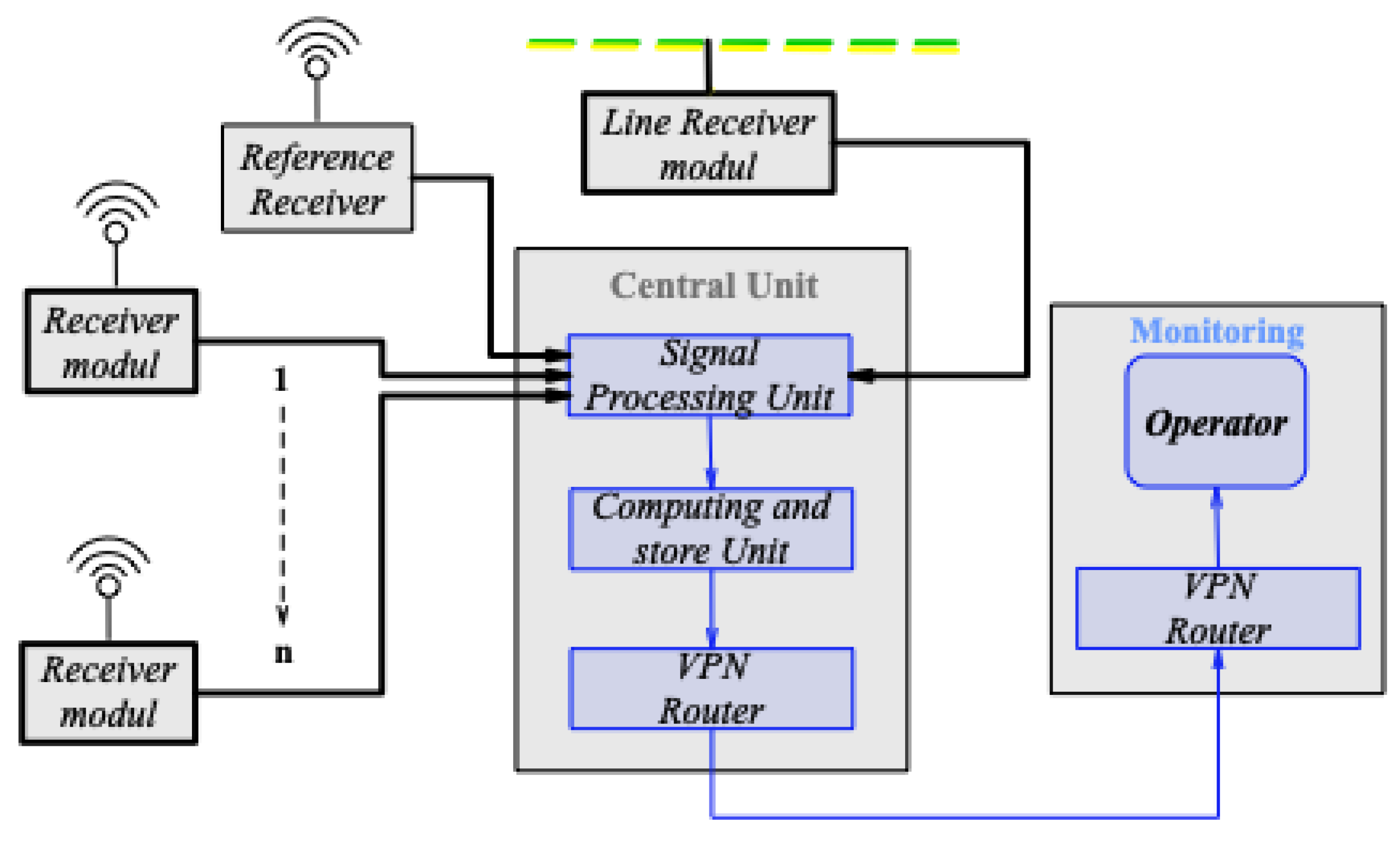
Figure 2.
Step by step approach of the monitoring concept showing the obtained parameters and their analytical contribution to the extended framework.
Figure 2.
Step by step approach of the monitoring concept showing the obtained parameters and their analytical contribution to the extended framework.
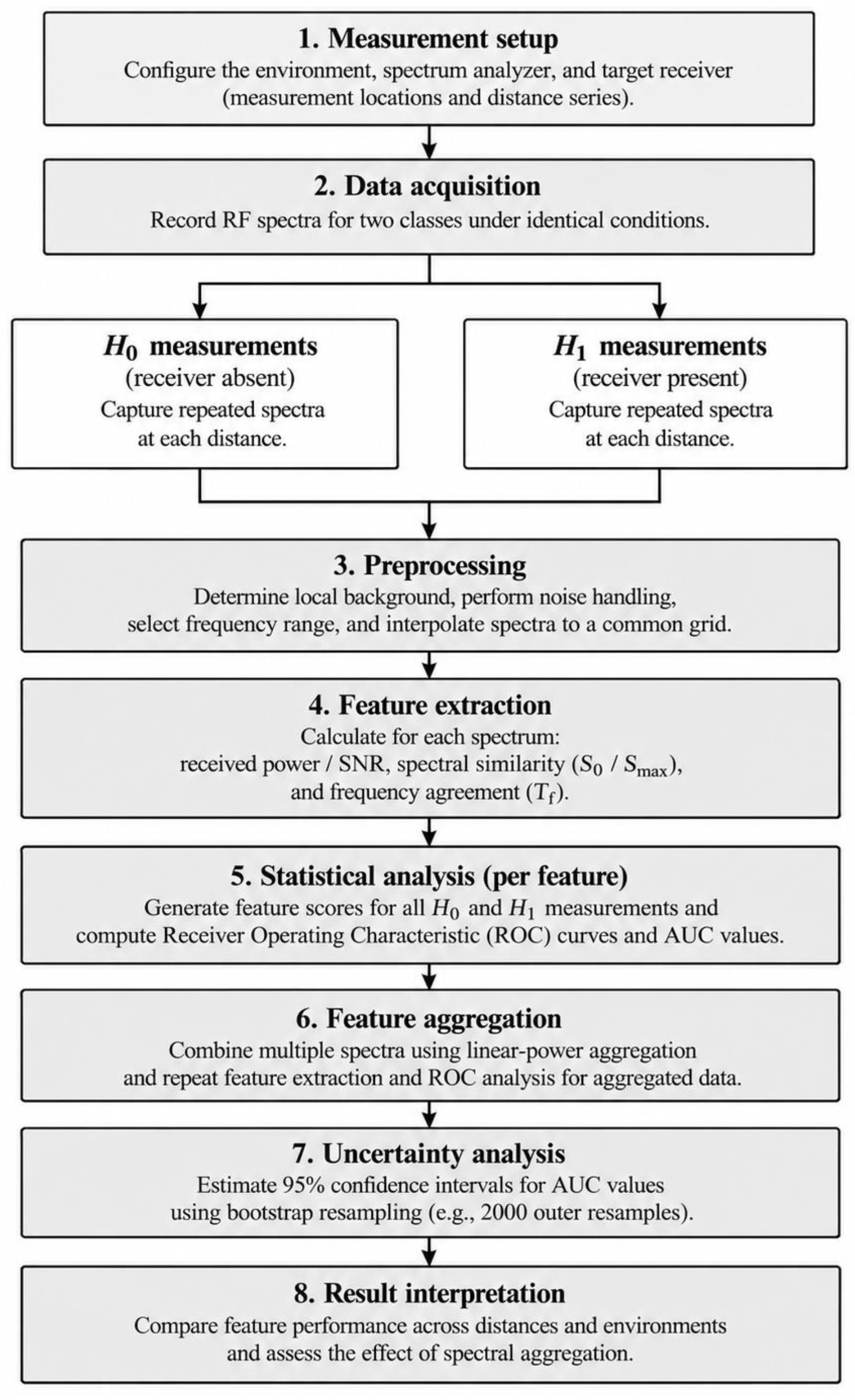
Figure 3.
Near-field characterization of the tested superheterodyne receiver module: (a) H-field probe position used during localization of the receiver-related unintended emission; (b) measured spectral response showing the component in the vicinity of 423.26 MHz.
Figure 3.
Near-field characterization of the tested superheterodyne receiver module: (a) H-field probe position used during localization of the receiver-related unintended emission; (b) measured spectral response showing the component in the vicinity of 423.26 MHz.
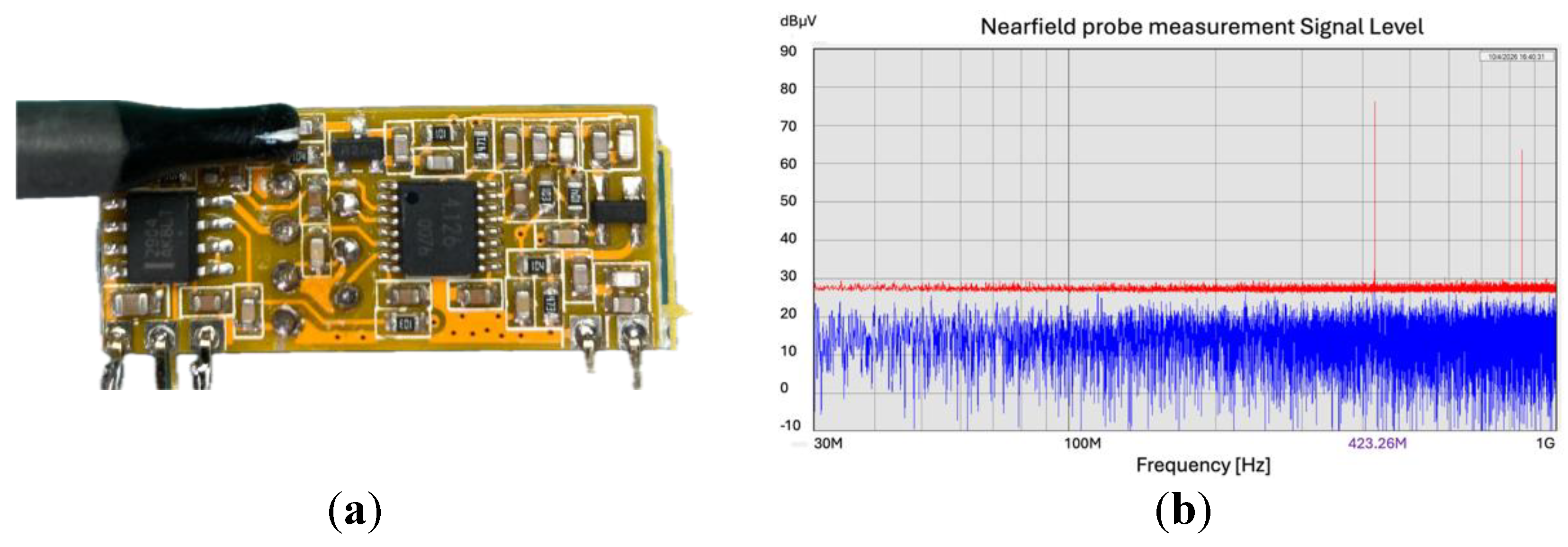
Figure 4.
Simulated indoor propagation conditions for the furnished office measurement environment. The source marker (e.g. RC-IED) indicates the location used in the propagation model. Colours represent the dBm range from -30 (red) to -120 (white) as shown in the bottom-right of the Figure. The four antennas represent the receivers.
Figure 4.
Simulated indoor propagation conditions for the furnished office measurement environment. The source marker (e.g. RC-IED) indicates the location used in the propagation model. Colours represent the dBm range from -30 (red) to -120 (white) as shown in the bottom-right of the Figure. The four antennas represent the receivers.
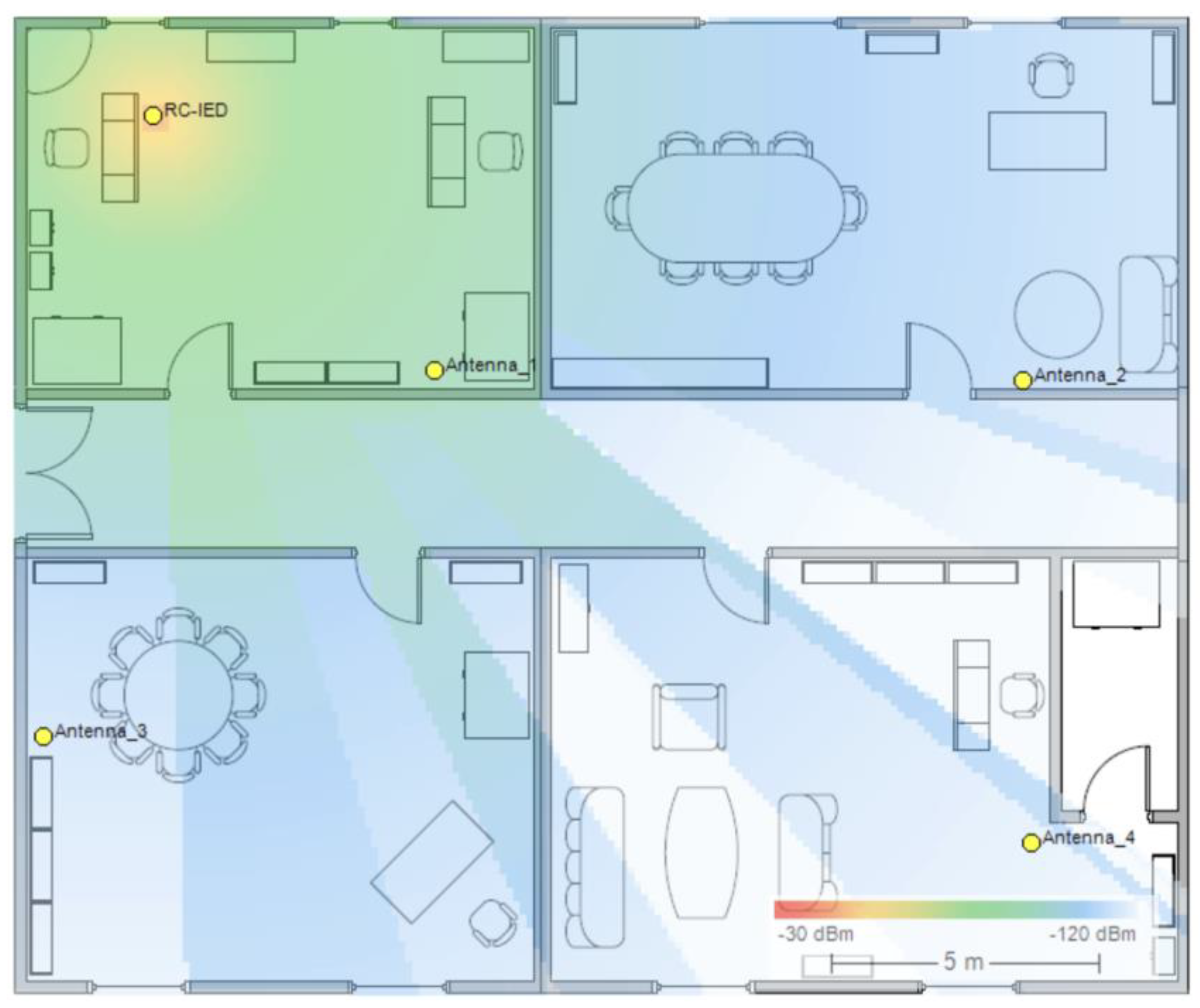
Figure 5.
Log-distance path-loss curves for different values of the path-loss exponent n, illustrating the effect of the assumed indoor propagation environment on distance-dependent attenuation. The curves were generated by MATLAB using formula (2) from the furnished office simulation data (Figure 3).
Figure 5.
Log-distance path-loss curves for different values of the path-loss exponent n, illustrating the effect of the assumed indoor propagation environment on distance-dependent attenuation. The curves were generated by MATLAB using formula (2) from the furnished office simulation data (Figure 3).
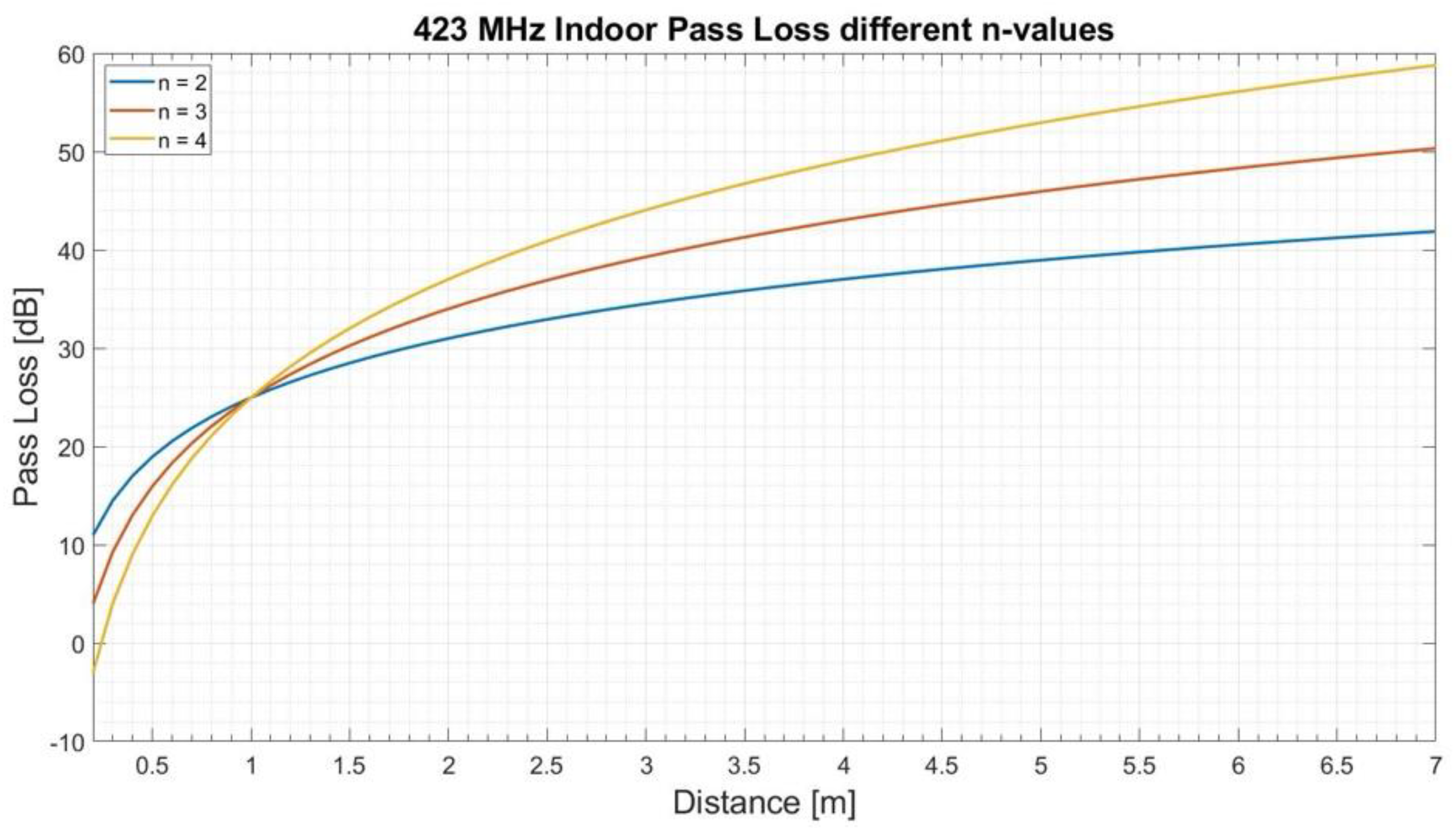
Figure 6.
Measured signal level (magnitude) of the receiver-related component around 423.26 MHz as a function of source-to-sensor distance in the furnished office environment. The frequency range of 410-435 MHz represents the local spectral background including the target frequency of 423.26 MHz. The overall reduction with distance is accompanied by local variations associated with the indoor propagation environment. Magnitude [dBm] is presented in the range of -110 (blue) to -65 (yellow).
Figure 6.
Measured signal level (magnitude) of the receiver-related component around 423.26 MHz as a function of source-to-sensor distance in the furnished office environment. The frequency range of 410-435 MHz represents the local spectral background including the target frequency of 423.26 MHz. The overall reduction with distance is accompanied by local variations associated with the indoor propagation environment. Magnitude [dBm] is presented in the range of -110 (blue) to -65 (yellow).
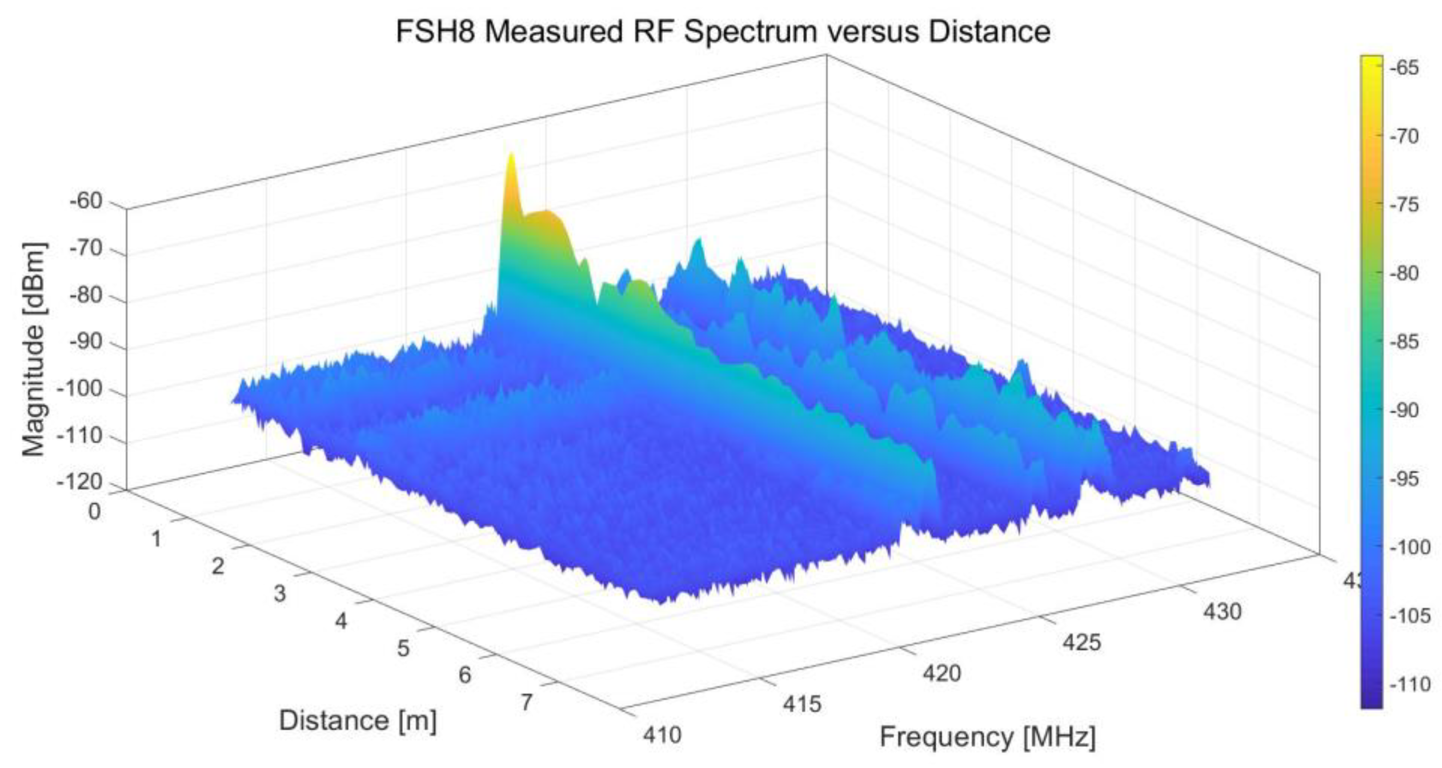
Figure 7.
Distance-dependent evolution of the receiver-related component in the office environment: (a) measured spectral distribution as a function of source-to-sensor distance; (b) target-component level and local SNR calculated relative to the median-based local spectral-background estimate. Coloured lines represent the change in magnitude in dBm (blue) and SNR in dB (red) as a function of distance.
Figure 7.
Distance-dependent evolution of the receiver-related component in the office environment: (a) measured spectral distribution as a function of source-to-sensor distance; (b) target-component level and local SNR calculated relative to the median-based local spectral-background estimate. Coloured lines represent the change in magnitude in dBm (blue) and SNR in dB (red) as a function of distance.
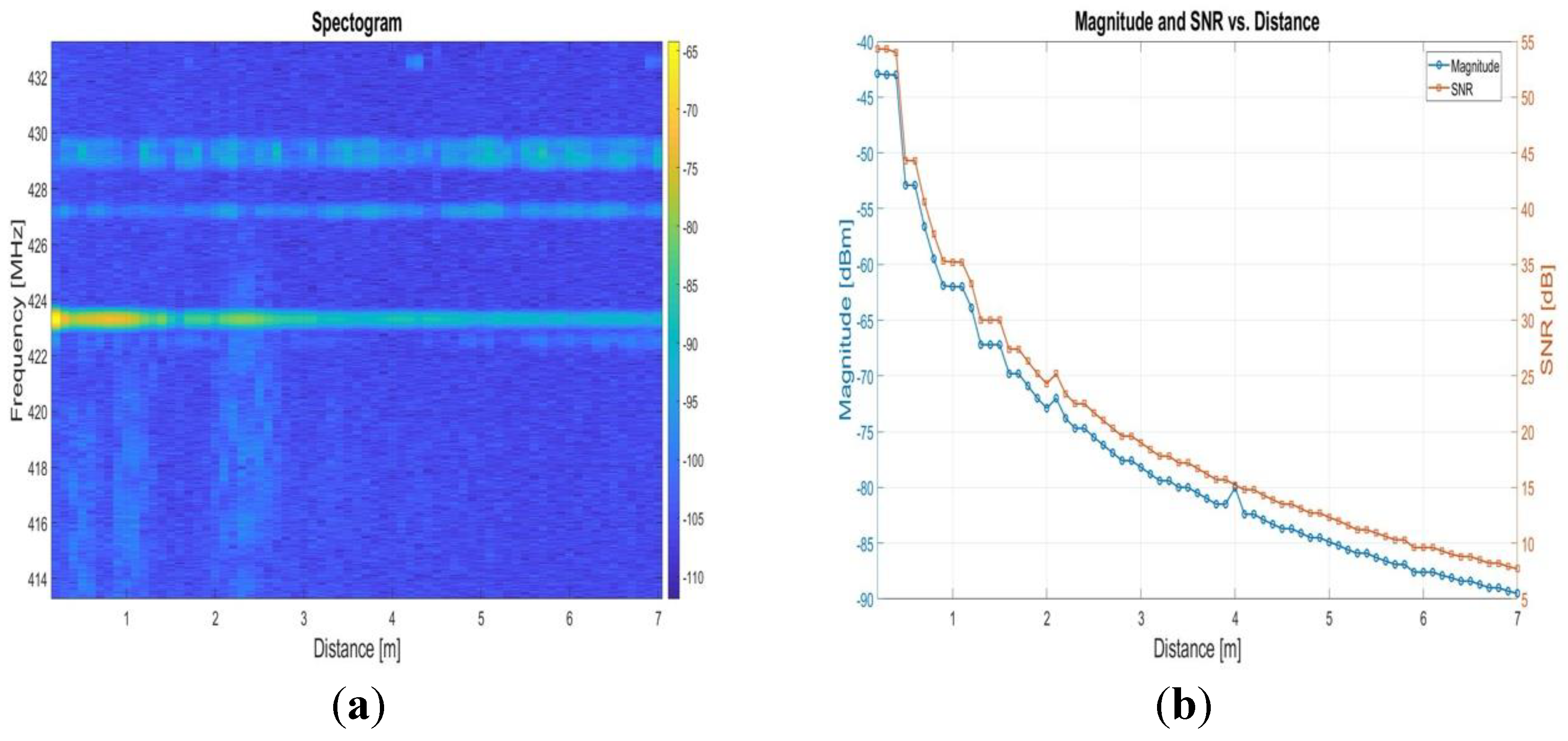
Figure 8.
Measurement of the receiver-related spectral component in the underground environment at source-to-sensor distances extending to 20 m. The comparatively low external RF activity and different propagation conditions provide a complementary measurement configuration to the furnished office environment. Signal level [dBm] is presented in the range of -125 (blue) to -75 (yellow).
Figure 8.
Measurement of the receiver-related spectral component in the underground environment at source-to-sensor distances extending to 20 m. The comparatively low external RF activity and different propagation conditions provide a complementary measurement configuration to the furnished office environment. Signal level [dBm] is presented in the range of -125 (blue) to -75 (yellow).
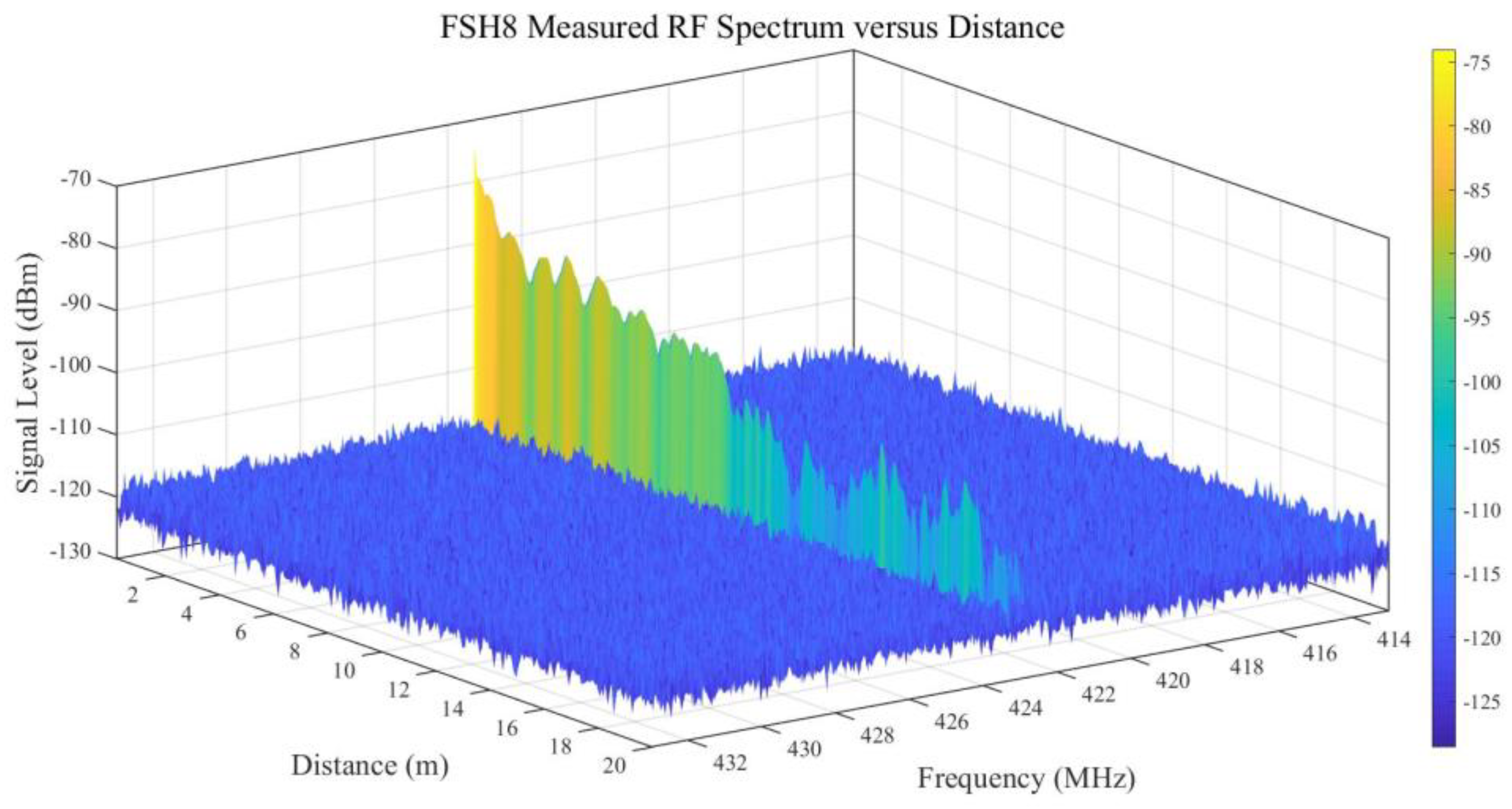
Figure 9.
ROC analysis of the extracted RF features for the receiver-absent (H0) and receiver-present (H1) measurements at 3 m. Target-band peak level and local SNR yielded an AUC of 1.000, the target-frequency-agreement score Tf yielded an AUC of 0.920, while S0 and raw Smax yielded AUC values of 0.560 and 0.348, respectively. The dashed diagonal indicates chance-level discrimination. Smax is shown using its original score orientation.
Figure 9.
ROC analysis of the extracted RF features for the receiver-absent (H0) and receiver-present (H1) measurements at 3 m. Target-band peak level and local SNR yielded an AUC of 1.000, the target-frequency-agreement score Tf yielded an AUC of 0.920, while S0 and raw Smax yielded AUC values of 0.560 and 0.348, respectively. The dashed diagonal indicates chance-level discrimination. Smax is shown using its original score orientation.
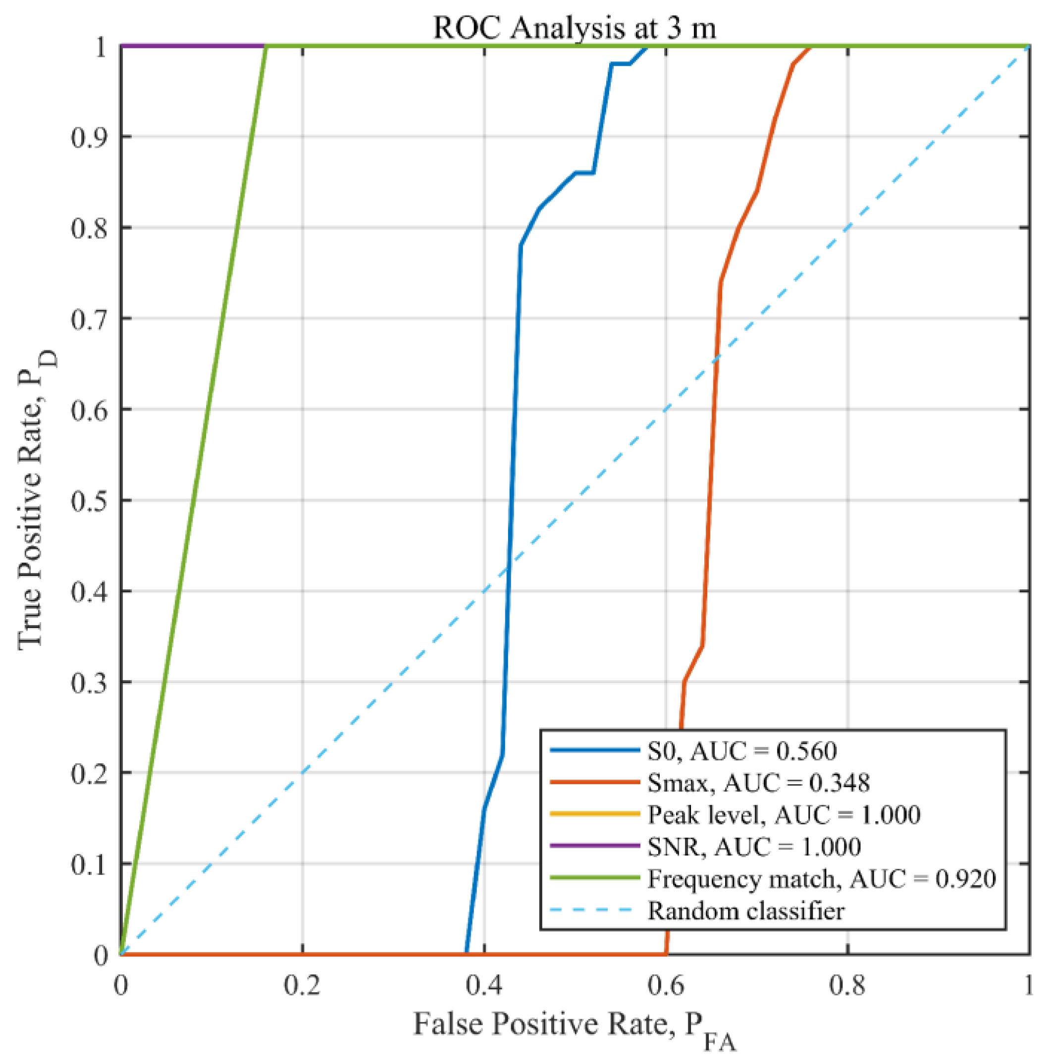
Figure 10.
Direction-oriented AUC of the Sma ,raw feature as a function of the number of aggregated spectra for the 3 (blue line), 5 (red line), and 7 m (yellow line) measurement configurations. Error bars represent 95% percentile bootstrap confidence intervals. The horizontal dashed line represents no change relative to the single-spectrum condition.
Figure 10.
Direction-oriented AUC of the Sma ,raw feature as a function of the number of aggregated spectra for the 3 (blue line), 5 (red line), and 7 m (yellow line) measurement configurations. Error bars represent 95% percentile bootstrap confidence intervals. The horizontal dashed line represents no change relative to the single-spectrum condition.
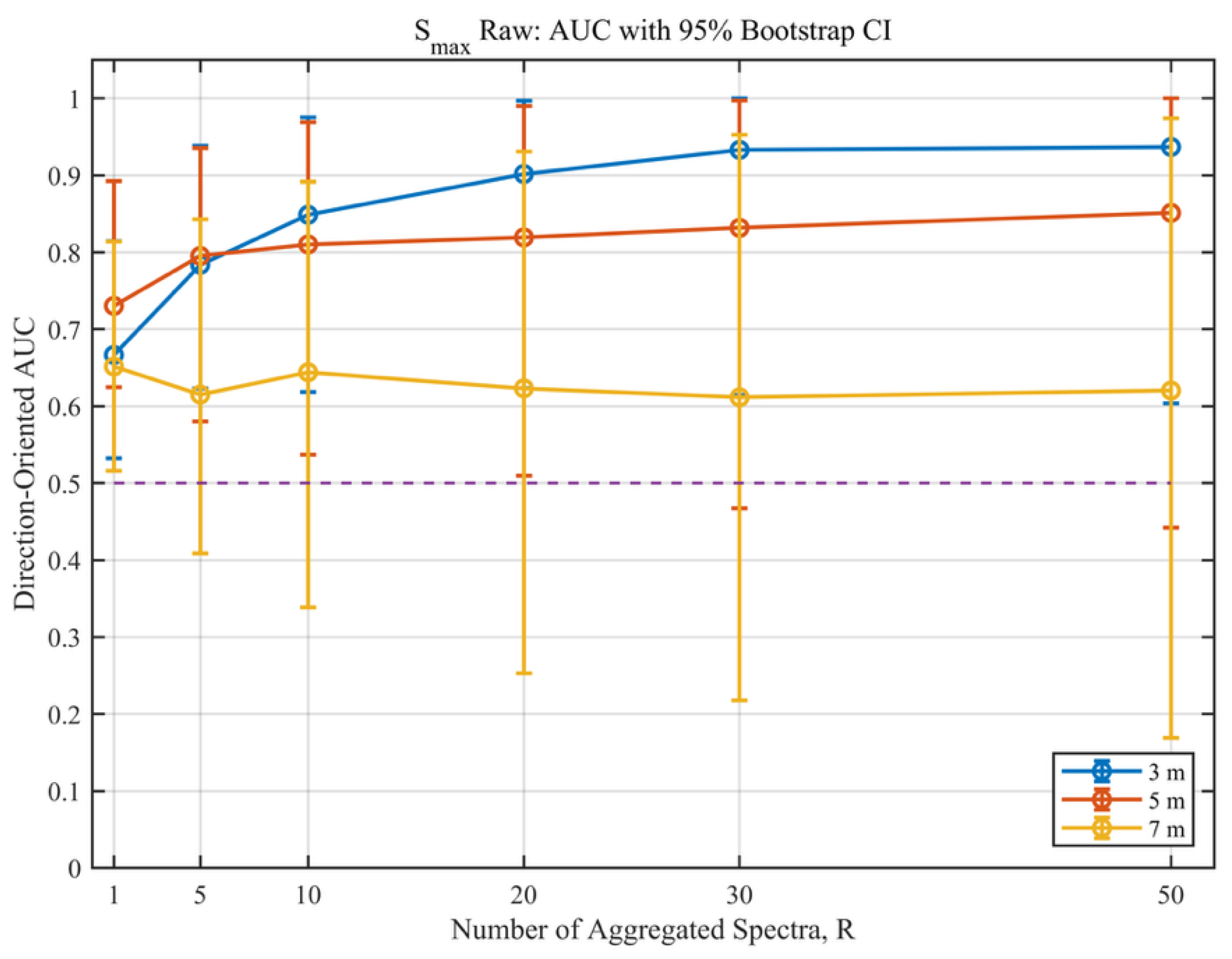
Figure 11.
Paired aggregation gain, ΔAUC(R) = AUC(R) − AUC(1), for the Sma ,raw feature with 95% percentile bootstrap confidence intervals for the three configurations: 3 (blue line), 5 (red line), and 7 m (yellow line) The horizontal dashed line represents no change relative to the single-spectrum condition.
Figure 11.
Paired aggregation gain, ΔAUC(R) = AUC(R) − AUC(1), for the Sma ,raw feature with 95% percentile bootstrap confidence intervals for the three configurations: 3 (blue line), 5 (red line), and 7 m (yellow line) The horizontal dashed line represents no change relative to the single-spectrum condition.
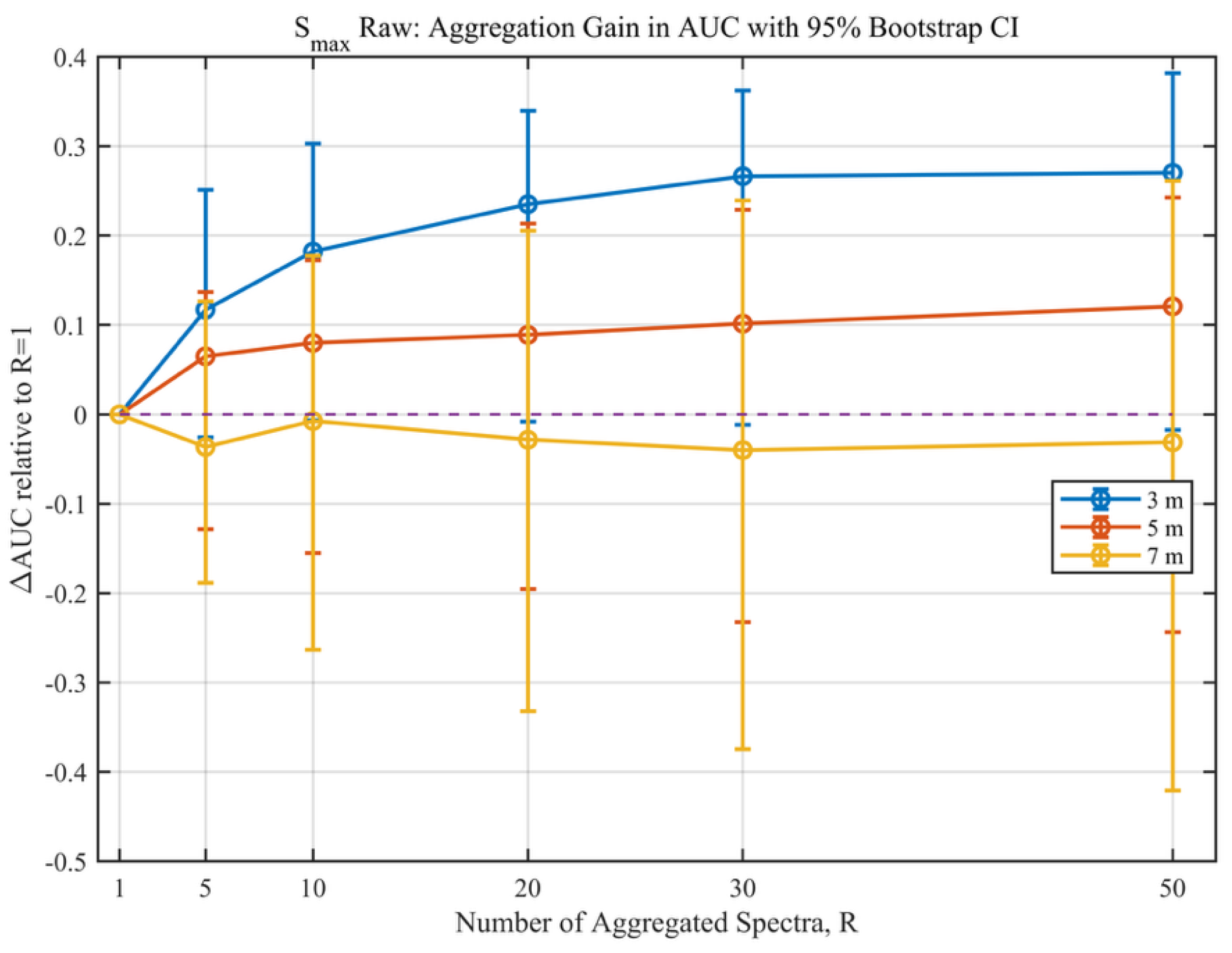

Table 1.
Single-spectrum ROC AUC values of the extracted RF features for the investigated source-to-sensor configurations. The Smax values are reported using the original score orientation; AUC values below 0.5 therefore indicate inverse H0/H1 score ordering. AUC 1.000 corresponds to complete ranking separation of the measured H0/H1 samples.
Table 1.
Single-spectrum ROC AUC values of the extracted RF features for the investigated source-to-sensor configurations. The Smax values are reported using the original score orientation; AUC values below 0.5 therefore indicate inverse H0/H1 score ordering. AUC 1.000 corresponds to complete ranking separation of the measured H0/H1 samples.
| Feature | 3 m AUC | 5 m AUC | 7 m AUC |
|---|---|---|---|
| Peak spectral level, Ppeak | 1.000 | 1.000 | 1.000 |
| Local SNR | 1.000 | 1.000 | 1.000 |
| Target-frequency agreement, Tf | 0.920 | 0.910 | 0.927 |
| Zero-lag similarity, S0 | 0.560 | 0.570 | 0.550 |
| Maximum lag-tolerant similarity, Smax,raw | 0.348 | 0.261 | 0.360 |
Disclaimer/Publisher’s Note: The statements, opinions and data contained in all publications are solely those of the individual author(s) and contributor(s) and not of MDPI and/or the editor(s). MDPI and/or the editor(s) disclaim responsibility for any injury to people or property resulting from any ideas, methods, instructions or products referred to in the content. |
© 2026 by the authors. Licensee MDPI, Basel, Switzerland. This article is an open access article distributed under the terms and conditions of the Creative Commons Attribution (CC BY) license (http://creativecommons.org/licenses/by/4.0/).
Copyright: This open access article is published under a Creative Commons CC BY 4.0 license, which permit the free download, distribution, and reuse, provided that the author and preprint are cited in any reuse.