

Submitted:
17 October 2026
Posted:
19 October 2026
You are already at the latest version
Abstract
Current theories attribute a decisive role in the formation of extreme events to the meanders formed by jet streams when they slow down. These meanders are thought to foster the de-velopment of persistent atmospheric blocking patterns, impeding the westerly flow that carries mild oceanic air while channeling extremely cold, dense Arctic air toward mid-latitudes. It is as if, once released from the "barrier" holding it back, polar air rapidly flows southward via advection. Here, we propose complementing this intuitive, simplify-ing, and holistic approach. The method relies on both the resonant forcing of tropospheric multifrequency Rossby waves into harmonic modes and a joint analysis of the time lag between geostrophic wind velocity anomalies at the tropopause and geopotential height anomalies at the mid-tropopause. This analysis utilizes cross-wavelet coherence and phase—relative to a common reference—for geostrophic wind velocity and geopotential height within the 8.6–17.1-day and 17.1–34.2-day period bands that govern blocking pro-cesses. By establishing causal links, the study demonstrates the importance of geostrophic wind velocity anomalies—associated with polar vortices and polar jet streams—in the formation of mid-latitude geopotential height anomalies. The findings reveal that the his-toric cold wave striking North America in January and February 2026—resulting from a split in the stratospheric polar vortex—was driven by a vast annular high-pressure system acting as an anticyclone. Similarly, the successive heatwaves experienced by Europe dur-ing the summer of 2026 resulted from coupled eddy systems arising from the interaction between geostrophic winds associated, on the one hand, with a southward-shifted lobe of the tropospheric polar vortex and, on the other, with the displaced polar jet stream.
Keywords:
stratospheric polar vortex
; tropospheric polar vortex
; extreme events
; Northern hemisphere
; wavelet coherence
; wavelet phase
1. Introduction
At mid-latitudes, extreme events in the Northern Hemisphere are most often associated with a disruption of the polar vortices. In winter, a disrupted vortex allows polar air to escape (cold spells). In summer, a disrupted polar system stalls atmospheric dynamics, acting like a “lid” that traps locally generated heat beneath a dome.
1.1. Disruption of Polar Vortices in Winter
Research into the coupling between stratospheric dynamics and extreme surface weather phenomena relies on several major studies that quantify the causal link between the weakening of the polar vortex and the occurrence of cold spells. A pioneering study demonstrates the value of the stratosphere for long-range weather forecasting [1]. The authors statistically demonstrate that the probability of experiencing intense cold spells (cold air outbreaks) in Europe, North Asia, and the East Coast of the United States increases significantly in the 10- to 60-day period following a major weakening of the polar vortex.
Two types of vortex disruption occurring during a Sudden Stratospheric Warming (SSW) event must be distinguished: “displacement” (the vortex shifts off its axis) and “splitting” (the vortex breaks into two distinct vortices) [2]. The study reveals that tropospheric cold waves following a vortex split are significantly more severe, geographically widespread, and long-lasting than those resulting from a simple displacement. Research published following the devastating February 2021 freeze in Texas [3] identifies a specific state of disruption: vortex stretching. The study concludes that sea ice loss in the Barents and Kara Seas increases the frequency of this stretching, which forces the jet stream to plunge deeply toward the southern United States, bringing historic negative temperature anomalies.
Analysis of the polar vortex’s evolution since the late 20th century has shown that periods during which the vortex is weak, stretched, or disrupted have become much more persistent [4]. This prolonged duration of disrupted phases is directly responsible for an increase in extreme cold waves across continental Eurasia, providing a concrete link between climate change and certain local winter cold events.
1.2. Disruption of Polar Vortices in Summer
Although the impact of polar vortices on extreme weather events is primarily a winter phenomenon, strong coupling has recently been identified between spring or summer vortex disruptions (and associated jet stream disturbances) and the occurrence of heatwaves at mid-latitudes. The mechanism involves not the descent of cold air, but the formation of persistent anticyclonic blocking patterns (heat domes) caused by a disrupted, highly meandering jet stream.
A severely disrupted and slowed polar jet stream forms extreme meanders, that is, stationary Rossby waves [5]. The authors demonstrate that this disruption traps powerful anticyclones (heat domes) simultaneously over North America, Europe, and Asia. These “locked” waves explain recurring extreme summer heatwaves, revealing that the undulation of the tropospheric vortex is the primary driver of persistent heat.
Under normal conditions, the stratospheric polar vortex naturally dissipates in the spring during the “Final Stratospheric Warming” event [6]. This paper analyzes how the timing and abruptness of this final breakup influence weather patterns in the following months. An early or particularly intense disruption in the spring alters the North Atlantic Oscillation (NAO) in a lasting way, thereby favoring the establishment of dry, warm anticyclones over Europe in early summer, increasing the risk of early-season heatwaves.
With the rapid warming of the Arctic (ice melt), the temperature difference between the pole and the equator is decreasing [7]. The study explains that this significantly weakens polar atmospheric circulation (the jet stream). Instead of rapidly sweeping weather systems along, high-altitude winds stagnate. This slowdown prevents low-pressure systems from advancing and traps masses of warm air over Europe and Russia, causing intense and deadly heatwaves.
A study examines the influence of the Antarctic polar vortex on an extreme event that occurred in Australia. The extreme disruption resulting from a SSW of the Antarctic polar vortex in late 2019 led to a historic event [8]. The study demonstrates that the breakdown of this vortex caused a shift in westerly winds toward the equator, drastically drying out Australia. This coupling was the direct meteorological trigger for the record-breaking heatwaves and the infamous Australian “Black Summer” (megafires) of 2019–2020.
1.3. Current Theories Rely on an Intuitive, Simplifying, and Holistic Approach
Current theories attribute a decisive role to the meanders formed by jet streams as they slow down. These meanders in the jet stream are thought to foster the development of persistent atmospheric blocking patterns (such as high-pressure systems stalled over the Atlantic, Greenland, or Scandinavia). These configurations obstruct the usual westerly flow that brings mild oceanic air. They act as “funnels” or corridors that literally draw in extremely cold, dense Arctic air, channeling it directly toward mid-latitudes (North America, Europe, or Asia); this means that, once released from the “barrier” that had held it back, the polar air flows rapidly southward via advection.
1.4. A New Methodological Approach
Joint wavelet analysis—conducted within specific period ranges—of geostrophic wind velocities at the tropopause and geopotential height at the mid-tropopause reveals causal relationships. These relationships highlight specific mechanisms leading to the formation of blocked vortex systems. This approach relies on the ability of multi-frequency Rossby waves to be resonantly forced into harmonic modes at the tropopause, which arises from general considerations relating to the collective behavior of these waves. Multi-frequency Rossby waves are considered as coupled inertial oscillators governed by the Caldirola–Kanai (CK) equations [11,12]. These equations express a boundary condition that the geostrophic wind velocities and must satisfy when the geostrophic balance of the dynamical system is reached. This boundary condition is expressed by the restoring force of the various coupled oscillators. The restoring forces between the different waves are all the stronger when the imbalance between the Coriolis force and the horizontal pressure gradients is significant. However, the geostrophic balance is not disrupted when .
Since the period of the fundamental wave coincides with the forcing period, harmonics occur, the periods of which are multiples or divisors of the fundamental wave’s period. This condition is necessary to ensure the stability of the dynamic system formed by the superposition of coupled multifrequency quasi-stationary waves. When these conditions are met, each oscillator receives, on average, as much energy from the other oscillators as it releases.
Rossby waves result from the variations in height of the interface at the tropopause of polar vortex, polar or subtropical jet streams. These interfaces move up-and-down de-pending on whether the column of air supporting them is warm or cold (polar and sub-tropical waves are in opposite phase), which generates zonal and meridional geostrophic winds.
In all cases, the fundamental wave undergoes a heating followed by a cooling during each period (one year here). This alternation results from the variation in solar irradiance. Oscillations of the interface of the fundamental wave produce harmonics whose oscillations similarly reflect a heating followed by a cooling during each period. Geostrophic winds are warm when blowing in one direction and cold when blowing in the other; depending on the period, this can induce geopotential height anomalies (GHAs) associated with blocking phenomena.
1.5. The Aim of this Study
The present study focuses on the thermodynamic properties of the geostrophic winds associated with jet streams. These geostrophic winds, resulting from Rossby waves, enter into resonance under the influence of the sun’s declination. By focusing on period bands corresponding to various harmonic modes of Rossby waves, causal relationships are established between geostrophic wind velocity anomalies (GWVAs)—associated with polar vortices as well as polar jet streams—and geopotential height perturbations. The purpose of this new approach is to offer fresh insight into the mechanisms leading to extreme events during polar vortex disruptions, using as case studies the historically cold period that affected North America in the winter of 2026 and the historically warm period that affected Europe during the summer of that same year.
2. Materials and Methods
2.1. Data
All data are provided by Copernicus Climate Change Service, Climate Data Store, (2024): ERA5 post-processed daily-statistics on pressure levels from 1940 to present, (0.25° × 0.25°) resolution. Copernicus Climate Change Service (C3S) Climate Data Store (CDS), DOI: 10.24381/cds.50314f4c (Accessed on 09-October-2026) [9], that is, the zonal and meridional wind velocities and at 50 hPa and 250 hPa from which is deduced the absolute velocity , the vertical wind vorticity at 500 hPa, and the geopotential height at 500 hPa.
2.2. Decomposition in Harmonic Modes and Cross-Wavelet Analysis
The spatial and temporal representation of the data—geostrophic wind velocities, geopotential height, and surface temperature—is carried out across period ranges corresponding to harmonic modes. Cross-wavelet analysis of spatially distributed oscillatory phenomena makes it possible not only to express the amplitude (the square root of the wavelet power) of the oscillations but also to establish plausible causal links between distant oscillations within predefined period ranges. Two quantities are essential in this regard: coherence and phase. The coherence measures the degree of similarity between the temporal behavior of two observed oscillations, regardless of any time lag. The phase determines the time lag between the observed oscillations. Depending on the case, the phase is displayed where either the amplitude or the coherence is significant, depending on what needs to be highlighted for the interpretation of the observed phenomena.
The degree of temporal coherence of regionalized variables is expressed relative to a time reference, either the same variable at a specific location or any other state variable. The polar vortex disruption is illustrated in Figure 1, which shows the evolution of the 1/16 year-period harmonic of the stratospheric and tropospheric geostrophic wind velocities at the 50 hPa and 250 hPa levels over the time window centered on January 30, 2026, that is, from January 18, 2026, to February 11, 2026. Indeed, the period range used to represent the 1/16 year-period harmonic, whose average period =22.8 days, is 17.1 to 34.2 days. These two limits correspond to and in order to investigate different harmonic period ranges by applying a scale factor of 2.
GWVAs are characterized by their amplitude, as well as by their coherence and phase relative to the wind velocity at the 50 hPa level (at 75.625° N, 60.625° W), which serves as the temporal reference. This location above far west Greenland is chosen so that the reference can be used as a clock. Indeed, its Fourier transform highlights the two main harmonics with periods 1/16 years and 1/8 years, which can be considered as stable pulsations over time, with a bandwidth that can be considered a signature of the vortex (Figure 2). The phase - displayed only where coherence is high - indicates the time lag between the moments when wind velocity at the reference point and at each regionalized point reach their respective maxima (a single maximum/minimum within a period). In particular, the phase allows distinguishing the geostrophic wind of the subtropical jet-stream at the top of the descending air column shared by the Hadley and Ferrel cells, in opposite phase with the geostrophic wind of the polar jet-stream at the top of the ascending air column shared by the Ferrel and polar cells. In this way, when the reference represents the polar vortex, its phase appears in pink-red—just like that of the subtropical jet geostrophic wind—whereas the phase of the polar jet geostrophic wind appears in dark blue.
On the other hand, coherence highlights causal relationships between the velocity of the stratospheric polar vortex and the regionalized variables, velocity of the geostrophic wind at various altitudes, height of the geopotential at mid-tropopause, and surface temperature. Indeed, the band of periods is wide enough to be able to invoke a causal relationship when the coherence is close to 1 over extended region, exhibiting both temporal and spatial coherence.
3. Results and Discussion
3.1. The Arctic Cold Snap of Winter 2026
The Arctic cold snap of January-February 2026 was caused by a major disruption of the polar vortex, which brought intense cold to North America and Europe [10]. Here, we aim at refining the different mechanisms involved in the formation of the historic cold wave which extended to the south of the United States. This is done by highlighting disruptions to the polar vortices, as well as the chain of induced events which led to this cold spell.
The splitting process of the stratospheric polar vortex is highlighted in Figure 1a-c. The amplitude reveals two poles on either side of the pole—one in the Indo-Asian sector and the other in the North American sector—as typically occurs during the splitting of the stratospheric vortex. Coherence highlights a multitude of fragments whose phase is predominantly pink, with the exception of the Indo-Pacific lobe—flanked by two out-of-phase vortices (in blue) signaling the development of the polar jet—and the North American vortex, bordered by a yellow-orange fringe that is in phase with the tropospheric vortex drifting to the south over Canada (Figure 1d-f).
According to Figure 1c, the subtropical geostrophic wind near 30°N is relatively undisturbed, while undergoing a phase shift—transitioning from pink to blue—over the Atlantic off the coast of West Africa and over the Pacific off the coast of North America, thereby becoming in phase opposition with the polar vortex. At the tropopause, geostrophic winds are highly disturbed. In particular, as shown in the Figure 3c, the southward shift of the polar vortex over Canada, which brings it closer to the polar jet stream 45°N (blue phase), favors the formation of an annular GHA over the North America, creating a dipole (red-orange and light-blue phases) as shown in Figure 3f.
Selecting a common reference for both GWCAs and GHAs makes it possible to establish a link between them because of their high coherence (Figure 3b, e); indeed, the interactions between geostrophic wind velocity variations and the geopotential height response being brief compared to the period band, they can be considered instantaneous. The phase relationship between GWVAs and the geopotential height response is established based on the color association. Their synchrony arises from the fact that any positive GWVA (warm wind directed eastward) corresponds to a positive GHA (high-pressure system). Conversely, any negative GWVA (cold wind directed westward) corresponds to a negative GHA (low-pressure system). Any GHA can be associated with a GWVA between latitudes 40°N and 70°N.
The shifted geostrophic jet polar wind—whose maximum eastward velocity is reached on February 3, 2026, four days after the geostrophic wind of the time reference peaked on January 30, 2026—induces a giant vortex above the North and Central America, as revealed in Figure 3b, c by the coherence and phase of the 500 hPa geopotential height. Resulting from the combined action of the geostrophic wind of the tropospheric polar vortex and the polar jet, in opposite phase, this giant vortex forms an out-of-phase dipole, oscillating between a reddish-orange phase and a light-blue phase in its southeastern section. It behaves alternatively like an anticyclone as is the case during the half-period from January 22, 2026, to February 15, 2026 (maximum eastward velocity reached on February 3, 2026, in its northern part), and like a cyclonic system. Its existence is closely linked to the behavior of the stratospheric polar vortex via the shifted tropospheric polar vortex, as demonstrated by the strong coherence of both the tropospheric polar vortex and the GHA (Figure 3b, e).
Figure 4c, d show the surface air temperature anomalies observed over a period extending from January 18, 2026, to February 11, 2026. The association between the color patterns of the phase of both the surface temperature anomalies and GHAs are highlighted at latitudes north of 30°N (Figure 4b, d).
The Figure 4d shows two surface temperature anomalies in phase opposition. This dipole consists of an anomaly located at high latitudes concomitant with the polar vortex (blue phase meaning that the temperature anomaly is positive on January 30, 2026), and an anomaly between latitudes 30°N and 60°N concomitant with the giant annular GHA (red phase meaning that the temperature anomaly is negative on January 30, 2026). Only the outline of the negative temperature anomaly is the result of the anticyclonic system active between January 24, 2026, and February 5, 2026 (the system becomes cyclonic outside this time window—specifically, from January 18 to 23, 2026, and from February 6 to 11, 2026).
However, the boundaries of the zone of low coherence—located at the center of the vast anticyclonic system (Figure 4e, f)—coincide with the temperature anomaly (Figure 4c, d). This coincidence highlights the mechanism that led to the formation of the cold anomaly, which results from cold air descending from the tropopause. This mechanism is decoupled from the stratospheric polar vortex because it reflects the dynamics of the anticyclone, which tends to smooth out temporal variations in the downward air movement while adding noise to it. At the center of the anticyclonic system, a cold-air subsidence effect occurs (blue phase), as shown in the Figure 4g, h: the velocity of the descending air is on the order of 0.20 m/s, covering a broad area that encompasses central North America.
In summary, considering the 17.1–34.2-day period band, the combination of GWVAs—linked, on one hand, to a lobe of the tropospheric polar vortex shifted over Canada, and on the other, to the polar jet at 45°N over North America (in phase opposition)—led to the formation of a giant anticyclonic annular system. The cold wave over North America resulted from this high-pressure system, which persisted for half a period.
3.2. The Arctic Heatwave of Summer 2026
3.2.1. Geostrophic Wind Velocities at the 250 hPa Level in the 17.1-34.2-Day Period Band
Based on the Figure 5, the amplitude and phase of geostrophic wind velocities at the Northern Hemisphere tropopause—represented within the 17.1–34.2 and 8.6–17.1 day period bands—reveal a disrupted tropospheric polar vortex (pink or orange-yellow phase) split in two on either side of the pole (Figure 5b). These synchronous polar vortices are surrounded by the polar jet stream—whose geostrophic wind phase is depicted in blue—which is itself surrounded by the subtropical geostrophic wind (orange-yellow phase). Thus, the geostrophic winds of the tropospheric polar vortex, the polar jet stream, and the subtropical jet stream are alternately in opposite phase.
Figure 6 shows the sequence of anomalies in the 17.1–34.2-day period band—corresponding to the 1/16-year period harmonic—for the geostrophic wind velocity at the 250 hPa level and the geopotential height at the 500 hPa level. The first column represents the amplitude of the anomalies (square root of the wavelet power). The reference time series used in the cross-wavelet coherence (second column) and phase (third column) is the 500 hPa geostrophic wind velocity at 70°N, 10°E for all anomalies. Selecting this reference point—relative to the southward-shifted vortex located between Western Europe and Greenland—causes the latter’s phase to appear in pinkish-red hues, as it is close to zero by design. This makes it possible to distinguish the southward-shifted vortex from the geostrophic winds of the main vortex (when it is still visible) and of the polar jet stream, which is in phase opposition (shown in blue).
The observation dates indicated in the Figure 6 correspond to the successive maxima of the reference time series within this period band. In this way, the successive observation periods comprehensively cover the timeframe extending from May 16, 2026, to August 22, 2026. The phase is displayed where the GWVA exceeds 6 m/s or where the GHA exceeds 41 m (400 gpm).
Here again, the temporal reference plays a dual role. On the one hand, it indicates the chronology of events, enabling them to be linked. On the other, it establishes a causal connection where coherence is high, whether concerning GWVAs or GHAs. In this instance, the southward shifted polar vortex’s contribution to the observed anomalies over Europe and northwestern Asia is confirmed.
Regarding the observation date of May 28, 2026 (Figure 6a-f), the main polar vortex (blue phase) is the driver of the GHA affecting both Europe and northwestern Asia. Geopotential height peaks four days prior to the observation date (blue phase as well), specifically on May 24, 2026, revealing two giant high-pressure systems originating from the variations in the main polar vortex velocity, and exhibiting high horseshoe-like coherence (Figure 6e); these systems are separated by a narrow high-pressure system originating from the vortex that detached from the main vortex and is in phase opposition to it (red phase). They are generating two anticyclonic systems centered over northwestern and northeastern Europe (Figure 6e), giving rise to two heat domes (Figure 7a, b): one centered over France—peaking between May 26, 2026 (indigo phase) and May 28, 2026 (pink phase) as it moves from west to east across the country—and the other located over northwestern Russia, peaking on May 24, 2026 (blue phase).
Regarding the observation date of June 23, 2026 (Figure 6g-l), the key role of polar vortices in GHAs west of 40°E is particularly highlighted by the correspondence between the GWVA and the GHA at 20°E (red phase). However, the low coherence of both anomalies (Figure 6h, k) indicates that the southward shifted polar vortex—having detached from the main vortex—becomes independent. A phase continuum is observed both along the GWVAs and along the GHAs, shifting from red to blue in a westward direction; this reveals the progression of the waves from the primary vortex to the secondary vortex over the course of half a period (approximately ten days). However, east of 40°E, the correspondence is established between the GWVA formed by the geostrophic wind of the polar jet (blue phase) and the 60°E GHA. Under the influence of the high-pressure system, a heat dome develops south of the GHA and concomitantly with it, centered primarily over France (Figure 6j-l and Figure 7c, d).
The anomalies observed on July 18, 2026, are again divided between those influenced by the polar vortices west of 40°E and those governed by the geostrophic component of the polar jet east of 40°E. In this case, only the southward-displaced polar vortex is involved, as it undergoes splitting—suggested by the phase change occurring along a zonal band further south (green-yellow-orange phase) (Figure 6m-r). As for the polar jet, it exhibits a more stable geostrophic wind at the tropopause, establishing a pseudo-continuity on either side of 20°E. The heat dome that was situated over Western Europe is dissipating, giving way to two anticyclonic systems—located at 20°W and 20°E—that are driving warm, dry winds across the region. This creates a significant disparity between the temperature anomaly over France and the one further east, nearly in opposite phase (Figure 7e, f).
On August 11, 2026, the southward shifted geostrophic wind at the tropopause is once again disrupted by the splitting of a secondary southward shifted polar vortex, pushing the polar jet’s geostrophic wind further south (Figure 6s-x). The phase of the two high-pressure systems east of 40°E reverses, forming a cyclone-anticyclone dipole. The temperature anomalies observed over Western Europe subside, dropping below 1 °C, whereas they reached 5 °C at the end of May (Figure 7g, h).
In summary, the disruption of the polar vortex during the observation period severely impacted the climate of Europe west of 40°E within the 17.1–34.2-day period range. Western Europe was particularly affected, experiencing significant economic and societal consequences due to the intensity and duration of heat spikes—with the blocking pattern reflecting the long 22.8-day period (a 1/16-year period harmonic).
3.2.2. Geostrophic Wind Velocities at the 250 hPa Level in the 8.6-17.1-Day Period Band
Another period range reflecting the interactions between geostrophic winds at the tropopause and the geopotential height response—from 8.6 to 17.1 days—represents the 1/32-year-period harmonic. As shown in the Figure 8, the tropospheric polar vortex is highly fragmented, forming a ring centered on the pole with a green-yellow-orange phase. The southernmost lobe is located over northern Europe and northwestern Asia. This ring is encircled by the geostrophic wind of the polar jet, which has a blue phase. Further out, one can distinguish the geostrophic wind of the subtropical jet—with a pink or green-yellow-orange phase—and even the geostrophic wind of the ITCZ over the Atlantic Ocean, recognizable by its blue phase.
The time interval during which the polar vortex exerts a highly significant influence on air temperature extends from mid-May to late June (Figure 9). A high-pressure system extends over Northern Europe (yellow-orange phase) throughout the observation period, from mid-May to early July. This blocking pattern results from the southernmost polar vortex lobe extending east of 20°E (yellow-orange phase). The geostrophic wind pattern, which is difficult to decipher in Figure 9c, becomes easier to interpret in Figure 9i due to the continuity of the polar jet’s geostrophic component (light blue phase) as well as in Figure 9o owing to the visibility of the main polar vortex between 70°N and 80°N (dark blue phase).
The interpretation of the geopotential height response to geostrophic winds is more complex west of 20°E. The complexity of geostrophy is manifested in the multiplicity of polar vortices and the phase mutation (red and light blue) of the geostrophic wind at 20°W (Figure 9o, u). The geostrophic winds involved result in a cluster of GHAs identifiable by their phase, the correspondence being established between GWVAs and GHAs. Unlike the GHA over northeastern Europe, for which coherence can be high (Figure 9j-l), the coherence of the cluster of GHAs over the Atlantic remains very low over the period of observation (Figure 9d-f, j-l, p-r, v-x), indicating that its evolution is decoupled from that of the tropospheric polar vortex.
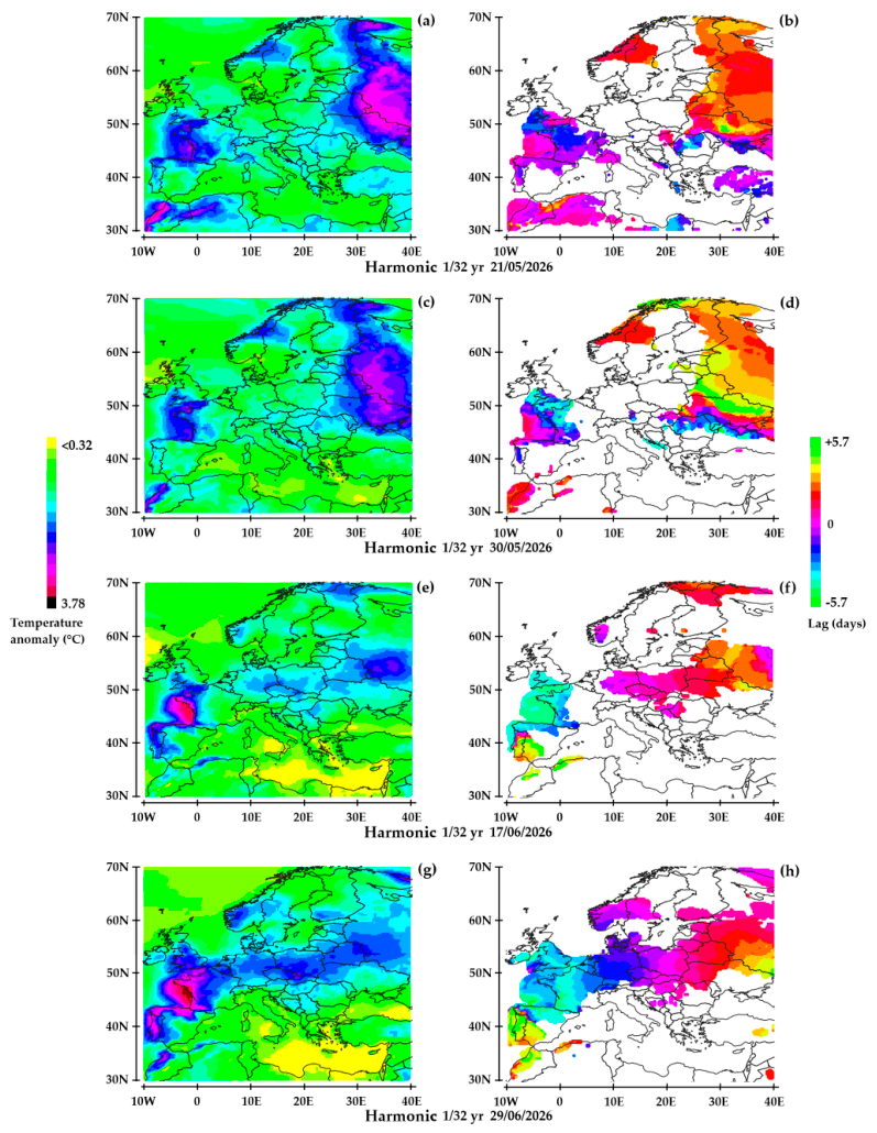
The weather conditions resulting from the remanence of the dipole identified from the cluster of GHAs over the Atlantic west of England and the main GHA over Northern Europe—are highly variable. The Figure 10 highlights an air temperature anomaly between the two poles on June 17, 2026, and June 29, 2026. This indicates that the westernmost pole generates a dominant anticyclonic system that is synchronized with the easternmost anticyclonic system. This results in a warm, dry easterly wind over mid-latitude Europe, causing an anomaly of nearly -4 °C over western France; the heat dome peaks four days prior to the observation dates (light blue phase)—specifically on June 13, 2026, and June 25, 2026. The heatwave takes 7 to 8 days to cross Europe from west to east, with the phase shifting from light blue to reddish-orange. This offset indicates that the phase of the anticyclone over the Atlantic is a few days ahead of that of the anticyclone over Northern Europe. This led to contrasting air temperature anomaly trends between Western and Northeastern Europe: rising in the former and falling in the latter. It follows that it can be inferred that the coupling of the two poles results from the western eddy system being drawn along by the eastern eddy system, such that the former gradually swells at the expense of the latter, which acts as the driver coupled to the polar vortex.
In summary, the disruption of the tropospheric polar vortex contributed to the formation of a dipole of stable eddy systems between mid-May and early July 2026, within the 8.6–17.1-day period range. At the time of observations, the anticyclonic system over northeastern Europe resulted from a warm geostrophic wind from the polar vortex blowing eastward (the wind direction reverses with the sign of the vortex system after half a period). The vortex system over the Atlantic has a more complex origin, involving disturbed geostrophic winds. It benefits from a dragging effect resulting from the coupling of the two poles.
Funding
“This research received no external funding”.
Conflicts of Interest
“The author declare no conflicts of interest.”.
References
- Kolstad, E. W.; Breiteig, T.; Scaife, A. A. The association between stratospheric weak polar vortex events and cold air outbreaks. In Quarterly Journal of the Royal Meteorological Society; 2010. [Google Scholar]
- Mitchell, D. M.; Charlton-Perez, A. J.; Gray, L. J. The Influence of Stratospheric Vortex Displacements and Splits on Surface Climate. J. Clim. 2013. [Google Scholar] [CrossRef]
- Cohen, J.; Agel, L.; Barlow, M.; Garfinkel, C. I.; White, I. Linking Arctic variability and change with extreme winter weather in the United States; Science, 2021. [Google Scholar]
- Kretschmer, M.; Coumou, D.; Agel, L.; Barlow, M.; Tziperman, E.; Cohen, J. More-Persistent Weak Stratospheric Polar Vortex States Linked to Cold Extremes; Bulletin of the American Meteorological Society (BAMS), 2018. [Google Scholar]
- Kornhuber, K.; et al. “Amplified Rossby waves enhance risk of concurrent heatwaves in major breadbasket regions”. Nat. Clim. Change 2020. [Google Scholar] [CrossRef]
- Domeisen, D. I. V.; et al. “The role of the stratosphere in subseasonal to seasonal prediction: Predictability arising from stratosphere-troposphere coupling”. J. Geophys. Res. 2020. [Google Scholar] [CrossRef]
- Coumou, D.; et al. “The influence of Arctic amplification on mid-latitude summer circulation”. In Nature Communications; 2018. [Google Scholar]
- Lim, E.P.; Hendon, H.H.; Boschat, G.; et al. Australian hot and dry extremes induced by weakenings of the stratospheric polar vortex. Nat. Geosci. 2019, 12, 896–901. [Google Scholar] [CrossRef]
- Hersbach, H.; Comyn-Platt, E.; Bell, B.; Berrisford, P.; Biavati, G.; Horányi, A.; Muñoz Sabater, J.; Nicolas, J.; Peubey, C.; Radu, R.; Rozum, I.; Schepers, D.; Simmons, A.; Soci, C.; Dee, D.; Thépaut, J.-N.; Cagnazo, C.; Cucchi, M. ERA5 post-processed daily-statistics on pressure levels from 1940 to present. Copernicus Climate Change Service (C3S) Climate Data Store (CDS). Accessed on. 2023. (accessed on 09-October-2026). [CrossRef]
- Flis, Andrej. A Major Polar Vortex Disruption will bring the Coldest Air of the Season to North America and Cold to Europe. Available online: https://www.severe-weather.eu/global-weather/new-polar-vortex-disruption-forecast-coldest-winter-air-united-states-canada-europe-fa/ (accessed on 13/09/2026).
- Pinault J-L, A Review of the Role of the Oceanic Rossby Waves in Climate Variability. J. Mar. Sci. Eng. 2022, 10(4), 493. [CrossRef]
- Pinault, J.-L. Resonant Forcing by Solar Declination of Rossby Waves at the Tropopause and Implications in Extreme Events, Precipitation, and Heat Waves—Part 1: Theory. Atmosphere 2024, 15, 608. [Google Scholar] [CrossRef]
Figure 1.
Geostrophic wind velocity anomalies at the 50 hPa level (a-c) and at the 250 hPa level (d-f) in the 17.1-34.2 day period band – The first column shows the amplitude (m/s), the second the coherence, and the third the phase (lag) in days. The phase is displayed where the coherence is significant (). The reference is the wind velocity at the 50 hPa level, 75° N, 60° W whose maximum is reached on January 30, 2026.
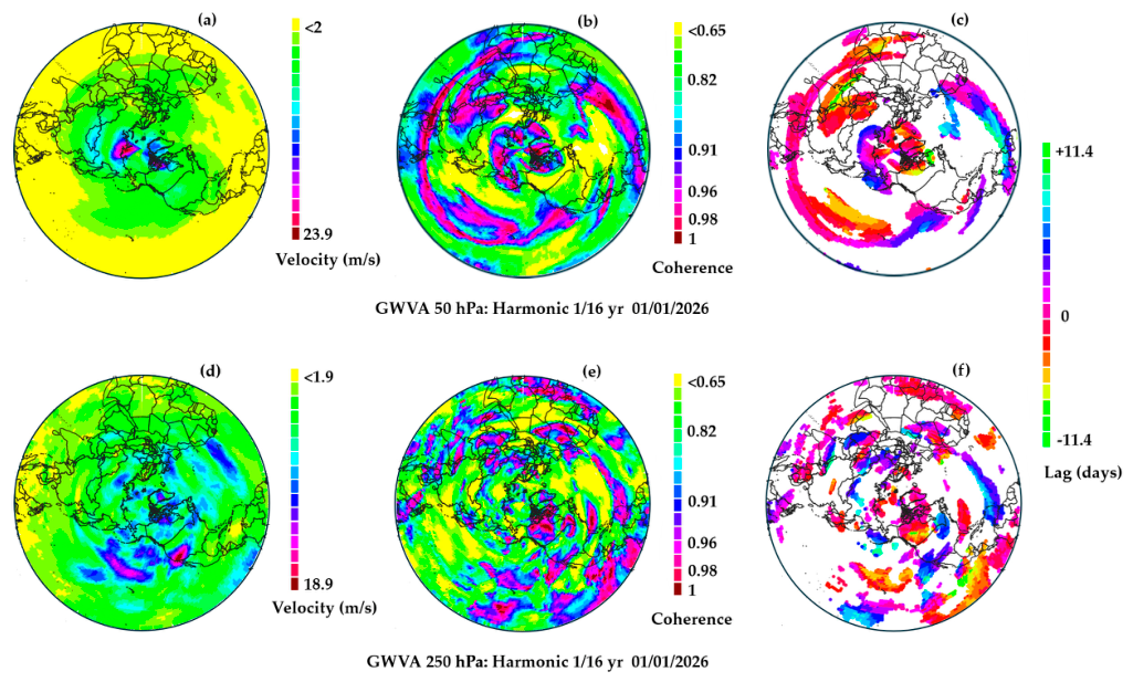
Figure 2.
Fourier spectrum of the wind velocity at 50 hPa (75.625 N; 60.625 W). The two main harmonics, with periods of 22.8 days (i.e., 1/16 of a year) and 45.6 days (i.e., 1/8 of a year), are identified.
Figure 2.
Fourier spectrum of the wind velocity at 50 hPa (75.625 N; 60.625 W). The two main harmonics, with periods of 22.8 days (i.e., 1/16 of a year) and 45.6 days (i.e., 1/8 of a year), are identified.
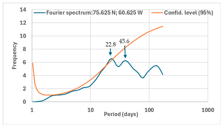
Figure 3.
Geostrophic wind velocity anomalies at the 250hPa level (a-c) and geopotential height anomalies at the 500 hPa level (d-f) in the 17.1-34.2 period band: amplitude in the first column, coherence in the second, phase in the third. The phase is displayed where the coherence is significant (). Same reference as in Figure 1.
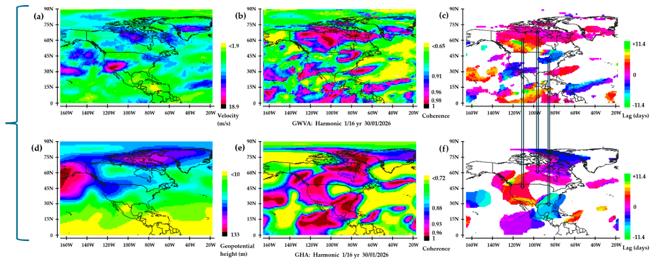
Figure 4.
Within the 17.1-34.2 day period band: Geostrophic wind velocity anomalies at the 250 hPa level (a, b), Air temperature anomalies (c-f), Vertical wind velocity anomalies (g-h). Amplitude (c, g), Coherence (a, e), Phase (b, f) displayed where the coherence is significant (), Phase (d, h) displayed where the amplitude is significant. Same reference as in Figure 1.
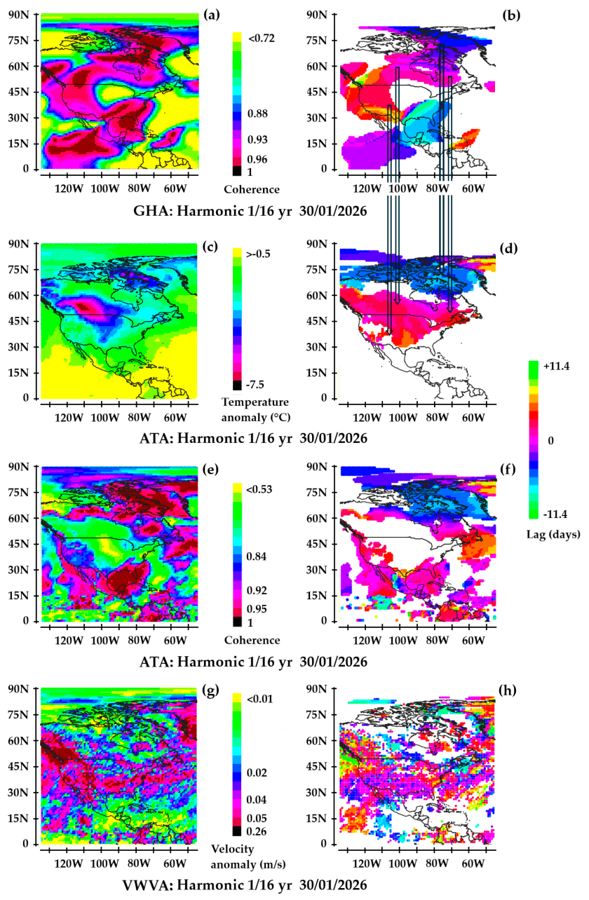
Figure 5.
Amplitude (a) and phase (b) of geostrophic wind velocities at the tropopause (250 hPa level) in the 17.1–34.2-day period band. The temporal reference is the wind velocity at 250 hPa, 70°N, 10°E. The observation date (28/05/2026) corresponds to the maximum of the temporal reference. The phase is displayed where the amplitude is significant (>6 m/s).
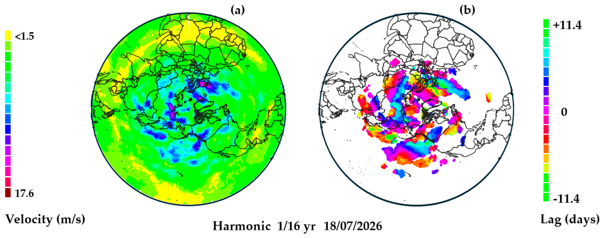
Figure 6.
(a-c), (g-i), (m-o), (s-u): geostrophic wind velocity anomalies (m/s) at the 250 hPa level in the 17.1-34.2-day period band – (d-f), (j-l), (p-r), (v-x): geopotential height anomalies (m) at the 500 hPa level in the same period band. The first column shows the amplitude, the second the coherence, and the third the lag in days. The phase is displayed where the amplitude is significant. The observation dates correspond to the maxima of the temporal reference.
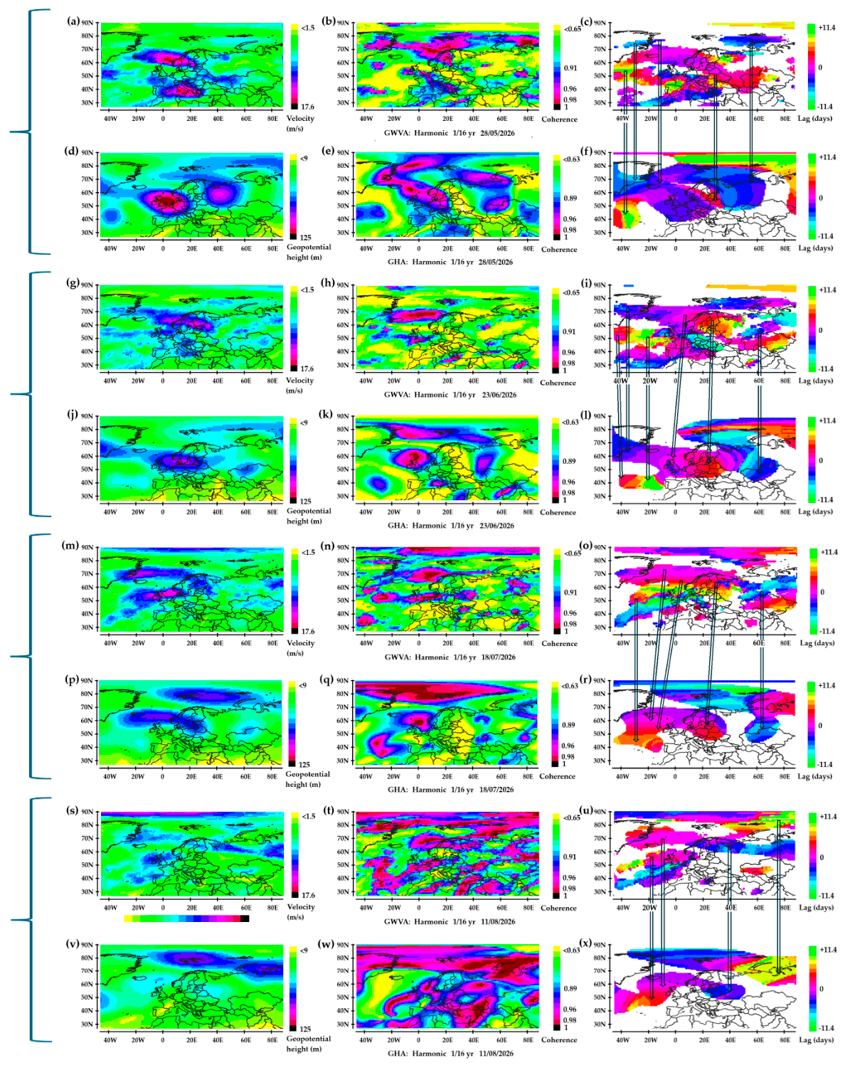
Figure 7.
Air temperature (°C) above 2 m in the 17.1-34.2 day period band. Amplitude (°C) in the first column, phase in the second column. The phase is displayed where the amplitude exceeds 2.0 °C. Same reference as in Figure 5.
Figure 7.
Air temperature (°C) above 2 m in the 17.1-34.2 day period band. Amplitude (°C) in the first column, phase in the second column. The phase is displayed where the amplitude exceeds 2.0 °C. Same reference as in Figure 5.
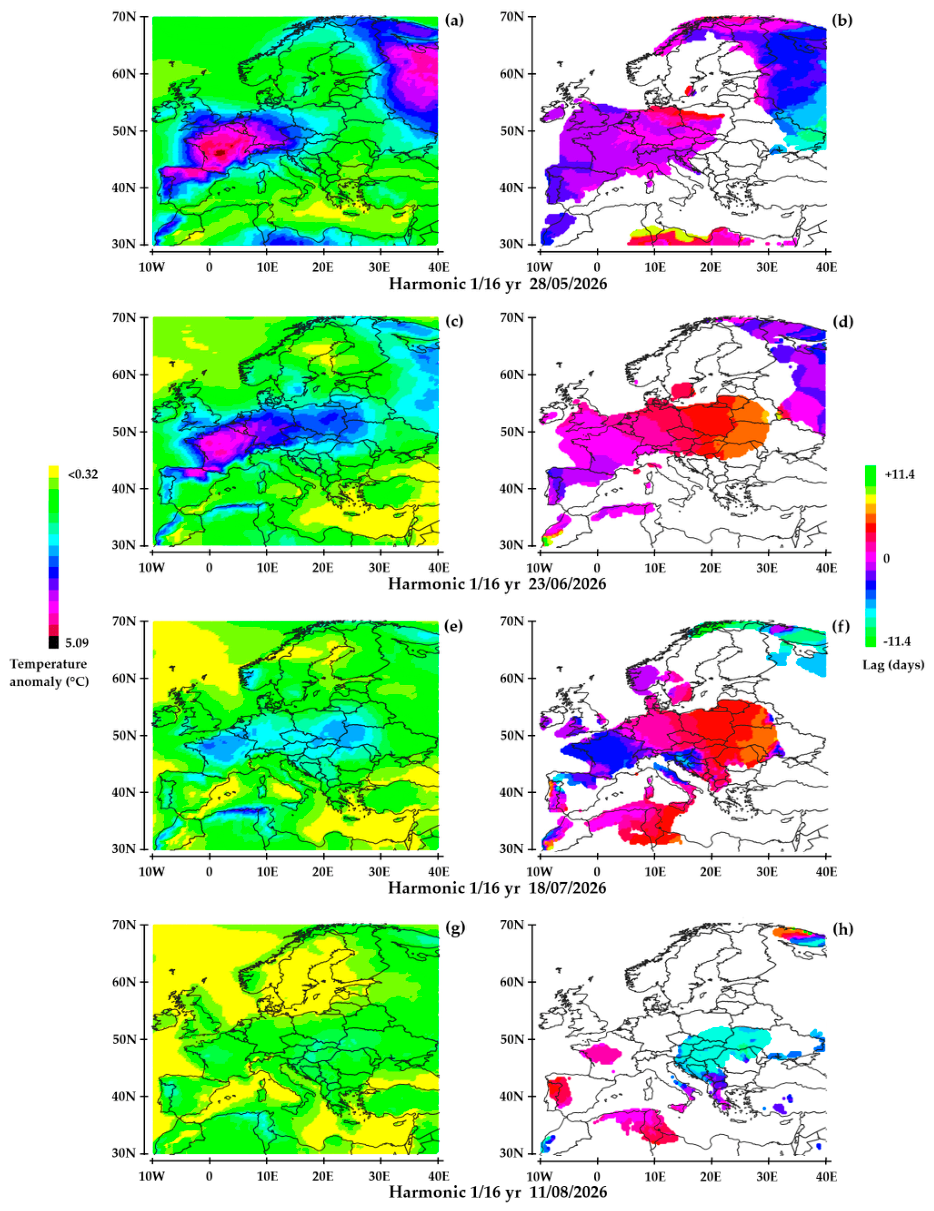
Figure 8.
Amplitude (a) and phase (b) of geostrophic wind velocities at the tropopause (250 hPa level) in the 8.6–17.1-day period band. The temporal reference is the same as in Figure 5. The observation date (30/05/2026) corresponds to a maximum of the temporal reference. The phase is displayed where the amplitude is significant (>7 m/s).
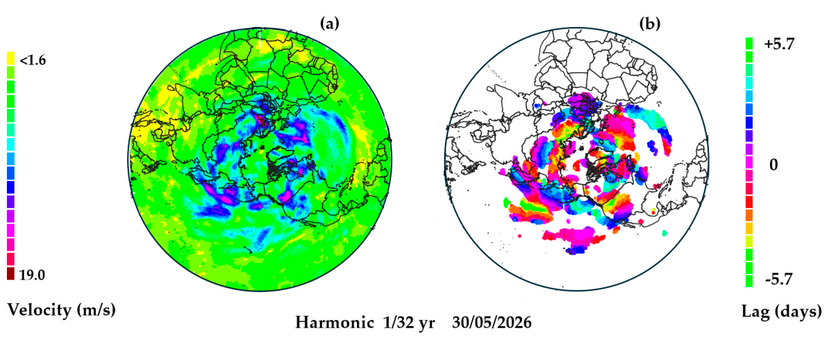
Figure 9.
(a-c), (g-i), (m-o), (s-u): geostrophic wind velocity anomalies (m/s) at the 250 hPa level in the 8.6-17.1-day period band - (d-f), (j-l), (p-r), (v-x): geopotential height anomalies (m) at the 500 hPa level in the same period band. The first column shows the amplitude, the second the coherence, and the third the lag in days. The phase is displayed where the amplitude is significant. The observation dates correspond to the maxima of the temporal reference.
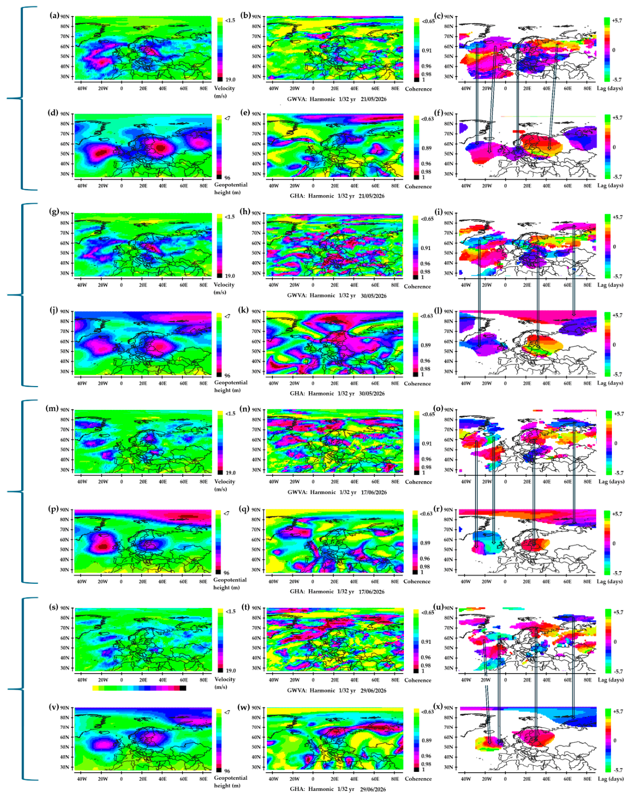
Figure 10.
Air temperature (°C) above 2 m in the 8.6-17.1 day period band. Amplitude (°C) in the first column, phase in the second column. The phase is displayed where the amplitude exceeds 1.6 °C.
Figure 10.
Air temperature (°C) above 2 m in the 8.6-17.1 day period band. Amplitude (°C) in the first column, phase in the second column. The phase is displayed where the amplitude exceeds 1.6 °C.
Disclaimer/Publisher’s Note: The statements, opinions and data contained in all publications are solely those of the individual author(s) and contributor(s) and not of MDPI and/or the editor(s). MDPI and/or the editor(s) disclaim responsibility for any injury to people or property resulting from any ideas, methods, instructions or products referred to in the content. |
© 2026 by the authors. Licensee MDPI, Basel, Switzerland. This article is an open access article distributed under the terms and conditions of the Creative Commons Attribution (CC BY) license (http://creativecommons.org/licenses/by/4.0/).
Copyright: This open access article is published under a Creative Commons CC BY 4.0 license, which permit the free download, distribution, and reuse, provided that the author and preprint are cited in any reuse.