

Submitted:
16 October 2026
Posted:
19 October 2026
You are already at the latest version
Abstract
Published rankings of GeoServer, MapServer and QGIS Server usually rest on one hand-tuned configuration per server under closed-loop load. Under a time-stamped protocol, 816 Sobol-sampled sessions per platform ran under open-loop load on exclusive nodes of two processor generations. Surrogates gave sensitivity indices and ranking probabilities. For capacity, the engine's total-order index (0.11) was below those of data complexity, image size, core count and request projection; latency was dominated by data complexity, image size and, for tail latency, the request projection. GeoServer had higher capacity than MapServer in 56% of the space, and capacity rankings reversed in 31% of workload cells on one platform and 35 to 41% for every pair on the other. At half its own capacity, GeoServer usually had the lowest median latency but the greatest relative tail inflation. The FastCGI worker count changed MapServer and QGIS Server capacity about 5.5-fold, and reprojection cost 30 to 69%. Surrogates did not transfer between processor generations. With 32 Bayesian-optimisation proposals each, GeoServer and MapServer tied within measurement resolution at a reference workload and QGIS Server reached 18% less. Rankings depended on configuration within the tested space, so benchmarks should sample configurations, use open-loop load and verify output equivalence.
Keywords:
WebGIS
; Web Map Service
; performance benchmarking
; GeoServer
; MapServer
; QGIS Server
; global sensitivity analysis
; Bayesian optimisation
; open-loop load
; reproducibility
1. Introduction
A Web Map Service (WMS) renders maps on request from spatial data and returns them as images [1]. GeoServer, MapServer and QGIS Server are open-source implementations of this interface, and each can be run with different data stores, process models, thread and worker limits and memory settings. People who choose between them, or size a deployment, want to know how quickly a server answers and how much load it carries before it saturates. Performance has been a concern of web geographic information systems (GIS) for as long as they have existed [2].
Published comparisons mostly answer that question for one configuration per server. Such a comparison confounds the server with its tuning, and the literature on configuration tuning shows why that matters: defaults routinely leave large gains unused in application servers, Java garbage collectors and databases [3,4,5]. Three further features limit what single-configuration results can support. Load is usually generated by a fixed number of virtual users, a closed-loop model in which the generator slows its own arrivals when the server slows down; open and closed models can lead to different conclusions about the same system, and closed loops understate tail latency [6,7,8]. Measurements usually come from one machine, so hardware variability is rarely observed, although it is substantial on nominally identical nodes [9,10]. And the outputs are rarely compared, so a faster server may simply be doing less work.
The stakes go beyond choosing a server. Published rankings are used to choose software for spatial data infrastructures, to size hardware, and as baselines in later research. If a ranking depends on configuration, workload or hardware more than on the server itself, a single-configuration benchmark can be correct for its own test and still misleading as general advice. Whether that happens, and how often, is an empirical question that no earlier study of these servers has been designed to answer. The answer matters in practice because the settings in question are cheap to change: a worker count or a request coordinate reference system (CRS) can be adjusted in minutes, whereas a change of server is a migration.
This study treats configuration as a sampled factor space. Each session runs a self-contained stack (PostGIS, one of the three servers, and an open-loop load generator) on an exclusive node of the Politecnico di Torino high-performance computing (HPC) cluster. Configurations are drawn from a scrambled Sobol design over server settings, database settings, data complexity, request properties and central processing unit (CPU) envelope. Each session measures latency against offered arrival rate, locates the saturation point of the configuration, and records whether the servers render equivalent maps. We ask five questions.
Research question 1 (RQ1, variance attribution): what share of the variance in log median (p50) latency, log 99th-percentile (p99) latency and log capacity is attributable to the server, its configuration, the database configuration, data complexity, request properties and the CPU envelope? RQ2 (ranking robustness): for each pair of servers, how often does one outperform the other across the configuration space, and where does the ranking reverse? RQ3 (tuned ceiling): what is each server’s best capacity under an identical tuning budget? RQ4 (tail and capacity under open load): how do latency curves, saturation points and tail inflation differ by server and configuration? RQ5 (transfer): do models trained on one hardware platform predict a second platform within their prediction intervals?
The protocol, factor space, session designs and code were frozen and time-stamped before the first campaign job was submitted, and the protocol is registered on the Open Science Framework (https://osf.io/uhrax/) [11]. The registration was filed after data collection had started, and part of the registered analysis was implemented after the data had been seen, so the registration documents the plan without making every analysis confirmatory; Section 3.9 reports these and every other deviation. A companion study (Study 2) is planned as a separate fixed-configuration benchmark on other hardware. It is intended as a confirmatory test of the models reported here and has not yet produced results.
Our contributions are: (i) a benchmark protocol for web map servers that samples configurations, generates open-loop load checked against server-side sojourn times on every platform, and verifies that the servers render equivalent maps; (ii) to our knowledge, the first benchmark of GeoServer, MapServer and QGIS Server WMS GetMap that samples their configuration space with a space-filling design and separates the effect of the server from the effect of configuration and workload; (iii) a variance decomposition and ranking-reversal analysis over the configuration space; (iv) an equal-budget tuning comparison and a cross-platform transfer test; and (v) a time-stamped reproducibility package. The novelty claim in (ii) is limited to these three servers and this service: designed experiments, open-loop load and surrogate-based sensitivity analysis are established methods elsewhere in systems research [12,13,14].
2. Related Work
2.1. Performance of Web Map and Geospatial Servers
A first group of studies measures services as they are operated. Horák et al. tested two Czech map services of INSPIRE (Infrastructure for Spatial Information in the European Community) with concurrent virtual users over two months [15] and later monitored download services with millions of random requests [16]. Wu et al. monitored the quality of public WMS resources to support map composition [17], Gui et al. surveyed and monitored 46,296 public WMS instances and found power-law response times that grow with distance to the server [18], and Xia et al. built a spatiotemporal performance model from distributed monitoring [19]. These studies describe the services that users actually meet, but they cannot separate the server software from its configuration, its data or its hosting.
A second group compares servers or settings under controlled load. Birgoren and Gumusay compared GeoServer, MapServer and ArcGIS Server on two imagery scenarios [20], and Masó et al. evaluated seven map server implementations under concurrent users [21]. Giuliani et al. tested the Web Feature Service (WFS) and Web Coverage Service (WCS) in GeoServer and ArcGIS Server, changing the data store, geometry, indexing, output format and resolution one factor at a time, and found that memory tuning and spatial indexing mattered more than the defaults suggested [22]. Růžička compared GeoServer WMS on a Shapefile and on PostGIS [23], and Cibulka showed that WMS response time varies with map position and scale, so that a single global indicator is not enough [24]. Dawid and Pokonieczny compared map generation time in GeoServer and MapServer while varying the area, the number of simultaneous requests and the number of layers, and found GeoServer faster in nearly all cases [25]. Tiwari et al. benchmarked a GeoServer stack for WMS, WFS, WCS and sensor services at 1,000 to 3,000 users [26], Liu et al. proposed a WFS benchmark of eleven queries on GeoServer [27], and Zhang et al. improved a GeoServer deployment by tuning the Java virtual machine (JVM) and caching [28], an early example of configuration mattering for these servers.
Other work covers sensor observation services, comparing three implementations including MapServer [29], web processing services [30], the istSOS sensor observation service under high load with request mixes taken from production logs [31], vector against raster tiles [32,33], and the newer implementations of the Open Geospatial Consortium (OGC) application programming interface (API) standards [34,35]. Infrastructure studies have examined cloud deployment of spatial web portals [36], tile services and containerised web GIS on clusters [37,38], clustered PostGIS geoservices [39], tile caching with trace-driven replay [40] and load balancing for concurrent WMS access [41].
Configuration-aware comparisons of GeoServer and MapServer exist mainly as grey literature. A presentation at the Free and Open Source Software for Geospatial (FOSS4G) conference of 2007 varied the data source, concurrency, Java and servlet container for GeoServer and the Common Gateway Interface (CGI) against FastCGI for MapServer [42], and the FOSS4G 2010 exercise compared MapServer, GeoServer, QGIS mapserver and other servers under JMeter thread counts of 1 to 64, with a baseline and a best-effort tuned scenario [43]. These exercises are the closest precedent for RQ3, but they used one tuned configuration per server and closed-loop load.
In the controlled comparisons of these servers, configuration is either fixed or varied one factor at a time and load is generated by a fixed number of concurrent clients. Some studies use several machines, for clustered deployments [21,39] or distributed monitoring [18,19], but none of those we reviewed tests whether a ranking between servers holds on other hardware. We found no study that samples the configuration space of these servers with a space-filling design, decomposes the variance of their performance, tests whether their rankings reverse across that space, compares them under an equal tuning budget, or tests whether results transfer across hardware. QGIS Server, in particular, is almost absent from peer-reviewed load tests. A Scopus search of titles, abstracts and keywords on 14 October 2026 combining the three server names with performance terms returned 62 records, none of which mentions QGIS Server in its title, abstract or keywords; a second search combining map-server terms with experimental-design, sensitivity-analysis, surrogate-model, Bayesian-optimisation and open-loop terms returned one record, which does not concern server performance. No title or abstract among the 62 records reports a designed factor space, open-loop load or a variance decomposition for these servers. The queries and the screened records are in the reproducibility package.
2.2. Load Generation and Latency Measurement
Banga and Druschel showed that common web benchmarks could not generate request rates beyond a server’s capacity, because their clients wait for responses [44]. Schroeder et al. compared open and closed workload models and showed that they can lead to very different conclusions about the same system [6]. Zhang et al. found that load testers whose blocking workers behave like a closed loop systematically underestimate tail latency [7]. The effect, known as coordinated omission, has been documented in database benchmarking [8,45], and it is avoided by issuing requests on a fixed schedule and timing each one from its intended send time [46]. Open-loop tools such as Mutilate and Lancet put this into practice and check that the client is not the bottleneck [14,47]. Tail percentiles rather than means are the relevant outcome because rare slow responses dominate what users see [48], and queueing theory explains why latency rises sharply as the arrival rate approaches capacity [49,50].
Steady state cannot be assumed after a fixed warm-up, particularly on the JVM: start-up and steady-state performance are different regimes [51], and changepoint analysis has shown that many benchmarks warm up irregularly or never stabilise [52,53]. We therefore detect the end of warm-up with a penalised changepoint method [54,55] and keep launches that never stabilise, labelled as such.
2.3. Performance Models of Configurable Systems
Predicting the performance of configurable software from a sample of measured configurations is an established line of software-engineering research, reviewed by Pereira et al. [13]. Performance-influence models relate options and their interactions to performance [12], and learners range from regression trees [56] to deep sparse networks [57]. Nair et al. showed that a model which ranks configurations correctly can find good ones even when its absolute predictions are poor [58,59], which motivates our attention to rankings and their reversals. Workloads interact with configuration options, often non-monotonically [60], so we sample workload properties alongside configuration. Performance models can be transferred between hardware platforms through simple mappings [61,62], and knowledge from one environment can guide sampling in another [63]; RQ5 tests a calibration-based transfer of this kind. Surrogate-based variance decomposition has also been used to measure which hyperparameters matter in machine learning [64]. We apply these ideas to map servers, where they have not been used.
2.4. Configuration Tuning and Equal-Budget Comparison
Automatic tuning has repeatedly shown that default settings leave large gains unused, in application servers [3], Java garbage collectors [4], Tomcat and other systems [65] and database management systems [5,66,67]. Bayesian optimisation [68,69,70] is a standard tool when each evaluation is expensive, as in CherryPick and BOAT [71,72]. Database studies suggest that a few influential settings capture most of the attainable gain [67,73], and that the choice of surrogate matters when the space contains categorical settings [74]. In machine learning, comparisons in which methods received unequal tuning effort produced rankings that changed once the budget was equalised [75,76], and the randomness of tuning is itself a source of variance [77]. RQ3 applies the same principle to map servers: each server receives the same optimisation budget, search procedure and confirmation replicates.
2.5. Variability, Reproducibility and Pre-Registration
Performance varies between runs and between nominally identical nodes on HPC systems [9,78] and in testbeds and clouds [10,79], and several authors have set out rules for repetition, statistical reporting and disclosure [80,81,82]. Repeatability of systems research depends on sharing artifacts [83], and reproducibility in GIScience has been found to be low in practice [84,85,86]. Pre-registration separates planned analyses from analyses chosen after seeing the data [11], and registered reports have been adopted in software engineering [87]. Our design follows these recommendations: exclusive nodes, calibration measurements, replicate jobs on different nodes, containers pinned by digest [88,89], a manifest anchored by decentralised trusted timestamping [90], and a public registration.
3. Materials and Methods
3.1. Study Design and Registration
The design, configuration, code, analysis plan and remaining protocol decisions were frozen on 25 September 2026 at 08:56 Coordinated Universal Time (UTC), before the first campaign job was submitted. The freeze manifest lists the SHA-256 hash (Secure Hash Algorithm 2 and Algorithm 256-bit digest) of 1,701 files, including all benchmark code, the factor space, the campaign protocol and both design files with every session configuration. The manifest hash (98662fc9...b649) carries an OpenTimestamps proof anchored in the Bitcoin blockchain. The analysis code was written after the freeze, validated on simulated campaigns with known truth, and installed on the cluster at 09:17 UTC, before any campaign session had started; its record carries its own proof. Both hashes and proofs are in the registration and the reproducibility package.
Data collection began after the freeze and before the registration was filed on 29 September 2026. Until filing, only operational health was inspected: job state, failures, node admission, manipulation-check outcome and wall time. The report script refused to run until the filing was recorded on the cluster. No null-hypothesis tests are planned; results are reported as point estimates with 95% intervals.
3.2. Platforms
The primary platform is the Legion cpu_sapphire partition (Intel Xeon Gold 6442Y, 2 x 24 cores, simultaneous multithreading (SMT) enabled with one thread per core used, 2 non-uniform memory access (NUMA) nodes, 503 GiB). The secondary platform is cpu_skylake (Intel Xeon Gold 6130, 2 x 16 cores, no SMT, 2 NUMA nodes, 376 GiB). Every session runs on an exclusive node. One four-socket cpu_sapphire node is excluded so that the primary platform keeps the two-socket topology of the pilot nodes. CPU model, frequency settings and calibration scores are recorded for every session because nominally identical nodes can differ: in the pilot, one cpu_skylake node scored 1.65 ns on the integer calibration against 2.16 ns on the other five and reached a higher capacity. Calibration therefore enters the transfer analysis of RQ5 as a scaling adjustment and defines the node sensitivity analysis (Section 3.8).
3.3. Software Stack and Isolation
Each session runs PostgreSQL 17.5 with PostGIS 3.5.2, one of GeoServer 2.28.3, MapServer 8.6.6 or QGIS Server 3.44.9, and an open-loop load generator, communicating over loopback. Components are pinned to disjoint CPU sets (server, database, load generator, housekeeping), with one hardware thread per core and the load generator on a different NUMA node; all data sit on node-local disk. Container images are pinned by digest and run as Singularity Image Format (SIF) files with Apptainer 1.4, the successor of Singularity [89]. MapServer and QGIS Server sit behind the same nginx front with the same settings; GeoServer uses its embedded Tomcat connector. No server writes per-request access logs, and every server returns 24-bit red-green-blue (RGB) Portable Network Graphics (PNG) images. GeoServer runs on Java Development Kit (JDK) 17. The PostGIS image is built on Debian bullseye with GEOS 3.9 and PROJ 7.2.
3.4. Data and Requests
The data are deterministic synthetic polygons over a 400 x 300 km extent in EPSG:3035 (the European Petroleum Survey Group code for the Lambert azimuthal equal-area projection of Europe): two layers of 100,000 polygons each, with 16 and 256 vertices per polygon. The generator uses fixed seeds and the stream hash is recorded. Tables are clustered on their generalised search tree (GiST) index and frozen with VACUUM FREEZE, so every restored copy is physically identical. Requests are WMS 1.3.0 GetMap [1] in EPSG:3035 or EPSG:3857, with axis order taken from the CRS definition. A sequence of 2,000 deterministic bounding boxes with map widths of 2, 10 and 50 km is sent identically to every server.
3.5. Factors and Sampling
The common factors are the layer, image size (256, 512 or 1024 px), request CRS, number of server cores (2, 4, 8 or 16) and PostgreSQL shared_buffers. Each server adds its own factors (Table 1). Configurations are drawn from a scrambled Sobol design [91,92] per server (seed 2026), with 256 configurations per server. Eight anchor configurations per server receive three replicate jobs each, which gives 816 sessions per platform. A session is one job that runs one configuration; it contains two launches, each a cold start of the stack followed by a load ladder (Section 3.6). The anchors are the replicated sessions that inform the noise model. The same 768 configurations and the same anchors run on both platforms. Because the first 2^k points of the design are balanced, the campaign runs in file order and analysis can start at any power of two.
3.6. Measurement Protocol
Before anything starts, the job checks that the node resolves the user’s uid and that the node spends at most 10% of its CPU time busy over 5 s; a node that fails is recorded, excluded from later submissions, and the job is resubmitted elsewhere. The session then runs integer, fused multiply-add (FMA), memory-bandwidth and memory-latency microbenchmarks once on one core of each CPU set. Each launch starts the database and server cold and applies a manipulation check that reads every factor back from the running system (PostgreSQL settings, JVM heap and collector, Tomcat limits, GeoServer pool size, FastCGI and nginx worker counts, CPU affinity of every process, and the image size and CRS of the request stream). A mismatch aborts the session before load is applied. A probe pass of 200 sequential requests records output fingerprints and keeps the first 64 bodies. Warm-up applies open-loop load at 30% of estimated capacity until a penalised changepoint search [54] on 5 s window medians of log latency finds a steady state, for at most 900 s; launches that do not reach one are labelled no_steady_state and kept.
The load ladder uses constant-arrival-rate levels of 60 s on a geometric grid of 1.5^(k/4) requests per second, rising by a factor of 1.5 until a level saturates, followed by geometric bisections on the same grid. The registered protocol set three bisections to bracket the knee to half a grid step (factor 1.052); the ladder code stops after two, at one grid step (factor 1.107), as Section 3.9 reports. A level is saturated if the error rate exceeds 1%, achieved over offered throughput falls below 0.95, any iteration is dropped, or p99 exceeds 10 s. After each saturated level a recovery gate sends single requests until five consecutive responses succeed within max(3 x probe median, probe median + 50 ms), for at most 180 s; if the server does not recover, the ladder stops. Server logs are scanned after every level for out-of-memory errors, garbage-collector warnings, lost FastCGI workers and segmentation faults. A post-probe repeats the first 64 requests to confirm that outputs did not change. Each job runs two cold launches, and replicate jobs run on different nodes.
The latency of record is the open-loop iteration duration, from scheduled arrival to last byte, with queueing included [6,46]. A request fails if its status is not 200, it times out after 30 s, or its content type is not image/png. Before data from a platform are accepted, the load generator must match server-side sojourn times within max(2 ms, 2%) at p50, p90, p99 and p99.9 (the 50th, 90th, 99th and 99.9th percentiles) on a reference single-queue server. The checks passed on both platforms (client minus server p99 of 0.18 to 0.62 ms), while a closed-loop generator understated p99 by a factor of 54 to 57 on the same server.
3.7. Outcomes
Capacity (Y1) is the highest unsaturated grid rate, with its bracket; because the request stream mixes all three map widths, it is the capacity for that mixed workload. Latency (Y2) is log p50 and log p99 at 25%, 50% and 75% of each launch’s own knee, taken as the lower end of its bracket, interpolated linearly in log rate without extrapolation. Configurations are therefore compared at the same fraction of their own capacity, not at the same offered rate. Tail inflation (Y3) is log(p99/p50) at 50% of the knee. Overload robustness (Y4) is whether the server recovers after its first saturated level, the recovery time, and fault counts from the server log. Validity covariates are output equivalence, measured as the intersection over union (IoU, also called the Jaccard index) of ink masks [93] and the structural similarity index (SSIM) [94] against the other servers by map width, the warm-up label, calibration scores and generator health.
3.8. Analysis
A load level is invalid if the load-generator CPU set averages above 80% utilisation or, for an unsaturated level, if schedule lag p99 exceeds 10 ms. Launches are excluded if the session manifest does not verify or if the server or database cores show more than 5% or 25% of CPU time not used by the benchmark’s own processes. Every exclusion is reported with its count. Session outcomes are means over valid launches. For the surrogates, a launch’s log capacity is the geometric midpoint of its knee bracket; for a one-step bracket this moves the value by about 0.05 at most. A bracket open at one end (a knee below the first rung or above the top rung) enters as its finite end, which is a bound rather than an estimate; this applies to five sessions.
Noise is modelled on the anchor sessions as log outcome ~ configuration + (1 | node) + (1 | job): one fixed mean for each anchor configuration, crossed random intercepts for node and job, and launch-to-launch variation as the residual. The model is fitted by restricted maximum likelihood (REML) [95], for each engine and for all engines together, and gives node, job and launch variance components. For each server and outcome a Gaussian process with an automatic relevance determination (ARD) kernel and a white-noise term estimated from the data serves as the surrogate [96]; gradient-boosted trees [97] with split-conformal intervals [98] serve as a robustness check, and out-of-sample error is reported on the anchors and a 10% random hold-out. Inputs map every factor to [0,1], with numeric levels on a log scale.
RQ1 estimates total-order Sobol indices [99,100] on the surrogate with the Saltelli estimator [101,102] and 2^12 base points, following the metamodel approach of Marrel et al. [103,104]. Intervals come from 200 bootstrap refits that resample configurations, keeping the replicates of an anchor together. The server term comes from a pooled surrogate with the server as a categorical input, restricted to the common factors. Total-order indices include each factor’s interactions, so they do not sum to one and are not exclusive shares; the server index measures how much of the variance of the pooled model, under the registered factor distribution, involves the server. RQ2 estimates the probability of superiority [105,106] from surrogate predictions on 2^14 Sobol points, over the common factors and each server’s own factor distribution. The reversal share is the probability mass of the 144 common-factor cells in which the expected difference in the log outcome has the opposite sign to the overall one; reversal regions are mapped by partial dependence.
RQ3 runs expected-improvement Bayesian optimisation [68] on the primary platform with an equal budget of 32 proposals per server. The search space is each server’s tunable factors (its own factors and shared_buffers) at the pilot reference workload (poly_v16, 512 px, EPSG:3035, 4 server cores). Each round refits a Gaussian process for log capacity on all sessions of the server, with workload factors as inputs so that batch 0 informs the fit, scores 4,096 Sobol candidates by expected improvement over the best posterior mean among evaluated reference-workload configurations, and picks four configurations by the kriging-believer rule [107]. The configuration with the best posterior mean (the selected configuration) is then re-run as three replicate jobs, and their mean is the confirmed capacity. These sessions are analysed separately from batch 0.
RQ4 models knee brackets with interval censoring [108]: log capacity lies between the last unsaturated and the first saturated rate, with a random intercept per job integrated out numerically, and a bracket open at one end is censored at that end. Because the launch residual is far smaller than the bracket width, the integrand is close to a box with sharp edges, which the registered Gauss-Hermite rule [109] does not resolve; the intercept is therefore integrated by composite Gauss-Legendre quadrature over each job’s region of support, with breakpoints at the bracket ends (Section 3.9). Standard errors are Wald errors from the observed information. Brackets are one grid step wide after bisection, and wider when the ladder stopped before bisection was complete, for example because the server did not recover, or when some of its levels were invalid; all enter the same likelihood.
RQ5 trains surrogates on cpu_sapphire and predicts every cpu_skylake session, with and without calibration. The calibrated prediction scales capacity by the ratio of integer calibration times of the two platforms and latency by its inverse, with elasticity 1. Coverage uses the 95% predictive interval including the noise term.
Sensitivity analyses exclude nodes whose calibration deviates by more than 10% from the platform median, exclude no_steady_state launches, and restrict the data to map widths with cross-server IoU of at least 0.90. In the pilot, median IoU over the three server pairs for poly_v16 was 0.99 at 2 km, 0.96 at 10 km and 0.86 at 50 km, so headline comparisons are reported overall and for the 2 and 10 km widths.
The registered stopping rule ended job submission at the first of three conditions: (a) for every engine and outcome, every factor with a total-order index of at least 0.05 had a 95% bootstrap interval with a half-width of at most 0.05; (b) for every engine, the median absolute error of the surrogate for log p99 at 50% of the knee on the random hold-out was at most 0.10; or (c) the cap of 700 node-hours per platform was reached.
All analyses ran inside the analysis container with Python 3.12.14, NumPy 2.4.4, SciPy 1.17.1, pandas 3.0.2, scikit-learn 1.8.0 and PyArrow 25.0.1; figures were drawn with Matplotlib 3.11.2.
3.9. Operational Events and Deviations
Two operational events affected the campaign. From 26 to 29 September the cluster home filesystem was over its quota and the campaign stopped until storage was restored, and on 25 and 26 September a fault in the cpu_sapphire controller made about 65 sessions run twice. Appendix A.1 describes both and how each was handled.
The registered text differs from the frozen draft only in decisions recorded at the freeze (16 server cores kept on cpu_skylake, a budget of 32, stopping thresholds of 0.05 and 0.10, a cap of 700 node-hours per platform), in running the full design on the secondary platform, in excluding the four-socket node and nodes without a container runtime while every job was still queued, and in adding the analysis specification before any data were read. The RQ3 rounds were driven by a script added to the code tree on 5 October 2026, which calls the frozen optimisation code without changing it.
After the first full report it became clear that the frozen report code implemented only part of the registered analysis plan: exclusions, RQ1 per engine, RQ2, RQ5, the hold-out errors and the stopping rule. The noise model, the RQ1 engine term, the boosted-tree check, RQ4, the sensitivity analyses and the equivalence report were added on 5 October 2026, after the data had been seen. They use the frozen and validated estimators (REML, interval-censored regression, Sobol indices, surrogate refits) and follow the registered specification; the new code was checked on simulated data before use. In addition, the frozen surrogates estimate their noise term from the data (a white-noise kernel) rather than taking it from the noise model as registered. The post hoc analyses without the database foreign-CPU rule (Section 4.7; RQ1 and RQ2 on 5 October, RQ4 on 8 October 2026) were not registered. Every file added after the freeze is listed with its SHA-256 and date in the reproducibility package.
Two further deviations were found when the RQ3 results were checked on 8 October 2026. First, the registered protocol specifies three geometric bisections that bracket the knee to half a grid step (factor 1.052). The frozen ladder code bisects only to points of the 1.5^(k/4) grid and stops once the bracket is one grid step wide, so the third bisection never ran. No launch in the main batch or in RQ3 had a bracket narrower than one grid step (factor 1.107). Of the valid launches, 1,350 of 1,534 on cpu_sapphire (88.0%) and 1,262 of 1,518 on cpu_skylake (83.1%) had a bracket of exactly one step; the rest were wider because the ladder stopped early or some of its levels were invalid. The analyses use the brackets as recorded, so the interval-censored model of RQ4 remains valid, with wider intervals than registered, but the bracket midpoints used by the surrogates carry about 0.05 of rounding in log capacity for a one-step bracket, and more for wider ones, rather than the registered 0.025; two sessions less than one step apart cannot be told apart. Second, the optimisation code counts proposals against the budget of 32, not valid evaluations, and configurations whose sessions have no valid launch never enter the Gaussian process; for MapServer this left 24 valid evaluations (Section 4.4).
Three further problems were found in an independent review of the analysis code on 13 and 14 October 2026. The first two were corrected by re-analysis and the results in Section 4 include those corrections; the effect of the third cannot be established. First, the archived interval-censored regression of RQ4 integrated the job intercept with 24 Gauss-Hermite nodes. The launch residual is far smaller than the 0.10-wide brackets, so the rule misestimated the log-likelihood at the published estimates by about 2 to 41 units. RQ4 was refitted with composite Gauss-Legendre quadrature, which agreed with an independent adaptive integration to about 10⁻¹² in log-likelihood at the estimates checked, and 62 of 63 fits from different starts reached the same optimum. Point estimates changed by at most 0.07 on cpu_sapphire and 0.09 on any dataset, but the published standard errors had been about ten times too small. Profile-likelihood intervals for every effect in Table 5 agreed with the Wald intervals to within 0.3% of their width; for the launch residual they were wider and asymmetric but bounded on both sides.
Second, the function that turns knee brackets into session capacities treated a missing bound passed as a floating-point NaN (not a number) as present, so five sessions with a bracket open at one end (one on cpu_sapphire, four on cpu_skylake) had no capacity and dropped out of every capacity model. With the registered treatment restored, all capacity analyses were rerun. Sensitivity indices, ranking probabilities, reversal shares and transfer errors moved by 0.007 or less, except the cpu_skylake pooled indices (engine 0.132 to 0.142, layer 0.260 to 0.246); the hold-out checks, which rest on few sessions, moved more (Section 4.1). With the uncorrected data the cpu_skylake pooled engine index depended on the node type and thread count used for the refit (0.132 on cpu_skylake nodes, 0.142 on cpu_sapphire nodes); with the corrected data it was 0.142 on both node types and at both thread counts tried.
Third, the same defect left the cpu_sapphire GeoServer session out of the training data of the GeoServer optimisation in RQ3. The RQ3 measurements are unaffected, but the effect of the omission on the proposals and on the selected configuration has not been established, and RQ3 reports the optimisation as it was run. The corrected code, the control runs and the comparisons are in the reproducibility package.
The Methods above describe the analysis as executed. It differs from the registered text in three further points: the calibration microbenchmarks run once per session rather than in every launch; latency is computed only at fractions of each launch’s own knee, not also at common offered rates; and calibration enters RQ5 and the node sensitivity analysis rather than the models as a covariate. The load-generator and schedule-lag rules invalidate individual load levels, as registered.
4. Results
Unless stated otherwise, results refer to the primary platform (cpu_sapphire). Effects on log capacity are given as multiplicative changes, exp(effect) - 1.
4.1. Campaign Summary and Data Quality
All 816 sessions per platform completed, each with two launches (1,632 per platform). On cpu_sapphire 1,534 launches (94.0%) were valid and 767 sessions had at least one valid launch; on cpu_skylake the figures were 1,518 (93.0%) and 759. Every such session has a capacity; five of them (one on cpu_sapphire, four on cpu_skylake) have a bracket open at one end and enter as its finite end. Capacity varied far more within each engine than between engines (Figure 1): across the sampled configurations it spanned a factor of 86 to 358 on cpu_sapphire, while the engine medians differed by at most 29%. No launch failed manifest verification or the manipulation check, and none showed foreign load on the server cores. Three launches per platform did not reach a steady state. Of the 13,098 load levels on cpu_sapphire, 2,209 (16.9%) were invalid because the schedule lag of an unsaturated level exceeded 10 ms; on cpu_skylake 3,385 of 13,728 levels were invalid (3,338 for lag and 53 for load-generator CPU, 6 of them for both). The registered stopping rule (Section 3.8) was met on cpu_sapphire for both criteria (a) and (b); on cpu_skylake criterion (a) was met, but criterion (b), the hold-out error of the p99 surrogate, was not met for MapServer and QGIS Server. Measured as session wall time from the per-session run records, the confirmatory batch used 301 node-hours on cpu_sapphire and 332 on cpu_skylake, and pilot and test sessions a further 36; RQ3 added 40 node-hours in 102 session jobs.
All launch exclusions came from one rule: more than 25% of CPU time on the database cores not accounted for by the benchmark’s processes (98 launches on cpu_sapphire, 114 on cpu_skylake). These exclusions were not spread evenly. On cpu_sapphire they removed 4.4% of GeoServer launches, 13.6% of MapServer launches and no QGIS Server launch. All 24 GeoServer exclusions lay in the top quartile of GeoServer capacity, where they removed 19% of launches. All 74 MapServer exclusions came from configurations that close the database connection after every request, and 46 of them lay in the top quartile of MapServer capacity, where they removed 38% of launches. The rule therefore did not detect foreign load, as intended; it picked up database work that no benchmark process accounts for, consistent with kernel network work that grows with throughput for GeoServer and with the setting up of a new connection for every request for MapServer. As a result, 12 GeoServer and 37 MapServer sessions had no valid launch, leaving 244, 221 and 256 configurations for GeoServer, MapServer and QGIS Server. We report the registered analysis and, in Section 4.7, post hoc analyses without this rule.
Measurement noise was small. On the anchor configurations of cpu_sapphire, the REML noise model gave a launch-to-launch standard deviation of 0.044 in log capacity (about 4.5%), with node and job components close to zero (Table 2). On cpu_skylake the node and job components were larger (0.07 and 0.09 in log capacity), consistent with the calibration differences between nominally identical nodes described in Section 3.2. The surrogates predicted held-out configurations well: on cpu_sapphire the median absolute error in log capacity was 0.04 (GeoServer and MapServer) and 0.07 (QGIS Server), and in log p99 at 50% of the knee 0.03 to 0.05. Gradient-boosted trees were less accurate (0.06 to 0.15 in log capacity), their split-conformal intervals covered 90 to 100% of the random hold-out configurations for the three outcomes (21 to 25 per engine and outcome; 85 to 100% on cpu_skylake), and they ranked the four most important factors identically to the Gaussian processes in eight of nine engine and outcome combinations (the ninth differed only in fourth place).
The three engines drew practically the same maps at the two smaller map widths. Across all engine pairs, the median ink-mask IoU was 0.94 to 0.98 at 2 and 10 km, and 96 to 100% of image pairs reached an IoU of at least 0.90. At 50 km the median IoU was 0.87 to 0.92 and only 33 to 58% of pairs reached 0.90, as in the pilot, so the equivalent-work stratum is the 2 and 10 km widths. Capacity is measured on the mixed stream of all three widths and cannot be restricted to this stratum after the fact.
4.2. RQ1: Variance Attribution
The choice of engine was a minor factor. In the pooled surrogate over the common factors, the total-order index of the engine was 0.11 (95% interval 0.10 to 0.20) for log capacity, 0.13 (0.13 to 0.16) for log p50 and 0.11 (0.11 to 0.12) for log p99 at 50% of the knee (Table 3). For capacity, the data layer (0.29), image size (0.26), number of server cores (0.25) and request CRS (0.20) each had a larger total-order index than the engine; because the indices include interactions, they sum to about 1.1. For latency the data layer and image size dominated p50 (0.38 and 0.49), the data layer and request CRS dominated p99 (0.42 and 0.36, image size 0.24), and the number of cores hardly mattered (0.00 and 0.03). On cpu_skylake the engine index was of the same order: 0.14 (0.13 to 0.25) for log capacity, 0.08 (0.08 to 0.12) for log p50 and 0.17 (0.16 to 0.18) for log p99.
Within each engine the picture differed (Figure 2). GeoServer capacity depended on the number of cores (total-order index 0.38), the request CRS (0.37), image size (0.17) and layer (0.12); its own settings (heap, garbage collector, Tomcat threads, connection pool) each explained less than 1%. MapServer capacity depended on the layer (0.35), the number of FastCGI workers (0.33), image size (0.18) and cores (0.17), and QGIS Server capacity on the number of FastCGI workers (0.30), image size (0.26), layer (0.20), cores (0.19) and CRS (0.13). PostgreSQL shared_buffers explained less than 0.1% of the variance in capacity for every engine, although the interval-censored model (Section 4.5) shows a small positive effect for GeoServer (+0.14 on the log scale over the full range).
4.3. RQ2: Ranking Robustness
No engine had the highest capacity everywhere (Table 4). On cpu_sapphire GeoServer had higher capacity than MapServer in 56% of the factor space (95% interval 53 to 58%), and the sign of the expected difference in log capacity was reversed in 31% of the common-factor cells. GeoServer outperformed QGIS Server in 74% of the space (reversal share 15%) and MapServer outperformed QGIS Server in 66% (24%). On cpu_skylake the rankings were weaker still: 58%, 62% and 56%, with reversal shares of 35%, 36% and 41%.
Median latency at 50% of each configuration’s own knee was more consistent. For latency, a reversal is a workload cell in which the mean difference in log latency has the opposite sign to the overall one. GeoServer had the lower p50 in 88% of the space against MapServer and in 98% against QGIS Server. Its tail was proportionally heavier, however: the ratio of p99 to p50 was higher for GeoServer than for MapServer in 81% of the space and than for QGIS Server in 90%. For p99 itself the result depended on map width. Over all widths GeoServer had the lower p99 in 63% of the space against MapServer, but where it was slower it was slower by a large margin, so the mean difference favoured MapServer. Restricted to the equivalent-work stratum of 2 and 10 km maps, GeoServer had the lower p99 in 77% of the space against MapServer and 92% against QGIS Server, with reversal shares of 21% and 2%.
Figure 3 shows the same probabilities with their 95% bootstrap intervals. The reversal share is defined relative to the sign of the mean difference in the log outcome, so it can exceed 0.5 when one engine wins most of the space by small margins and loses the rest by large ones, as for p99 between GeoServer and MapServer.
4.4. RQ3: Tuned Ceiling
The optimisation used 102 session jobs between 5 and 8 October 2026, and every job completed at its first attempt. At the reference workload almost every configuration proposed for an engine fell into a single capacity bracket (Figure 4): all 32 for GeoServer (291.9 to 323.1 requests/s), all 32 for QGIS Server (238.4 to 263.8 requests/s) and 23 of the 24 valid MapServer configurations (291.9 to 323.1 requests/s); the remaining MapServer configuration closed the database connection after every request and fell one step lower. Both launches of the three confirmation replicates of each engine’s selected configuration fell into its bracket, so the confirmed capacity, taken as the bracket midpoint, is 307.1 requests/s for GeoServer and MapServer and 250.8 requests/s for QGIS Server. The tuned GeoServer and MapServer are tied within the resolution of the ladder, and the tuned QGIS Server is 18% lower. Because the proposals were tied, the selected configurations, listed in Appendix A.2, have no measured advantage over the other configurations.
The best main-batch sessions at the same workload reached 277.5, 307.1 and 250.8 requests/s. The tuned GeoServer was therefore one grid step (11%) above the best main-batch GeoServer session, while MapServer and QGIS Server were unchanged, which turned a one-step lead of MapServer over GeoServer into a tie. The main-batch sessions ran in an earlier campaign, so part of this step may reflect the campaigns rather than the tuning. The GeoServer proposals differed from the main-batch sessions in collector, shared_buffers and pool size at once, so these data do not show which setting produced the gap (Appendix A.2).
MapServer received 24 valid evaluations instead of 32. Five of its configurations failed the database foreign-CPU rule of Section 4.1, and the optimisation code proposed three of them again without running them a second time (Section 3.9). All five had their knee one step below the selected configuration, so none would have exceeded its bracket.
4.5. RQ4: Tail and Capacity Under Open Load
The interval-censored model gave the main effects of each factor on log capacity, over its full registered range (Table 5). Going from 2 to 16 server cores multiplied capacity by 5.4 for GeoServer, 2.3 for MapServer and 3.1 for QGIS Server. Going from 1 to 64 FastCGI workers multiplied capacity by 5.5 for both MapServer and QGIS Server. Requests in EPSG:3857, which the engines reproject from the EPSG:3035 data, reduced capacity by 69% for GeoServer, 29.5% for MapServer and 54% for QGIS Server. Closing the database connection after every request cost MapServer 21% (16% in the post hoc fit without the database rule, Section 4.7), and parallel rendering cost QGIS Server 11%. Every effect named here is more than two model-based standard errors from zero; the weakest, parallel rendering, has a 95% interval for the capacity ratio of about 0.80 to 0.99 by both Wald and profile likelihood. The GeoServer collector, heap and Tomcat threads, shared_buffers and nginx workers for MapServer and QGIS Server, and the QGIS Server rendering threads were within two standard errors of zero. The job-level random intercept (standard deviation 0.24 to 0.42) was much larger than the launch residual (about 0.001 to 0.008, below the resolution of the brackets and only loosely determined), which means that the configurations differ in ways a main-effects model does not capture; the interactions are what the surrogates in RQ1 and RQ2 describe.
Overload was handled well. After the first saturated level, GeoServer recovered in 99.8% of launches on both platforms and MapServer and QGIS Server in all launches, with a median recovery time of zero. GeoServer threw an OutOfMemoryError in 0.6% of launches. Tail inflation at 50% of the knee, measured as log(p99/p50), had a median of 1.69 for GeoServer, 1.47 for MapServer and 1.33 for QGIS Server on cpu_sapphire, so p99 was typically 5.4, 4.3 and 3.8 times the median. Median latency stayed within about 12% of its lowest-load value up to 90% of the knee for all three engines, whereas p99 rose throughout the range and fastest for GeoServer (Figure 5).

Table 5.
Interval-censored regression of log capacity on the encoded factors with a random intercept per job, cpu_sapphire. Effects are for the full registered range of each factor (model-based Wald standard errors 0.03 to 0.09; profile-likelihood intervals agree with the Wald intervals to within 0.3% of their width).
Table 5.
Interval-censored regression of log capacity on the encoded factors with a random intercept per job, cpu_sapphire. Effects are for the full registered range of each factor (model-based Wald standard errors 0.03 to 0.09; profile-likelihood intervals agree with the Wald intervals to within 0.3% of their width).
| Factor (low to high) | GeoServer | MapServer | QGIS Server |
|---|---|---|---|
| Server cores (2 to 16) | +1.69 | +0.84 | +1.12 |
| FastCGI workers (1 to 64) | n/a | +1.70 | +1.70 |
| Image size (256 to 1024 px) | −0.96 | −1.08 | −1.47 |
| Layer (16 to 256 vertices) | −0.71 | −1.28 | −1.00 |
| CRS (3035 to 3857) | −1.18 | −0.35 | −0.78 |
| shared_buffers (512 MB to 8 GB) | +0.14 | +0.08 | +0.04 |
| Other engine setting (largest) | +0.15a | −0.24b | −0.12c |
a Connection pool size. b Closing the database connection after every request. c Parallel rendering.
4.6. RQ5: Transfer Across Platforms
Models trained on cpu_sapphire did not predict cpu_skylake within their intervals (Table 6). Without calibration, the median absolute error in log capacity was 0.58 for GeoServer, 0.59 for MapServer and 0.42 for QGIS Server, a factor of 1.5 to 1.8, and the 95% prediction intervals covered between 0% and 25% of sessions. Scaling by the ratio of integer calibration times roughly halved the error in log capacity (0.27 to 0.30) but coverage stayed below 20%. For latency the calibrated errors were 0.30 to 0.37 in log p50 and 0.26 to 0.37 in log p99. Within a platform the same surrogates were accurate (Section 4.1), so it is the tested surrogates and the calibration adjustment, not their fit within a platform, that failed to carry over. The two platforms differ in processor generation, core count, memory and node population, and these data cannot say which difference matters or whether a richer transfer model would succeed.
4.7. Sensitivity Analyses
No cpu_sapphire node deviated from the platform median calibration by more than 10%, so the first registered sensitivity analysis left the data unchanged. Excluding the three launches without a steady state did not change any index or probability at the reported precision. Restricting latency to 2 and 10 km maps strengthened GeoServer’s p99 advantage (Table 4) and left its p50 advantage almost unchanged (0.87 instead of 0.88 against MapServer, 1.00 instead of 0.98 against QGIS Server). It did change the order of the latency factors: the data layer and image size were the two most important factors for p50 and p99 of every engine, and the request CRS, which ranked first for GeoServer p99 and second for QGIS Server p99 over all widths, fell to third for both. In the post hoc analysis without the database foreign-CPU rule, 816 sessions entered the models and the probabilities of superiority for capacity changed by at most 0.013 (GeoServer against MapServer 0.572 instead of 0.559); the four most important factors per engine were unchanged. A second post hoc analysis, run on 8 October 2026, refitted the interval-censored model of RQ4 without the rule on all 1,632 launches: no main effect changed by more than about 0.06 on the log scale (largest 0.060, MapServer connection closing), and closing the database connection after every request still cost MapServer 16%. The bias described in Section 4.1 therefore did not alter any conclusion.
5. Discussion
5.1. What a Single-Configuration Benchmark Can and Cannot Show
On both platforms the total-order index of the engine was 0.08 to 0.17 for capacity and latency. For capacity the data layer, image size, number of cores and request CRS each mattered more than the engine; for latency the data layer and image size did, joined by the request CRS for p99, and the number of cores mattered little. Within each engine only a few settings mattered: the number of FastCGI workers for MapServer and QGIS Server and the number of cores for all three. The JVM settings of GeoServer, the nginx worker count and PostgreSQL shared_buffers each explained less than 1% of the variance in capacity within their registered ranges.
In the factor space we tested, the choice of engine accounted for less of the variation in capacity than several workload and hardware factors, so a comparison at one configuration says more about that configuration than about the engines in general. GeoServer had higher capacity than MapServer in 56% of the factor space, and the sign of the expected difference in log capacity reversed in 31% of the workload cells; on cpu_skylake the reversal shares were 35 to 41% for every pair. The same two servers can be ranked either way by two careful benchmarks that differ only in the data, the image size, the CRS or the number of cores. Within the tested space the question of which one is fastest has no general answer; the question of which one is fastest for a given workload, configuration and machine does. Earlier comparisons [21,22,25,43] remain informative about the conditions they tested, but their rankings should not be carried over to other conditions. The three-engine harness published by Camptocamp, which compared GeoServer, MapServer and QGIS Server on OpenStreetMap layers and styles at several zoom levels and user counts, is another example [110]; its write-up notes a connection-pool limit in GeoServer and style differences between the engines, which are the kinds of configuration and output differences that our design samples or checks. For an operator of a spatial data infrastructure who adopts a server on the strength of a published benchmark, the practical consequence is this. GeoServer had higher capacity than MapServer in 56% of the sampled factor space on one platform and in 58% on the other, so a ranking from a single configuration whose data, image sizes, CRS and hardware differ from the operator’s own is weak evidence for that deployment. These percentages describe the tested factor space; they are not a measured probability that a published ranking predicts a particular operator’s deployment.
5.2. Tuned Capacity, Tails and Overload
Equal-budget tuning changed little at the reference workload. A budget of 32 proposals placed GeoServer one grid step above its best main-batch session, closing its gap to MapServer, and left MapServer and QGIS Server where the best main-batch sessions had placed them; nearly every configuration the optimiser proposed landed in the bracket of its engine’s selected configuration. Either the capacity surface near the optimum is flat at this workload, or differences exist below one grid step that the ladder did not resolve, and the data cannot separate the two. The first reading is supported by how wide the tied region was: MapServer proposals with deferred connection closing and 6 to 37 FastCGI workers, and QGIS Server proposals with 7 to 64 workers and 1 to 4 rendering threads all fell into one bracket, whereas the main-batch sessions with two workers were among the slowest at this workload. They do show that the tuned comparison at this workload is a tie between GeoServer and MapServer, with QGIS Server behind, and that ranking configurations near the ceiling would need the finer bracket the registration intended.
GeoServer, which usually had the lowest median latency, did not have the lightest relative tail. At half of its own capacity GeoServer had the lower p50 in 88 to 98% of the space, but the highest ratio of p99 to p50, and its p99 grew fastest with load above about 40% of the knee (Figure 5). These comparisons are made at the same fraction of each configuration’s own capacity, not at the same offered rate, and a high ratio can come from a low median: in absolute terms GeoServer had the lower p99 against MapServer in 63% of the space, and in 77% within the equivalent-work stratum. An evaluation based on median response time alone would rank GeoServer first and miss its tail inflation. Tails of this kind are also the part of the distribution that closed-loop generators understate; on the reference server used for instrument validation, a closed-loop generator understated p99 by a factor of 54 to 57. Under overload all three engines were robust in the registered ranges: they recovered after the first saturated level in at least 99.8% of launches, and GeoServer ran out of memory in 0.6% of launches.
5.3. Guidance for Practitioners
For MapServer and QGIS Server the worker count is the setting to get right first: across its registered range it changed capacity by a factor of about 5.5, more than any other server setting, and as much as going from 2 to 16 cores did for GeoServer. For GeoServer, capacity scaled with cores (a factor of 5.4 from 2 to 16 cores) and was largely insensitive to heap, collector, thread and pool settings within the tested ranges, although the pilot showed that a small heap can cause out-of-memory failures under overload. The insensitivity is a statement about shares of variance: each of these settings explained less than 1% of the variance in capacity (Section 4.2), yet across its registered range the connection pool size was associated with about 16% higher capacity in the adjusted model (Table 5). Serving maps in the CRS in which the data are stored avoids a large cost: requests in EPSG:3857 for data stored in EPSG:3035 reduced capacity by 30 to 69%, depending on the engine. Closing the database connection after every request cost MapServer 21%, and parallel rendering cost QGIS Server 11%, in this single-layer workload. The worker count and the number of cores each changed capacity several-fold, far more than the average difference between any two engines on cpu_sapphire, which ranged from 16% (GeoServer over MapServer) to 55% (GeoServer over QGIS Server), measured as the geometric-mean ratio of capacity. The worker count in particular takes minutes to change and moved capacity more than the choice of server did. Finally, because surrogates fitted on one processor generation did not predict the other, even after a calibration adjustment, capacity planning should rely on measurements on the target hardware.
5.4. Guidance for Benchmark Design
Five practices follow from the results. First, sample the configuration and workload space and report rankings as probabilities with their reversal regions, not as a single ordering. Second, generate load on an open schedule and report tails; the engines differ more in their tails than in their medians. Third, check that the engines produce the same output: at a 50 km map width the three engines drew different amounts of ink in a large share of requests, so latency comparisons at that width compare different work, and restricting to the equivalent-work stratum changed the p99 comparison from 63% to 77% in favour of GeoServer against MapServer. Fourth, validate exclusion rules against the outcome. Our registered rule for foreign load on the database cores removed high-capacity GeoServer launches and about a quarter of the launches of one MapServer setting, because it counted database work that no benchmark process owns; post hoc analyses showed that the conclusions did not depend on it, but the rule would have been better defined relative to throughput and checked against each setting before the campaign. Fifth, check numerical approximations against an independent method before trusting their standard errors: the registered Gauss-Hermite rule gave point estimates close to the corrected ones but standard errors about ten times too small, which a node-resolution check and a comparison with adaptive quadrature revealed (Section 3.9). Replication across nodes and calibration measurements were also worth their cost: node and job variance were negligible on one platform and not on the other. The protocol, code and data are released so that these practices can be reused (https://doi.org/10.5281/zenodo.23259603).
5.5. Limitations
HPC server CPUs are not typical production web GIS hosts, and Study 2 and the CPU-envelope factor address this only in part. Loopback excludes the network. The registration covers one service (WMS GetMap), one synthetic polygon dataset with two levels of complexity and one stored CRS; WFS, OGC API Features, raster data and real datasets are out of scope, and the large effect of reprojection may differ for other data and CRS pairs. Results apply to the pinned versions.
Capacity is measured on the mixed request stream, including the 50 km maps that the engines did not draw equivalently, so capacity comparisons include some difference in work; only latency could be restricted to the equivalent-work stratum. Five sessions with a bracket open at one end enter the surrogates as a bound. The intervals of Table 5 are model-based: Wald and profile-likelihood intervals agree, but their coverage was not checked by simulation or bootstrap, and the launch residual rests on few jobs.
The GeoServer optimisation of RQ3 was trained without one main-batch session (Section 3.9). Because the third registered bisection did not run (Section 3.9), the capacity of a single session is resolved only to one grid step, about 11%; models pooled over many sessions still estimate smaller average effects (Table 5), but RQ3, which compares individual configurations at a single reference workload, cannot rank configurations closer than one step. Data collection started before the registration was filed, and part of the registered analysis was implemented after the data had been seen (Section 3.9); the frozen estimators and the registered specification limit, but do not remove, the room for analytic choices. The equal-budget optimisation uses a Gaussian-process surrogate, which may handle categorical settings less well than tree-based surrogates [74]; RQ3 measures tuned capacity under the registered procedure, not the best capacity attainable.
6. Conclusions
In a configuration-space study of GeoServer, MapServer and QGIS Server on exclusive HPC nodes, the choice of server was a minor factor: for capacity its total-order index was 0.11, below those of the data, image size, number of cores and request CRS, and latency was dominated by the data, image size and, for p99, the request CRS. Capacity rankings between servers reversed in 15 to 41% of the workload cells and changed between two processor generations, and the tested performance models did not transfer between them. At half of its own capacity GeoServer usually had the lowest median latency but the greatest relative tail inflation, and the FastCGI worker count was the most important setting for MapServer and QGIS Server, changing capacity about 5.5-fold. Under an equal budget of 32 proposals at one reference workload, GeoServer and MapServer reached the same capacity within the resolution of the ladder and QGIS Server was 18% lower. For anyone choosing or sizing a map server, configuration, data and hardware decide performance more than the choice of server does, so measurements on the target workload and hardware are worth more than a published ranking. For benchmark authors, single-configuration results are statements about their own conditions; future benchmarks should sample configurations, use open-loop load and check that the servers do the same work.
Author Contributions
Conceptualisation, M.D.T.; methodology, M.D.T.; software, M.D.T.; investigation, M.D.T.; data curation, M.D.T.; formal analysis, M.D.T.; writing, original draft preparation, M.D.T.; writing, review and editing, M.D.T. and F.M.U.; supervision, F.M.U.; resources, F.M.U. All authors have read and agreed to the published version of the manuscript.
Funding
This research received no external funding.
Institutional Review Board Statement
Not applicable.
Informed Consent Statement
Not applicable.
Data Availability Statement
The protocol is registered at https://osf.io/uhrax/. Code, freeze manifest, analysis-code record, OpenTimestamps proofs, container digests, per-request data, resource traces, calibration results, probe fingerprints, session manifests, the October 2026 re-analysis code with its control runs, and the Scopus search record are deposited on Zenodo (https://doi.org/10.5281/zenodo.23259603).
Acknowledgments
Computational resources provided by HPC@PoliTO (www.hpc.polito.it). During the preparation of this manuscript the authors used Claude Sonnet 5.5 (Anthropic) to draft and revise text and, during revision, to write and run the re-analysis code described in Section 3.9. The authors have reviewed and edited the output and take full responsibility for the content of this publication.
Conflicts of Interest
The authors declare no conflicts of interest.
Abbreviations
The following abbreviations are used in this manuscript:
| API | application programming interface |
| ARD | automatic relevance determination |
| BO | Bayesian optimisation |
| CGI | Common Gateway Interface |
| CPU | central processing unit |
| CRS | coordinate reference system |
| EPSG | European Petroleum Survey Group (geodetic parameter codes) |
| FMA | fused multiply-add |
| FOSS4G | Free and Open Source Software for Geospatial |
| GiST | generalised search tree |
| GIS | geographic information systems |
| HPC | high-performance computing |
| INSPIRE | Infrastructure for Spatial Information in the European Community |
| IoU | intersection over union |
| JDK | Java Development Kit |
| JVM | Java virtual machine |
| NaN | not a number |
| NUMA | non-uniform memory access |
| OGC | Open Geospatial Consortium |
| p50, p99 | 50th and 99th percentiles of latency |
| PNG | Portable Network Graphics |
| REML | restricted maximum likelihood |
| RGB | red-green-blue |
| RQ | research question |
| SHA-256 | Secure Hash Algorithm 2 with a 256-bit digest |
| SIF | Singularity Image Format |
| SMT | simultaneous multithreading |
| SSIM | structural similarity index |
| UTC | Coordinated Universal Time |
| WCS | Web Coverage Service |
| WFS | Web Feature Service |
| WMS | Web Map Service |
| ZGC | Z garbage collector |
Appendix A
Appendix A.1. Operational Events
From 26 September 2026 at about 13:00 UTC the cluster home filesystem was over its quota and later briefly unavailable. Sessions could not write results, and the campaign stopped with 130 of 816 cpu_sapphire and 233 of 816 cpu_skylake sessions sealed. It restarted on 29 September at 09:42 UTC, and sessions that had failed only because of storage were given back their retries. On 25 and 26 September the cpu_sapphire controller sometimes received an empty job list from the scheduler and resubmitted sessions already queued or running, so about 65 sessions ran twice; the seal step keeps the run that finished last, so each session has one complete run and the choice does not depend on results. The controller now queries the scheduler by numeric user id and submits nothing when it cannot see its own job or when a write test fails. On 29 September one ladder line of one session was printed during a log check; no other outcome was seen and no analysis was run.
Appendix A.2. RQ3 Details
The selected configurations were GeoServer with the Parallel collector, a 2 GB heap, 246 Tomcat threads, a pool of 5 connections and 8 GB shared_buffers; MapServer with 6 FastCGI workers, deferred connection closing, 4 nginx workers and 2 GB shared_buffers; and QGIS Server with 7 FastCGI workers, 4 rendering threads, parallel rendering off, 4 nginx workers and 8 GB shared_buffers. The optimisation ran from 5 October 2026 at 19:22 UTC to 8 October at 00:41 UTC and used 40 node-hours.
The main batch contained 5 GeoServer, 4 MapServer and 6 QGIS Server sessions with a valid launch at the reference workload. All 32 GeoServer proposals used the Parallel collector, where the five main-batch sessions used the Z garbage collector (ZGC); all used 8 GB shared_buffers, where four of the five used less; and all had a pool of 4 to 6 connections rather than 19 to 56. The one main-batch session with 8 GB shared_buffers used ZGC and reached only 277.5 requests/s. The main-batch sessions also ran in an earlier campaign.
The five MapServer configurations without a valid launch all closed the database connection after every request and used 8 GB shared_buffers. In their launches 25.3 to 26.1% of the CPU time on the database cores was not accounted for by the benchmark’s processes, above the 25% limit, and their knee lay between 263.8 and 291.9 requests/s. Sessions without a valid launch do not enter the Gaussian process, so the optimiser proposed three of these configurations again; a repeated proposal maps to the session that already exists, which is not run again. MapServer therefore ran 29 distinct sessions in the optimisation, 24 of them with a valid launch.
References
- de la Beaujardiere, J. (Ed.) OpenGIS Web Map Server Implementation Specification, Version 1.3.0; OGC 06-042; Open Geospatial Consortium, 2006; Available online: https://docs.ogc.org/is/06-042/06-042.pdf.
- Yang, C.P.; Wong, D.; Yang, R.; Kafatos, M.; Li, Q. Performance-improving techniques in web-based GIS. Int. J. Geogr. Inf. Sci. 2005, 19, 319–342. [Google Scholar] [CrossRef]
- Xi, B.; Liu, Z.; Raghavachari, M.; Xia, C.H.; Zhang, L. A smart hill-climbing algorithm for application server configuration. In Proceedings of the 13th International Conference on World Wide Web (WWW 04), New York, NY, USA, 2004; pp. 287–296. [Google Scholar] [CrossRef]
- Lengauer, P.; Mössenböck, H. The taming of the shrew: Increasing performance by automatic parameter tuning for Java garbage collectors. In Proceedings of the 5th ACM/SPEC International Conference on Performance Engineering (ICPE 14), Dublin, Ireland, 2014; pp. 111–122. [Google Scholar] [CrossRef]
- Van Aken, D.; Pavlo, A.; Gordon, G.J.; Zhang, B. Automatic Database Management System Tuning Through Large-scale Machine Learning. Proceedings of SIGMOD 2017, Chicago, IL, USA, 2017; pp. 1009–1024. [Google Scholar] [CrossRef]
- Schroeder, B.; Wierman, A.; Harchol-Balter, M. Open Versus Closed: A Cautionary Tale. In Proceedings of the 3rd Symposium on Networked Systems Design and Implementation (NSDI 06), San Jose, CA, USA, 2006; pp. 239–252. [Google Scholar]
- Zhang, Y.; Meisner, D.; Mars, J.; Tang, L. Treadmill: Attributing the Source of Tail Latency through Precise Load Testing and Statistical Inference. In Proceedings of the 43rd ACM/IEEE International Symposium on Computer Architecture (ISCA), Seoul, Republic of Korea, 2016; pp. 456–468. [Google Scholar] [CrossRef]
- Friedrich, S.; Wingerath, W.; Ritter, N. Coordinated Omission in NoSQL Database Benchmarking. In BTW 2017 Workshopband; Lecture Notes in Informatics; Gesellschaft für Informatik: Bonn, Germany, 2017; pp. 215–225. [Google Scholar]
- Skinner, D.; Kramer, W. Understanding the causes of performance variability in HPC workloads. In Proceedings of the IEEE International Workload Characterization Symposium (IISWC 2005), Austin, TX, USA, 2005; pp. 137–149. [Google Scholar] [CrossRef]
- Maricq, A.; Duplyakin, D.; Jimenez, I.; Maltzahn, C.; Stutsman, R.; Ricci, R. Taming Performance Variability. In Proceedings of the 13th USENIX Symposium on Operating Systems Design and Implementation (OSDI 18), Carlsbad, CA, USA, 2018; pp. 409–425. [Google Scholar]
- Nosek, B.A.; Ebersole, C.R.; DeHaven, A.C.; Mellor, D.T. The preregistration revolution. Proc. Natl. Acad. Sci. USA 2018, 115, 2600–2606. [Google Scholar] [CrossRef]
- Siegmund, N.; Grebhahn, A.; Apel, S.; Kästner, C. Performance-influence models for highly configurable systems. Proceedings of ESEC/FSE 2015, Bergamo, Italy, 2015; pp. 284–294. [Google Scholar]
- Pereira, J.A.; Acher, M.; Martin, H.; Jézéquel, J.-M.; Botterweck, G.; Ventresque, A. Learning software configuration spaces: A systematic literature review. J. Syst. Softw. 2021, 182, 111044. [Google Scholar] [CrossRef]
- Kogias, M.; Mallon, S.; Bugnion, E. Lancet: A Self-Correcting Latency Measuring Tool. In Proceedings of the 2019 USENIX Annual Technical Conference (USENIX ATC 19), Renton, WA, USA, 2019; pp. 881–896. [Google Scholar]
- Horák, J.; Ardielli, J.; Růžička, J. Performance Testing of Web Map Services. In New Challenges for Intelligent Information and Database Systems; Studies in Computational Intelligence; Springer: Berlin/Heidelberg, Germany, 2011; Vol. 351, pp. 257–266. [Google Scholar] [CrossRef]
- Horák, J.; Růžička, J.; Ardielli, J. Performance Testing of Download Services of COSMC. Geoinformatics FCE CTU 2013, 10, 5–14. [Google Scholar] [CrossRef]
- Wu, H.; Li, Z.; Zhang, H.; Yang, C.; Shen, S. Monitoring and evaluating the quality of Web Map Service resources for optimizing map composition over the internet to support decision making. Comput. Geosci. 2011, 37, 485–494. [Google Scholar] [CrossRef]
- Gui, Z.; Cao, J.; Liu, X.; Cheng, X.; Wu, H. Global-Scale Resource Survey and Performance Monitoring of Public OGC Web Map Services. ISPRS Int. J. Geo-Inf. 2016, 5, 88. [Google Scholar] [CrossRef]
- Xia, J.; Yang, C.; Liu, K.; Li, Z.; Sun, M.; Yu, M. Forming a global monitoring mechanism and a spatiotemporal performance model for geospatial services. Int. J. Geogr. Inf. Sci. 2015, 29, 375–396. [Google Scholar] [CrossRef]
- Birgoren, M.; Gumusay, U. Serving Map with OGC Standards via Network. Int. Arch. Photogramm. Remote Sens. Spat. Inf. Sci. 2010, pp. XXXVIII–4/W13. Available online: https://www.isprs.org/proceedings/xxxviii/4-W13/ID_58.pdf.
- Masó, J.; Díaz, P.; Pons, X.; Monteagudo-Pereira, J.L.; Serra-Sagristà, J.; Aulí-Llinàs, F. Impact of User Concurrency in Commonly Used Open Geospatial Consortium Map Server Implementations. Proceedings of INFOCOMP 2011, the First International Conference on Advanced Communications and Computation, Barcelona, Spain, 2011. [Google Scholar]
- Giuliani, G.; Dubois, A.; Lacroix, P. Testing OGC Web Feature and Coverage Service performance: Towards efficient delivery of geospatial data. J. Spat. Inf. Sci. 2013, 7, 1–23. [Google Scholar] [CrossRef]
- Růžička, J. Comparing speed of Web Map Service with GeoServer on ESRI Shapefile and PostGIS. Geoinformatics FCE CTU 2016, 15, 3–9. [Google Scholar] [CrossRef]
- Cibulka, D. Performance Testing of Web Map Services in three Dimensions: X, Y, Scale. Slovak J. Civ. Eng. 2013, 21, 31–36. [Google Scholar] [CrossRef]
- Dawid, W.; Pokonieczny, K. Visualisation of a military topographic spatial database with use of GIS servers. In Proceedings of the 7th International Conference on Military Technologies (ICMT 2019), Brno, Czech Republic, 2019; p. 8870118. [Google Scholar]
- Tiwari, A.; Pandey, A.; Jain, K. Web GIS Server Performance Benchmarking for Quality of Services. In Concepts and Applications of Web GIS; Tiwari, A., Jain, K., Eds.; Nova Science Publishers: New York, NY, USA, 2017; Volume Chapter 8. [Google Scholar]
- Liu, G.; Li, P.; Sha, Y. Benchmark for emergency management based on OGC WFS. In Proceedings of the 9th International Conference on Intelligent Information Hiding and Multimedia Signal Processing (IIH-MSP 2013), Beijing, China, 2013; pp. 350–353. [Google Scholar]
- Zhang, X.; Li, G.; Lan, X. Research on WebGIS performance optimization. In Proceedings of the 7th International Conference on Wireless Communications, Networking and Mobile Computing (WiCOM 2011), Wuhan, China, 2011; p. 6038689. [Google Scholar]
- Poorazizi, M.E.; Liang, S.H.L.; Hunter, A.J.S. Testing of sensor observation services: A performance evaluation. In Proceedings of the ACM SIGSPATIAL International Conference on Advances in Geographic Information Systems (GIS 12), 2012; pp. 32–38. [Google Scholar]
- Poorazizi, M.E.; Hunter, A.J.S. Evaluation of Web Processing Service Frameworks. OSGeo J. 2014, 14, 29–42. [Google Scholar] [CrossRef]
- Cannata, M.; Antonovic, M.; Strigaro, D.; Cardoso, M. Performance Testing of istSOS under High Load Scenarios. ISPRS Int. J. Geo-Inf. 2019, 8, 467. [Google Scholar] [CrossRef]
- Netek, R.; Masopust, J.; Pavlicek, F.; Pechanec, V. Performance Testing on Vector vs. Raster Map Tiles: Comparative Study on Load Metrics. ISPRS Int. J. Geo-Inf. 2020, 9, 101. [Google Scholar] [CrossRef]
- Fábry, J.; Feciskanin, R. Publishing Geodata as Vector Tiles and Performance Comparison with Raster Tiles. Geogr. Čas. 2019, 71, 283–293. [Google Scholar] [CrossRef]
- Chowdhury, S.; Schröder, D.; Ostadabbas, H.; Hosseingholizadeh, M.; Friesecke, F. Modernizing geospatial services: an investigation into modern OGC API implementation and comparative analysis with traditional standards in a web application. Int. Arch. Photogramm. Remote Sens. Spat. Inf. Sci. 2024, XLVIII-4/W12-2024, 11–18. [Google Scholar] [CrossRef]
- Sulaeman, L.F.P.; Behr, F.-J. OGC API: Ldproxy, an Updated and Contemporary Approach to Geodata Provision in Disaster Mapping. ISPRS Ann. Photogramm. Remote Sens. Spat. Inf. Sci. 2024, X-5-2024, 197–203. [Google Scholar] [CrossRef]
- Xia, J.; Yang, C.; Liu, K.; Gui, Z.; Li, Z.; Huang, Q.; Li, R. Adopting cloud computing to optimize spatial web portals for better performance to support Digital Earth and other global geospatial initiatives. Int. J. Digit. Earth 2015, 8, 451–475. [Google Scholar] [CrossRef]
- Cheng, B.; Guan, X. Design and Evaluation of a High-concurrency Web Map Tile Service Framework on a High Performance Cluster. Int. J. Grid Distrib. Comput. 2016, 9, 127–142. [Google Scholar] [CrossRef]
- Slocum, Z.; Tang, W. Integration of Web GIS with High-Performance Computing: A Container-Based Cloud Computing Approach. In High Performance Computing for Geospatial Applications; Springer: Cham, Switzerland, 2020. [Google Scholar] [CrossRef]
- Franchi, F.; Smarra, F.; Di Fina, E.; Galassi, A. On the Performance of Geospatial Services Deployment: An Experimental Benchmark Analysis. J. Grid Comput. 2025, 23, 17. [Google Scholar] [CrossRef]
- García, R.; de Castro, J.P.; Verdú, E.; Verdú, M.J.; Regueras, L.M. Web Map Tile Services for Spatial Data Infrastructures: Management and Optimization. In Cartography: A Tool for Spatial Analysis; IntechOpen: Rijeka, Croatia, 2012. [Google Scholar] [CrossRef]
- Li, R.; Dong, G.; Jiang, J.; Wu, H.; Yang, N.; Chen, W. Self-Adaptive Load-Balancing Strategy Based on a Time Series Pattern for Concurrent User Access on Web Map Service. Comput. Geosci. 2019, 131, 60–69. [Google Scholar] [CrossRef]
- Anderson, B.; Deoliveira, J. WMS Performance: Mapserver vs. Geoserver. FOSS4G; Victoria, Canada, 2007. Available online: https://2007.foss4g.org/presentations/view.php/120.html.
- OSGeo. Benchmarking 2010. OSGeo Wiki. Available online: https://wiki.osgeo.org/wiki/Benchmarking_2010 (accessed on 5 October 2026).
- Banga, G.; Druschel, P. Measuring the Capacity of a Web Server. In Proceedings of the USENIX Symposium on Internet Technologies and Systems (USITS 97), Monterey, CA, USA, 8-11 December 1997; Available online: https://www.usenix.org/conference/usits-97/measuring-capacity-web-server.
- Fruth, M.; Scherzinger, S.; Mauerer, W.; Ramsauer, R. Tell-Tale Tail Latencies: Pitfalls and Perils in Database Benchmarking; Performance Evaluation and Benchmarking (TPCTC 2021); LNCS 13169; Springer: Cham, Switzerland, 2022; pp. 119–134. [Google Scholar] [CrossRef]
- Tene, G. wrk2: A Constant Throughput, Correct Latency Recording Variant of wrk. Available online: https://github.com/giltene/wrk2 (accessed on 5 October 2026).
- Leverich, J.; Kozyrakis, C. Reconciling high server utilization and sub-millisecond quality-of-service. Proceedings of EuroSys 2014, Amsterdam, The Netherlands, 2014; pp. 1–14. [Google Scholar] [CrossRef]
- Dean, J.; Barroso, L.A. The tail at scale. Commun. ACM 2013, 56, 74–80. [Google Scholar] [CrossRef]
- Little, J.D.C. A Proof for the Queuing Formula: L = λW. Oper. Res. 1961, 9, 383–387. [Google Scholar] [CrossRef]
- Harchol-Balter, M. Performance Modeling and Design of Computer Systems: Queueing Theory in Action; Cambridge University Press: Cambridge, UK, 2013. [Google Scholar] [CrossRef]
- Georges, A.; Buytaert, D.; Eeckhout, L. Statistically rigorous Java performance evaluation. Proceedings of OOPSLA 2007, Montreal, QC, Canada, 2007; pp. 57–76. [Google Scholar] [CrossRef]
- Barrett, E.; Bolz-Tereick, C.F.; Killick, R.; Mount, S.; Tratt, L. Virtual machine warmup blows hot and cold. Proc. ACM Program. Lang. 2017, 1, 1–27. [Google Scholar] [CrossRef]
- Traini, L.; Cortellessa, V.; Di Pompeo, D.; Tucci, M. Towards effective assessment of steady state performance in Java software: are we there yet? Empir. Softw. Eng. 2023, 28, 13. [Google Scholar] [CrossRef]
- Killick, R.; Fearnhead, P.; Eckley, I.A. Optimal detection of changepoints with a linear computational cost. J. Am. Stat. Assoc. 2012, 107, 1590–1598. [Google Scholar] [CrossRef]
- Truong, C.; Oudre, L.; Vayatis, N. Selective review of offline change point detection methods. Signal Process. 2020, 167, 107299. [Google Scholar] [CrossRef]
- Guo, J.; Czarnecki, K.; Apel, S.; Siegmund, N.; Wąsowski, A. Variability-aware performance prediction: A statistical learning approach. In Proceedings of the 28th IEEE/ACM International Conference on Automated Software Engineering (ASE), Silicon Valley, CA, USA, 2013; pp. 301–311. [Google Scholar] [CrossRef]
- Ha, H.; Zhang, H. DeepPerf: Performance prediction for configurable software with deep sparse neural network. In Proceedings of the 41st International Conference on Software Engineering (ICSE), Montreal, QC, Canada, 2019; pp. 1095–1106. [Google Scholar] [CrossRef]
- Nair, V.; Menzies, T.; Siegmund, N.; Apel, S. Using bad learners to find good configurations. Proceedings of ESEC/FSE 2017, Paderborn, Germany, 2017; pp. 257–267. [Google Scholar] [CrossRef]
- Nair, V.; Yu, Z.; Menzies, T.; Siegmund, N.; Apel, S. Finding faster configurations using FLASH. IEEE Trans. Softw. Eng. 2020, 46, 794–811. [Google Scholar] [CrossRef]
- Mühlbauer, S.; Sattler, F.; Kaltenecker, C.; Dorn, J.; Apel, S.; Siegmund, N. Analysing the Impact of Workloads on Modeling the Performance of Configurable Software Systems. In Proceedings of the 45th IEEE/ACM International Conference on Software Engineering (ICSE), Melbourne, Australia, 14-20 May 2023; pp. 2085–2097. [Google Scholar] [CrossRef]
- Valov, P.; Petkovich, J.-C.; Guo, J.; Fischmeister, S.; Czarnecki, K. Transferring performance prediction models across different hardware platforms. In Proceedings of the 8th ACM/SPEC International Conference on Performance Engineering (ICPE), L’Aquila, Italy, 2017; pp. 39–50. [Google Scholar] [CrossRef]
- Jamshidi, P.; Siegmund, N.; Velez, M.; Kästner, C.; Patel, A.; Agarwal, Y. Transfer Learning for Performance Modeling of Configurable Systems: An Exploratory Analysis. In Proceedings of the 32nd IEEE/ACM International Conference on Automated Software Engineering (ASE), Urbana, IL, USA, 30 October-3 November 2017; pp. 497–508. [Google Scholar] [CrossRef]
- Jamshidi, P.; Velez, M.; Kästner, C.; Siegmund, N. Learning to sample: Exploiting similarities across environments to learn performance models for configurable systems. Proceedings of ESEC/FSE 2018, Lake Buena Vista, FL, USA, 2018; pp. 71–82. [Google Scholar] [CrossRef]
- Hutter, F.; Hoos, H.; Leyton-Brown, K. An efficient approach for assessing hyperparameter importance. In Proceedings of the 31st International Conference on Machine Learning, PMLR 32, Beijing, China, 2014; pp. 754–762. [Google Scholar]
- Zhu, Y.; Liu, J.; Guo, M.; Bao, Y.; Ma, W.; Liu, Z.; Song, K.; Yang, Y. BestConfig: Tapping the Performance Potential of Systems via Automatic Configuration Tuning. In Proceedings of the 2017 Symposium on Cloud Computing (SoCC 17), Santa Clara, CA, USA, 24-27 September 2017; pp. 338–350. [Google Scholar] [CrossRef]
- Zhang, J.; Liu, Y.; Zhou, K.; Li, G.; Xiao, Z.; Cheng, B.; Xing, J.; Wang, Y.; Cheng, T.; Liu, L.; et al. An end-to-end automatic cloud database tuning system using deep reinforcement learning. Proceedings of SIGMOD 2019, Amsterdam, The Netherlands, 2019; pp. 415–432. [Google Scholar] [CrossRef]
- Van Aken, D.; Yang, D.; Brillard, S.; Fiorino, A.; Zhang, B.; Bilien, C.; Pavlo, A. An inquiry into machine learning-based automatic configuration tuning services on real-world database management systems. Proc. VLDB Endow. 2021, 14, 1241–1253. [Google Scholar] [CrossRef]
- Jones, D.R.; Schonlau, M.; Welch, W.J. Efficient Global Optimization of Expensive Black-Box Functions. J. Glob. Optim. 1998, 13, 455–492. [Google Scholar] [CrossRef]
- Snoek, J.; Larochelle, H.; Adams, R.P. Practical Bayesian Optimization of Machine Learning Algorithms. In Advances in Neural Information Processing Systems 25 (NIPS 2012); Pereira, F., Burges, C.J., Bottou, L., Weinberger, K.Q., Eds.; Curran Associates: Red Hook, NY, USA, 2012; pp. 2951–2959. [Google Scholar]
- Shahriari, B.; Swersky, K.; Wang, Z.; Adams, R.P.; de Freitas, N. Taking the human out of the loop: A review of Bayesian optimization. Proc. IEEE 2016, 104, 148–175. [Google Scholar] [CrossRef]
- Alipourfard, O.; Liu, H.H.; Chen, J.; Venkataraman, S.; Yu, M.; Zhang, M. CherryPick: Adaptively unearthing the best cloud configurations for big data analytics. In Proceedings of the 14th USENIX Symposium on Networked Systems Design and Implementation (NSDI 17), Boston, MA, USA, 2017; pp. 469–482. [Google Scholar]
- Dalibard, V.; Schaarschmidt, M.; Yoneki, E. BOAT: Building auto-tuners with structured Bayesian optimization. In Proceedings of the 26th International Conference on World Wide Web (WWW 17), Perth, Australia, 2017; pp. 479–488. [Google Scholar] [CrossRef]
- Kanellis, K.; Alagappan, R.; Venkataraman, S. Too many knobs to tune? Towards faster database tuning by pre-selecting important knobs. In Proceedings of the 12th USENIX Workshop on Hot Topics in Storage and File Systems (HotStorage 20), 2020. [Google Scholar]
- Zhang, X.; Chang, Z.; Li, Y.; Wu, H.; Tan, J.; Li, F.; Cui, B. Facilitating database tuning with hyper-parameter optimization: A comprehensive experimental evaluation. Proc. VLDB Endow. 2022, 15, 1808–1821. [Google Scholar] [CrossRef]
- Melis, G.; Dyer, C.; Blunsom, P. On the state of the art of evaluation in neural language models. In Proceedings of the 6th International Conference on Learning Representations (ICLR 2018), Vancouver, BC, Canada, 2018. [Google Scholar]
- Lucic, M.; Kurach, K.; Michalski, M.; Gelly, S.; Bousquet, O. Are GANs created equal? A large-scale study. In Advances in Neural Information Processing Systems 31 (NeurIPS 2018); Montreal, QC, Canada, 2018. [Google Scholar]
- Bouthillier, X.; Delaunay, P.; Bronzi, M.; Trofimov, A.; Nichyporuk, B.; Szeto, J.; Sepahvand, N.M.; Raff, E.; Madan, K.; Voleti, V.; et al. Accounting for variance in machine learning benchmarks. Proc. Mach. Learn. Syst. 2021, 3, 747–769. [Google Scholar]
- Chunduri, S.; Harms, K.; Parker, S.; Morozov, V.; Oshin, S.; Cherukuri, N.; Kumaran, K. Run-to-Run Variability on Xeon Phi Based Cray XC Systems. In Proceedings of the International Conference for High Performance Computing, Networking, Storage and Analysis (SC17), Denver, CO, USA, 12-17 November 2017; pp. 1–13. [Google Scholar] [CrossRef]
- Uta, A.; Custura, A.; Duplyakin, D.; Jimenez, I.; Rellermeyer, J.; Maltzahn, C.; Ricci, R.; Iosup, A. Is Big Data Performance Reproducible in Modern Cloud Networks? In Proceedings of the 17th USENIX Symposium on Networked Systems Design and Implementation (NSDI 20), Santa Clara, CA, USA, 2020; pp. 513–527. [Google Scholar]
- Kalibera, T.; Jones, R. Rigorous Benchmarking in Reasonable Time. Proceedings of ISMM 2013, Seattle, WA, USA, 2013; pp. 63–74. [Google Scholar] [CrossRef]
- Hoefler, T.; Belli, R. Scientific Benchmarking of Parallel Computing Systems: Twelve Ways to Tell the Masses when Reporting Performance Results. Proceedings of SC15, Austin, TX, USA, 2015; pp. 1–12. [Google Scholar] [CrossRef]
- Papadopoulos, A.V.; Versluis, L.; Bauer, A.; Herbst, N.; von Kistowski, J.; Ali-Eldin, A.; Abad, C.L.; Amaral, J.N.; Tůma, P.; Iosup, A. Methodological Principles for Reproducible Performance Evaluation in Cloud Computing. IEEE Trans. Softw. Eng. 2021, 47, 1528–1543. [Google Scholar] [CrossRef]
- Collberg, C.; Proebsting, T.A. Repeatability in computer systems research. Commun. ACM 2016, 59, 62–69. [Google Scholar] [CrossRef]
- Nüst, D.; Granell, C.; Hofer, B.; Konkol, M.; Ostermann, F.O.; Sileryte, R.; Cerutti, V. Reproducible research and GIScience: An evaluation using AGILE conference papers. PeerJ 2018, 6, e5072. [Google Scholar] [CrossRef]
- Konkol, M.; Kray, C.; Pfeiffer, M. Computational reproducibility in geoscientific papers: Insights from a series of studies with geoscientists and a reproduction study. Int. J. Geogr. Inf. Sci. 2019, 33, 408–429. [Google Scholar] [CrossRef]
- Kedron, P.; Li, W.; Fotheringham, S.; Goodchild, M. Reproducibility and replicability: Opportunities and challenges for geospatial research. Int. J. Geogr. Inf. Sci. 2021, 35, 427–445. [Google Scholar] [CrossRef]
- Ernst, N.A.; Baldassarre, M.T. Registered Reports in Software Engineering. Empir. Softw. Eng. 2023, 28, 55. [Google Scholar] [CrossRef]
- Boettiger, C. An introduction to Docker for reproducible research. ACM SIGOPS Oper. Syst. Rev. 2015, 49, 71–79. [Google Scholar] [CrossRef]
- Kurtzer, G.M.; Sochat, V.; Bauer, M.W. Singularity: Scientific containers for mobility of compute. PLoS ONE 2017, 12, e0177459. [Google Scholar] [CrossRef]
- Gipp, B.; Meuschke, N.; Gernandt, A. Decentralized Trusted Timestamping using the Crypto Currency Bitcoin. In Proceedings of the iConference 2015, Newport Beach, CA, USA, 2015. [Google Scholar] [CrossRef]
- Owen, A.B. Scrambling Sobol’ and Niederreiter-Xing points. J. Complex. 1998, 14, 466–489. [Google Scholar] [CrossRef]
- Joe, S.; Kuo, F.Y. Constructing Sobol sequences with better two-dimensional projections. SIAM J. Sci. Comput. 2008, 30, 2635–2654. [Google Scholar] [CrossRef]
- Jaccard, P. The distribution of the flora in the alpine zone. New Phytol. 1912, 11, 37–50. [Google Scholar] [CrossRef]
- Wang, Z.; Bovik, A.C.; Sheikh, H.R.; Simoncelli, E.P. Image quality assessment: From error visibility to structural similarity. IEEE Trans. Image Process. 2004, 13, 600–612. [Google Scholar] [CrossRef]
- Bates, D.; Mächler, M.; Bolker, B.; Walker, S. Fitting linear mixed-effects models using lme4. J. Stat. Softw. 2015, 67, 1–48. [Google Scholar] [CrossRef]
- Rasmussen, C.E.; Williams, C.K.I. Gaussian Processes for Machine Learning; MIT Press: Cambridge, MA, USA, 2006. [Google Scholar]
- Friedman, J.H. Greedy Function Approximation: A Gradient Boosting Machine. Ann. Stat. 2001, 29, 1189–1232. [Google Scholar] [CrossRef]
- Lei, J.; G’Sell, M.; Rinaldo, A.; Tibshirani, R.J.; Wasserman, L. Distribution-free predictive inference for regression. J. Am. Stat. Assoc. 2018, 113, 1094–1111. [Google Scholar] [CrossRef]
- Sobol, I.M. Global sensitivity indices for nonlinear mathematical models and their Monte Carlo estimates. Math. Comput. Simul. 2001, 55, 271–280. [Google Scholar] [CrossRef]
- Jansen, M.J.W. Analysis of variance designs for model output. Comput. Phys. Commun. 1999, 117, 35–43. [Google Scholar] [CrossRef]
- Saltelli, A. Making best use of model evaluations to compute sensitivity indices. Comput. Phys. Commun. 2002, 145, 280–297. [Google Scholar] [CrossRef]
- Saltelli, A.; Annoni, P.; Azzini, I.; Campolongo, F.; Ratto, M.; Tarantola, S. Variance based sensitivity analysis of model output. Design and estimator for the total sensitivity index. Comput. Phys. Commun. 2010, 181, 259–270. [Google Scholar] [CrossRef]
- Marrel, A.; Iooss, B.; Laurent, B.; Roustant, O. Calculations of Sobol indices for the Gaussian process metamodel. Reliab. Eng. Syst. Saf. 2009, 94, 742–751. [Google Scholar] [CrossRef]
- Iooss, B.; Lemaître, P. A review on global sensitivity analysis methods. In Uncertainty Management in Simulation-Optimization of Complex Systems; Operations Research/Computer Science Interfaces Series; Springer: Boston, MA, USA, 2015; pp. 101–122. [Google Scholar] [CrossRef]
- McGraw, K.O.; Wong, S.P. A common language effect size statistic. Psychol. Bull. 1992, 111, 361–365. [Google Scholar] [CrossRef]
- Vargha, A.; Delaney, H.D. A critique and improvement of the CL common language effect size statistics of McGraw and Wong. J. Educ. Behav. Stat. 2000, 25, 101–132. [Google Scholar] [CrossRef]
- Ginsbourger, D.; Le Riche, R.; Carraro, L. Kriging Is Well-Suited to Parallelize Optimization. In Computational Intelligence in Expensive Optimization Problems; Tenne, Y., Goh, C.-K., Eds.; Springer: Berlin/Heidelberg, Germany, 2010; pp. 131–162. [Google Scholar] [CrossRef]
- Zhang, Z.; Sun, J. Interval censoring. Stat. Methods Med. Res. 2010, 19, 53–70. [Google Scholar] [CrossRef]
- Pinheiro, J.C.; Bates, D.M. Approximations to the log-likelihood function in the nonlinear mixed-effects model. J. Comput. Graph. Stat. 1995, 4, 12–35. [Google Scholar] [CrossRef]
- Giannecchini, S. Developer’s Corner: Latest performance optimizations in GeoServer The Camptocamp harness discussed there is at https://github.com/camptocamp/ms_perfs. GeoSolutions Blog. 23 January 2017. Available online: https://www.geosolutionsgroup.com/blog/performance-geoserver/ (accessed on 15 October 2026).
Figure 1.
Capacity of the sampled configurations by engine and platform (sessions; box: interquartile range; line: median; whiskers: 5th to 95th percentile; open circles: minimum and maximum; logarithmic scale).
Figure 1.
Capacity of the sampled configurations by engine and platform (sessions; box: interquartile range; line: median; whiskers: 5th to 95th percentile; open circles: minimum and maximum; logarithmic scale).
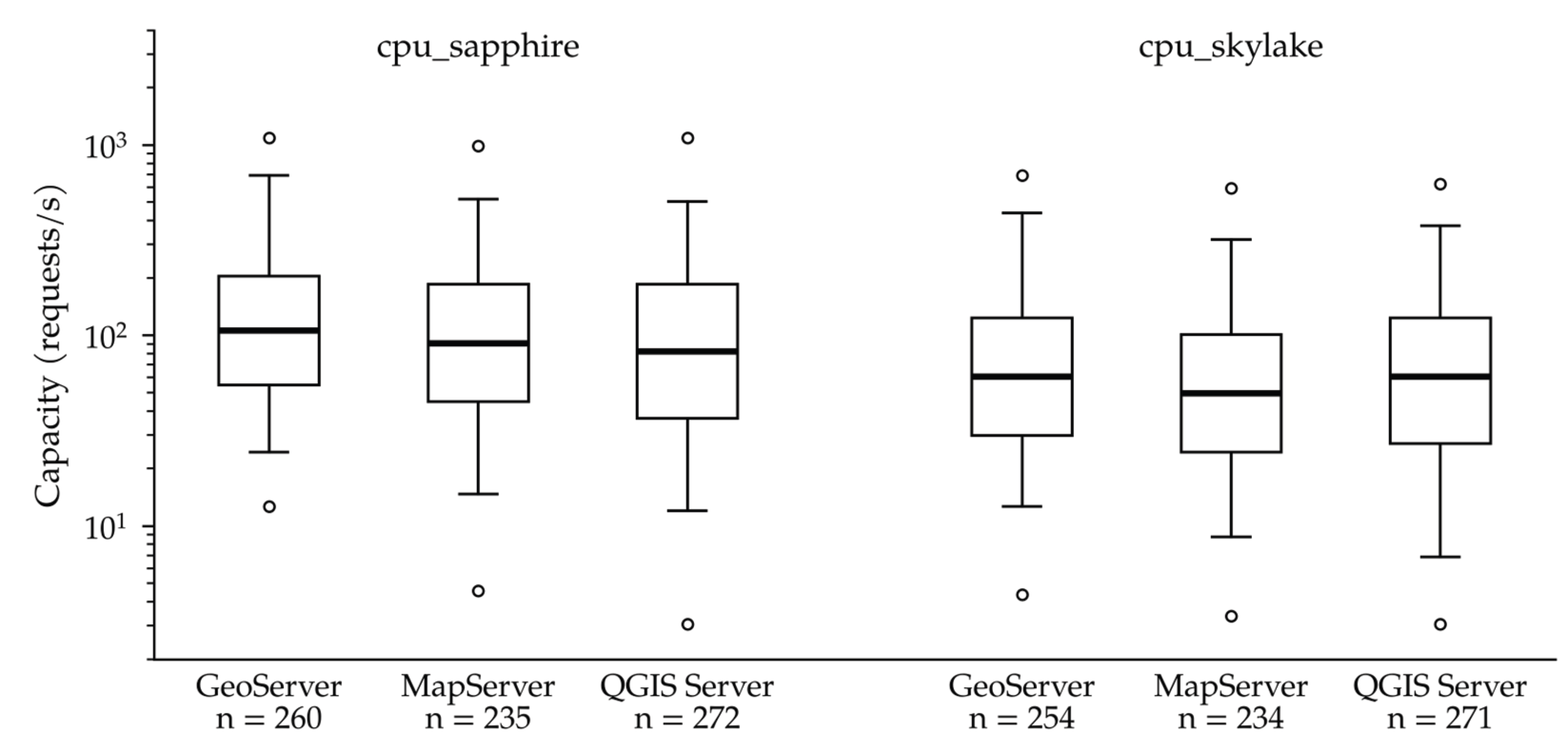
Figure 2.
Total-order Sobol indices for log capacity on cpu_sapphire: (a) pooled surrogate with the engine as an input; (b to d) each engine over its own factors. Lines: 95% bootstrap intervals.
Figure 2.
Total-order Sobol indices for log capacity on cpu_sapphire: (a) pooled surrogate with the engine as an input; (b to d) each engine over its own factors. Lines: 95% bootstrap intervals.
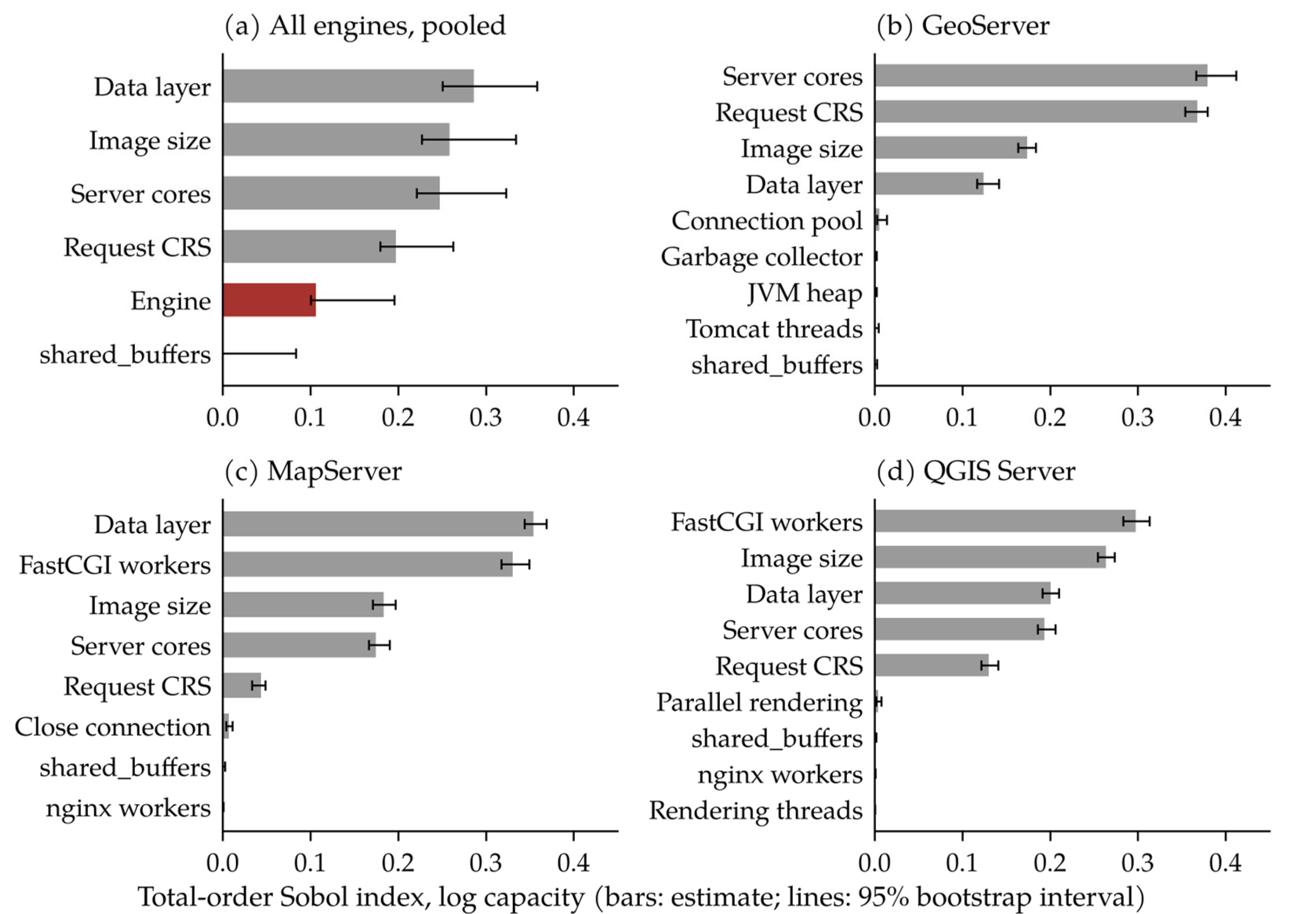
Figure 3.
Probability that the first engine is better (higher capacity, lower latency) over the factor space. Filled circles: cpu_sapphire with 95% bootstrap interval; open diamonds: cpu_skylake; squares: cpu_sapphire restricted to 2 and 10 km maps. Right column: reversal share of the common-factor cells on cpu_sapphire. GS: GeoServer; MS: MapServer; QGIS: QGIS Server.
Figure 3.
Probability that the first engine is better (higher capacity, lower latency) over the factor space. Filled circles: cpu_sapphire with 95% bootstrap interval; open diamonds: cpu_skylake; squares: cpu_sapphire restricted to 2 and 10 km maps. Right column: reversal share of the common-factor cells on cpu_sapphire. GS: GeoServer; MS: MapServer; QGIS: QGIS Server.
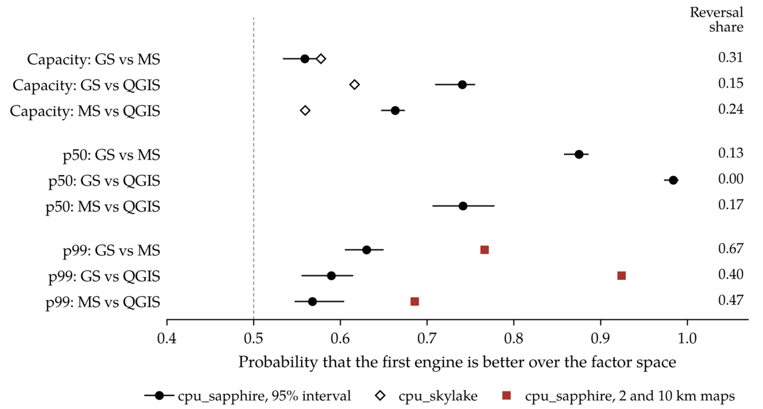
Figure 4.
Research question 3 (RQ3) at the reference workload (poly_v16, 512 px, EPSG:3035, 4 server cores), cpu_sapphire. Batch 0: main-batch sessions with a valid launch at this workload; BO: the configurations evaluated by Bayesian optimisation; Confirm: the three replicate jobs of each selected configuration. Each dot is a session at the midpoint of its knee bracket; grey lines mark the rates of the 1.5^(k/4) grid, so every bracket lies between two adjacent lines. Numbers give the sessions at each value; diamonds: confirmation jobs; red open circles: MapServer sessions without a valid launch (1 + 5: one valid session and five without a valid launch).
Figure 4.
Research question 3 (RQ3) at the reference workload (poly_v16, 512 px, EPSG:3035, 4 server cores), cpu_sapphire. Batch 0: main-batch sessions with a valid launch at this workload; BO: the configurations evaluated by Bayesian optimisation; Confirm: the three replicate jobs of each selected configuration. Each dot is a session at the midpoint of its knee bracket; grey lines mark the rates of the 1.5^(k/4) grid, so every bracket lies between two adjacent lines. Numbers give the sessions at each value; diamonds: confirmation jobs; red open circles: MapServer sessions without a valid launch (1 + 5: one valid session and five without a valid launch).
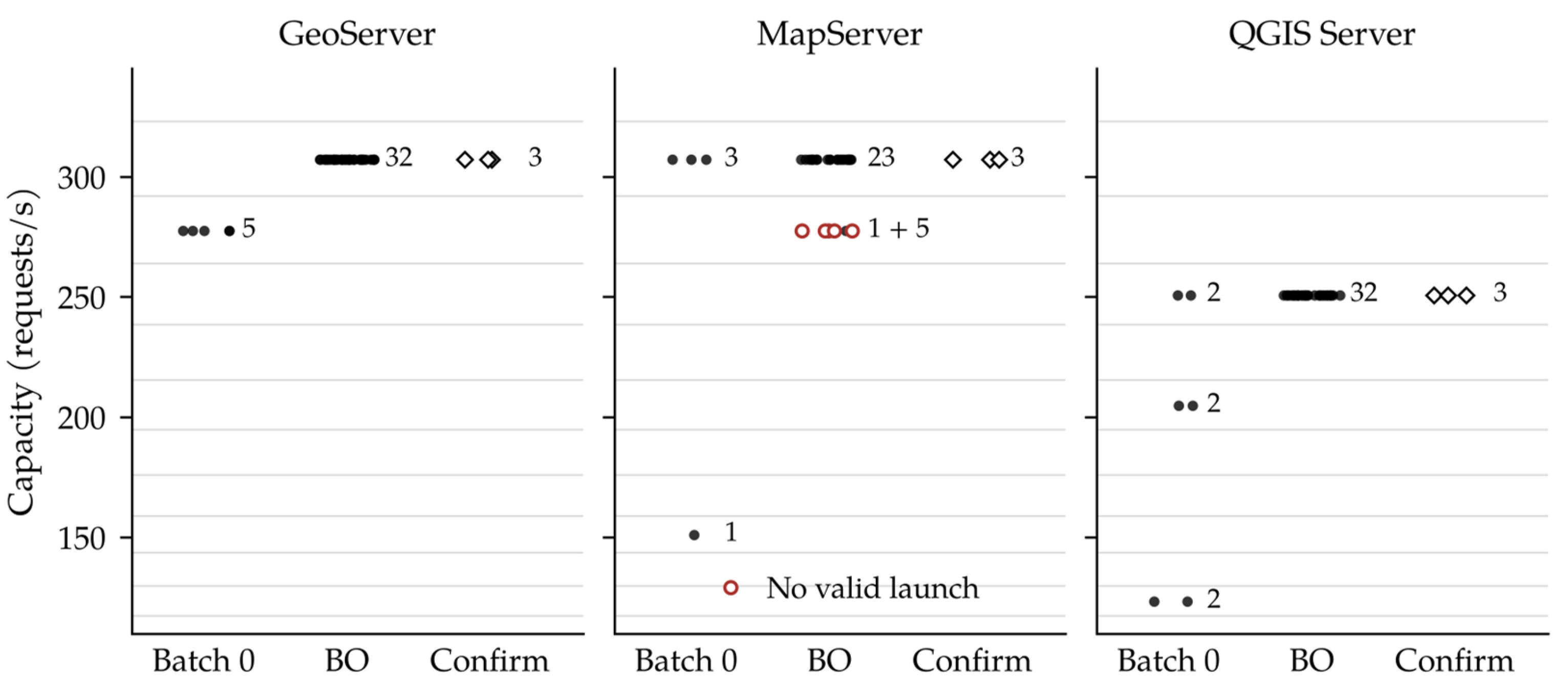
Figure 5.
Growth of (a) median latency and (b) 99th-percentile (p99) latency with offered load, relative to the median latency at the lowest level of each launch, cpu_sapphire. Lines: median over valid unsaturated levels in each bin; vertical bars: interquartile range of p99.
Figure 5.
Growth of (a) median latency and (b) 99th-percentile (p99) latency with offered load, relative to the median latency at the lowest level of each launch, cpu_sapphire. Lines: median over valid unsaturated levels in each bin; vertical bars: interquartile range of p99.
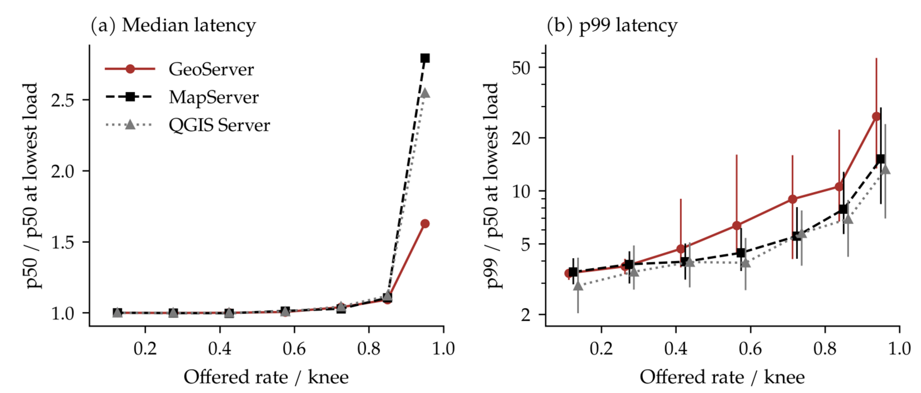
Table 1.
Server-specific factors (full ranges in the frozen factors.json).
| Server | Server-specific factors |
|---|---|
| GeoServer | JVM heap, garbage collector, Tomcat thread limit, connection pool size |
| MapServer | FastCGI workers (log-uniform, 1 to 64), connection handling, nginx workers |
| QGIS Server | FastCGI workers, rendering threads, parallel rendering, nginx workers |
Table 2.
Noise components on the anchor configurations (standard deviations on the log scale; restricted maximum likelihood (REML) with crossed random intercepts).
Table 2.
Noise components on the anchor configurations (standard deviations on the log scale; restricted maximum likelihood (REML) with crossed random intercepts).
| Platform, outcome | Node | Job | Launch | Launches |
|---|---|---|---|---|
| cpu_sapphire, log capacity | <0.001 | <0.001 | 0.044 | 138 |
| cpu_sapphire, log p50 (50% knee) | 0.004 | 0.009 | 0.014 | 122 |
| cpu_sapphire, log p99 (50% knee) | <0.001 | 0.020 | 0.021 | 122 |
| cpu_skylake, log capacity | 0.073 | 0.093 | 0.033 | 138 |
| cpu_skylake, log p50 (50% knee) | 0.073 | 0.109 | 0.015 | 124 |
| cpu_skylake, log p99 (50% knee) | 0.035 | 0.089 | 0.019 | 124 |
Table 3.
Total-order Sobol indices of the pooled surrogate (common factors and engine), cpu_sapphire, with 95% bootstrap intervals. Total-order indices include interactions and do not sum to one.
Table 3.
Total-order Sobol indices of the pooled surrogate (common factors and engine), cpu_sapphire, with 95% bootstrap intervals. Total-order indices include interactions and do not sum to one.
| Factor | log capacity | log p50 (50% knee) | log p99 (50% knee) |
|---|---|---|---|
| Engine | 0.11 (0.10-0.20) | 0.13 (0.13-0.16) | 0.11 (0.11-0.12) |
| Data layer | 0.29 (0.25-0.36) | 0.38 (0.36-0.40) | 0.42 (0.41-0.43) |
| Image size | 0.26 (0.23-0.33) | 0.49 (0.47-0.51) | 0.24 (0.23-0.25) |
| Server cores | 0.25 (0.22-0.32) | 0.00 (0.00-0.05) | 0.03 (0.03-0.04) |
| Request CRS | 0.20 (0.18-0.26) | 0.06 (0.06-0.10) | 0.36 (0.35-0.37) |
| shared_buffers | 0.00 (0.00-0.08) | 0.00 (0.00-0.02) | 0.00 (0.00-0.01) |
Table 4.
Probability that the first engine is better (higher capacity, lower latency) over the factor space, with the share of common-factor cells where the expected difference reverses. cpu_sapphire unless marked.
Table 4.
Probability that the first engine is better (higher capacity, lower latency) over the factor space, with the share of common-factor cells where the expected difference reverses. cpu_sapphire unless marked.
| Outcome | GeoServer vs MapServer | GeoServer vs QGIS Server | MapServer vs QGIS Server |
|---|---|---|---|
| Capacity | 0.56 (rev. 0.31) | 0.74 (rev. 0.15) | 0.66 (rev. 0.24) |
| Capacity, cpu_skylake | 0.58 (rev. 0.35) | 0.62 (rev. 0.36) | 0.56 (rev. 0.41) |
| p50 at 50% knee | 0.88 (rev. 0.13) | 0.98 (rev. 0.00) | 0.74 (rev. 0.17) |
| p99 at 50% knee | 0.63 (rev. 0.67) | 0.59 (rev. 0.40) | 0.57 (rev. 0.47) |
| p99, 2 and 10 km only | 0.77 (rev. 0.21) | 0.92 (rev. 0.02) | 0.69 (rev. 0.25) |
| p99/p50 ratio | 0.19 (rev. 0.08) | 0.10 (rev. 0.08) | 0.36 (rev. 0.41) |
Table 6.
Prediction of cpu_skylake sessions from cpu_sapphire surrogates: median absolute log error and coverage of the 95% prediction interval.
Table 6.
Prediction of cpu_skylake sessions from cpu_sapphire surrogates: median absolute log error and coverage of the 95% prediction interval.
| Engine, outcome | Raw error (coverage) | Calibrated error (coverage) | Sessions |
|---|---|---|---|
| GeoServer, log capacity | 0.58 (0.00) | 0.30 (0.14) | 254 |
| MapServer, log capacity | 0.59 (0.00) | 0.27 (0.06) | 234 |
| QGIS Server, log capacity | 0.42 (0.25) | 0.28 (0.18) | 271 |
| GeoServer, log p99 | 0.65 (0.01) | 0.37 (0.04) | 197 |
| MapServer, log p99 | 0.57 (0.01) | 0.26 (0.07) | 219 |
| QGIS Server, log p99 | 0.49 (0.11) | 0.37 (0.05) | 266 |
Disclaimer/Publisher’s Note: The statements, opinions and data contained in all publications are solely those of the individual author(s) and contributor(s) and not of MDPI and/or the editor(s). MDPI and/or the editor(s) disclaim responsibility for any injury to people or property resulting from any ideas, methods, instructions or products referred to in the content. |
© 2026 by the authors. Licensee MDPI, Basel, Switzerland. This article is an open access article distributed under the terms and conditions of the Creative Commons Attribution (CC BY) license (http://creativecommons.org/licenses/by/4.0/).
Copyright: This open access article is published under a Creative Commons CC BY 4.0 license, which permit the free download, distribution, and reuse, provided that the author and preprint are cited in any reuse.