

Submitted:
15 October 2026
Posted:
16 October 2026
You are already at the latest version
Abstract
Embedding the engines in the rear fuselage is a promising concept to reduce aircraft fuel consumption, but it leads to complex load paths and can introduce engine vibrations into the fuselage skin. Sandwich panels with an auxetic metamaterial core are a potential skin concept for this region, as they can be tailored locally and enhance energy dissipation and passive vibration damping. However, modeling the individual cells for a fuselage structure leads to infeasibly large system sizes. This work therefore presents a scale-bridging analysis framework that homogenizes sandwich materials with auxetic cores into shell stiffnesses for macroscale structural design. For this, a first-order computational homoge-nization of the core combined with classical laminate theory and an asymptotic homogenization of the complete sandwich section are considered. Both are compared against a reference model with a resolved core under tension, shear and bending as well as in a modal analysis, with deviations below 6% for the asymptotic homogenization. The homogenized stiffnesses are then used in an isogeometric analysis of a rear fuselage with embedded engines. Under a 2.5 g pull-up maneuver, the core topology and its orientation directly influence the global deformation, making the core topology a design variable at the aircraft scale.
Keywords:
sogeometric analysis
; auxetic metamaterials
; numerical homogenization
; sandwich composites
1. Introduction and Motivation
The aviation industry is under significant pressure to reduce its environmental impact. Boundary layer ingestion (BLI) is a promising way to reduce fuel consumption. By embedding the engines into the fuselage, the boundary layer forming on the fuselage is ingested into the engine, which re-energizes the aircraft’s wake. As a result, the wake drag is reduced and the overall efficiency is improved, with an expected energy saving of approximately 5–8% [2,3,4,5]. However, the engine inlet no longer receives a clean free stream but the distorted boundary layer of the fuselage, whose state changes considerably over the flight envelope and can provoke flow separation in different regions of the intake [6]. This could be addressed by morphing the engine inlet skin to adapt the aerodynamic surface for different flight conditions. Structurally, the skin around the inlet must carry the loads introduced by the embedded engines into the rear fuselage while limiting the transmission of engine vibrations and the resulting cabin noise.
A promising solution for these requirements is the use of auxetic metamaterials, which are engineered cellular structures with a negative Poisson’s ratio, where the cell geometry rather than the base material governs the deformation. Used as a sandwich core, such cells interact with the non-auxetic face sheets such that energy is stored and dissipated more effectively than in a conventional sandwich [7,8]. This behavior has been exploited for enhanced energy dissipation [9], high energy absorption [10] and passive vibration damping [11]. Since the response follows from the cell geometry, it can be tuned locally and very precisely through the deformation mechanism of the cell [12], without changing the base material.
In BLI configurations, such sandwiches with an auxetic core can offer favorable characteristics for the inlet region, as the face sheets provide a smooth surface to guide the flow while the tailored mechanical behavior is preserved beneath. Beyond this passive behavior, auxetic materials also open up the possibility of a morphing surface [13,14], which can offer significant advantages for the flow characteristics [15], and they provide stabilizing effects on curved and double-curved surfaces [16].
Despite these advantages, significant obstacles still prevent the widespread use of auxetic metamaterials in aerospace applications, one reason being the extensive numerical modeling effort. For components of the size of the proposed embedded engine inlet region, the complex cell geometry increases the system size considerably. The unit cells are smaller than the macroscopic component by orders of magnitude, making it prohibitively expensive to resolve their fine details. Many auxetic structures additionally feature notches, which further increase the modeling effort and the complexity. The resulting system size leads to high computational costs and makes it difficult to investigate real-world engineering problems.
Various approaches have been proposed to reduce the computational effort associated with such structures without compromising the accuracy required for analyzing the fine-scale properties described above. Notable examples include methods for reduced-fidelity modeling [17], several approaches involving machine learning [18], asymptotic homogenization [19] and two-scale computational homogenization [20]. These approaches differ mainly in their field of application. Reduced-fidelity modeling methods are applied to lattices with large auxetic cells, which allow for scale separation only to a limited extent, if at all, and therefore must retain a simplified representation of the cell geometry. Machine learning approaches, on the other hand, often involve inverse design or the generation of response surfaces that map the cell parameters to the effective properties by nonlinear interpolation and extrapolation, so that objective functions can be evaluated efficiently in areas such as structural optimization. Lastly, a wide variety of homogenization approaches are used to predict the overall behavior of large-scale structures with a clear separation of scales. Since the auxetic cells considered here are orders of magnitude smaller than the fuselage skin, the present work fits to this last category.
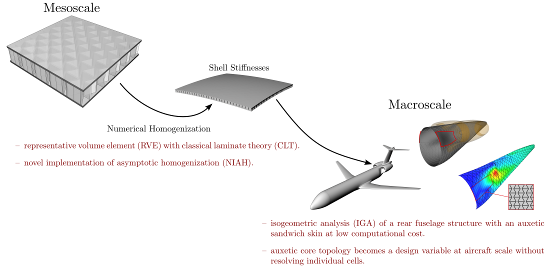
The novel contribution of this article is the homogenization of an auxetic-core sandwich, which makes the advantages listed above accessible while keeping the macroscale analysis computationally manageable. The framework is shown in Figure 1 and the two scales are described in Section 2. At the mesoscale, the ABD matrix of the auxetic sandwich section is obtained by numerical homogenization (Section 3). Two approaches are compared with a resolved reference model under tension, shear and bending as well as in a modal analysis (Section 4). At the macroscale, the rear fuselage is modeled with isogeometric analysis (IGA), which allows the structural analysis to be performed directly on the CAD description of the fuselage without a separate meshing step. The homogenized stiffness is then assigned to the skin of the inlet region, and the influence of the core topology and its orientation on the global deformation under a pull-up maneuver is evaluated (Section 5). This novel approach, combining the design of auxetic unit cells at the mesoscale with isogeometric analysis for the structural analysis at the macroscale, enables the core topology to be used as a design variable at the aircraft scale.
2. Scale-Bridging Analysis Framework
2.1. Mesoscale: Auxetic Sandwich
In this article, a re-entrant auxetic cell is chosen as the representative unit cell, as shown in Figure 2. Its geometry is deliberately simple, essentially being a honeycomb with inverted diagonal struts. This allows it to be adapted to existing components with little geometric effort, while still producing an auxetic effect resulting from the re-entrant angle of the diagonal struts. The corresponding dimensions are listed in Table 1, where w and h denote the total width and height of a cell, H the core height and t the strut thickness.
2.2. Macroscale: Structural Design Using Isogeometric Analysis
At the macroscale, the overall aim of the project is to identify unconventional stiffening topologies that minimize the structural weight of the rear fuselage using isogeometric analysis (IGA) [21]. IGA uses the same basis functions for the analysis that already describe the geometry, in this case non-uniform rational B-splines (NURBS). Geometry and simulation model are therefore no longer two separate representations. Instead, the CAD description of the outer fuselage shape is the analysis model itself, so that the meshing step and the geometric approximation it introduces are avoided [22]. Refinement reduces to knot insertion or degree elevation on that same description, which keeps the geometry exact at every refinement level and provides high solution accuracy with comparatively few degrees of freedom. Since the basis functions can be up to -continuous across element boundaries, element formulations with continuity requirements beyond become accessible. In this study, isogeometric Kirchhoff–Love shell elements are used, which require continuity and therefore cannot be formulated with classical -continuous Lagrange basis functions.
A further advantage of using IGA is the possibility of modeling the stiffeners as beams embedded into the fuselage shell, as proposed by Bauer et al. [23]. For the fuselage structural design, the stringer layouts are described as curves in the parameter space of the fuselage shell and mapped into physical space, so that the stiffeners introduce no degrees of freedom of their own. Instead, their structural response is expressed entirely through the shell. The stiffener layout is thereby decoupled from the shell discretization so that a stiffener can be moved, added or removed without remeshing. Together with the direct use of the CAD geometry, this makes the approach well suited for the early design stage, where the outer fuselage shape, the position of the embedded engines and the stiffening layout all change from one design variant to the next.
3. Homogenization Approaches
This section presents two different homogenization approaches that transfer the advantages of auxetic materials from the mesoscale (Section 2.1) to the macroscale (Section 2.2).
3.1. Computational Homogenization of a Periodic Unit Cell
The first approach consists of two steps, which are illustrated in Figure 3. First, the material properties of the auxetic sandwich core are determined on a unit cell acting as a representative volume element (RVE), using first-order computational homogenization. Second, the ABD matrix of the shell is calculated using classical laminate theory (CLT) by integrating the layer stiffnesses through the thickness.
3.1.1. Homogenization of the Sandwich Core Material
The goal of homogenization is to replace the periodic mesostructure, in this case the auxetic sandwich core structure, with an equivalent homogeneous medium that reflects the cell-averaged stiffness and deformation behavior. To this end, the displacement field of the unit cell is split into a linear macroscopic part and a periodic fluctuation, , where the fluctuation takes the same value at any two opposite boundary points. Since the cell walls are prismatic in the z-direction, the deformation under periodic boundary conditions is uniform along z, and the homogenized properties do not depend on the height of the RVE. To reduce the model size, a slice of height is therefore used instead of the full core height H. Opposite faces are separated by the period vectors , or in the x-, y- and z-directions (see Figure 4). Subtracting the displacements of such a boundary pair therefore cancels the fluctuation and leaves
Consequently, the relative displacement of every boundary pair is prescribed by the macroscopic strain tensor and the cell dimensions alone, independent of the position on the face. The three resulting offsets are assigned to the displacements of one reference point per direction, , and , and enforced by linear constraint equations between each dependent node d and its independent periodic image n on the opposite face. This leads to the following equations
with the reference-point displacements holding the columns of the macroscopic strain tensor scaled by the respective cell period,
The RVE is discretized with shell elements having rotational degrees of freedom. Therefore, the boundary rotations must be periodic as well. Since there is no macroscopic curvature in first-order homogenization, the rotational fluctuation is periodic and the jump disappears entirely. For the pairs of opposite faces, the constraints read
The green and blue edges in Figure 4 belong to two face pairs simultaneously, so nodes on these edges are paired in one direction only. Furthermore, one interior node is fixed to remove the rigid-body translation. To compute the material properties, three tension and three shear load cases are applied, which are listed in Table 2. The reaction force () at a reference point equals the resultant force transmitted across the corresponding cell face, and the areas of the RVE faces are , and .
Uniaxial tension in x is imposed by prescribing , which corresponds to a unit strain . The reference points and remain unloaded, and only their normal components and are left unconstrained (Table 2). As a result, the cell can deform freely in the transverse directions. The Young’s modulus and the Poisson’s ratios then follow from the effective stresses and the respective strains. For tension in the x-direction, the effective stresses and strains are
From these relations, the Young’s modulus and the two Poisson’s ratio components and can be calculated as follows:
Tension in y and z is applied in the same manner and yields , , , as well as , , . For the shear cases, the strain jump is introduced at two reference points simultaneously. For shear in the x–y plane, this leads to and . The shear stress is then available from either reference point,
The remaining shear moduli follow analogously as
3.1.2. Computation of the ABD Matrix
The homogenized core is now treated as one thick ply in the composite stack (see Figure 3). Its orthotropic constants are the RVE results computed in the previous section. The ABD matrices used for the isogeometric shell model are computed according to CLT [22], which was implemented in the IGA solver of Kratos Multiphysics [24]. For each layer k, the reduced plane-stress stiffness is computed as
The reduced plane-stress stiffness matrix is then rotated by the ply angle with the strain transformation matrix :
To compute the ABD matrices, the rotated matrices are integrated over the through-thickness coordinates of the layer boundaries, measured from the laminate midplane:
Although the approach is simple to implement, it is based on assumptions that the real sandwich does not satisfy. First, the continuum assumption requires the cell to be small compared to the region it fills. In plane, this can be achieved with sufficiently small cells. Through the thickness, however, the core height H is of the same order as the cell dimensions and the core is bounded by the face sheets, whereas the periodic constraints in z treat it as an infinitely extended medium. Second, classical laminate theory reduces every layer to a plane stress state, so that only , , and enter the reduced stiffness , while , , , and are discarded. An alternative approach to calculating the ABD matrix that avoids these problems is asymptotic homogenization, which is described in the next section.
3.2. Asymptotic Homogenization
The second approach is based on the NIAH (Novel Implementation of Asymptotic Homogenization) method [25,26], which originates from the homogenization theory of plates with in-plane periodic microstructure, developed by Kalamkarov et al. [19]. Like the first approach, it requires only standard FE solutions. However, it homogenizes the complete periodic sandwich section (auxetic core and both face laminates), which directly results in the ABD matrix without an intermediate core material (see Figure 5).
The idea of asymptotic homogenization of periodic plate structures is based on defining a periodic unit cell whose thickness and in-plane dimensions are small compared to the dimensions of the component. The stresses and displacements are then expressed through an asymptotic expansion, which leads to equilibrium equations for the unit cell under in-plane periodic boundary conditions. These equations can be solved analytically or by transforming the problem into a finite element formulation, which, however, requires access to the internal structure of the FE solver.
The idea of NIAH is to circumvent this by expressing every step as a standard static solve of a commercial code [25,26]. First, a finite element model of the unit cell is constructed. Then, for each of the six unit macroscopic states (three membrane strains and three curvatures) the corresponding nodal displacement field is applied to every node of the unconstrained unit cell. The reaction force vectors for this nodal field can then be computed as . These forces are then applied to the unit cell with in-plane periodic constraints and free top and bottom surfaces, yielding the characteristic displacements of every node. In a third solve, the characteristic displacements are applied to the unconstrained cell, which returns the nodal reaction forces and allows for the computation of the effective material properties, which are the entries of the ABD matrix [26].
The original method is restricted to elements with translational degrees of freedom. Recently, Liu et al. developed an Abaqus plug-in that also allows the use of elements with rotational degrees of freedom [27]. This makes it directly applicable to the present cell meshed with S4 shell elements. The plug-in requires a unit cell that is mirror-symmetric about the coordinate axes, with the nodes on opposite boundary faces matching one to one. The shared cell walls in the x–z plane were therefore split into two halves along the cell end faces, one belonging to each neighboring cell. Each half is a shell of thickness whose nodes lie on the cell face and whose section is offset by half of its own thickness toward the cell interior (see Figure 6). Since the plug-in enforces periodicity for all six degrees of freedom of the boundary nodes, the two halves deform as one continuous wall.
3.3. Homogenization of the Mass
The modal analysis in Section 4 additionally requires the inertia of the section. Unlike for the stiffness, no cell problem has to be solved, since the kinetic energy is a plain volume average. The effective core density is the density of the wall material scaled by the relative density of the cell, , and the core is treated as an additional homogeneous layer of the section. The relevant quantity for a shell is the mass per unit area,
where the density is integrated along the thickness coordinate z, which reduces to the sum of thickness times density over the layers k of the section, i.e., the two face laminates with thickness and density and the homogenized core with height H and density . For the symmetric section the first moment vanishes, and rotary inertia is neglected. Hence, is the only inertia term of the thin-shell model.
4. Comparison at the Panel Level
4.1. Comparison of the ABD Matrices
First, the ABD matrices resulting from the two homogenization approaches of Section 3.1 and Section 3.2 are compared. For all comparisons below, the auxetic unit cell measures mm in plane, with a height of mm, a wall thickness of mm and a re-entrant angle of (see Figure 2). A stainless spring steel (EN 1.4310) with MPa, and g/cm3 is used as the auxetic core material.
The face laminates are quasi-isotropic layups with a ply thickness of mm, which gives a thickness of mm per face. The ply is oriented along the x-axis of the auxetic cell, which coincides with the x-axis of the panel in the examples below. An S2-glass/epoxy with MPa, MPa, , MPa and g/cm3 is used for the plies ([28] [Table 1]).
For the homogenized auxetic core, the method of Section 3.1 yields MPa, MPa, MPa, and . The reduced plane-stress stiffness computed from these constants with Equation (9) is then inserted into the CLT routine of the IGA code as an additional core layer between the two face laminates, which results in a stack of 17 layers. The ABD matrix that follows from Equation (11) is shown on the left in Figure 7, next to the matrix obtained with the asymptotic homogenization of Section 3.2 on the right. The entries of are given in MN/m and those of in N m. The color of each block is scaled by its maximum absolute value with the same scale used for both approaches.
To isolate the core contribution, the face-laminate contribution (Equation (11)) is subtracted from both ABD matrices (Figure 8).
A comparison of the two core contributions shows that the first-order homogenization yields the more compliant core, with being approximately lower than the NIAH result. At the same time, it indicates a more pronounced auxetic response under in-plane loading, since is about larger in magnitude. Next, both homogenized models are compared with the resolved model under different load cases.
4.2. Square Plate Under Different Load Cases
4.2.1. Axial Tension
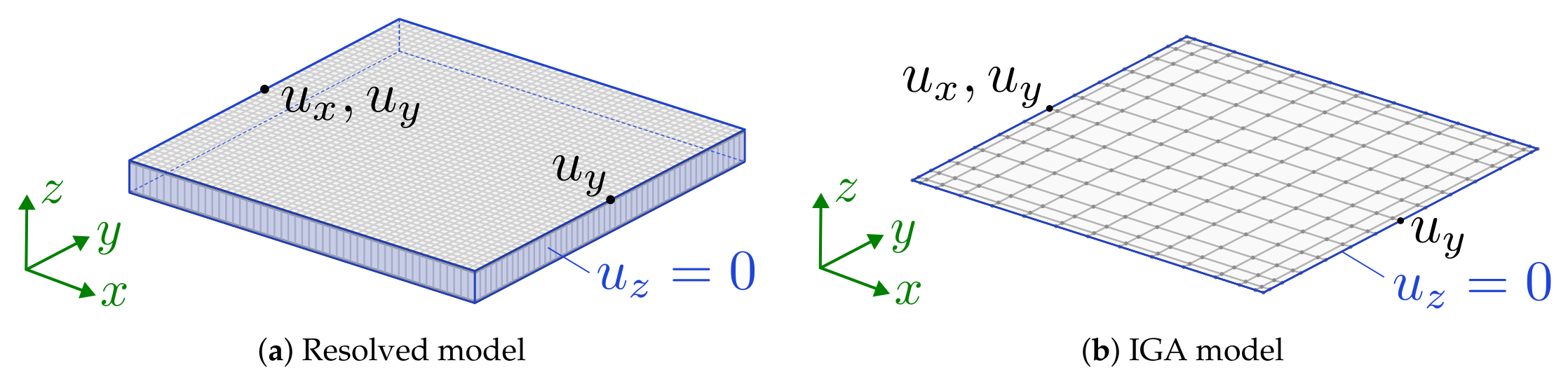
As a first example, a mm plate under a uniaxial tension of N/mm is considered. The resolved model is analyzed with Abaqus using S4 shell elements and degrees of freedom. Figure A1(a) in Appendix A shows the boundary conditions of the resolved model. The axial resultant is introduced as a force of kN on a reference point that is tied to all nodes of the loaded end cross-section by linear constraint equations, so that this end remains plane. The opposite end is tied to a second reference point held at . Additionally, three pins on the outer face remove the remaining rigid-body motion.
The homogenized models are analyzed with Kratos Multiphysics using isogeometric Kirchhoff–Love shell elements with three translational degrees of freedom per control point. The mesh of control points results in 75 degrees of freedom. As shown in Figure A1(b), the IGA model introduces the same resultant as a line load on the control-point row at one end and keeps the ends plane by multi-point constraints. One point on the edge opposite the loaded edge is constrained in all three translations, and two further points are constrained in the z-direction to remove the remaining rigid-body motion.
Figure 9 shows the displacement field on the top surface of the resolved plate (a), compared with the IGA results obtained with the ABD matrix from the first-order computational homogenization (b) and from the asymptotic homogenization (c). The field deviations are shown in Figure A5 in Appendix B. As anticipated from the ABD matrix comparison, the asymptotic homogenization leads to smaller deviations, while the first-order homogenization is too compliant and overestimates the auxetic behavior. The same is observed in the comparison of the axial and lateral strains in Table 3, where the effective strains are evaluated from the edge-averaged displacements as
with the plate edge lengths mm.
4.2.2. In-Plane Shear
For the comparison under shear load, both models suppress the out-of-plane displacement along all four edges, and two corner points are pinned in plane to remove the remaining rigid-body motion (see Figure A2). The shear resultant of N/mm is applied as a tangential edge load q that forms a closed shear flow around the four edges, so that the load is self-equilibrated and each edge carries a total force of kN.
Figure 10 shows the displacement field of the resolved plate (a), compared with the IGA results obtained with the ABD matrix from the first-order computational homogenization (b) and from the asymptotic homogenization (c). The field deviations are shown in Figure A6 in Appendix B. As already seen for the axial case, the first-order homogenization is too compliant, while the asymptotic homogenization matches the resolved response closely. The effective shear strain in Table 4 is evaluated as a pair of central differences between the four mid-edge points of the plate, denoted by the superscripts , , and for the top, bottom, left and right mid-edge points,
so that the two terms of are the discrete counterparts of and . For both IGA models, the effective shear stiffness matches the entry of the corresponding ABD matrix in Figure 7.
4.2.3. Pure Bending
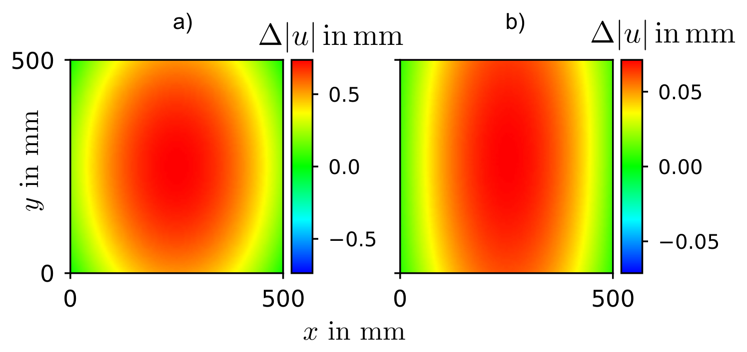
Pure bending is applied to the free plate with equal and opposite moments of N mm at the two ends, and three corner pins on the outer face remove rigid-body motion in both models (see Figure A3). In the resolved model, all nodes of each end face are coupled to a reference point that carries the moment. Since the Kirchhoff–Love shells of the IGA model have no rotational degrees of freedom, the same moment is introduced there as work-conjugate nodal loads on the control points of each end row.
Figure 11 shows the displacement field of the resolved plate (a), compared with the IGA results obtained with the ABD matrix from the first-order computational homogenization (b) and from the asymptotic homogenization (c). The field deviations are shown in Figure A7 in Appendix B. The curvatures in Table 5 are obtained by fitting a paraboloid to the out-of-plane displacement field by least squares, and the bending Poisson’s ratio follows as . Since the lateral edges are moment-free, equals the ratio of the corresponding ABD matrix in Figure 7. The first-order homogenization is again too compliant, overestimating by and underestimating by , while the asymptotic homogenization stays within of the resolved values.
4.2.4. Modal Analysis
For the modal analysis, the plate is simply supported along all edges, with two points pinned in plane to remove the remaining rigid-body motion (see Figure A4). Since the coarse control-point mesh of the static cases cannot represent the higher mode shapes, the discretization of the IGA models is refined for the modal analysis, resulting in the 1200 degrees of freedom listed in Table 6. Figure 12 compares the first four bending mode shapes and Table 6 the corresponding frequencies. Mode 2 of the resolved model is an in-plane mode and is omitted. All mode pairs reach a modal assurance criterion of , which rates the similarity of two mode shapes from 0 (no correspondence) to 1 (identical shapes), so that both homogenized models reproduce the mode shapes of the resolved plate. The first-order homogenization is again too compliant and therefore underestimates the frequencies by up to , while the asymptotic homogenization stays within . Since the asymptotic homogenization reproduces the resolved plate in all four comparisons, it is used for the fuselage analysis in Section 5.
5. Application to the Rear Fuselage Structure
The previous section has shown that shell stiffnesses homogenized using NIAH yield reliable results. This approach is now applied to the structural analysis of a rear fuselage with embedded engines. To this end, part of the stiffened outer skin near the embedded engine inlet is replaced by the homogenized auxetic sandwich material (marked in red in Figure 13).
Figure 14 shows the effect of the core topology and of its orientation within the patch on the deformation of the rear fuselage for a pull-up maneuver at ultimate load. Figure 14 illustrates the displacement field for the auxetic sandwich core material introduced earlier (see Figure 2). With the approach proposed above, it is now possible to change the core topology, repeat the homogenization and apply the updated sandwich properties to the skin area. Three variants are compared with the reference: the reference cell rotated by within the patch, and re-entrant angles of and , the latter corresponding to a conventional, non-auxetic honeycomb. Figure 14Figure 14 show the relative deviation of the displacement magnitude in percent with respect to the reference core topology in Figure 14. The core topology thus directly influences the global behavior of the rear fuselage. This opens up the possibility of optimizing the rear fuselage at both scales: at the macroscale by adapting the stiffener layout and at the mesoscale by adapting the sandwich core topology.
6. Summary and Outlook
The aim of this work was to lay the foundation for using auxetic metamaterials as the core of sandwich structures in order to exploit their advantages, such as passive vibration damping, high energy dissipation and tailorable deformation behavior. This could be particularly beneficial for the integration of engines into the fuselage for BLI configurations. However, a resolved simulation of the sandwich material is not feasible in this context.
Two homogenization approaches were investigated to determine the homogenized shell stiffnesses of auxetic sandwich materials. The first combines a first-order homogenization of the core, which is then treated as a laminate layer, with classical laminate theory to obtain the ABD matrix. The second approach is based on asymptotic homogenization. The resolved plate model and the two homogenized models were compared under tension, shear and bending as well as in a modal analysis. The asymptotic homogenization deviates from the resolved model by less than , while the first-order homogenization predicts an overly compliant response and is therefore not suitable for the macroscale analysis. The homogenized shell stiffnesses can now be used to perform the global structural simulations directly on the CAD geometry with few degrees of freedom using isogeometric analysis. This was demonstrated on a rear fuselage with embedded engines, where the stiffened skin of the inlet region was replaced by the homogenized sandwich material. Varying the core topology and its orientation showed a direct influence on the global deformation of the rear fuselage under a pull-up maneuver.
In the future, the homogenized transverse shear stiffnesses will also be determined, so that a shear-deformable shell theory can be used, which is particularly important for thick sandwich structures. Furthermore, these methods will be used for a simultaneous optimization of the stiffener topology at the macroscale and the auxetic core topology at the mesoscale.
Supplementary Materials
The following supporting information can be downloaded at the website of this paper posted on Preprints.org.
Author Contributions
Conceptualization, M.F.-D. and N.G.; methodology, M.F.-D. and N.G.; software, M.F.-D.; validation, M.F.-D.; investigation, M.F.-D. and N.G.; writing—original draft preparation, M.F.-D. and N.G.; writing—review and editing, S.K., M.H. and T.R.; visualization, M.F.-D.; supervision, S.K., M.H., T.R. and S.H.; project administration, M.H. and T.R.; funding acquisition, M.H. and T.R. All authors have read and agreed to the published version of the manuscript.
Funding
This work was funded by the Deutsche Forschungsgemeinschaft (DFG, German Research Foundation) – Project-ID 498601949 – TRR 364 (SynTrac, Project B06).
Data Availability Statement
The data supporting the findings of this study are available from the corresponding author upon request.
Conflicts of Interest
The authors declare no conflicts of interest. The funders had no role in the design of the study; in the collection, analyses, or interpretation of data; in the writing of the manuscript; or in the decision to publish the results.
Abbreviations
The following abbreviations are used in this manuscript:
| BLI | Boundary Layer Ingestion |
| CAD | Computer-Aided Design |
| CLT | Classical Laminate Theory |
| DOF | Degree of Freedom |
| FE | Finite Element |
| IGA | Isogeometric Analysis |
| MAC | Modal Assurance Criterion |
| NIAH | Novel Implementation of Asymptotic Homogenization |
| NURBS | Non-Uniform Rational B-Splines |
| RVE | Representative Volume Element |
Appendix A. Setup of the Plate Models
The load introduction and the boundary conditions of the resolved and the IGA plate models of Section 4 are sketched in Figure A1, Figure A2,Figure A3 and Figure A4.
Figure A1.
Load introduction and boundary conditions of the resolved model (a) and the IGA model (b) for the axial tension case.
Figure A1.
Load introduction and boundary conditions of the resolved model (a) and the IGA model (b) for the axial tension case.
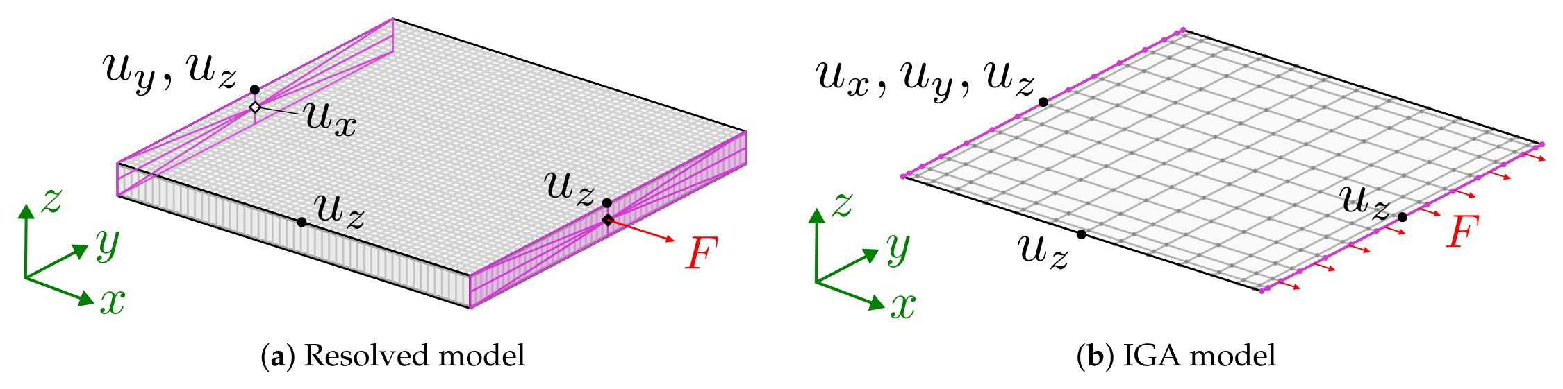
Figure A2.
Load introduction and boundary conditions of the resolved model (a) and the IGA model (b) for the shear case.
Figure A2.
Load introduction and boundary conditions of the resolved model (a) and the IGA model (b) for the shear case.
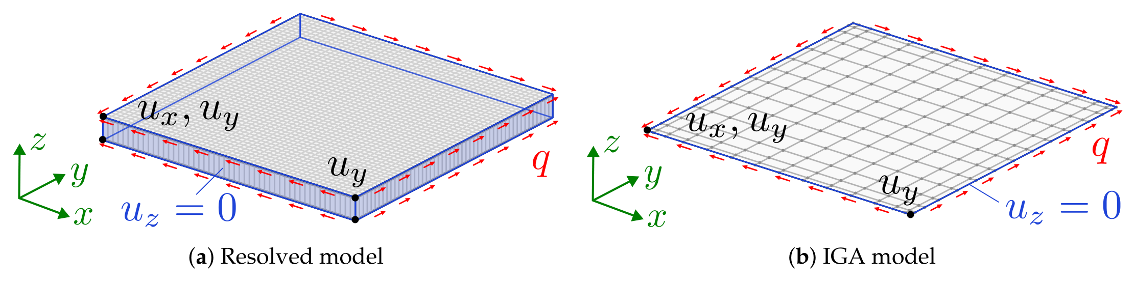
Figure A3.
Load introduction and boundary conditions of the resolved model (a) and the IGA model (b) for the bending case.
Figure A3.
Load introduction and boundary conditions of the resolved model (a) and the IGA model (b) for the bending case.
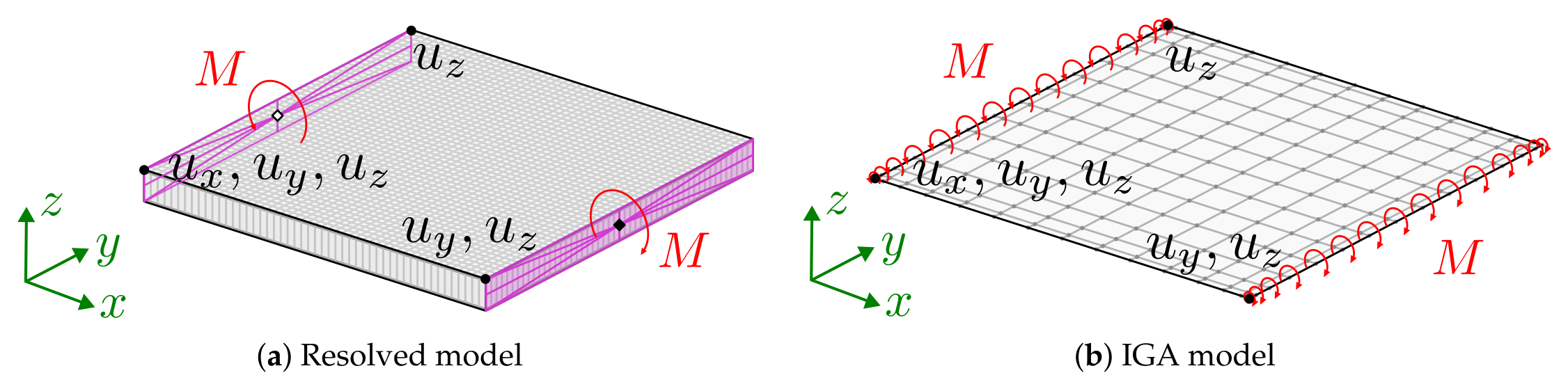
Figure A4.
Boundary conditions of the resolved model (a) and the IGA model (b) for the modal analysis.
Figure A4.
Boundary conditions of the resolved model (a) and the IGA model (b) for the modal analysis.
Appendix B. Deviation of the Displacement Fields
Figure A5.
Deviation of the displacement magnitude from the resolved plate model for the first-order computational homogenization (a) and the asymptotic homogenization (b) under axial tension.
Figure A5.
Deviation of the displacement magnitude from the resolved plate model for the first-order computational homogenization (a) and the asymptotic homogenization (b) under axial tension.
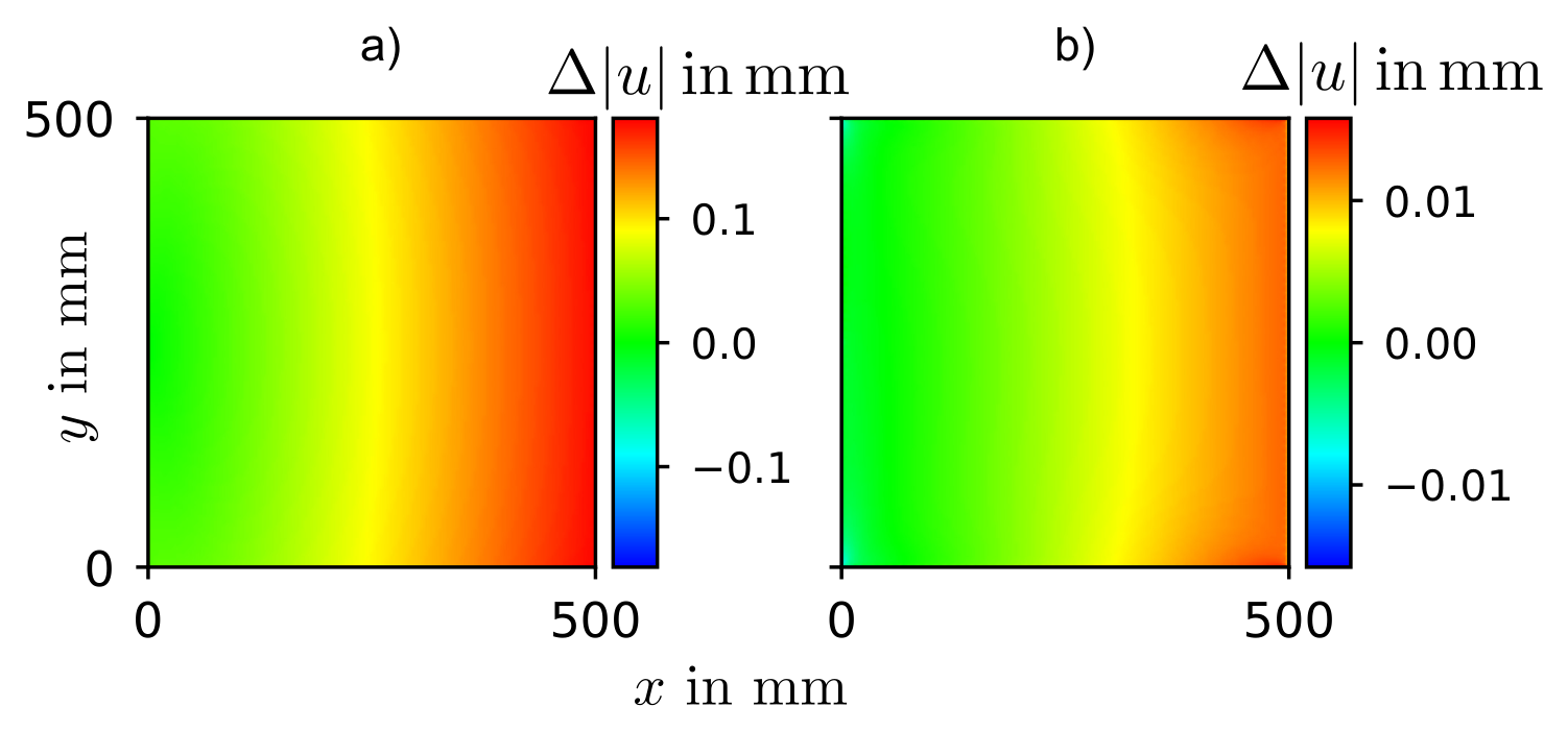
Figure A6.
Deviation of the displacement magnitude from the resolved plate model for the first-order computational homogenization (a) and the asymptotic homogenization (b) under shear.
Figure A6.
Deviation of the displacement magnitude from the resolved plate model for the first-order computational homogenization (a) and the asymptotic homogenization (b) under shear.
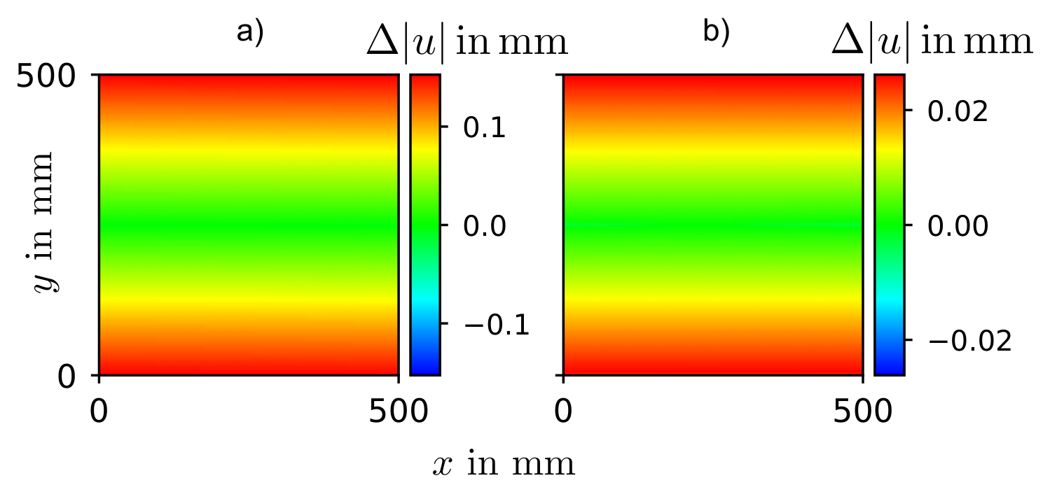
Figure A7.
Deviation of the displacement magnitude from the resolved plate model for the first-order computational homogenization (a) and the asymptotic homogenization (b) under bending.
Figure A7.
Deviation of the displacement magnitude from the resolved plate model for the first-order computational homogenization (a) and the asymptotic homogenization (b) under bending.
References
- Friedrichs-Dachale, M.; Grünfelder, N.; Haupt, M.; Kakkar, S.; Ricken, T.; Heimbs, S. A Scale-Bridging Analysis Framework for an Aircraft Rear Fuselage Structure with Integrated Engines Using Isogeometric Analysis and Auxetic Sandwich Composites. In Proceedings of the Proceedings of the Deutscher Luft- und Raumfahrtkongress 2026 (DLRK 2026), Aachen, Germany, 8–10 September 2026, 2026. in press. [Google Scholar]
- Vinz, A.; Raichle, A. Investigation of the effects of boundary layer ingestion engine integration on aircraft thrust requirement. CEAS Aeronaut. J. 2024, 15, 1235–1250. [Google Scholar] [CrossRef]
- Moirou, N.G.M.; Sanders, D.S.; Laskaridis, P. Advancements and prospects of boundary layer ingestion propulsion concepts. Prog. Aerosp. Sci. 2023, 138, 100897. [Google Scholar] [CrossRef]
- Uranga, A.; Drela, M.; Greitzer, E.M.; Hall, D.K.; Titchener, N.A.; Lieu, M.K.; Siu, N.M.; Casses, C.; Huang, A.C.; Gatlin, G.M.; et al. Boundary layer ingestion benefit of the D8 transport aircraft. AIAA J. 2017, 55, 3693–3708. [Google Scholar] [CrossRef]
- Pandya, S.A.; Uranga, A.; Espitia, A.; Huang, A. Computational assessment of the boundary layer ingesting nacelle design of the D8 aircraft. In Proceedings of the 52nd AIAA Aerospace Sciences Meeting AIAA Paper, National Harbor, MD, USA, January 2014; pp. 2014–0907. [Google Scholar] [CrossRef]
- Hartmann, J.; Staudacher, S. Engine-airframe integration — from Froude theorem to numerical flow simulation. Eng. Proc. 2026, 133, 151. [Google Scholar] [CrossRef]
- Qu, Y.C.; Teng, X.C.; Zhang, Y.; Jiang, W.Z.; Xue, M.L.; Xue, T.; Shi, J.W.; Ren, X. A novel 3D composite auxetic sandwich panel for energy absorption improvement. Eng. Struct. 2025, 322, 119129. [Google Scholar] [CrossRef]
- Liu, J.S.; Zhang, Y.; Wei, X.J.; Mi, Z.K.; Ding, T.; Zhang, J.H.; Cheng, T.; Hua, L.; Guo, X.; Lin, K.H.; et al. Four-point bending behavior of auxetic sandwich structures. Thin-Walled Struct. 2026, 227, 114954. [Google Scholar] [CrossRef]
- Boldrin, L.; Hummel, S.; Scarpa, F.; Di Maio, D.; Lira, C.; Ruzzene, M.; Remillat, C.D.L.; Lim, T.C.; Rajasekaran, R.; Patsias, S. Dynamic behaviour of auxetic gradient composite hexagonal honeycombs. Compos. Struct. 2016, 149, 114–124. [Google Scholar] [CrossRef]
- Francisco, M.B.; Pereira, J.L.J.; Oliver, G.A.; Roque da Silva, L.R.; Cunha, S.S., Jr.; Gomes, G.F. A review on the energy absorption response and structural applications of auxetic structures. Mech. Adv. Mater. Struct. 2022, 29, 5823–5842. [Google Scholar] [CrossRef]
- Grünfelder, N.; Brodbeck, M.; Waschinsky, N.; Ricken, T.; Seyedpour, S.M. Puzzle-like auxetic lattice architectures employing dovetail joints: Experimental investigation of the structural dynamic behaviour. Mater. Des. 2026, 268, 116408. [Google Scholar] [CrossRef]
- Nežerka, V.; Somr, M.; Janda, T.; Vorel, J.; Doškář, M.; Antoš, J.; Zeman, J.; Novák, J. A jigsaw puzzle metamaterial concept. Compos. Struct. 2018, 202, 1275–1279. [Google Scholar] [CrossRef]
- Hayashi, K.; Mesnil, R. Multi-layer auxetic surfaces with compliant mechanisms. Eng. Struct. 2025, 341, 120752. [Google Scholar] [CrossRef]
- Vocke, R.D.; Kothera, C.S.; Woods, B.K.S.; Wereley, N.M. Development and testing of a span-extending morphing wing. J. Intell. Mater. Syst. Struct. 2011, 22, 879–890. [Google Scholar] [CrossRef]
- Kling, U.; Seitz, A.; Bijewitz, J.; Hermanutz, A.; da Rocha-Schmidt, L.; Scarpa, F.; Majić, F.; Efraimsson, G.; O’Reilly, C.J. Shape adaptive technology for aircraft engine nacelle inlets. In Proceedings of the 5th Aircraft Structural Design Conference, Manchester, UK, October 2016; Royal Aeronautical Society. [Google Scholar]
- Pattinson, S.W.; Huber, M.E.; Kim, S.; Lee, J.; Grunsfeld, S.; Roberts, R.; Dreifus, G.; Meier, C.; Liu, L.; Hogan, N.; et al. Additive manufacturing of biomechanically tailored meshes for compliant wearable and implantable devices. Adv. Funct. Mater. 2019, 29, 1901815. [Google Scholar] [CrossRef]
- Grünfelder, N.; Padhy, M.; Armiti-Juber, A.; Seyedpour, S.M.; Waschinsky, N.; Ricken, T. Reduced-order modeling of lattice structures through iterative beam fitting and static mesoscale projection. Results Eng. 2025, 27, 106529. [Google Scholar] [CrossRef]
- Zhang, C.; Zhao, Y.F. A critical review on the application of machine learning in supporting auxetic metamaterial design. J. Phys. Mater. 2024, 7, 022004. [Google Scholar] [CrossRef]
- Kalamkarov, A.L.; Andrianov, I.V.; Danishevs’kyy, V.V. Asymptotic homogenization of composite materials and structures. Appl. Mech. Rev. 2009, 62, 030802. [Google Scholar] [CrossRef]
- Desmoulins, A.; Kochmann, D.M. Local and nonlocal continuum modeling of inelastic periodic networks applied to stretching-dominated trusses. Comput. Methods Appl. Mech. Eng. 2017, 313, 85–105. [Google Scholar] [CrossRef]
- Cottrell, J.A.; Hughes, T.J.R.; Bazilevs, Y. Isogeometric Analysis: Toward Integration of CAD and FEA; Wiley: Chichester, UK, 2009. [Google Scholar] [CrossRef]
- Sommerwerk, K. Isogeometrische Analyse für die Optimierung von Leichtbaustrukturen im Flugzeugbau. PhD thesis, Technische Universität Braunschweig, Braunschweig, Germany, 2017. [Google Scholar]
- Bauer, A.M.; Breitenberger, M.; Philipp, B.; Wüchner, R.; Bletzinger, K.U. Embedded structural entities in NURBS-based isogeometric analysis. Comput. Methods Appl. Mech. Eng. 2017, 325, 198–218. [Google Scholar] [CrossRef]
- Dadvand, P.; Rossi, R.; Oñate, E. An object-oriented environment for developing finite element codes for multi-disciplinary applications. Arch. Comput. Methods Eng. 2010, 17, 253–297. [Google Scholar] [CrossRef]
- Cheng, G.D.; Cai, Y.W.; Xu, L. Novel implementation of homogenization method to predict effective properties of periodic materials. Acta Mech. Sin. 2013, 29, 550–556. [Google Scholar] [CrossRef]
- Cai, Y.; Xu, L.; Cheng, G. Novel numerical implementation of asymptotic homogenization method for periodic plate structures. Int. J. Solids Struct. 2014, 51, 284–292. [Google Scholar] [CrossRef]
- Liu, Z.; Nie, Y.; Niu, B. A unified computational framework for asymptotic homogenization of periodic microstructures: 3D and Reissner–Mindlin plate numerical implementations. Compos. Struct. 2026, 396, 120827. [Google Scholar] [CrossRef]
- Kaddour, A.S.; Hinton, M.J. Input data for test cases used in benchmarking triaxial failure theories of composites. J. Compos. Mater. 2012, 46, 2295–2312. [Google Scholar] [CrossRef]
Figure 1.
Overview of the proposed scale-bridging analysis framework.
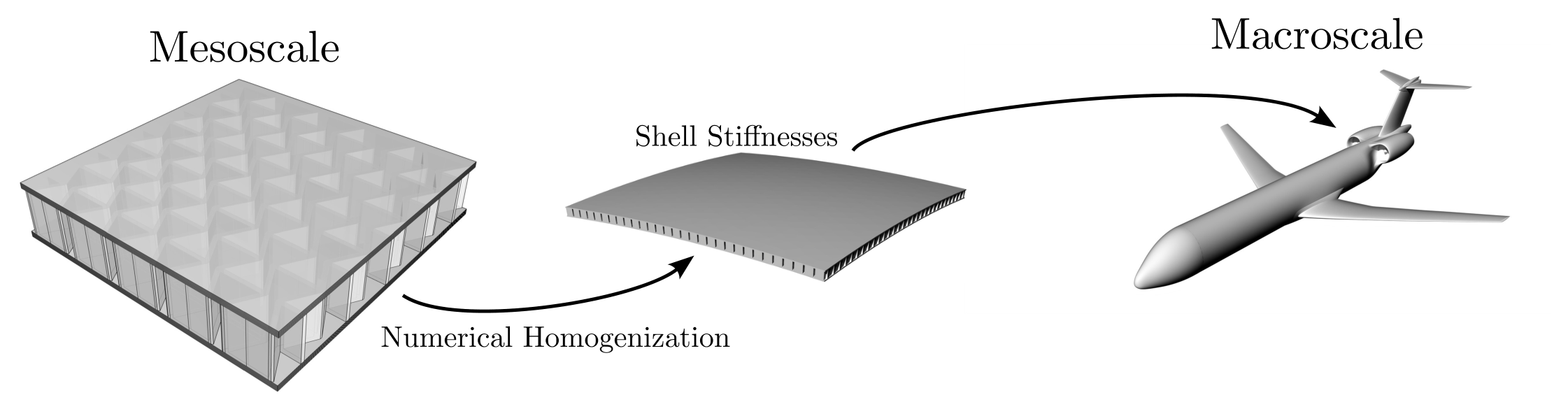
Figure 2.
Auxetic core dimensions and composite layout.
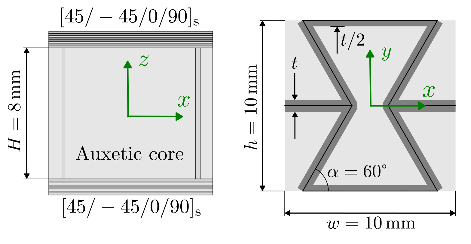
Figure 3.
Overview of the homogenization approach combining a representative volume element (RVE) with classical laminate theory (CLT), denoted CLT-RVE.
Figure 3.
Overview of the homogenization approach combining a representative volume element (RVE) with classical laminate theory (CLT), denoted CLT-RVE.
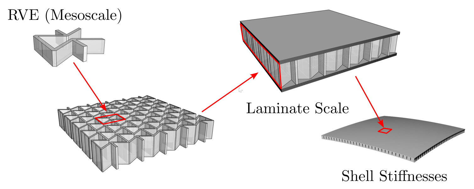
Figure 4.
Application of the periodic boundary conditions for the RVE.
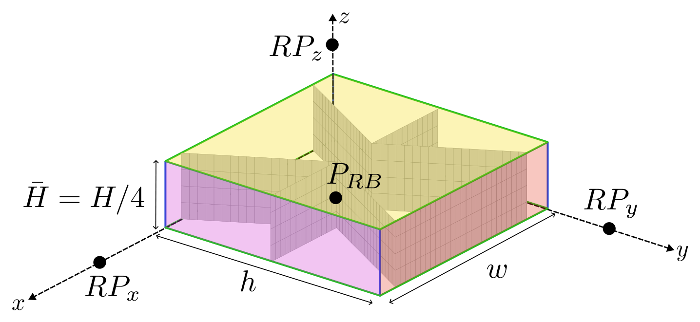
Figure 5.
Overview of the approach using the novel implementation of asymptotic homogenization (NIAH).
Figure 5.
Overview of the approach using the novel implementation of asymptotic homogenization (NIAH).
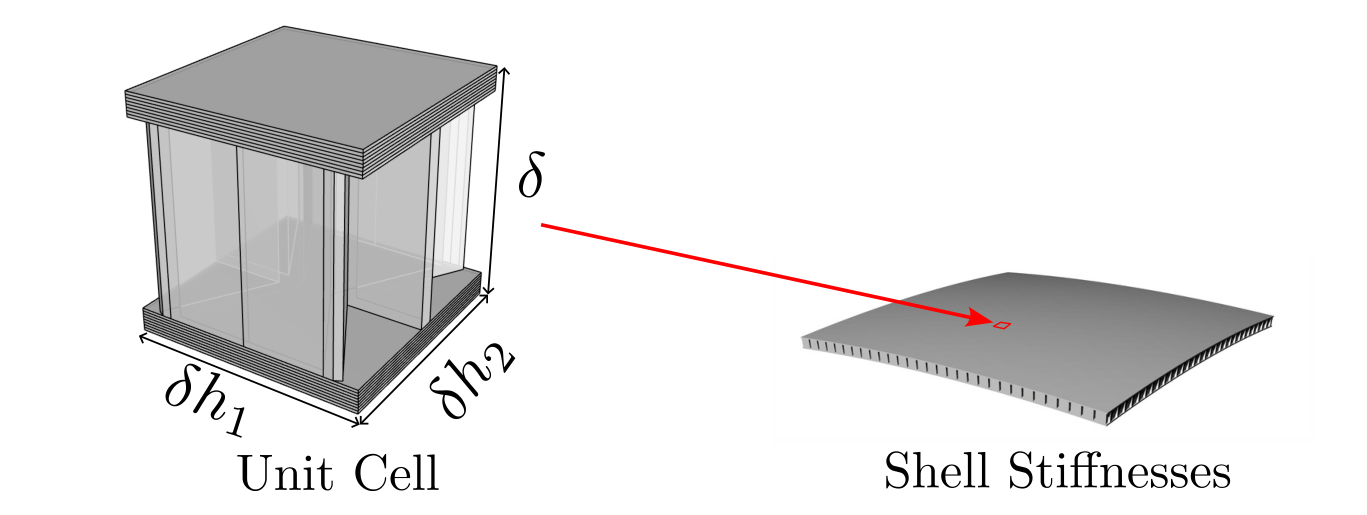
Figure 6.
Symmetry of the unit cell about the coordinate axes with a one-to-one mirroring of the boundary nodes on opposite faces.
Figure 6.
Symmetry of the unit cell about the coordinate axes with a one-to-one mirroring of the boundary nodes on opposite faces.
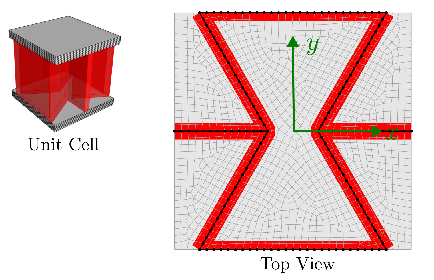
Figure 7.
ABD matrix of the sandwich section obtained with the two homogenization approaches: first-order homogenization combined with CLT (CLT-RVE, left) and NIAH (right).
Figure 7.
ABD matrix of the sandwich section obtained with the two homogenization approaches: first-order homogenization combined with CLT (CLT-RVE, left) and NIAH (right).
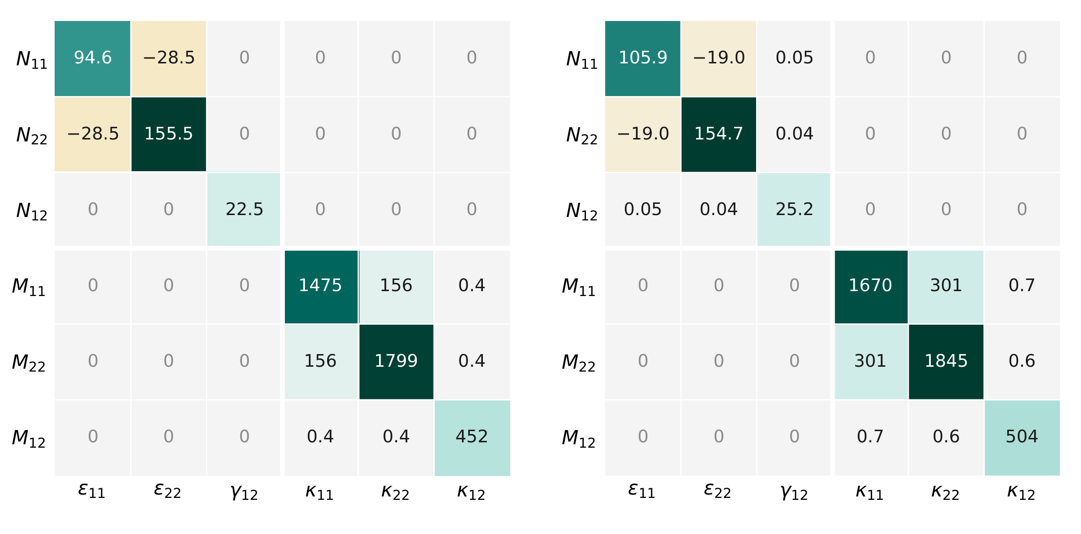
Figure 8.
Contribution of the auxetic core to the ABD matrix: first-order homogenization combined with CLT (CLT-RVE, left) and NIAH (right).
Figure 8.
Contribution of the auxetic core to the ABD matrix: first-order homogenization combined with CLT (CLT-RVE, left) and NIAH (right).
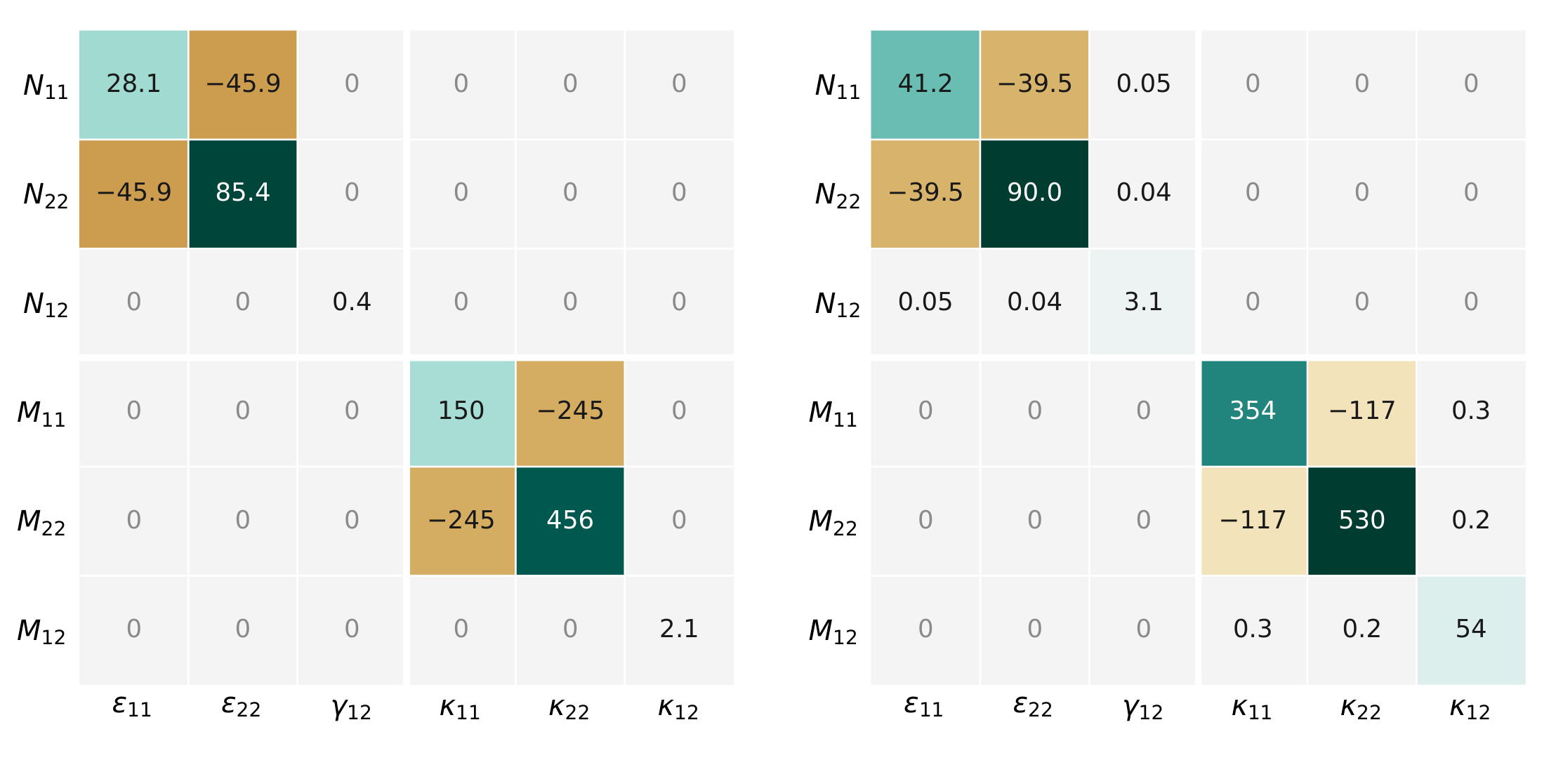
Figure 9.
Comparison of the displacement field for the resolved (a), first-order computational homogenization (b) and asymptotic homogenization (c) plate model under axial tension.
Figure 9.
Comparison of the displacement field for the resolved (a), first-order computational homogenization (b) and asymptotic homogenization (c) plate model under axial tension.
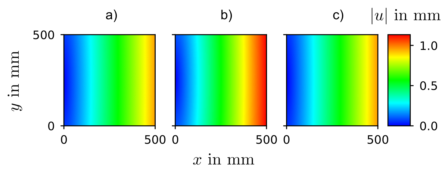
Figure 10.
Comparison of the displacement field for the resolved (a), first-order computational homogenization (b) and asymptotic homogenization (c) plate model under shear.
Figure 10.
Comparison of the displacement field for the resolved (a), first-order computational homogenization (b) and asymptotic homogenization (c) plate model under shear.
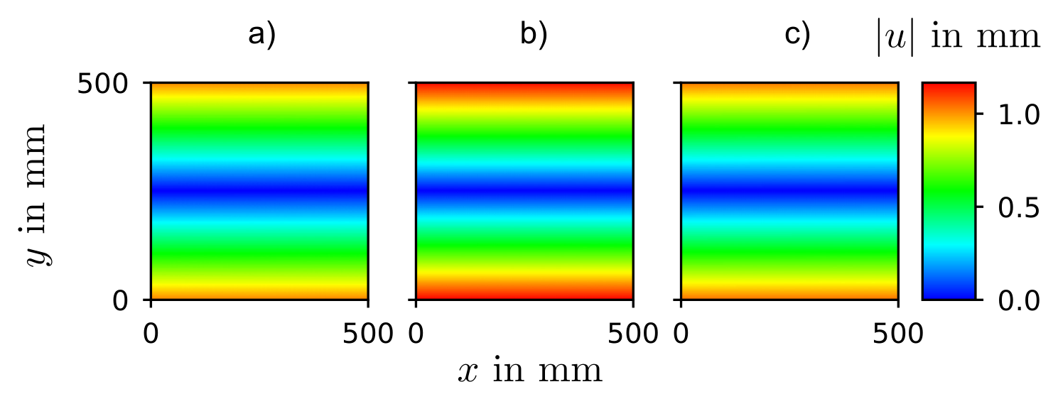
Figure 11.
Comparison of the displacement field for the resolved (a), first-order computational homogenization (b) and asymptotic homogenization (c) plate model under bending.
Figure 11.
Comparison of the displacement field for the resolved (a), first-order computational homogenization (b) and asymptotic homogenization (c) plate model under bending.
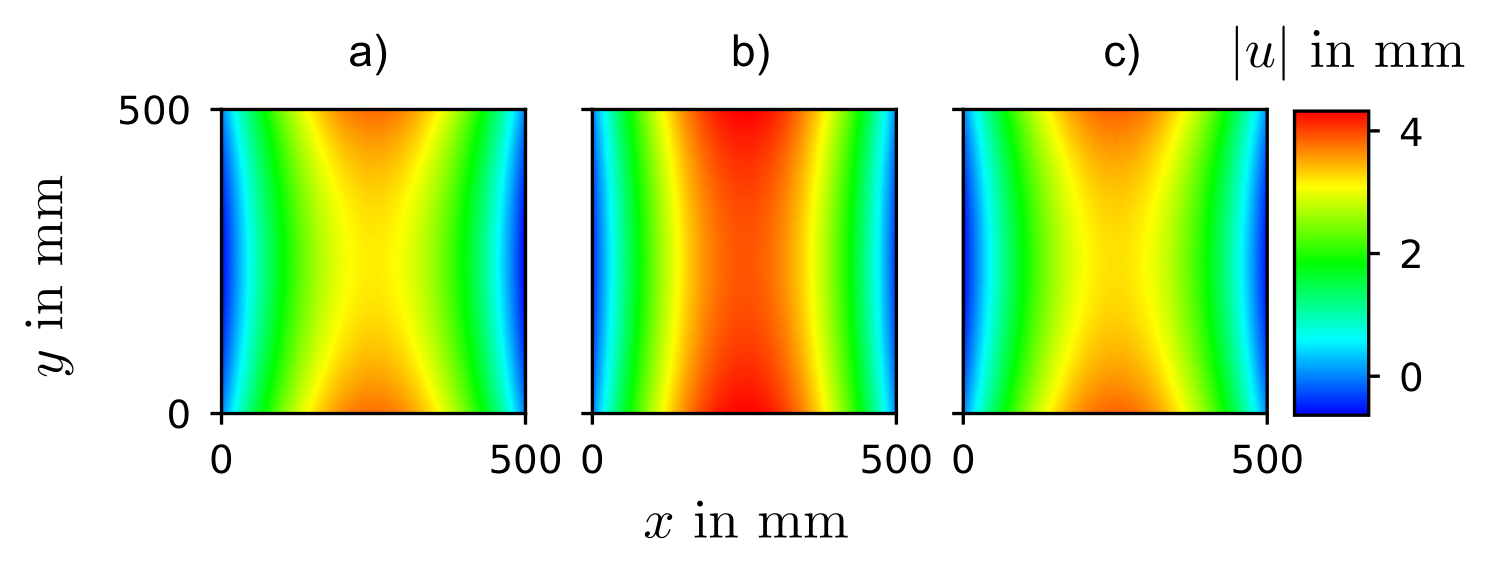
Figure 12.
Comparison of the mode shapes for the resolved (a), first-order computational homogenization (b) and asymptotic homogenization (c) plate model.
Figure 12.
Comparison of the mode shapes for the resolved (a), first-order computational homogenization (b) and asymptotic homogenization (c) plate model.
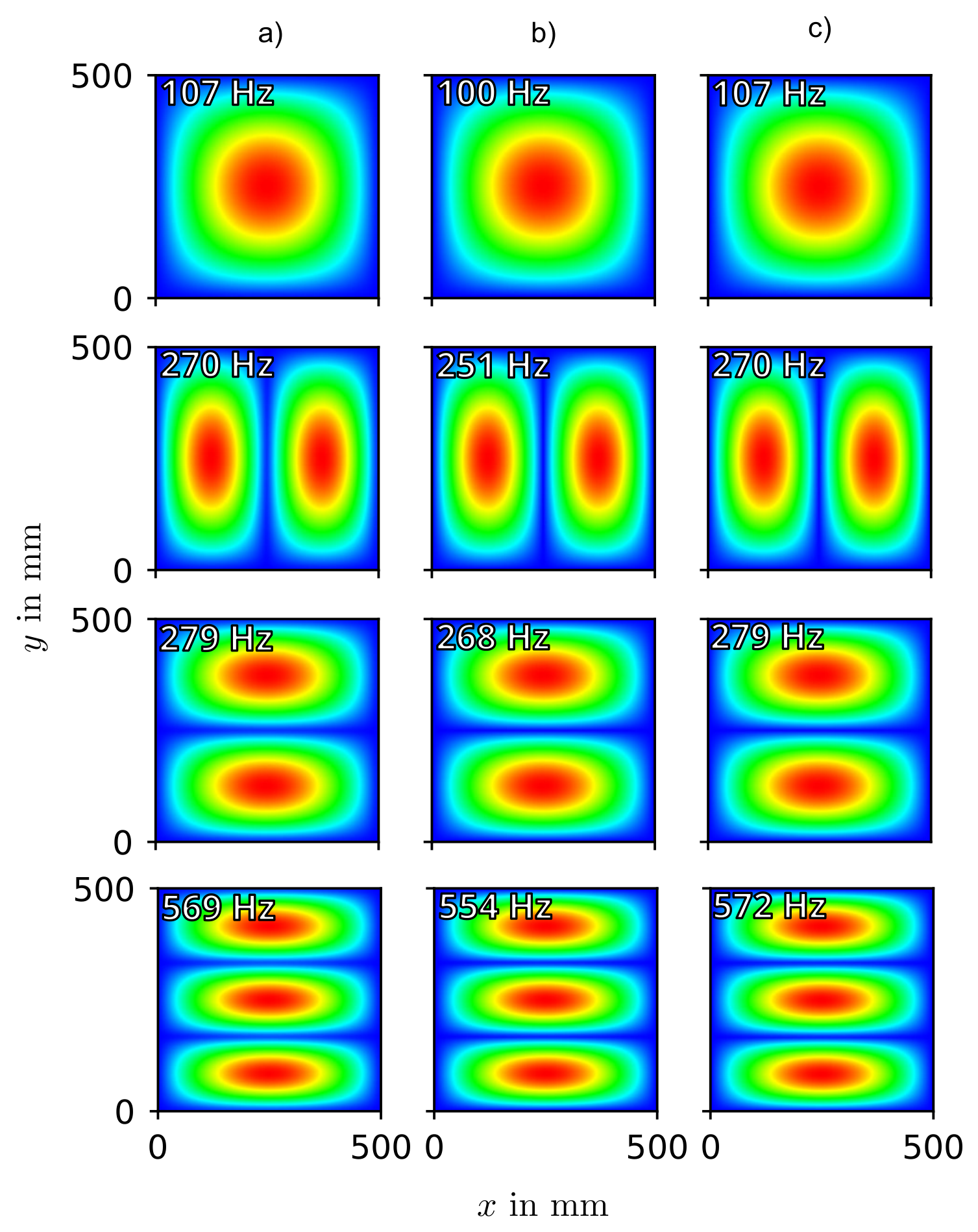
Figure 13.
Patch where the homogenized auxetic sandwich material properties are assigned.
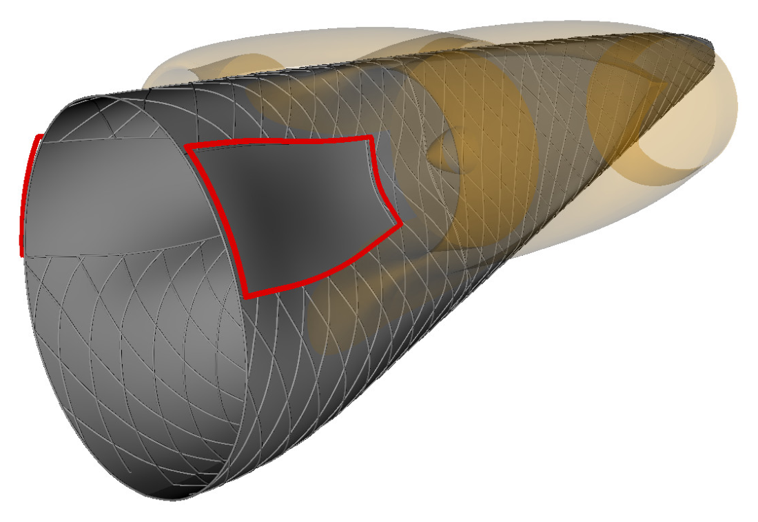
Figure 14.
Influence of the core topology and orientation on the deformation of the rear fuselage. (a) shows the displacement magnitude of the reference configuration, (b) to (d) the relative deviation of the displacement magnitude in percent with respect to (a).
Figure 14.
Influence of the core topology and orientation on the deformation of the rear fuselage. (a) shows the displacement magnitude of the reference configuration, (b) to (d) the relative deviation of the displacement magnitude in percent with respect to (a).
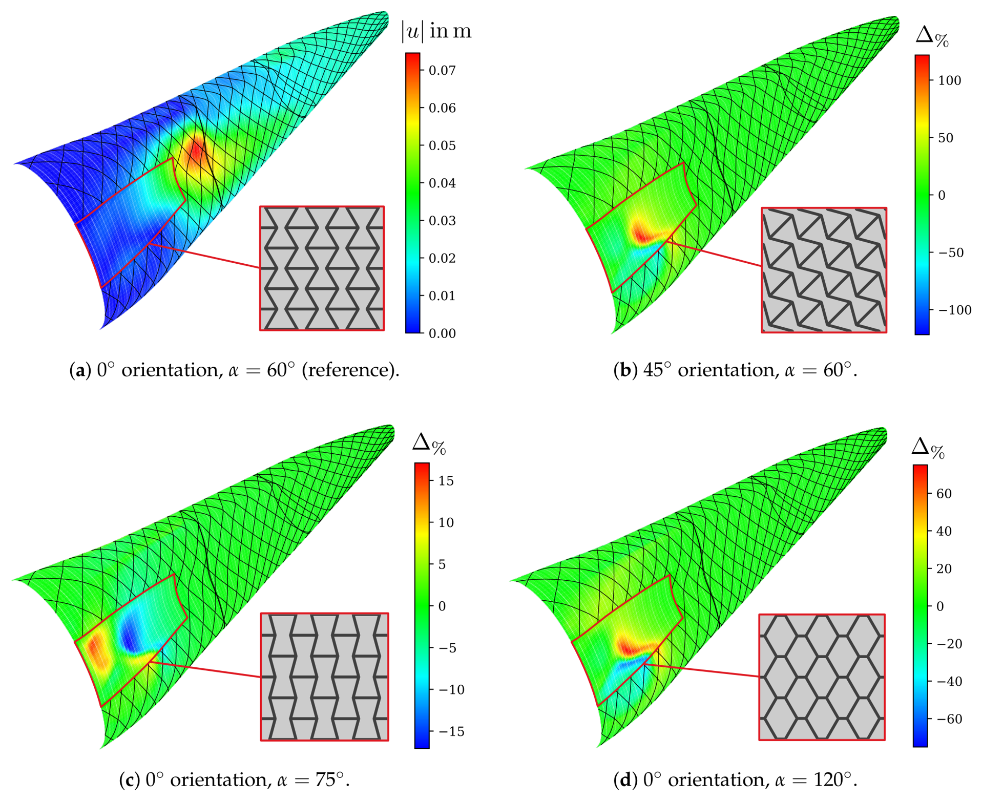

Table 1.
Geometric parameters of the re-entrant auxetic unit cell (see Figure 2).
Table 1.
Geometric parameters of the re-entrant auxetic unit cell (see Figure 2).
| w | h | H | t | |
|---|---|---|---|---|
| in mm | in mm | in mm | in degrees | in mm |
| 10 | 10 | 8 | 60 | 0.7 |
Table 2.
Boundary conditions in the RVE model for the six individual load cases. The in-plane cell dimensions w and h are listed in Table 1; is the RVE height.
Table 2.
Boundary conditions in the RVE model for the six individual load cases. The in-plane cell dimensions w and h are listed in Table 1; is the RVE height.
| DOF | Tension | Shear | ||||
|---|---|---|---|---|---|---|
| Interior Node (Suppressing Rigid-Body Motion) | ||||||
| 0 | 0 | 0 | 0 | 0 | 0 | |
| 0 | 0 | 0 | 0 | 0 | 0 | |
| 0 | 0 | 0 | 0 | 0 | 0 | |
| w | free | free | 0 | 0 | 0 | |
| 0 | 0 | 0 | 0 | 0 | ||
| 0 | 0 | 0 | 0 | 0 | ||
| 0 | 0 | 0 | 0 | 0 | ||
| free | h | free | 0 | 0 | 0 | |
| 0 | 0 | 0 | 0 | 0 | ||
| 0 | 0 | 0 | 0 | 0 | ||
| 0 | 0 | 0 | 0 | 0 | ||
| free | free | 0 | 0 | 0 | ||
Table 3.
Axial tension, N/mm. Strains according to Equation (13) in ; is the deviation from the resolved model.
Table 3.
Axial tension, N/mm. Strains according to Equation (13) in ; is the deviation from the resolved model.
| Resolved | CLT-RVE | % | NIAH | % | |
|---|---|---|---|---|---|
| DOFs | 7,083,614 | 75 | – | 75 | – |
| 1.9191 | 2.2368 | +16.6 | 1.9313 | +0.6 | |
| 0.2250 | 0.4100 | +82.2 | 0.2376 | +5.6 | |
| −0.1173 | −0.1833 | +56.3 | −0.1230 | +4.9 |
Table 4.
In-plane shear, N/mm. Shear strain according to Equation (14) in , effective stiffness in N/mm; is the deviation from the resolved model.
Table 4.
In-plane shear, N/mm. Shear strain according to Equation (14) in , effective stiffness in N/mm; is the deviation from the resolved model.
| Resolved | CLT-RVE | % | NIAH | % | |
|---|---|---|---|---|---|
| DOFs | 7,083,614 | 75 | – | 75 | – |
| 4.0383 | 4.6646 | +15.5 | 4.1589 | +3.0 | |
| 26,001 | 22,510 | −13.4 | 25,247 | −2.9 |
Table 5.
Pure bending, N mm. Curvatures in /mm; is the deviation from the resolved model.
| Resolved | CLT-RVE | % | NIAH | % | |
|---|---|---|---|---|---|
| DOFs | 7,083,614 | 75 | – | 75 | – |
| 1.2148 | 1.3809 | +13.7 | 1.2339 | +1.6 | |
| −0.2041 | −0.1345 | −34.1 | −0.2011 | −1.5 | |
| 0.1681 | 0.0974 | −42.0 | 0.1630 | −3.0 |
Table 6.
Modal analysis, simply supported edges. Frequencies of the first three bending modes in Hz; all mode pairs have . Mode numbers refer to the resolved model, whose in-plane mode 2 is omitted; is the deviation from the resolved model.
Table 6.
Modal analysis, simply supported edges. Frequencies of the first three bending modes in Hz; all mode pairs have . Mode numbers refer to the resolved model, whose in-plane mode 2 is omitted; is the deviation from the resolved model.
| Resolved | CLT-RVE | % | NIAH | % | |
|---|---|---|---|---|---|
| DOFs | 7,083,614 | 1200 | – | 1200 | – |
| Mode | 107.0 | 100.4 | −6.2 | 107.1 | +0.0 |
| Mode | 269.6 | 251.7 | −6.6 | 270.2 | +0.2 |
| Mode | 278.6 | 269.2 | −3.4 | 279.1 | +0.2 |
| Mode | 569.1 | 557.6 | −2.0 | 571.5 | +0.4 |
Disclaimer/Publisher’s Note: The statements, opinions and data contained in all publications are solely those of the individual author(s) and contributor(s) and not of MDPI and/or the editor(s). MDPI and/or the editor(s) disclaim responsibility for any injury to people or property resulting from any ideas, methods, instructions or products referred to in the content. |
© 2026 by the authors. Licensee MDPI, Basel, Switzerland. This article is an open access article distributed under the terms and conditions of the Creative Commons Attribution (CC BY) license (http://creativecommons.org/licenses/by/4.0/).
Copyright: This open access article is published under a Creative Commons CC BY 4.0 license, which permit the free download, distribution, and reuse, provided that the author and preprint are cited in any reuse.