

Submitted:
15 October 2026
Posted:
16 October 2026
You are already at the latest version
Abstract
Geological CO₂ storage requires compressibility assumptions suited to the effective-stress interval and loading path. We assess their adequacy by separating curve approximation, prediction, parameter identification, and storage consequence. An exact minimax bound tests when a constant logarithmic slope cannot meet a specified tolerance. Across 19 published sediment trajectories, full-data calibration of Arc Joint via Optimum Parameters (AJOP) gave a median range-normalized void-ratio RMSE of 1.27% and a maximum of 3.41% for its five-parameter form; 12 fits selected its exact linear member. The quadratic had a lower median error but locally reversed compression in four cases. Separate blocked tests, thirteen independent Boston Blue Clay specimens, and an intact Draupne record expose limits on prediction and transfer. In twelve archived Smeaheia scenarios, compressibility choices changed pressure-screen classifications. The assessment connects tests of simple assumptions, the value of added curvature, and calibration requirements to storage screening, while preserving the distinction between successful loading-curve approximation and field validation.
Keywords:
geological CO₂ storage
; compressibility
; effective-stress interval
; AJOP
; linear approximation
; calibra-tion
; pressure screening
1. Introduction
Geological CO₂ storage assessments must establish whether pressure buildup remains compatible with containment and the intended injection operation [1,2,3,4,5,6]. Compressibility assumptions enter this assessment through pore-volume change and skeleton deformation. Their adequacy must be judged against the accuracy required of the engineering output.
Effective stress connects these processes [7,8,9,10]. At approximately fixed total stress, rising pore pressure unloads the skeleton. Lateral constraint, pressure gradients, and thermal contraction produce different paths elsewhere in the reservoir–caprock system [10,11,12,13,14,15,16]. In Frio sand, Zheng and Espinoza [17] measured distinct pore-volume compressibilities for loading and unloading under different confinement conditions; using an inappropriate value underestimated injection-induced pressure buildup in their reservoir simulations. The calibration path is therefore part of the property specification.
Field observations at In Salah, Sleipner, and Weyburn demonstrate that geometry, pressure communication, and rock properties influence deformation [15,18,19,20]. Assessments of induced seismicity also depend on the initial stress state and pressure change [21,22,23]. Pressure management can form part of the integrity strategy [24].
A common practical choice is to assign one compressibility when laboratory information is sparse. In the Smeaheia archive, three constant pore-volume compressibilities spanning two orders of magnitude produced markedly different pressures [25,26,27]. Using the same site dataset, Wang et al. [28] quantified uncertainty in storage efficiency under volume and pressure constraints. Thermal effects, uncertain properties, loading rate, coupling, and nonlinear elasticity add further uncertainty [16,29,30,31,32]. Such assessments motivate examining the evidence behind an assigned property as well as propagating its assumed range.
A logarithmic void-ratio slope, a constrained compressibility, a pore-volume compressibility, and a constrained modulus are related but are not interchangeable. A straight line in void ratio versus log stress does not imply constant stiffness. Lee et al. [33] linked measured pore and bulk compressibilities to analytical estimates of storage efficiency and deformation, illustrating the importance of property definitions and mechanical constraints. Rate effects, nonlinear shale response, and pore-structure changes introduce further distinctions [30,32,34,35,36]. An accurate curve can also have an inaccurate derivative, so representation and tangent-property adequacy require separate checks.
Clay-rich sediments exhibit responses ranging from nearly linear to strongly curved over laboratory stress windows. Fabric, bonding, stress history, mineralogy, and porosity influence that response [37,38,39,40,41,42,43]. Resedimented mudrocks help isolate composition from natural structure [44,45,46,47,48]. Casey et al. found that preferred compression relations differed among 15 resedimented materials [45]. This motivates comparison across curve shapes while preserving the distinction between many locations on one trajectory and independent specimens.
The square-root transition introduced by Kaewhanam and Chaimoon [49] was developed as Arc Joint via Optimum Parameters (AJOP) for clay consolidation by Phonchamni et al. [50] and used in AJOP-T hardening by Chatwong et al. [51]. The family provides a common setting for evaluating linear and nonlinear compression: it represents a curve approaching a straight branch and includes an exact straight-line member. We evaluate the four-parameter form and a centered five-parameter extension with independent limiting slopes. The curved-function comparator in Phonchamni et al. is a positive-exponent power relation, distinct from the quadratic in log stress tested here.
This structural breadth does not imply that one AJOP parameterization can reproduce every curvature exactly. The present nonnegative slope-contrast form has a nonincreasing void-ratio derivative in log stress. A slightly concave-up response may therefore be approximated by its linear member, with the remaining error reported explicitly. Material state and branch remain separate limits: an intact bonded sediment, a resedimented mixture, and an unloading path need not share one envelope [37,38,39,52,53].
Three open sources provide 19 loading trajectories for a direct test of representation: six resedimented Nankai mixtures [54], five incremental-loading records from Sites C0011 and C0012 [55], and eight sediment–diatom mixtures [56,57]. We supplement these curve-level comparisons with independent Boston Blue Clay specimen endpoints [58], an intact Draupne oedometer record [59,60], and archived Smeaheia pressure scenarios [26,27]. The external trajectories broaden the shape test; they are not Smeaheia material calibrations.
The methodological question is how to test the evidence supporting a compression approximation before using its derived properties in a storage assessment. Complete-window residuals describe representation; stress-blocked tests address prediction; parameter diagnostics address identification [61,62]. Material changes, including geochemical alteration, further limit transfer [63]. These distinctions complement storage-scale uncertainty analysis: a plausible range of property values does not establish that the chosen constitutive form or calibration window supports the intended use.
We address this question through an exact minimax bound for constant logarithmic slope, full-window comparisons across 19 linear and curved loading trajectories, and separate prediction and identification tests under restricted calibration. AJOP supplies a common family that includes a reduced linear member and a curved-to-linear transition. Draupne branch measurements and archived Smeaheia pressures then illustrate property-path and screening consequences. The contribution is a reproducible assessment of approximation and calibration evidence; these complementary tests do not form a single laboratory-to-reservoir validation chain. Figure 1 places the assessment within the storage problem.
2. Stress-Dependent Compression Framework
2.1. Effective Stress and the Meaning of “Compressibility”
For one-dimensional constrained compression, effective vertical stress is written as
where is total vertical stress, is pore pressure, and is Biot’s coefficient [7,8,9]. Compression is taken as positive. The distinction among commonly conflated properties is
and
Here, is the local logarithmic compression slope, is constrained compressibility, is pore-volume compressibility, is compressive logarithmic volumetric strain, and is pore volume. The derivative in Equation (3) is defined with respect to effective vertical stress along the constrained laboratory path. A reservoir ROCK input refers to pore-volume response under the simulator’s pressure and stress assumptions; it is not obtained from Equation (3) without specifying those assumptions. Let denote the constant solid volume. Assuming incompressible solids and one-dimensional strain, and . The exact logarithmic strain relative to a reference state is
These definitions prevent a constant , a constant , and a constant from being treated as equivalent null models. Here is the void ratio at the strain-reference state; it is distinct from the transition-state parameter introduced below. A logarithmic stress derivative means differentiation with respect to the logarithm of stress divided by a fixed positive reference stress.
2.2. A Centered Two-Asymptote Extension of AJOP
Starting from the AJOP family [49,50,51], let
where is the transition stress. Define and the centered transition function
The centered AJOP-family loading envelope is
The centering term is essential: it makes . Without it, cannot be interpreted as the void ratio at the transition stress. The remaining parameters are the low-stress slope , high-stress slope , and positive dimensionless transition-width parameter . For monotonically increasing compression slope, the admissible ordering is . With a zero low-stress slope, Equation (7) recovers the earlier four-parameter shape after centering and parameter rescaling.
The physically admissible loading domain is restricted to positive effective stress and positive void ratio. The asymptotic slopes are mathematical limits of the model; they do not imply physical validity at arbitrarily large stress.
Differentiation gives the local slope
and its evolution with log stress,
For , is exactly the stress at which the slope is halfway between its asymptotes, and the maximum rate of slope change is at . The stresses at which 10% and 90% of the slope transition have occurred define an exact transition band,
The minus sign gives and the plus sign gives . This band locates the central part of the loading-slope transition. Intersecting does not alone prove failure of a constant; the slope contrast over the actual interval must be tested. When , the slope is constant and no distinct 10–90% transition band can be identified; Equation (10) is then not a transition diagnostic.
For incompressible solids, the derivative-consistent quantities passed to a constrained geomechanical calculation are
The tangent constrained modulus is
Equations (11) and (12) show why even an asymptotically constant does not imply constant , , or . Equation (12) requires . If the slope vanishes, constrained compressibility is zero and the modulus is understood as an infinite-stiffness limit.
2.3. An Exact Failure Bound for a Constant Slope
Suppose the stress domain is broad enough to sample both asymptotic slopes and . Minimizing the maximum absolute relative slope error over the two limiting values gives
Here, is the minimax constant and is its unavoidable worst-case relative error at the two asymptotes. For an allowable relative slope error with , no constant slope can satisfy the tolerance across both regimes if
At , failure is guaranteed when . If , a relative bound is undefined and the minimum maximum absolute slope error is . Equations (13) and (14) are constitutive bounds; storage-scale failure still requires propagation to an engineering output.
For the positive-slope case, restrict the candidate constant to the interval between the two slopes: a value outside it cannot reduce the maximum error. At the minimizer, its relative overprediction at the lower slope equals its relative underprediction at the higher slope. Solving this equality gives the harmonic mean in Equation (13). For any intermediate slope, the absolute relative error is no greater than the larger endpoint error, which proves the minimax result. On a finite stress interval, the same argument applies exactly to the minimum and maximum local slopes on that interval; the asymptotic values should be used only when they are justified.
2.4. Null Models and Equal-Footing Competitors
The reference comparisons use a constant logarithmic slope, a constant constrained compressibility, the nested AJOP form, and an empirical mudrock relation. The expanded trajectory analysis also includes a quadratic in log stress, a constrained monotone quadratic, and the positive-exponent curved function used by Phonchamni et al. [50]. The baseline relations are:
1. a constant log-slope relation, ;
2. a constant constrained-compressibility law, ; here the starred stress and void ratio specify the same reference state, and the constant constrained compressibility is positive.
3. the nested AJOP form obtained from Equation (7) by setting ;
4. the published five-parameter empirical mudrock model of Uyeturk and Germaine [47].
Every comparison minimizes the same unweighted sum of squared void-ratio residuals and uses the same locations within that comparison. Full-data error measures representation over the fitted interval. Held-out error measures prediction under the specified partition. Information criteria and sensitivity diagnostics address different questions [61,62]; a lower calibration error does not establish parameter identification. For the interpolated trajectory locations, we report descriptive errors without treating those locations as independent specimens.
2.5. Linear Members and Calibration-Window Interpretation
The centered AJOP5 family includes a globally linear member when . Equation (7) then becomes
The four-parameter member has . Its zero-curvature limit gives a horizontal branch below the reference stress and a straight descending branch above it. Over a window entirely on the descending branch,
This is the linear limit discussed by Phonchamni et al. [50], expressed in the present centered coordinates. Setting the curvature parameter to zero therefore produces a sharp corner if the transition lies inside the window; it does not remove that corner globally. To fit a wholly linear window, we fix the reference stress at the lowest observed stress. The fitted line then has two effective parameters, and its unobserved transition location is not estimated.
The fitting strategy should follow the information in the window. A curved early segment may constrain curvature while leaving the eventual linear slope uncertain. Additional observations must extend far enough to resolve that slope, rather than merely add points within the same early segment. Conversely, a nearly straight window can support a line without supporting a transition location. It may represent a low-stress branch, a high-stress branch, or a narrow part of a smooth curve.
3. Materials and Methods
3.1. Published Trajectories and Full-Window Calibration
The external benchmark contains 19 trajectories grouped by source. P01–P06 are six resedimented Nankai mixtures from Reece et al. [54]. P07–P11 are five incremental-loading records from Hüpers and Kopf [55], comprising four natural silty-clay samples and one remolded sample (P08). P12–P19 are eight resedimented BBC and Eugene Island (EI) mixtures from Scott and Reece [56,57], including lacustrine or marine diatomaceous earth (LDE or MDE). The source register gives specimen identifiers, workbook sheets, columns, units, extraction rules, and file hashes. These materials broaden the curve-shape comparison without being treated as site-specific storage rocks.
For the fourteen continuous trajectories, void ratio was interpolated linearly in log stress at the frozen evaluation locations. The six Nankai windows span 0.2–20 MPa and the eight Scott–Reece windows span 0.2–1.8 MPa, with 40 derived locations per curve. The five incremental-loading curves retain 9 or 10 source endpoints spanning 0.12–16 or 20 MPa. All locations in these windows enter the full-data fit. The continuous measurements are also shown as pale background traces in the figures. Derived locations are numerical evaluation points, not additional experiments or independent replicates.
Six forms were calibrated for every complete trajectory: log-linear, quadratic in log stress, a quadratic constrained to remain monotone and positive over the fitted interval, positive-exponent CF power, AJOP4, and AJOP5. The CF form follows the power-law comparator of Phonchamni et al. [50]; its nonnegative exponent ranges from zero, the logarithmic limit, to five. The quadratic constraint is imposed at both interval endpoints on its derivative and at the upper endpoint on void ratio. Because a quadratic derivative is linear, the endpoint inequalities enforce monotonicity throughout that interval.
AJOP estimation profiles out the linear coefficients by bounded conditional least squares and searches the two shape coordinates. The reference stress remains within the observed calibration window; the smooth curvature parameter ranges from 0.0001 to 100. Linear coefficients lie between zero and the larger of 2 and twice the maximum observed void ratio. An 81 by 81 shape grid, 24 local starts, and four differential-evolution seeds provide independent numerical checks. The exact linear candidates in Equations (15) and (16) are included explicitly. A linear boundary is selected only when its squared-error objective is no greater than the smooth optimum to numerical precision. No general zero-curvature kink is fitted in this benchmark.
The previous primary stress blocks are preserved separately. For continuous curves, 25 lower-stress locations formed calibration and 15 higher-stress locations formed prediction; cutoffs were approximately 5 MPa for P01–P06 and 0.8 MPa for P12–P19. For P07–P11, the first seven endpoints through 8 MPa formed calibration, leaving two or three higher-stress endpoints. Bounds and fitting inputs were obtained from those training windows. These blocked comparisons, alternative cutoffs, and interior holdouts are retained unchanged in S1 and S2. The full-window extension is exploratory and uses responses that were withheld in those earlier tests; it is not a new prospective validation.
3.2. Draupne, RBBC, and Smeaheia Data Provenance
The laboratory evidence is the open replication dataset for the Draupne shale test program [59,60]. The oedometer specimen was cut normal to bedding, had an initial height of 20.34 mm and diameter of 50.35 mm, and had a reported initial porosity of 18.92%. The repository file contains 22,724 chronological observations of elapsed time, vertical strain, pore pressure, and effective vertical stress. The SHA-256 hashes, original filenames, and processing environment are recorded in Supplementary File S1.
The independent-specimen evidence was transcribed from Table 5-1 (p. 153) of Casey’s open doctoral thesis [58]. Each row identifies a separate resedimented Boston Blue Clay triaxial specimen and reports its terminal pre-shear state; ideal -consolidation is not assumed for every specimen. The primary cohort retained specimens with finite effective vertical stress and void ratio and excluded the three tests flagged in the source as having high excess pore pressure during consolidation. Thirteen specimens remained, spanning 0.198–101.25 MPa. These values are terminal states from separate preparations, not repeated observations along one continuous curve. The complete 27-row transcription, source-row notes, and inclusion flags are preserved in Supplementary File S1.
Stable endpoints were defined as the median of the final 60 min of each documented hold. The six successive primary-loading maxima were 10.98, 15.00, 22.49, 33.76, 50.63, and 75.96 MPa. The chronology also contained unloading from 33.76 to 22.49 MPa, reloading to 33.76 MPa, and final unloading through 50.62, 33.75, and 22.48 MPa. The calculation was repeated with 30 and 120 min endpoint windows to test processing sensitivity. These windows measure endpoint repeatability; they do not represent specimen-to-specimen uncertainty.
The reported strain is engineering vertical strain in millistrain. With one-dimensional deformation and incompressible solids, a reference-shifted void ratio was reconstructed from . The reported 18.92% porosity gives , which was assigned to the first stable endpoint because the strain channel is effectively zero there. Here is engineering strain relative to that first endpoint. For the reconstruction, in Equation (4), so . This convention fixes both the void-ratio offset and the conversion factor from engineering strain to void ratio. The measured engineering-strain increments are unchanged by that choice, whereas absolute void-ratio increments and errors scale with one plus the assigned reference void ratio. For this reconstruction, the logarithmic strain depends only on the measured engineering strain.
The storage evidence is the official Smeaheia reference archive [26] and the associated field-scale study [25]. The pressure benchmark is Table 5-2 of the Troll Kystnær Subsurface Status Report, revision 03 (2012) [27]. It reports pressure buildup after 50 years of 3.2 Mt injection for three pore-volume compressibilities and four connected-volume cases. The twelve values and the compressibility inputs in Section 5.1 of the source report [27] were checked directly against that report and transcribed into the machine-readable table. No new reservoir simulation is performed here.
3.3. Numerical Estimation and Parameter Diagnostics
The Draupne analysis evaluated six models in void-ratio space: constant logarithmic slope; constant constrained compressibility; a quadratic in log stress; the nested form of Equation (7) with ; the unrestricted five-parameter transition law; and the five-parameter Uyeturk–Germaine relation [47]. The RBBC specimen-level screen evaluated the same two constant models, the quadratic, and both five-parameter laws. All models used unweighted void-ratio residuals. The exponential constant constrained-compressibility relation follows from Equations (2) and (4). Linear regression of against effective stress supplied only its initial guess; the final parameters minimized unweighted squared residuals in , using an analytical Jacobian. Thus the response transformation did not change the fitting objective relative to the competitors.
For the Draupne and RBBC analyses, nonlinear models were estimated by bounded least squares with deterministic multistart initialization. For the transition law, , and were non-negative, was restricted to the fitted stress interval, and . Ninety starting points were used for the principal Draupne fits. For RBBC, full-data fits used 32 starts, blocked-training fits used 40, and leave-one-specimen-out refits used 32 starts constructed solely from each training fold. No fit to the complete dataset supplied a cross-validation starting point. Stress-dependent bounds in blocked and leave-one-out fits were also obtained only from the training observations. For the Uyeturk–Germaine comparator, the offset is subtracted and may be signed; positivity of the infinite-stress void ratio is not imposed. Its finite fitting bounds are study-specific. Supplementary File S1 documents the source-equation convention, parameter mapping, seeds, bounds, and transformed parameterizations.
Model diagnostics were root-mean-square error (RMSE) and mean absolute error in void ratio, leave-one-out cross-validation for the three low-order models, the corrected Akaike information criterion () [61], and the Bayesian information criterion [64]. For , the fitted residual variance was counted as a parameter. was reported as undefined when , where includes that variance term. This rule prevents a nearly saturated five-parameter fit to six endpoints from being presented as information-criterion evidence. and BIC use the Gaussian residual score with the common additive constant omitted. These are descriptive comparisons under a working independent, equal-variance error model, not tests of physical identification. The nominal five-parameter score is not interpreted for the RBBC transition fit because collapse to a constant slope makes its parameterization singular.
Practical identifiability was evaluated from the column-scaled local sensitivity matrix and by profile likelihood [62]. The transition stress was fixed at 64 logarithmically spaced values from 10.98 to 75.96 MPa while the remaining parameters were reoptimized. A nominal 95% likelihood-ratio threshold was plotted for diagnosis. Because the unrestricted fit has only one residual degree of freedom, this threshold is not treated as a population confidence interval. Nominal 95% -based intervals were calculated for the two-parameter constant models; the constant-compressibility interval used a local Jacobian linearization of its nonlinear least-squares fit. These intervals are conditional on the working residual model and do not quantify between-specimen uncertainty.
3.4. Draupne High-Stress Holdout and Endpoint-Window Sensitivity
The tail holdout used a fixed stress-based partition. The first five primary-loading endpoints, from 10.98 to 50.63 MPa, were used for calibration, and the 75.96 MPa endpoint was predicted without refitting. Absolute error in void ratio was reported together with the error as a percentage of the observed void-ratio change from 50.63 to 75.96 MPa. A model with parameters was not assigned a holdout result when the number of calibration observations was no greater than . Under this rule, neither five-parameter law can be validated by a five-point calibration even if an optimizer returns a number.
The complete calculation was repeated with 30, 60, and 120 min endpoint windows. A result was regarded as processing-stable when its interpretation did not change across these windows. Local slopes were calculated only between stable raw-data endpoints; no numerical derivative of a digitized curve was used. For adjacent endpoints, interval properties are and , with any fixed positive in the logarithmic difference. They are secants, not pointwise tangents.
3.5. Independent-Specimen RBBC Stress Test
The specimen-level high-stress block used a fixed 10 MPa threshold. Ten specimens consolidated at formed the calibration cohort, and three specimens above 10 MPa formed the test cohort. Because the 10 training specimens exceed , both five-parameter laws could be evaluated out of sample. This count permits a numerical prediction; it does not by itself establish parameter identification. Full-data RMSE, , BIC, leave-one-specimen-out (LOSO) RMSE, and blocked high-stress RMSE were reported separately.
Cohort sensitivity was evaluated with two explicit alternatives. A strict- cohort also required and retained 11 specimens. An inclusive cohort reinstated the three source-flagged high-excess-pore-pressure tests and retained 16 specimens. An additional source-audit sensitivity excluded TX1030 because Casey identifies its stress-ratio response as erroneous (p. 149); this left 12 specimens, with nine for training and three for the blocked test. The primary cohort was retained because the source warning does not specifically invalidate its endpoint stress or void ratio. No derivative was estimated from these discontinuous specimen endpoints. The test therefore evaluates prediction of terminal void ratio within one resedimented material, not a continuous constitutive trajectory or transfer across mudrocks.
3.6. Loading, Unloading, and Reloading
Equation (7) is a primary-loading envelope. It was not used to represent injection-induced unloading. Secant moduli were calculated separately for the observed first unloading, reloading, high-stress unloading, and later unloading stages. This separation is required because, at approximately fixed total vertical stress, a pore-pressure increase reduces effective stress. Pressure dissipation may later reload the same material [10,16,37,38,39].
For the reduced-order storage screen, the published Draupne unloading values of 3.8 and 8.3 GPa were retained as branch bounds [59]. They are not combined with the primary-loading fit, and they are not treated as Smeaheia-specific measurements.
3.7. Smeaheia Archival Benchmark and Reduced-Order Screen
The official report evaluated pore-volume compressibilities of , , and because no Smeaheia laboratory constraint was available [26,27]. Connected water volumes were 51, 160, 297, and 418 . The present analysis preserves the twelve reported pressure outcomes and compares all twelve cases with the updated report screens, evaluated at 900 m TVDmsl, of 33 bar for a caprock containing pre-existing fractures and 65 bar for intact Draupne shale.
The original pressure table was colour-coded against an earlier 20 bar criterion. The present classifications are recalculated from the archived pressures using the later assessment in Section 4.7 of the same report: 33 bar in its narrative summary (33.1 bar in Table 4-2) for the base minimum-stress case, and 65 bar for the low-case intact-rock fracture-initiation model. Neither screen includes thermal stress effects [27].
A one-dimensional end-member was added to show the deformation scale without claiming a coupled field solution. At 1260.5 m TVD/KB (1236.5 m TVDmsl, with a 24 m Kelly Bushing elevation), the archived March 2017 stress model gives overburden and pore-pressure equivalent mud weights of 1.826 and 1.011 specific gravity [26]. Using its native TVD/KB convention gives an initial effective vertical stress of 10.074 MPa when Biot’s coefficient is set to one. This is an explicit end-member assumption, not a measured site value of that coefficient. Using the 79 and 129 m well thicknesses reported for 32/2-1 and 32/4-1 as illustrative endpoints [27], together with unloading modulus , conditional rebound was calculated to first order as , at fixed total vertical stress and with Biot’s coefficient set to one. For another specified coefficient, the effective-stress decrement and this first-order rebound are multiplied by that coefficient. These thickness endpoints are not site-wide minimum and maximum bounds. The transmission factor lies between zero and one: denotes no caprock pore-pressure transmission, whereas applies the full reservoir pressure increment uniformly as an upper end-member. The constrained modulus represents zero lateral strain. The calculation does not resolve spatial pressure gradients, site-scale lateral coupling, thermal stress, faults, or poroelastic total-stress redistribution.
3.8. Evaluation Criteria
Table 1 separates approximation, prediction, identification, tangent properties, and engineering consequence. For the 19-trajectory full-data analysis, RMSE and maximum absolute error are normalized by the observed void-ratio range of each complete evaluation window. The 1%, 2%, and 5% RMSE levels are illustrative sensitivity bands, not independently justified acceptance limits. They were examined during this exploratory reanalysis. A project-specific tolerance must instead follow the error permitted in the intended engineering output.
A useful approximation can remain within a stated curve-error band without being the best-fitting model. Suitability also depends on maximum local error, derivative behavior, and the intended calculation. For a nearly straight observed window, a reduced AJOP member avoids estimating unnecessary transition parameters. If the window begins in a transition, calibration should sample enough of the subsequent branch to constrain its slope before high-stress prediction is interpreted. These are calibration principles to be tested, not a prospectively validated selection rule. A straight initial segment alone cannot locate it relative to an unobserved transition.
3.9. Reproducibility
Supplementary File S1 supplies the source records, fitting protocols, parameters, pointwise predictions, numerical tables, and figure scripts. File S2 groups full-data calibration, blocked prediction, cutoff and interior-holdout sensitivities, parameter searches, and exploratory refits. The v20 checks read the actual manuscript, compare reported metrics with CSV outputs, verify citation order and native mathematics, and confirm preservation of equations, tables, figures, and the original bibliography entries from v19. A checksum manifest identifies the files. Historical outputs retain their original protocols and are not pooled into a new prediction score.
4. Results and Discussion
4.1. Constant-Slope Approximation Bound
Equations (10)–(14) separate the location of a slope transition from a proof that a constant fails. The 10–90% band locates the central transition, but crossing that band is not a sufficient failure criterion. For any specified interval with positive slopes, Equation (13) applies with its actual minimum and maximum slopes. A constant is excluded at tolerance only when their ratio exceeds . The asymptotic form in Equation (14) is the limiting result when both asymptotes are represented. Figure 2 shows these dataset-independent relationships; loading-envelope bounds are not applied to an injection-unloading branch.
This result also explains why calibration-window choice matters. A constant fitted at low stress tends to overpredict stiffness after the slope has increased, whereas a high-stress constant tends to underpredict stiffness at low stress, when the comparisons are made at the same stress and void ratio. A secant fitted across the full window can reduce void-ratio residuals while retaining biased tangents at both ends. At a common stress and void ratio, the relative errors in constrained and pore-volume compressibility equal the relative error in the local logarithmic slope. If competing models predict different void ratios, the additional void-ratio denominators also affect the tangent-property errors.
4.2. Linear and Nonlinear Approximation Across Nineteen Trajectories
Table 2 and Figure 3, Figure 4, Figure 5, Figure 6, Figure 7 and Figure 8 address the representation level of the adequacy assessment, using every trajectory grouped by source. AJOP5 gave a median normalized RMSE of 1.27% and a maximum of 3.41%. Eight curves were within 1%, fourteen within 2%, and all nineteen within the illustrative 5% band. The largest pointwise discrepancy was 7.64% of the observed void-ratio range, showing why a small average error should not be used alone. AJOP4 had the same 14-of-19 and 19-of-19 counts at 2% and 5%, respectively, with a median of 1.43%.
The constrained fits selected the exact linear member for twelve AJOP5 cases and thirteen AJOP4 cases. This is a reduction within the family, not a failed optimization or proof that the true response has zero curvature. In the Reece group, five of six AJOP5 fits were linear; their normalized RMSE ranged from 1.43% to 3.41%. The quadratic followed the gentle concave-up shape more closely. The linear AJOP approximation remains quantifiable and may be adequate for a stated purpose, but the illustrative bands cannot determine that purpose-specific tolerance.
The natural incremental-loading curves contain clearer curvature and changes in slope. For P07, P09, P10, and P11, complete-window AJOP5 normalized RMSE was 1.38%, 1.74%, 0.80%, and 0.99%, respectively. The remolded P08 response selected a linear member with 3.16% error. In the Scott–Reece group, all eight AJOP5 fits were below 1.73%, including five exact linear fits. P13 illustrates the scale of the distinction: the full-data line has 0.48% normalized RMSE, while curved AJOP5 reduces it to 0.17%. A practical decision should compare this improvement with the accuracy required, rather than classify the line as unusable.
The quadratic had the lowest median normalized RMSE, 0.26%, and a smaller full-data RMSE than AJOP5 in fourteen of nineteen curves. Its largest error was 8.81%, compared with 3.41% for AJOP5. Four quadratic fits locally increased void ratio with increasing stress (P07, P09, P10, and P11). The monotone quadratic removed those reversals, with a worst normalized RMSE of 12.47%. All AJOP curves were positive and monotone within their observed windows. These checks concern the fitted interval only; positive void ratio at arbitrarily large extrapolated stress is not guaranteed.
4.3. Calibration-Window Limits in Blocked Prediction
The earlier primary blocked predictions remain materially less favorable to AJOP5: it had lower held-out RMSE than the unconstrained quadratic in three of nineteen cases. The five-case parameter audit concerned only P07, P09, P10, P11, and P13, where the original count was two of five; those denominators must not be interchanged. Extensive searches did not generally remove the prediction errors. Thus the stronger full-window representation result supports a calibration claim while leaving the adverse prediction evidence intact.
Slope-guided exploratory refits clarify one possible mechanism without validating a new selection rule. For P07, fixing the terminal slope from the last two training endpoints reduced high-stress RMSE from 0.08322 to 0.02090, close to the quadratic value of 0.02041. However, the unrestricted AJOP fit performed better in the training-only rolling comparison of model families. The improved fixed-slope holdout result therefore cannot establish that this rule would have been selected prospectively. S2 retains these sensitivity plots and the full-data trade-offs, including cases where emphasizing later points worsens the earlier fit.
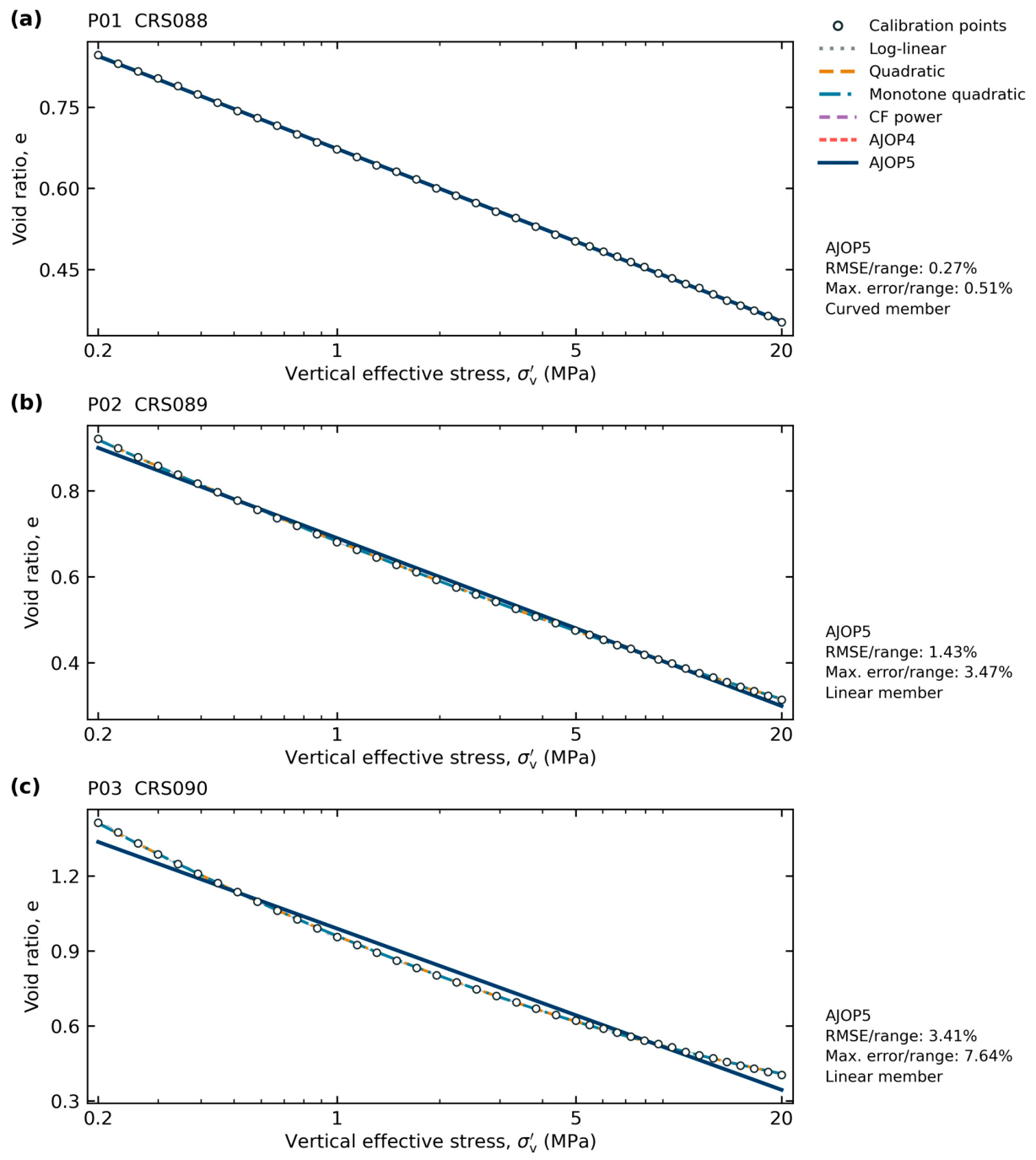
Figure 3.
Complete-window calibration of Reece et al. [54] trajectories P01–P03. Symbols are derived calibration locations; pale traces retain the continuous source records. Every model uses every symbol. Curves that coincide can obscure one another. Side notes report AJOP5 errors relative to the observed void-ratio range; these are approximation diagnostics, not independent predictions.
4.4. Stress Dependence Within the Draupne Specimen
The six reconstructed primary-loading endpoints are listed in Table 3. The interval logarithmic slope rose from 0.00453 over 10.98–15.00 MPa to 0.03161 over 50.63–75.96 MPa, a factor of 6.97. In contrast, the log-strain secant constrained modulus varied from 3.50 to 2.39 GPa. The two statements are compatible because Equation (12) contains effective stress and void ratio: an approximately stable modulus can coexist with a strongly increasing logarithmic slope. This is the central empirical reason not to use the word compressibility without its mathematical definition.
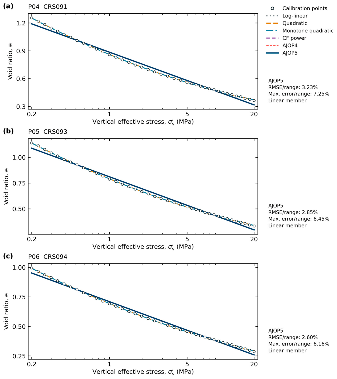
Figure 4.
Complete-window calibration of Reece et al. [54] trajectories P04–P06. AJOP4 and AJOP5 select exact linear members for all three windows. The quadratic follows the concave-up response more closely. Normalized average and maximum AJOP5 errors quantify the approximation left by the line; symbols, traces, and models follow Figure 3.
Using the first and last observed interval slopes as finite-window extrema gives a diagnostic slope ratio of 6.97 and a minimax relative error of 74.9% for one constant slope over those extrema. This is not an estimate of the asymptotic parameters in Equation (13), because the six endpoints do not demonstrate that either asymptote was reached. It is a direct finite-window result. The ratio remained between 6.96 and 6.97 when the endpoint window changed from 30 to 120 min, so the conclusion is not caused by the one-hour endpoint rule.
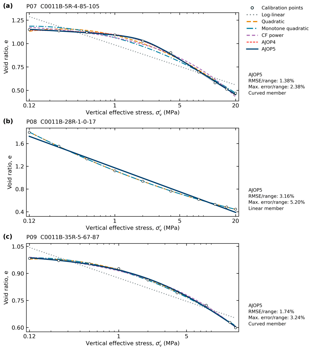
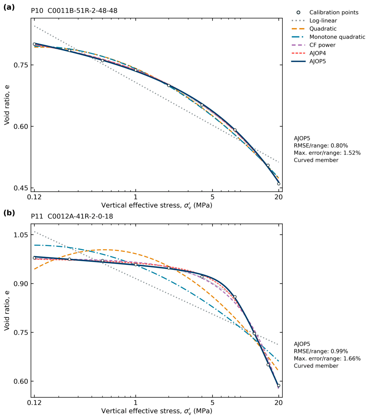
Figure 5.
Complete-window calibration of Hüpers–Kopf [55] incremental-loading trajectories P07–P09. P07 and P09 are natural samples; P08 is remolded. Every plotted source endpoint enters calibration. The positive-curvature P08 window selects a linear AJOP member, whereas P07 and P09 require curvature. The residual panels in S2 show small differences between overlapping curves.
Figure 6.
Complete-window calibration of Hüpers–Kopf [55] natural incremental-loading trajectories P10 and P11. These cases show the benefit of a transition toward a higher compression slope. Unconstrained quadratic curves reverse direction locally, and enforcing monotonicity increases their residuals. Complete-window fits do not establish prediction from the lower-stress subset.
4.5. Draupne Prediction from Five Endpoints
The high-stress holdout distinguishes interpolation from prediction (Table 4 and Figure 9). Calibrated through 50.63 MPa, the constant-log-slope model overpredicted the held-out void ratio by 0.01025. This error equals 79.9% of the observed void-ratio change over the held interval. Constant constrained compressibility reduced the error to 0.00230, or 18.0%, but still exceeded the 10% constitutive screen; the quadratic error was 0.00396, or 30.9%. Within-specimen leave-one-out cross-validation gave RMSE values of 0.005608, 0.001124, and 0.002072 for these three models, respectively, and therefore preserved the same low-order ranking. These cross-validation values do not estimate between-specimen performance. With the transition-stress bound set only from the five training endpoints, the nested transition gave a holdout error of 0.00211, or 16.4%. It also exceeded the 10% screen and had only one residual degree of freedom, so it remains a diagnostic rather than a validated predictor.
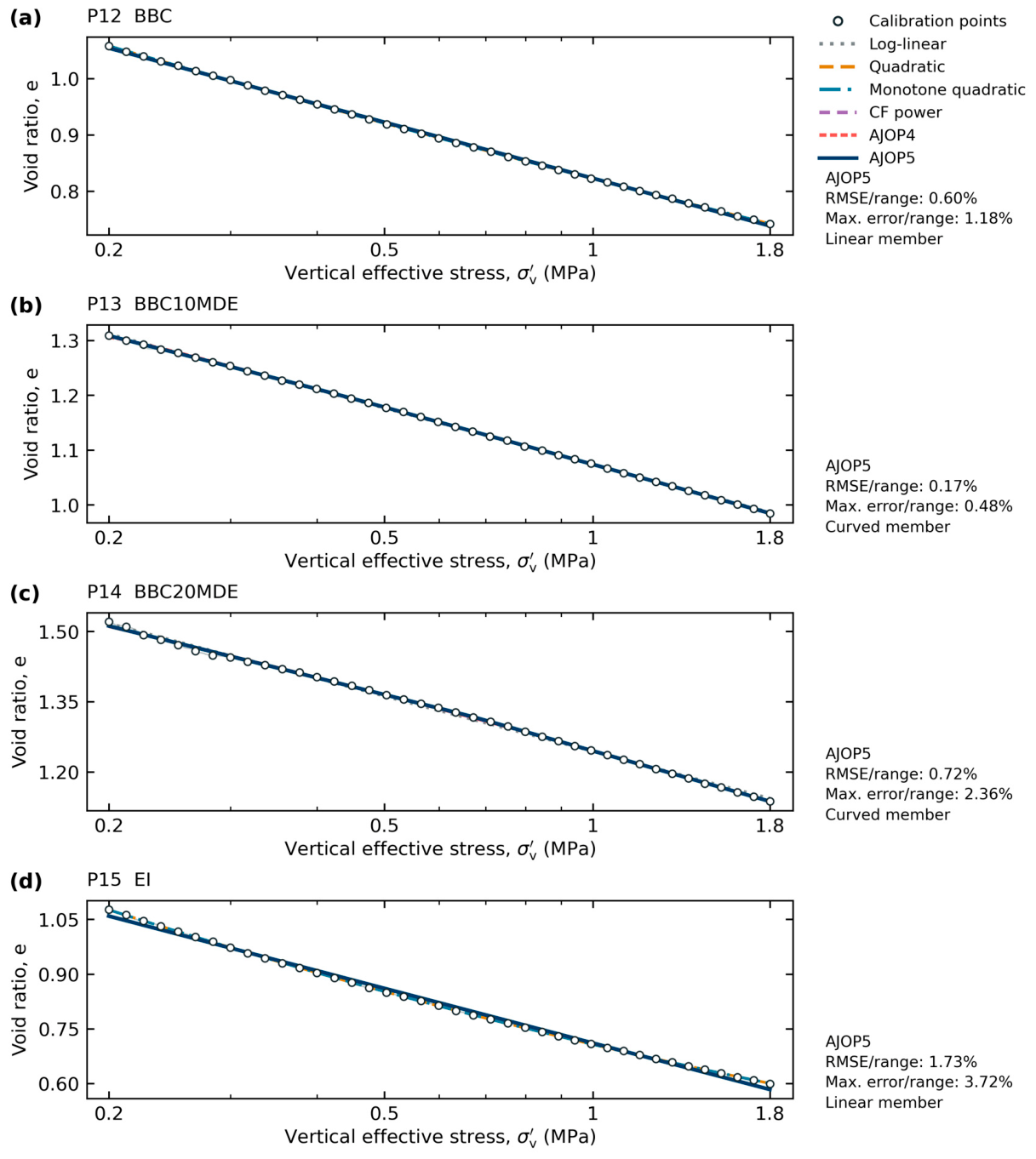
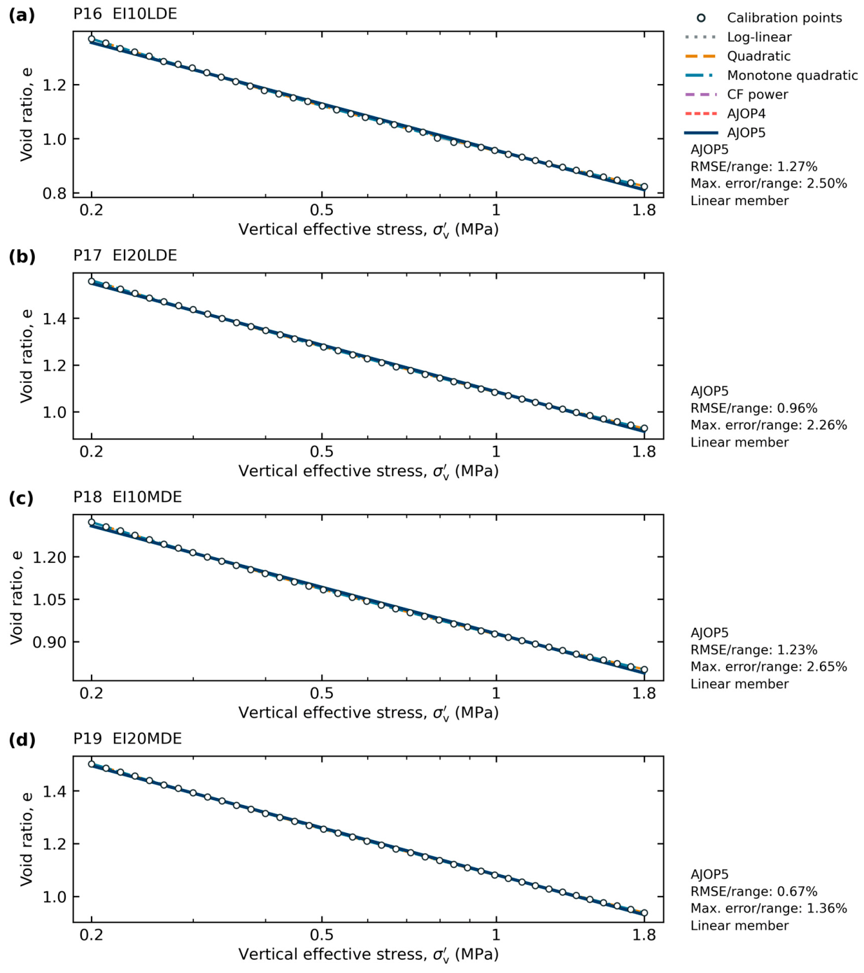
Figure 7.
Complete-window calibration of Scott–Reece [56,57] trajectories P12–P15. BBC denotes Boston Blue Clay, EI denotes Eugene Island sediment, and MDE denotes marine diatomaceous earth; numerals indicate dry-mass percentage addition. P12 and P15 select linear AJOP members, while P13 and P14 retain curvature. All symbols are derived calibration locations.
Figure 8.
Complete-window calibration of Scott–Reece [56,57] trajectories P16–P19. LDE and MDE denote lacustrine and marine diatomaceous earth, respectively. Each AJOP fit selects the linear member over the observed window. The lower quadratic residuals and the remaining AJOP approximation errors are both retained; none of these curves is an independent field prediction.
For the two-parameter models, the all-data constant logarithmic slope was 0.01465 with a nominal 95% interval of 0.00816–0.02113. The constant constrained compressibility was , with an approximate 95% interval of . Expressed per bar, the estimate is , numerically close to the Smeaheia reference value. This numerical proximity does not establish equivalence: constrained compressibility and reservoir pore-volume compressibility have different definitions and stress-path assumptions.
The unrestricted five-parameter fits had smaller in-sample RMSE, but the information needed to interpret them was absent. is undefined for both five-parameter models at when residual variance is counted. A five-point calibration contains no residual degrees of freedom for a five-parameter holdout, so no tail prediction is reported. For the transition law, the scaled sensitivity condition number was , the optimum was 75.96 MPa at the imposed upper boundary, and the nominal profile set extended from 54.19 MPa to that boundary. The profile therefore has no interior upper limit. The Uyeturk–Germaine fit had a scaled condition number of . These diagnostics reject physical interpretation of either five-parameter fit from this specimen alone, even though both interpolate the six endpoints closely.
4.6. Representation and Prediction Across Independent RBBC Specimens
The RBBC cohort addresses variation between independently prepared specimens. Across all 13 endpoints, the quadratic gave the smallest AICc (−88.25) and LOSO RMSE (0.02901). Uyeturk–Germaine gave a lower full-data RMSE of 0.01980, but its scaled sensitivity condition number was , preventing a physical interpretation of its fitted parameters. AJOP selected its exact constant-slope member and returned the same full-data RMSE of 0.02988 as the log-linear relation. This is a valid reduced approximation within the AJOP family; the full cohort does not identify additional transition structure.
The Uyeturk–Germaine relation had the smallest high-stress RMSE, 0.04939, followed by constant logarithmic slope at 0.06069 and the quadratic at 0.07708. Constant constrained compressibility gave 0.81911. The monotone transition fit reached the and bounds in the calibration cohort and produced nonphysical extrapolation, with RMSE 1.70066. The Uyeturk–Germaine relation remained the lowest-error high-stress predictor in the strict- and inclusive cohorts, with RMSE values of 0.03601 and 0.01452, respectively; its condition number nevertheless prevents physical parameter interpretation. Excluding TX1030 in the additional source-audit sensitivity changed the blocked-test ranking: the constant logarithmic slope and collapsed transition law gave RMSE 0.04867, compared with 0.08243 for Uyeturk–Germaine and 0.13714 for the quadratic. The quadratic still minimized AICc. Thus, the primary-cohort holdout advantage of Uyeturk–Germaine is not robust to this exclusion. Independent specimens make the five-parameter holdout admissible, but admissibility does not establish robust prediction or physically interpretable parameters. The framework therefore prevents an attractive in-sample fit or parameterization from being transferred as constitutive evidence when the required prediction and identification tests do not support it.
4.7. Branch Dependence of Intact Mudrock Stiffness
The raw chronology confirms that branch choice is not a minor detail. Endpoint secant moduli were 6.14 GPa for the first unloading, 5.83 GPa for reloading, 8.08 GPa for the high-stress unloading step, and 3.27 and 2.64 GPa for the later unloading stages. These values depend on the selected endpoints and are not identical to tangent moduli reported by Soldal et al. [59], but their ordering shows that one primary-loading parameter cannot represent the complete cycle. The published 3.8–8.3 GPa unloading range was therefore used only as a storage-screening bound.
The result also limits transfer. The Draupne specimen came from the Ling Depression, not Smeaheia, and the stress range of its measured unloading branch lies above the 6–10 MPa effective-stress range used in the reduced-order Smeaheia calculation. It supplies formation-relevant branch information, but it neither calibrates the Smeaheia caprock nor validates Equation (7) for intact mudstone.
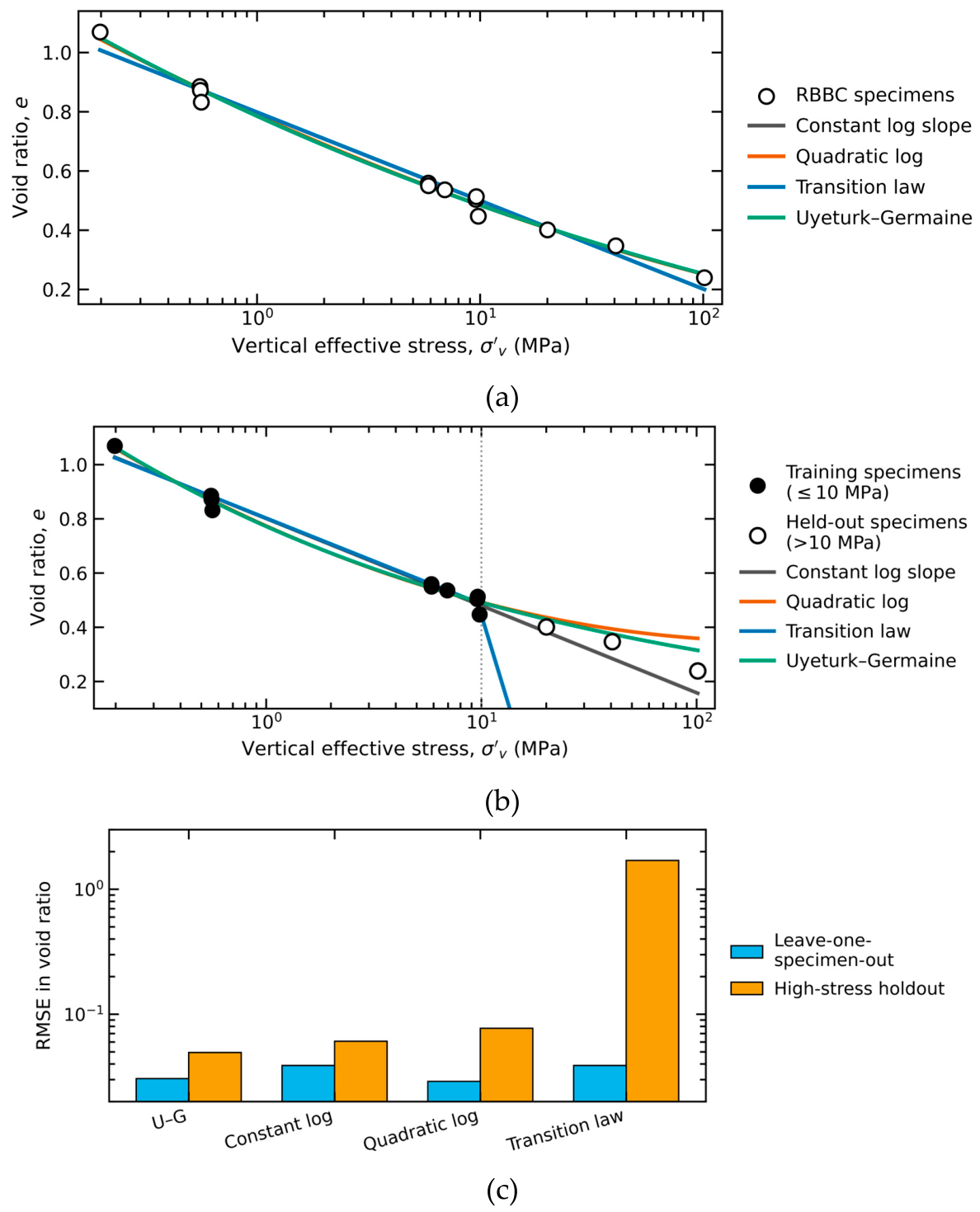
Figure 10.
Independent-specimen RBBC stress test using source-tabulated pre-shear consolidation endpoints. (a) Primary cohort and full-data fits; the monotone transition law collapses to the constant logarithmic slope. (b) Predictions above 10 MPa after calibration on 10 specimens at or below 10 MPa; the transition-law prediction leaves the physical plotting range. Constant constrained compressibility is omitted from the panels because of its larger scale but is reported in Table 5. (c) Leave-one-specimen-out and blocked high-stress RMSE on a logarithmic axis.
4.8. Archival Smeaheia Pressure Classification
Table 6 reconstructs the twelve pressure outcomes in the official Smeaheia report [26,27]. Pressure buildup increased as pore-volume compressibility and connected volume decreased. Across all twelve compressibility–volume combinations, four exceeded the 33 bar pre-fractured-caprock screen and two exceeded the 65 bar intact-caprock screen. Both 65 bar exceedances occurred for the low connected-volume case. For the base connected volume of 160 , the three compressibility assumptions produced 39, 25, and 15 bar after 50 years. The archived property choice therefore spans 24 bar within that geological model, injection case, and connected-volume assumption.
For the base connected volume, reclassification against the updated integrity screens changes the engineering conclusion. The 39 bar case exceeds the conservative 33 bar pre-fractured-caprock screen by 6 bar, whereas the 25 and 15 bar cases remain below it by 8 and 18 bar. All three remain below the 65 bar intact-caprock screen by 26–50 bar. Across the full twelve-case archive, classification depends jointly on pore-volume compressibility and connected volume; the exercise does not identify which input is correct. It does show that the documented property range is large enough to alter a project-specific screening outcome.
4.9. Conditional One-Dimensional Rebound Scale
The stress log gives an initial effective vertical stress of 10.074 MPa at 1260.5 m TVD/KB. Under the , unit-Biot-coefficient and fixed-total-stress end-member, the base-volume pressure rises reduce that value to 6.17, 7.57, and 8.57 MPa for the pessimistic, reference, and optimistic compressibility cases, respectively. Combining the 79–129 m thickness range with gives conditional rebound ranges of 3.7–13.2, 2.4–8.5, and 1.4–5.1 cm (Table 7). For any , these values scale linearly toward zero.
These rebound bounds are conditional one-dimensional estimates, not site predictions of surface movement or caprock deformation. They show the scale introduced by branch-stiffness choice under a stated transmission assumption. The factor between the two unloading-modulus bounds is 2.18, which exceeds the 10% tangent-property screen, but the unknown transmission factor and three-dimensional stress redistribution prevent a site deformation claim. The pressure-screen reclassification in Section 4.8 is therefore the stronger storage consequence, and the main decision conclusion does not depend on the rebound end-member.
4.10. Implications for Compressibility Selection in Storage Assessment
Model complexity should follow the evidence available over the intended operating interval. Akai et al. [65] found that a simple storage-capacity estimate agreed closely with reservoir simulations under selected conditions, while irreversible compaction limited its accuracy in other cases. Lee et al. [33] obtained a nearly linear relation between vertical strain and pore-pressure increase at greater depth in their analytical scenarios, despite stronger nonlinearity at shallower depths. These findings support testing where a simplification is adequate. In the present benchmark, reduced linear AJOP members describe several observed windows; adding transition parameters is useful only where the data resolve their contribution.
For calibration planning, the blocked results identify an information requirement: observations must constrain the branch needed for prediction. Extending a curved segment toward its subsequent linear branch can provide information that additional points within the same early segment cannot. Where this information is absent, the fitted transition parameters should not be transferred as identified properties. The minimax bound offers an exclusion test for a constant logarithmic slope, but passing it does not validate a reservoir compressibility. Application to injection additionally requires unloading data and mechanical constraints appropriate to the target formation.
The importance of the remaining property uncertainty depends on the decision being assessed. Compressibility was not among the five most influential inputs to storage-efficiency uncertainty in the Smeaheia analysis of Wang et al. [28]. The present archive instead asks whether assigned values change a pressure-screen classification at specified connected volumes. These are different outputs under different assessment assumptions; the observed reclassification does not establish a universal sensitivity ranking. It identifies a case in which better-supported compressibility inputs could change screening confidence. Demonstrating improved pressure prediction from AJOP would require site-specific branch calibration and a coupled reservoir comparison.
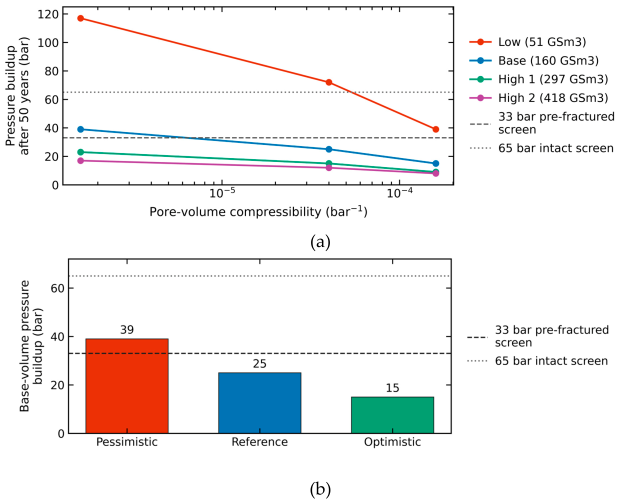
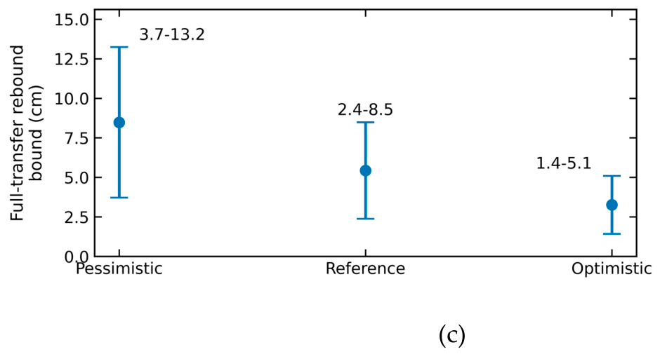
Figure 11.
Smeaheia archival pressure and screening consequences. (a) Pressure buildup reported for three constant pore-volume compressibilities and four connected-volume cases. (b) Base-volume cases compared with the updated 33 bar pre-fractured and 65 bar intact-caprock screens. (c) Conditional rebound range from the 79–129 m thickness and 3.8–8.3 GPa unloading-modulus bounds. Panel (c) scales linearly to zero as decreases and is not a coupled displacement prediction.
5. Discussion and Limitations
The 19-trajectory analysis is an exploratory benchmark assembled from three published sources. The sources were not sampled to represent a statistical population of storage rocks. Fourteen records are resampled from continuous trajectories, and five contain incremental-loading endpoints; their point counts do not measure independent replication. Equal weights apply to the frozen evaluation locations, whose spacing is not uniform after the original training and test grids are combined. Reported counts describe this benchmark and these weights. They do not estimate a probability of success for a new material.
The positive-curvature cases are scientifically relevant. AJOP often approximates them with its linear member, while a quadratic follows their curvature more closely. Reece et al. report stress-dependent changes in compression index associated with sediment composition [54]; Scott and Reece document composition and diatom effects [56]. These observations do not support attributing all concave-up behavior to creep. Time, strain rate, fabric, stress history, and preparation can affect compression [30,37,38,39,40,41,42,43,44,45,46,47,48,50], but the present static fits cannot separate those mechanisms. A creep explanation would require compatible hold-time or rate-dependent evidence and a time-dependent analysis.
The RBBC cohort consists of terminal states from different specimens, so its scatter includes preparation and apparatus effects. Its linear AJOP fit demonstrates representation under the selected objective; the poor blocked AJOP prediction remains a separate adverse result. The Draupne record contains only six loading endpoints from one off-site specimen. Neither its close five-parameter fit nor its boundary profile identifies a transferable transition law. The original porosity reference and strain reconstruction remain explicit. The analytical slope bound applies to the actual extrema over the evaluated interval; observed finite-window slopes do not prove that either asymptote has been reached.
The Smeaheia pressure values are archived outputs, not results of a new three-dimensional simulator run. The reduced-order rebound calculation is conditional on one-dimensional response and an explicit pressure-transmission factor. It does not resolve the full stress tensor, thermal effects, faults, hydraulic breakthrough, surface displacement, or coupled pressure–deformation feedback. The 33 and 65 bar values are project-report screening limits at the stated reference depth, not general regulatory thresholds. Comparing the archived reservoir-pressure increments with these limits is a screening exercise; it does not resolve the spatial caprock pressure or stress field. Because all archived runs use constant compressibilities, they demonstrate sensitivity to the chosen constant, not superiority of a stress-dependent reservoir law. The engineering conclusion rests on reclassification of the archived pressure matrix; it does not require the rebound end-member. Finally, Draupne caprock constrained compressibility and reservoir pore-volume compressibility remain distinct quantities; their numerical proximity does not establish equivalence.
6. Conclusions
Compressibility assumptions for geological CO₂ storage require separate checks of curve approximation, prediction, parameter identification, and engineering consequence. The analytical minimax bound identifies when no constant logarithmic slope can meet a specified relative tolerance over a given interval. A straight compression curve can still have stress-dependent tangent compressibility; its adequacy does not validate a constant reservoir property or transfer between loading branches.
Across 19 complete published trajectories, AJOP5 gave a median range-normalized RMSE of 1.27%, a maximum of 3.41%, and positive monotone curves throughout all observed windows. Twelve fits selected the exact linear member. Fourteen fits were within the illustrative 2% RMSE band and all were within 5%; the largest pointwise error was 7.64%. These results support a common family for linear and curved approximation, subject to purpose-specific tolerances. The quadratic fitted 14 of 19 curves more closely and had a lower median error of 0.26%, but its worst error was 8.81% and four curves reversed compression locally. Enforcing monotonicity removed these reversals but raised its worst error to 12.47%. No model was universally superior.
Calibration must constrain the feature used for prediction. A nearly straight observed window can use a reduced linear AJOP member; a window beginning with curvature needs enough subsequent information to constrain the terminal branch. These principles do not establish an independently validated selection rule. Full-data success does not repair an adverse blocked result, and exploratory slope-guided refits do not supply independent validation. The retained trajectory, RBBC, and Draupne tests expose these prediction and identification limits.
Four of twelve archived Smeaheia scenarios exceeded the 33 bar screen and two exceeded the 65 bar screen. The pressure classifications were sensitive to the assigned constant compressibility and connected volume. This is a decision consequence of the archived assumptions, not evidence that AJOP improves reservoir pressure prediction. Loading envelopes, unloading stiffness, and reservoir pore-volume compressibility retain their separate meanings.
The practical contribution is an assessment sequence: specify the property, stress window, and path; quantify approximation and tangent errors; test prediction separately; and carry unresolved property uncertainty into the storage screen. The expanded evidence supports useful linear and nonlinear AJOP approximations across the tested responses, while making explicit the additional calibration and field evidence needed for engineering use.
Supplementary Materials
The following supporting information can be downloaded at the website of this paper posted on Preprints.org. File S1 contains the v20 reproducibility package, complete numerical tables, editable figure sources, earlier frozen analyses, verification scripts, source register, and SHA-256 manifest. File S2 contains all 127 analysis figures grouped by purpose and provenance, with full-data calibration separated from prediction and exploratory refits.
Author Contributions
Conceptualization, N.K. and T.C.; methodology, N.K. and T.C.; software, N.C., N.K. and T.C.; validation, N.K., A.K. and S.E.; formal analysis, N.K. and T.C.; investigation, N.C., T.C., S.I., A.K. and S.S.; resources, N.C., S.I. and S.S.; data curation, N.C., T.C. and S.I.; writing—original draft preparation, N.K. and T.C.; writing—review and editing, N.K., A.K., S.E. and S.S.; visualization, N.C., N.K. and S.E.; supervision, S.I., A.K., S.E. and S.S.; project administration, N.K.; funding acquisition, N.K. All authors have read and agreed to the published version of the manuscript.
Funding
This research project was financially supported by Mahasarakham University.
Institutional Review Board Statement
Not applicable.
Informed Consent Statement
Not applicable.
Data Availability Statement
The Reece et al. and Hüpers–Kopf source workbooks accompany their IODP reports [54,55]. The Scott–Reece workbook is archived on Zenodo, version 2 [57]. The Casey thesis is available from MIT [58], the Draupne laboratory files from DataverseNO [60], and the Smeaheia packages from CO₂DataShare [26]. Supplementary File S1 contains the extracted analysis records, source URLs and hashes, exact transformations, cohort flags, parameters, predictions, and figure scripts. Copyrighted source papers and the Casey thesis PDF are not redistributed. The Smeaheia pressures remain identified as archived outputs.
Conflicts of Interest
The authors declare no conflicts of interest.
Declaration of Generative AI and AI-Assisted Technologies in the Writing Process
During the preparation of this work, the authors used Claude (Anthropic) and ChatGPT (OpenAI) to assist with manuscript editing and language refinement and with drafting scripts for figure preparation and numerical cross-checking. All scientific content, mathematical formulations, calculations, results, interpretations, and conclusions were independently developed, reviewed, and verified by the authors. The authors subsequently reviewed and edited all AI-assisted content and take full responsibility for the content of the published article.
References
- IPCC. Climate Change 2022: Mitigation of Climate Change; Cambridge University Press: Cambridge, UK, 2022. [Google Scholar] [CrossRef]
- Bui, M.; Adjiman, C.S.; Bardow, A.; Anthony, E.J.; Boston, A.; Brown, S.; Fennell, P.S.; Fuss, S.; Galindo, A.; Hackett, L.A.; et al. Carbon capture and storage (CCS): The way forward. Energy Environ. Sci. 2018, 11, 1062–1176. [Google Scholar] [CrossRef]
- Bachu, S. CO₂ storage in geological media: Role, means, status and barriers to deployment. Prog. Energy Combust. Sci. 2008, 34, 254–273. [Google Scholar] [CrossRef]
- Benson, S.M.; Cole, D.R. CO₂ sequestration in deep sedimentary formations. Elements 2008, 4, 325–331. [Google Scholar] [CrossRef]
- Ringrose, P.S.; Meckel, T.A. Maturing global CO₂ storage resources on offshore continental margins to achieve 2DS emissions reductions. Sci. Rep. 2019, 9, 17944. [Google Scholar] [CrossRef] [PubMed]
- Szulczewski, M.L.; MacMinn, C.W.; Herzog, H.J.; Juanes, R. Lifetime of carbon capture and storage as a climate-change mitigation technology. Proc. Natl. Acad. Sci. USA 2012, 109, 5185–5189. [Google Scholar] [CrossRef] [PubMed]
- Biot, M.A. General theory of three-dimensional consolidation. J. Appl. Phys. 1941, 12, 155–164. [Google Scholar] [CrossRef]
- Biot, M.A.; Willis, D.G. The elastic coefficients of the theory of consolidation. J. Appl. Mech. 1957, 24, 594–601. [Google Scholar] [CrossRef]
- Nur, A.; Byerlee, J.D. An exact effective stress law for elastic deformation of rock with fluids. J. Geophys. Res. 1971, 76, 6414–6419. [Google Scholar] [CrossRef]
- Rutqvist, J. The geomechanics of CO₂ storage in deep sedimentary formations. Geotech. Geol. Eng. 2012, 30, 525–551. [Google Scholar] [CrossRef]
- Streit, J.E.; Hillis, R.R. Estimating fault stability and sustainable fluid pressures for underground storage of CO₂ in porous rock. Energy 2004, 29, 1445–1456. [Google Scholar] [CrossRef]
- Hawkes, C.D.; McLellan, P.J.; Bachu, S. Geomechanical factors affecting geological storage of CO₂ in depleted oil and gas reservoirs. J. Can. Pet. Technol. 2005, 44, 52–61. [Google Scholar] [CrossRef]
- Birkholzer, J.T.; Zhou, Q. Basin-scale hydrogeologic impacts of CO₂ storage: Capacity and regulatory implications. Int. J. Greenh. Gas Control 2009, 3, 745–756. [Google Scholar] [CrossRef]
- Rutqvist, J.; Birkholzer, J.T.; Tsang, C.F. Coupled reservoir–geomechanical analysis of the potential for tensile and shear failure associated with CO₂ injection in multilayered reservoir–caprock systems. Int. J. Rock Mech. Min. Sci. 2008, 45, 132–143. [Google Scholar] [CrossRef]
- Rutqvist, J.; Vasco, D.W.; Myer, L. Coupled reservoir–geomechanical analysis of CO₂ injection and ground deformations at In Salah, Algeria. Int. J. Greenh. Gas Control 2010, 4, 225–230. [Google Scholar] [CrossRef]
- Thompson, N.; Andrews, J.S.; Bjørnarå, T.I. Assessing potential thermo-mechanical impacts on caprock due to CO₂ injection—A case study from Northern Lights CCS. Energies 2021, 14, 5054. [Google Scholar] [CrossRef]
- Zheng, X.; Espinoza, D.N. Measurement of unloading pore volume compressibility of Frio sand under uniaxial strain stress path and implications on reservoir pressure management. Rock Mech. Rock Eng. 2021, 54, 5745–5760. [Google Scholar] [CrossRef]
- Vasco, D.W.; Rucci, A.; Ferretti, A.; Novali, F.; Bissell, R.C.; Ringrose, P.S.; Mathieson, A.S.; Wright, I.W. Satellite-based measurements of surface deformation reveal fluid flow associated with the geological storage of carbon dioxide. Geophys. Res. Lett. 2010, 37, L03303. [Google Scholar] [CrossRef]
- White, J.A.; Chiaramonte, L.; Ezzedine, S.; Foxall, W.; Hao, Y.; Ramirez, A.; McNab, W. Geomechanical behavior of the reservoir and caprock system at the In Salah CO₂ storage project. Proc. Natl. Acad. Sci. USA 2014, 111, 8747–8752. [Google Scholar] [CrossRef] [PubMed]
- Verdon, J.P.; Kendall, J.-M.; Stork, A.L.; Chadwick, R.A.; White, D.J.; Bissell, R.C. Comparison of geomechanical deformation induced by megatonne-scale CO₂ storage at Sleipner, Weyburn, and In Salah. Proc. Natl. Acad. Sci. USA 2013, 110, E2762–E2771. [Google Scholar] [CrossRef] [PubMed]
- Zoback, M.D.; Gorelick, S.M. Earthquake triggering and large-scale geologic storage of carbon dioxide. Proc. Natl. Acad. Sci. USA 2012, 109, 10164–10168. [Google Scholar] [CrossRef] [PubMed]
- Vilarrasa, V.; Carrera, J. Geologic carbon storage is unlikely to trigger large earthquakes and reactivate faults through which CO₂ could leak. Proc. Natl. Acad. Sci. USA 2015, 112, 5938–5943. [Google Scholar] [CrossRef] [PubMed]
- Cappa, F.; Rutqvist, J. Impact of CO₂ geological sequestration on the nucleation of earthquakes. Geophys. Res. Lett. 2011, 38, L17313. [Google Scholar] [CrossRef]
- Shchipanov, A.; Kollbotn, L.; Encinas, M.; Fjelde, I.; Berenblyum, R. Periodic CO₂ injection for improved storage capacity and pressure management under intermittent CO₂ supply. Energies 2022, 15, 566. [Google Scholar] [CrossRef]
- Rahman, M.J.; Fawad, M.; Mondol, N.H. 3D field-scale geomechanical modeling of potential CO₂ storage site Smeaheia, offshore Norway. Energies 2022, 15, 1407. [Google Scholar] [CrossRef]
- Gassnova. Smeaheia CO₂ Storage Prospect Reference Dataset; NIRD RDA, 2021; Version 1. [CrossRef]
- Erichsen, E.; Rørvik, K.-L.; Haaberg, K.; Keaney, G. Troll Kystnær—Subsurface Status Report; Document TL02-ROS-Z-RA-0005, Revision 03; ROSS Offshore, 2012; pp. 46, 51, 56, 62–63. Available online: https://ccsnorway.com/app/uploads/sites/6/2019/09/tl02-ros-z-ra-0005-troll-kystnaer-subsurface-status-report-rev03.pdf (accessed on 10 October 2026).
- Wang, Z.; Qi, S.; Zheng, B. Uncertainty analysis of the storage efficiency factor for CO₂ saline resource estimation. Energies 2024, 17, 1297. [Google Scholar] [CrossRef]
- Lee, S.-Y.; Mohamed, F.R.; Lee, K.-H.; McPherson, B.; Balch, R.; Yoon, S. Probabilistic evaluation of geomechanical risks in CO₂ storage: An exploration of caprock integrity metrics using a multilaminate model. Energies 2023, 16, 6954. [Google Scholar] [CrossRef]
- Nowakowski, A. The influence of rate of change in confining and pore pressure on values of the modulus of compressibility of the rock skeleton and Biot’s coefficient. Energies 2021, 14, 3056. [Google Scholar] [CrossRef]
- Giani, G.; Orsatti, S.; Peter, C.; Rocca, V. A coupled fluid flow–geomechanical approach for subsidence numerical simulation. Energies 2018, 11, 1804. [Google Scholar] [CrossRef]
- Wei, C.; Wang, L.; Li, B.; Xiong, L.; Liu, S.; Zheng, J.; Hu, S.; Song, H. A study of nonlinear elasticity effects on permeability of stress sensitive shale rocks using an improved coupled flow and geomechanics model: A case study of the Longmaxi Shale in China. Energies 2018, 11, 329. [Google Scholar] [CrossRef]
- Lee, Y.; Song, I.; Park, C. Analytical assessment of CO₂-storage efficiency and geomechanical-coupling behaviors using poromechanical experiments. Int. J. Rock Mech. Min. Sci. 2025, 196, 106320. [Google Scholar] [CrossRef]
- Chen, M.; Lai, Z.; Kang, Y.; Fang, S.; Liu, H.; Wang, W.; Shen, J.; Chen, Z. Investigation of stress sensitivity of shale nanopores via a nuclear magnetic resonance method. Energies 2023, 16, 138. [Google Scholar] [CrossRef]
- Yao, L.; Lei, Q.; Yang, Z.; He, Y.; Li, H.; Zhao, G.; Zheng, Z.; Hou, H.; Du, M.; Cheng, L. Online nuclear magnetic resonance analysis of the effect of stress changes on the porosity and permeability of shale oil reservoirs. Energies 2023, 16, 1139. [Google Scholar] [CrossRef]
- Qiu, X.; Liu, H.; Liu, M.; Mao, H.; Wang, D.; Ying, Q.; Ban, S. Pore structure evolution in sandstone of underground gas storage during cyclic injection and production based on nuclear magnetic resonance technology. Energies 2023, 16, 2096. [Google Scholar] [CrossRef]
- Skempton, A.W. The consolidation of clays by gravitational compaction. Q. J. Geol. Soc. 1969, 125, 373–411. [Google Scholar] [CrossRef]
- Olson, R.E.; Mesri, G. Mechanisms controlling compressibility of clays. J. Soil Mech. Found. Div. 1970, 96, 1863–1878. [Google Scholar] [CrossRef]
- Burland, J.B. On the compressibility and shear strength of natural clays. Géotechnique 1990, 40, 329–378. [Google Scholar] [CrossRef]
- Vasseur, G.; Djeran-Maigre, I.; Grunberger, D.; Rousset, G.; Tessier, D.; Velde, B. Evolution of structural and physical parameters of clays during experimental compaction. Mar. Pet. Geol. 1995, 12, 941–954. [Google Scholar] [CrossRef]
- Dewhurst, D.N.; Aplin, A.C.; Sarda, J.-P.; Yang, Y. Compaction-driven evolution of porosity and permeability in natural mudstones: An experimental study. J. Geophys. Res. Solid Earth 1998, 103, 651–661. [Google Scholar] [CrossRef]
- Mondol, N.H.; Bjørlykke, K.; Jahren, J.; Høeg, K. Experimental mechanical compaction of clay mineral aggregates—Changes in physical properties of mudstones during burial. Mar. Pet. Geol. 2007, 24, 289–311. [Google Scholar] [CrossRef]
- Yang, Y.; Aplin, A.C. A permeability–porosity relationship for mudstones. Mar. Pet. Geol. 2010, 27, 1692–1697. [Google Scholar] [CrossRef]
- Casey, B.; Germaine, J.T.; Flemings, P.B.; Fahy, B.P. Estimating horizontal stresses for mudrocks under one-dimensional compression. Mar. Pet. Geol. 2015, 65, 178–186. [Google Scholar] [CrossRef]
- Casey, B.; Reece, J.S.; Germaine, J.T. One-dimensional normal compression laws for resedimented mudrocks. Mar. Pet. Geol. 2019, 103, 397–403. [Google Scholar] [CrossRef]
- Dessouki, M.; Hathon, L.; Myers, M. Permeability and porosity modelling for resedimented mudrocks—Applications for compaction dominated mudrock systems. Mar. Pet. Geol. 2021, 128, 104945. [Google Scholar] [CrossRef]
- Uyeturk, C.E.; Germaine, J.T. A general model for the compression of mudrocks. Mar. Pet. Geol. 2025, 174, 107327. [Google Scholar] [CrossRef]
- Uyeturk, C.E.; Germaine, J.T.; Plumb, R. Laboratory characterization of secondary compression behavior of three mudrocks from 1 to 100 MPa effective stress. Geotech. Test. J. 2025, 48, 942–955. [Google Scholar] [CrossRef]
- Kaewhanam, N.; Chaimoon, K. A simplified silty sand model. Appl. Sci. 2023, 13, 8241. [Google Scholar] [CrossRef]
- Phonchamni, N.; Chatwong, T.; Udomchai, A.; Sultornsanee, S.; Angkawisittpan, N.; Sangiamsak, N.; Kaewhanam, N. Refined consolidation settlement calculation based on the oedometer tests for normally and overconsolidated clays. Appl. Sci. 2025, 15, 5777. [Google Scholar] [CrossRef]
- Chatwong, T.; Kaewhanam, N.; Kampala, A.; Eua-apiwatch, S.; Sultornsanee, S. AJOP-T: A high-order hardening law for continuous teardrop bounding surface plasticity. Mathematics 2026, 14, 2975. [Google Scholar] [CrossRef]
- Bhandari, A.R.; Ewy, R.T.; Flemings, P.B.; Germaine, J.T. Comparing compression and shear behavior of intact and resedimented mudrock to illuminate the rheology of mudrocks. In Proceedings of the 58th U.S. Rock Mechanics/Geomechanics Symposium, Golden, CO, USA, 23–26 June 2024; Paper ARMA-2024-1042. [Google Scholar] [CrossRef]
- Karig, D.E.; Ask, M.V.S. Geological perspectives on consolidation of clay-rich marine sediments. J. Geophys. Res. Solid Earth 2003, 108, 2197. [Google Scholar] [CrossRef]
- Reece, J.S.; Flemings, P.B.; Germaine, J.T. Data report: permeability, compressibility, and microstructure of resedimented mudstone from IODP Expedition 322, Site C0011. Proc. IODP 2013, 322. [Google Scholar] [CrossRef]
- Hüpers, A.; Kopf, A.J. Data report: consolidation properties of silty claystones and sandstones sampled seaward of the Nankai Trough subduction zone, IODP Sites C0011 and C0012. Proc. IODP 2012, 322. [Google Scholar] [CrossRef]
- Scott, W.; Reece, J.S. The influence of diatoms on hydromechanical properties of marine sediments. Geochem. Geophys. Geosyst. 2025, 26, e2024GC012064. [Google Scholar] [CrossRef]
- Scott, W.; Reece, J.S. The Influence of Diatoms on Hydromechanical Properties of Marine Sediments; Version 2; Zenodo, 2024. [Google Scholar] [CrossRef]
- Casey, B. The Consolidation and Strength Behavior of Mechanically Compressed Fine-Grained Sediments. Ph.D. Thesis, Massachusetts Institute of Technology, Cambridge, MA, USA, 2014. Available online: https://hdl.handle.net/1721.1/90039 (accessed on 10 October 2026).
- Soldal, M.; Skurtveit, E.; Choi, J.C. Laboratory evaluation of mechanical properties of Draupne shale relevant for CO₂ seal integrity. Geosciences 2021, 11, 244. [Google Scholar] [CrossRef]
- Soldal, M. Replication Data for: Laboratory Evaluation of Mechanical Properties of Draupne Shale Relevant for CO₂ Seal Integrity; DataverseNO, 2023; Volume V1. [Google Scholar] [CrossRef]
- Hurvich, C.M.; Tsai, C.-L. Regression and time series model selection in small samples. Biometrika 1989, 76, 297–307. [Google Scholar] [CrossRef]
- Raue, A.; Kreutz, C.; Maiwald, T.; Bachmann, J.; Schilling, M.; Klingmüller, U.; Timmer, J. Structural and practical identifiability analysis of partially observed dynamical models by exploiting the profile likelihood. Bioinformatics 2009, 25, 1923–1929. [Google Scholar] [CrossRef] [PubMed]
- Shi, Z.; Driba, D.L.; Lopez Rivera, N.; Kariminasab, M.; Beckingham, L.E. A review of coupled geochemical–geomechanical impacts in subsurface CO₂, H₂, and air storage systems. Energies 2024, 17, 2928. [Google Scholar] [CrossRef]
- Schwarz, G. Estimating the dimension of a model. Ann. Stat. 1978, 6, 461–464. [Google Scholar] [CrossRef]
- Akai, T.; Saito, N.; Hiyama, M.; Okabe, H. Numerical modelling on CO₂ storage capacity in depleted gas reservoirs. Energies 2021, 14, 3978. [Google Scholar] [CrossRef]
Figure 1.
Conceptual propagation of a compressibility assumption through a geological CO₂-storage assessment. (a) Injection raises pore pressure in the storage formation and changes the effective-stress path in the reservoir and caprock. (b) Burial is represented as primary loading, whereas pore-pressure increase at approximately fixed total stress produces unloading; the transition band belongs to the loading envelope and is not used as an unloading law. (c) The constitutive relation supplies tangent quantities to the coupled model, which propagates them to pressure, deformation, and integrity outputs. The figure is conceptual and contains no Smeaheia simulation result.
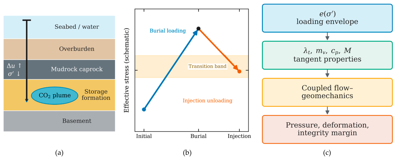
Figure 2.
Dataset-independent consequences of Equations (8), (10), (13), and (14). (a) Normalized local-slope transition versus normalized effective stress for three transition-width parameters; the shaded interval is the exact 10–90% band for . (b) Unavoidable minimax relative error of a constant slope as a function of the asymptotic slope ratio ; the dashed lines mark a 10% tolerance and its critical ratio . The figure contains analytical results only and no fitted data.
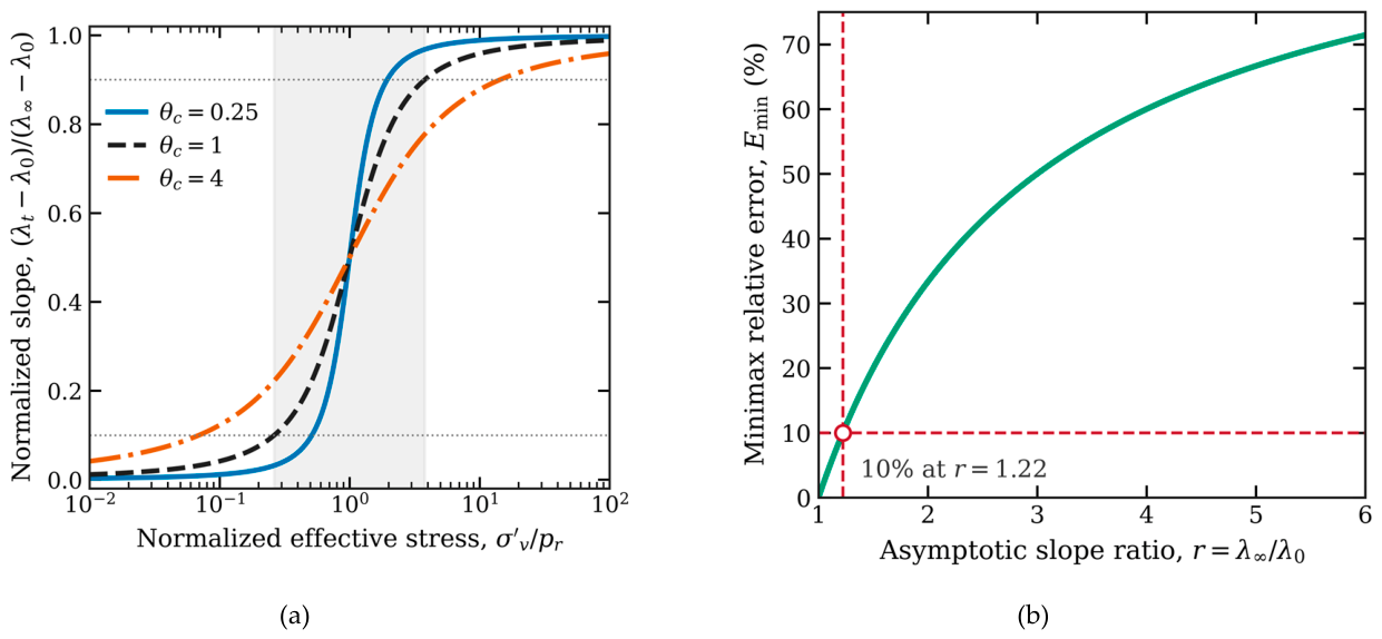
Figure 9.
Reprocessed Draupne oedometer evidence. (a) Stable endpoints with loading, unloading, and reloading kept separate. (b) High-stress prediction after fitting only the first five primary-loading endpoints; the 75.96 MPa point is held out. (c) Profile-likelihood diagnostic for transition stress . The minimum occurs at the upper data boundary, and the nominal 95% set is one-sided. Panel (c) is diagnostic because the full fit has one residual degree of freedom.
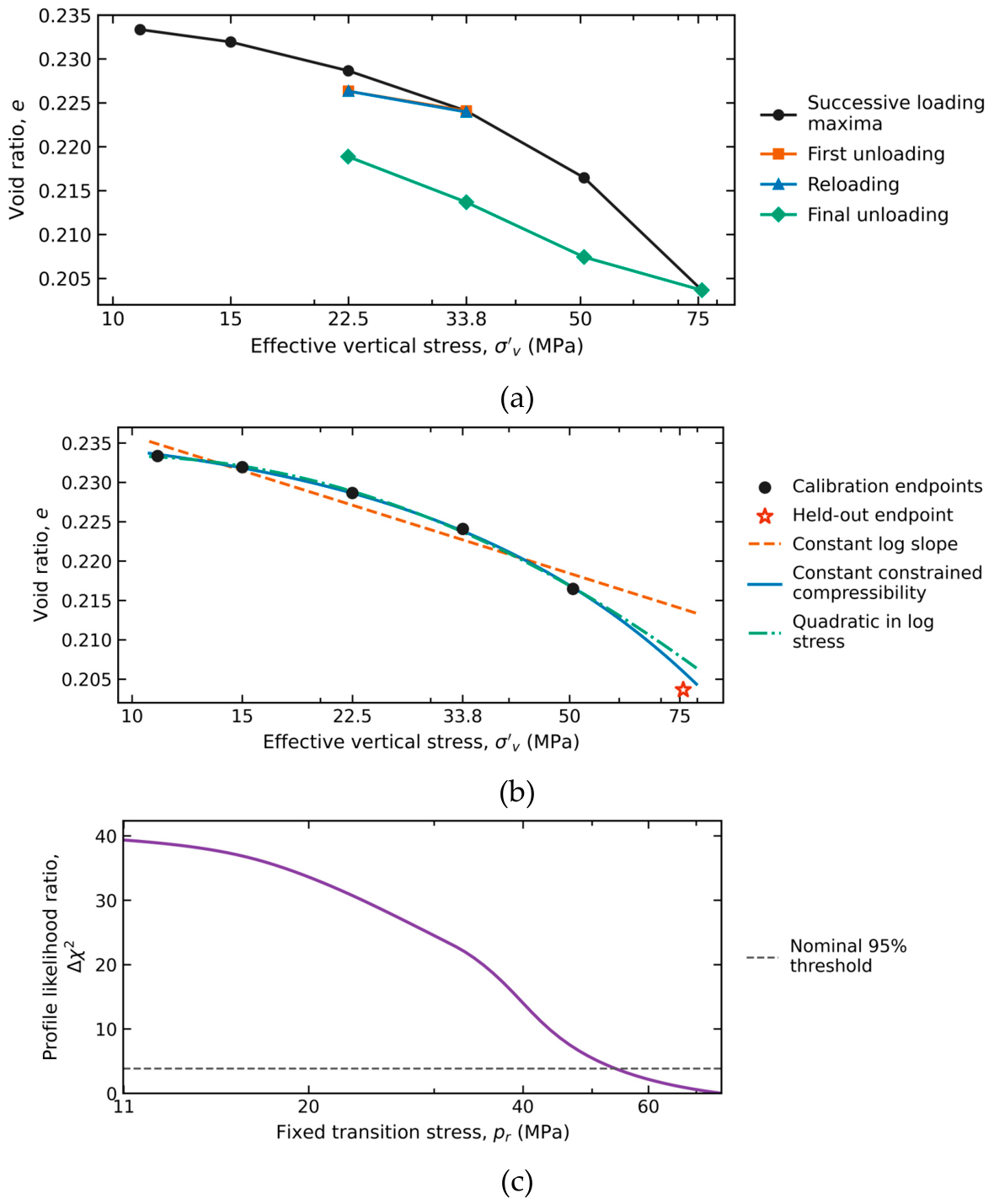

Table 1.
Separate criteria for representation, prediction, identification, and transfer.
| Level | Quantity | Evaluation criterion |
| Representation | Complete-window void ratio | Report RMSE and maximum absolute error relative to the observed range. Compare 1%, 2%, and 5% RMSE bands as descriptive sensitivity levels. Verify positivity and monotonicity. |
| Prediction | , flag error above 10% of the observed held-interval change. For a slope approximation, test the maximum relative slope error over the specified interval. Report absolute error and processing sensitivity. | |
| Identification | and nonlinear parameters | indicates inadequate information for that criterion; it does not alone prove non-identification. |
| Tangent property | Flag a maximum relative difference above 10% over the stated path; retain the physical definition. | |
| Engineering | Pressure or integrity margin | Flag a decision as non-robust when the documented property range changes the 33 or 65 bar Smeaheia classification. |
| Transfer | Material state and branch | Do not transfer primary-loading or off-site values without an explicit sensitivity bound. |
Normalization by the observed range supports within-curve comparison but does not measure relative error in void ratio, stress, settlement, or stiffness. The tangent-property screening tolerance likewise is not a regulatory threshold.
Table 2.
Full-window representation across all 19 trajectories. Errors are percentages of each observed void-ratio range.
Table 2.
Full-window representation across all 19 trajectories. Errors are percentages of each observed void-ratio range.
| Model | Median RMSE (%) | Worst RMSE (%) | ≤ 1% | ≤ 2% | ≤ 5% | Monotone curves |
| Log-linear | 1.73 | 18.88 | 5 | 10 | 15 | 19/19 |
| Quadratic | 0.26 | 8.81 | 15 | 16 | 18 | 15/19 |
| Monotone quadratic | 0.26 | 12.47 | 15 | 16 | 18 | 19/19 |
| CF power | 1.43 | 4.12 | 7 | 12 | 19 | 19/19 |
| AJOP4 | 1.43 | 3.41 | 7 | 14 | 19 | 19/19 |
| AJOP5 | 1.27 | 3.41 | 8 | 14 | 19 | 19/19 |
Counts refer to illustrative RMSE bands, not acceptance certification. All six models were positive over every fitted interval. Monotonicity concerns the continuous fitted curve within that interval.
Table 3.
Reprocessed Draupne primary-loading endpoints and interval properties. and refer to the interval ending at each row.
Table 3.
Reprocessed Draupne primary-loading endpoints and interval properties. and refer to the interval ending at each row.
| (MPa) | (GPa) | ||
|---|---|---|---|
| 10.98 | 0.23335 | — | — |
| 15.00 | 0.23194 | 0.00453 | 3.50 |
| 22.49 | 0.22865 | 0.00811 | 2.81 |
| 33.76 | 0.22408 | 0.01125 | 3.02 |
| 50.63 | 0.21647 | 0.01877 | 2.71 |
| 75.96 | 0.20365 | 0.03161 | 2.39 |
Endpoints are medians of the final 60 min of each hold.
uses logarithmic strain from Equation (4).
Table 4.
Draupne model comparison and 75.96 MPa tail holdout.
| Model | Tail error (%) | Status | ||||
|---|---|---|---|---|---|---|
| Constant log slope | 2 | 0.00313 | −51.19 | 0.01025 | 79.9 | Estimable |
| Constant constrained compressibility | 2 | 0.00053 | −72.59 | 0.00230 | 18.0 | Estimable |
| Quadratic in log stress | 3 | 0.00068 | −39.48 | 0.00396 | 30.9 | Estimable |
| Nested transition | 4 | 0.00010 | — | 0.00211 | 16.4 | One residual df |
| Full transition | 5 | 0.00009 | — | — | — | Holdout inadmissible |
| Uyeturk–Germaine | 5 | 0.00013 | — | — | — | Holdout inadmissible |
Tail error is |prediction − observation| divided by the observed void-ratio change from 50.63 to 75.96 MPa. is undefined where .
Table 5.
Independent-specimen RBBC model comparison and blocked high-stress prediction.
| Model | Diagnostic | |||||
|---|---|---|---|---|---|---|
| Constant log slope | 2 | 0.02988 | −82.61 | 0.03885 | 0.06069 | Estimable |
| 2 | 0.16871 | −37.60 | 0.25783 | 0.81911 | Poor prediction | |
| Quadratic log | 3 | 0.02036 | −88.25 | 0.02901 | 0.07708 | and LOSO |
| Monotone transition | 5 | 0.02988 | — | 0.03885 | 1.70066 | Boundary-limited |
| Uyeturk–Germaine | 5 | 0.01980 | −75.98 | 0.03051 | 0.04939 | Ill-conditioned |
Primary cohort: 13 independent normally consolidated RBBC specimens; calibration at and test at . counts the residual variance as a parameter. The entry is suppressed for the singular transition fit; S1 retains its nominal score for transparency. LOSO denotes leave-one-specimen-out, with each fold initialized from its training data only. The transition-law training fit reached the and bounds and extrapolated outside the physical void-ratio range.
| ) | ||||
|---|---|---|---|---|
| 117 | 39 | 23 | 17 | |
| 72 | 25 | 15 | 12 | |
| 39 | 15 | 9 | 8 |
Values are pressure buildup in bar. The original report scaled the base simulation to alternative connected volumes.
Table 7.
Base-volume Smeaheia integrity margins and conditional full-transmission rebound bounds.
| case | (bar) | (MPa) | (cm) | Margin to 33 bar | Margin to 65 bar |
|---|---|---|---|---|---|
| Pessimistic | 39 | 6.17 | 3.7–13.2 | −6 | 26 |
| Reference | 25 | 7.57 | 2.4–8.5 | 8 | 40 |
| Optimistic | 15 | 8.57 | 1.4–5.1 | 18 | 50 |
Positive pressure margin denotes a value below the screen. is an unknown pressure-transmission factor with . The table assumes unit Biot coefficient and fixed total vertical stress; rebound is a first-order constrained estimate.
Disclaimer/Publisher’s Note: The statements, opinions and data contained in all publications are solely those of the individual author(s) and contributor(s) and not of MDPI and/or the editor(s). MDPI and/or the editor(s) disclaim responsibility for any injury to people or property resulting from any ideas, methods, instructions or products referred to in the content. |
© 2026 by the authors. Licensee MDPI, Basel, Switzerland. This article is an open access article distributed under the terms and conditions of the Creative Commons Attribution (CC BY) license (http://creativecommons.org/licenses/by/4.0/).
Copyright: This open access article is published under a Creative Commons CC BY 4.0 license, which permit the free download, distribution, and reuse, provided that the author and preprint are cited in any reuse.