

Submitted:
15 October 2026
Posted:
16 October 2026
You are already at the latest version
Abstract
Fine particulate matter (PM2.5) is among the most harmful air pollutants, and its costs reach well beyond public health into economic and urban development. This study predicts annual PM2.5 concentrations from climatic, socio-economic, sustainable-development, environmental-perception and technological indicators, using statistical and machine learning methods. The dataset covers ten cities in Europe and Central Asia over 2020–2025 and contains 59 usable country-year observations with eleven explanatory variables. Six predictive models—Linear Regression, Extra Trees, Random Forest, XGBoost, Gradient Boosting, and HistGradientBoosting—were evaluated using five-fold cross-validation and mean absolute error (MAE), root mean square error (RMSE), and coefficient of determination (R²). Linear Regression performed best overall, with the lowest RMSE and the highest R², while Extra Trees produced the lowest MAE. The selected Linear Regression model was fitted to all 59 observations and used to estimate annual PM2.5 concentrations and conduct comparative country-level analysis. SHAP-based interpretation was applied to examine individual predictor contributions. The results suggest that development-related indicators add useful information to meteorological data in air quality assessment. With only 59 observations, however, the findings are exploratory and need to be checked on larger datasets.
Keywords:
air pollution
; PM2.5
; machine learning
; explainable artificial intelligence
; SHAP
; environmental risk
; economic development
; sustainable development
1. Introduction
Air pollution is one of the most serious environmental problems in the world, with conse-quences for public health, economic productivity and urban development. Among various air pollutants, fine particulate matter with a diameter of less than 2.5 μm (PM2.5) is con-sidered one of the most harmful pollutants because it can penetrate deeply into the human respiratory system and cause serious health problems [4]. High levels of PM2.5 are associ-ated with respiratory and cardiovascular diseases, reduced quality of life, and significant socio-economic losses [22]. The formation and distribution of PM2.5 are influenced by multiple interrelated factors, including meteorological conditions, emission sources, ur-banization, economic activity, and environmental management policies [22]. Air quality assessment has traditionally relied on monitoring pollutant concentrations and on look-ing at environmental factors one at a time. This leaves open how PM2.5 relates to the wid-er socio-economic, sustainable-development and technological profile of a country [8]
Machine learning has opened up new ways of assessing and forecasting air quality. Its main advantage here is that it can handle many variables at once and pick up patterns that are hard to see in multidimensional data. Tree-based ensembles and regression mod-els in particular are now widely used to relate pollutant concentrations to sets of explana-tory variables [9,22].
Most of this work, however, uses meteorological variables and direct pollution sources as predictors. Much less is known about whether economic development, progress on sus-tainable development, perceived pollution or national technological readiness add any-thing to the explanation of PM2.5 levels [8,9,24]. Models that draw on such indicators could be especially useful in countries and regions where monitoring networks are sparse and air quality data are hard to obtain [23].
This study asks whether indicators that go beyond the weather (economic development, progress on the SDGs, perceived pollution and government AI readiness) help to explain and predict annual PM2.5 levels. The study covers ten selected cities in Europe and Cen-tral Asia over the period 2020–2025. The data comprise 59 usable country-year observa-tions and eleven explanatory variables covering weather, economic development, sustain-able development, perceived pollution and AI readiness.
Six predictive models—Linear Regression, Extra Trees, Random Forest, XGBoost, Gradient Boosting, and HistGradientBoosting—were evaluated using five-fold cross-validation and the mean absolute error (MAE), root mean square error (RMSE), and coefficient of determi-nation (R²) [2,4,5,6,10,11,13].
The main contribution of the study lies in its choice of predictors. Most PM2.5 models rely on weather and emission data; this study adds development, perception and AI-readiness indicators and examines how much they contribute alongside the meteorological varia-bles. Of the six models, Linear Regression performed best when MAE, RMSE and R² were considered together, so it was used as the final model, both for the country-level PM2.5 es-timates and for the SHAP analysis of predictor contributions. Interest in air quality prediction has grown steadily as the health and environmental costs of atmospheric pollution have become clearer. Among the main air pollutants, particulate matter with a diameter of less than 2.5 μm (PM2.5) has received particular attention, since its formation processes are complex and largely depend on both environmental and an-thropogenic factors [22].
Machine learning methods have been shown to improve the accuracy of air quality predic-tion, largely because they can capture nonlinear relationships between pollutant concen-trations and their drivers [40].
Traditional statistical models handle interactions between weather, emission sources and socio-economic factors less well [40], which is one reason why Random Forest, gradient boosting and deep learning models have become common in PM2.5 prediction [39].
Random Forest does well in forecasting tasks because it can model complex relation-ships and is robust to noisy data [2]. Tree ensembles have also given reliable results when the data contain many heterogeneous explanatory variables [9,40].
XGBoost, which com-bines high predictive accuracy with an efficient optimization scheme, is also widely used in air quality forecasting [3,5]. Deep learning methods, including Long Short-Term Memory (LSTM) and Gated Recurrent Unit (GRU) networks, have been widely used for forecasting air pollution time series [1,7,15].
These models are built to learn temporal dependencies and are accurate when long sequential records are available [24]. With few observations or short time series, they tend to perform worse.
Recent studies have expanded the scope of PM2.5 prediction to include not only me-teorological indicators, but also socio-economic and technological factors [8]. Economic development, the quality of environmental management, progress on sustainable devel-opment and digital capacity can all affect air quality through the structure of industry, en-ergy efficiency and environmental policy [3]. Still, most studies work with local monitor-ing data or meteorological variables, and few include socio-economic or AI-readiness in-dicators.
Comparisons of PM2.5 dynamics across cities and countries are also scarce, particularly for regions that differ in income and in their capacity for environmental management. Models that bring environmental, economic and technological variables together could give a fuller picture of how air pollution arises and a better evidence base for environmen-tal decisions [12].
To address these gaps, this study places climate variables in the same PM2.5 model as socio-economic, sustainable-development and AI-readiness indicators, and compares several machine learning algorithms on data from ten cities in Europe and Central Asia.
2. Materials and Methods
2.1. Study Design and Database Construction
A database was compiled linking PM2.5 concentrations to climatic, socio-economic, sus-tainable-development, environmental-perception and technological factors. The study co-vers ten selected cities in Europe and Central Asia over the period 2020–2025. The cities were chosen to cover countries that differ in economic development, technological capaci-ty and environmental governance.
The study includes Yerevan (Armenia), Tbilisi (Georgia), Baku (Azerbaijan), Almaty (Ka-zakhstan), Bishkek (Kyrgyzstan), Tashkent (Uzbekistan), Bucharest (Romania), Belgrade (Serbia), Warsaw (Poland), and Prague (Czech Republic).
The initial panel structure consisted of 10 cities observed over six years, corresponding to 60 potential country-year observations. However, the IQAir report for 2020 contains no PM2.5 value for Baku, so this city-year could not be used. Therefore, the final predictive da-taset contained 59 usable country-year observations. All models were estimated on these 59 complete observations.
The dependent variable was the annual average PM2.5 concentration (µg/m³), represent-ing the level of fine particulate air pollution. Annual city-level PM2.5 concentrations for 2020–2025 were taken from the IQAir World Air Quality Reports for the corresponding years [16,17,18,19,20,21], which report the annual mean PM2.5 concentration of each monitored city based on ground-level monitoring stations. The explanatory variables were selected to capture five groups of determinants: (i) climatic and meteorological conditions, (ii) eco-nomic development, (iii) sustainable development, (iv) perceived environmental pollution, and (v) technological (AI) readiness.
2.2. Variables and Data Sources
The meteorological variables included annual mean air temperature at 2 m (TEMP, °C), relative humidity at 2 m (HUM, %), wind speed at 10 m (WIND, km/h), surface pres-sure (PRESS, hPa), precipitation (PREC, mm), and mean wind direction at 10 m (WINDDIR, degrees). Historical reanalysis-based weather data were obtained from the Open-Meteo Historical Weather API [50], which draws on ERA5 (Hersbach et al., 2020), for the following city-center coordinates: Yerevan (40.1872° N, 44.5152° E), Tbilisi (41.7151° N, 44.8271° E), Baku (40.4093° N, 49.8671° E), Almaty (43.2389° N, 76.8897° E), Bishkek (42.8746° N, 74.5698° E), Tashkent (41.2995° N, 69.2401° E), Bucharest (44.4268° N, 26.1025° E), Belgrade (44.7866° N, 20.4489° E), Warsaw (52.2297° N, 21.0122° E), and Prague (50.0755° N, 14.4378° E). Hourly values were aggregated to daily and then to an-nual values. Annual temperature, relative humidity, wind speed and surface pressure are arithmetic means of daily values, and annual precipitation is the sum of daily totals. Be-cause wind direction is a circular variable, it was not averaged arithmetically: hourly di-rections were converted to sine and cosine components, the components were averaged over the year, and the mean direction was obtained with the two-argument arctangent and expressed in degrees (0–360°). The use of meteorological variables is motivated by the role of atmospheric conditions in pollutant dispersion, accumulation, and transformation [14,49].
The socio-economic and sustainable-development variables included GDP per capita in current US dollars (GDP), GDP per capita in purchasing power parity terms (GDP_PPP), and the Sustainable Development Goals Index (SDG Index).
GDP indicators (series NY.GDP.PCAP.CD and NY.GDP.PCAP.PP.CD) were obtained from the World Bank's World Development Indicators database, downloaded in May–June 2026 [47]. The Sustainable Development Goals Index (SDG Index) was included as an indicator of a country’s progress toward the Sustainable Development Goals. For each year, the score was taken from the edition of the Sustainable Development Report published in that year. The numerical value of the SDG Index is referred to as the SDG Index Score throughout this study [41,42,43,44,45,46].
Because the SDR methodology and indicator set are revised between editions, scores from different editions are not strictly comparable over time.
Technological and governance capacity was represented by the Government AI Readiness Index (AI Readiness Index), which provides an indicator of national prepared-ness for the adoption and implementation of artificial intelligence in the public sector [32,33,34,35,36,37]. For each year, the score was taken from the edition of the index published in that year. The 2025 edition introduced a revised framework (69 indicators grouped into six pillars) and a broader definition of readiness, so its scores are not strictly comparable with those of earlier editions. Perceived pollution was measured with the Numbeo Pollution Index, a city-level index computed from surveys of Numbeo users on air quality, water quality, waste management, noise and green space [26,27,28,29,30,31].
For each year, the value was taken from the beginning-of-year edition of the index for that year; the data were retrieved in May–June 2026. Because the index partly reflects how residents perceive air quality, it may share some information with the dependent variable; unlike the EPI Ambient PM2.5 indicator discussed below, however, it is not derived from PM2.5 measurements, and its contribution to the final model was small (Section 4.3).
In addition to the variables retained for the predictive analysis, the Environmental Performance Index (EPI) was initially considered as a potential environmental-governance indicator [48]. However, EPI variables were not included in the final predictor set because the available EPI data contained substantial missingness for 2021–2025.
Moreover, the EPI database includes an Ambient PM2.5 indicator that is conceptually closely related to the dependent variable and could introduce target leakage. Therefore, EPI variables were excluded from the predictive modeling stage rather than being imputed or incorporated into the final model. The final predictor set consisted of eleven variables: the Numbeo Pollution Index, AI Readiness Index, SDG Index Score, GDP per capita (PPP), GDP per capita (current USD), temperature, relative humidity, wind speed, surface pressure, precipitation, and wind direction. The complete methodological workflow, from data collection and database construction to model development and interpretation, is summarised in Figure 1.
2.3. Data Preprocessing
Before the analysis, the data were cleaned and checked for consistency: variable types and units were verified, missing values identified, country-year records aligned across sources, and observations without a PM2.5 value removed.
The meteorological data were aggregated from historical observations to annual measures corresponding to the 2020–2025 study period. Continuous explanatory varia-bles were standardized prior to the regression-based modeling and model interpretation procedures. This puts variables measured on different scales on a common footing and makes the relative contributions of predictors easier to compare.
Because the dataset is small, the number of predictors was kept limited, and models were judged by their cross-validated rather than their in-sample performance.
This section may be divided by subheadings. It should provide a concise and precise description of the experimental results, their interpretation, as well as the experimental conclusions that can be drawn.
2.4. Model Selection and Prediction
Six predictive models were evaluated: Linear Regression, Extra Trees, Random For-est, XGBoost, Gradient Boosting, and HistGradientBoosting. This set allows a linear mod-el to be compared with nonlinear ensemble methods. Performance was assessed by standard (ungrouped) five-fold cross-validation, and the model with the best combined performance on the three criteria defined below was retained (Section 4.2). This model was then fitted to all 59 usable observations and used to estimate annual PM2.5 concentra-tions, which were subsequently averaged by country for comparative analysis. All models were implemented in Python using scikit-learn [38], XGBoost [5] and the SHAP package [25]. The tree-based models were run with the default hyperparameters of their respective libraries, as no tuning was performed given the small sample, and standardization was included in a scikit-learn pipeline, so that it was fitted on the training folds only.
The model selection was based on the following predictive performance criteria. Mean Absolute Error was calculated as:
where represents the observed PM2.5 concentration, represents the predicted value, and N is the number of observations. Lower MAE values indicate better predictive accuracy. Root Mean Square Error was calculated as:
Lower RMSE values indicate smaller prediction errors and better model perfor-mance. The coefficient of determination was calculated as:
where represents the mean observed PM2.5 concentration. Higher R2 values indicate a greater proportion of variation in PM2.5 concentrations explained by the model.
2.5. Explainable Machine Learning and SHAP-Based Interpretation
SHAP (SHapley Additive exPlanations) was applied to interpret the contribution of individual predictors to the model’s PM2.5 predictions [25]. Global variable importance was assessed using mean absolute SHAP values, with higher values indicating greater contribution to model predictions. Mean SHAP contributions were also calculated by country to examine how individual variables contributed to differences in predicted PM2.5 concentrations. For a linear model, the SHAP value of a predictor equals its coefficient multiplied by the deviation of the predictor from its sample mean, so the decomposition is equivalent to a coefficient-based attribution. It is used here because it presents global and country-level contributions in a common, model-agnostic format.
For each country-year observation, the selected Linear Regression model was used to estimate the corresponding PM2.5 concentration:
where represents the predicted PM2.5 concentration for observation, denotes the se-lected machine learning model, and represents the vector of explanatory variables for the corresponding observation.
For each country, the predicted annual PM2.5 values generated by the selected model were averaged over the years available for that country:
where represents the average predicted PM2.5 concentration for country c; c is the set of years with an available observation for country c, and Tc is the number of such years (five for Baku and six for all other cities). Each model prediction was decomposed into the contributions of the explanatory variables:
where represents the model prediction, is the expected model output, and represents the contribution of predictor to observation. Positive SHAP values indicate a contribution toward a higher predicted PM2.5 concentration, whereas negative values indicate a con-tribution toward a lower predicted concentration. For country-level interpretation, the mean SHAP contribution of each predictor was calculated across the available annual ob-servations of each country:
In addition, the overall importance of each predictor was assessed using its mean absolute SHAP value:
Higher values indicate a greater overall contribution of the corresponding predictor to the model predictions. To compare the model-predicted PM2.5 levels across the selected countries, a normalized comparative risk score was calculated using min–max normalization:
The resulting score ranges from 0 to 100, where a higher score indicates a relatively higher model-predicted PM2.5 concentration within the study sample. For comparative interpretation, the scores were classified as follows:
| Risk Score | Comparative category |
| 0–20 | Very Low |
| >20–40 | Low |
| >40–60 | Moderate |
| >60–80 | High |
| >80–100 | Very High |
These categories represent relative PM2.5 pollution profiles within the study sample and should not be interpreted as absolute probabilities of adverse health outcomes․
3. ․Results
3.1. Descriptive Dynamics of PM2.5 Concentrations
Merging the data sources gave 60 country-year observations for the ten cities over 2020–2025. Because the 2020 PM2.5 value for Baku is missing, 59 of them were used for modeling.
EPI variables were not used, for the reasons given in Section 3.2. Figure 2 presents the annual PM2.5 concentrations observed across the ten study cit-ies between 2020 and 2025. PM2.5 levels differ widely between cities and also vary con-siderably from year to year within the same city.
At the city level, Tashkent recorded the highest six-year average PM2.5 concentration, at approximately 34.20 µg/m³, followed by Bishkek at 29.35 µg/m³ and Yerevan at 27.98 µg/m³. At the opposite end of the distribution, Prague recorded the lowest average concen-tration, approximately 11.23 µg/m³. Warsaw and Bucharest also remained among the cit-ies with comparatively low average concentrations, at 15.22 and 15.63 µg/m³, respectively.
The cities did not follow a common trend. Tashkent increased from 29.9 µg/m³ in 2020 to 39.0 µg/m³ in 2025, corresponding to an increase of approximately 30.4%. Bishkek showed an even larger relative increase, from 21.9 to 29.7 µg/m³, or approximately 35.6%. Yerevan increased more moderately, from 24.9 to 26.9 µg/m³. In contrast, Belgrade, Almaty, Tbilisi, Warsaw, Bucharest and Baku had lower values at the end of the period than at the begin-ning (for Baku, the first available year is 2021). The largest decrease was observed for Bel-grade, where PM2.5 declined from 24.3 to 16.2 µg/m³.
The cross-city average also moved considerably from year to year. The mean observed PM2.5 concentration across the available cities increased from 20.71 µg/m³ in 2020 to 25.28 µg/m³ in 2021, after which it declined to 18.42 µg/m³ in 2024 before increasing slightly to 20.36 µg/m³ in 2025. Over the period as a whole, air quality therefore neither steadily improved nor steadily worsened.
3.2. Predictive Performance of the Machine Learning Models
Several predictive models were evaluated using five-fold cross-validation: Linear Regression, Random Forest, Extra Trees, Gradient Boosting, HistGradientBoosting, and XGBoost. Model selection was based jointly on Mean Absolute Error (MAE), Root Mean Square Error (RMSE), and the coefficient of determination (R²).
The results are summarized in Table 1. Linear Regression achieved the lowest RMSE among the tested models (4.134) and the highest R² (0.729). Extra Trees produced the lowest MAE (2.550), but its RMSE was slightly higher (4.330) and its R² lower (0.703). Random Forest produced an MAE of 2.909, an RMSE of 4.369, and an R² of 0.698. XGBoost, Gradient Boosting and HistGradientBoosting performed progressively worse.
Taking the three criteria together, Linear Regression ranked best overall and was used for the subsequent prediction, SHAP decomposition and country-level comparison.
The R² value of 0.729 indicates that approximately 72.9% of the variation in PM2.5 concen-trations in the cross-validated observations can be explained by the selected predictor set. The MAE means that predictions were off by about 2.85 µg/m³ on average. These are aver-age out-of-fold errors. Because the folds were not grouped by city, the training data for each fold usually contained other years of the same city; the metrics therefore describe how well the model reproduces cities it has already seen and probably overstate its accu-racy for a city outside the sample.
Figure 3 provides a visual comparison of the predictive performance of the candidate models, while Figure 4 compares observed PM2.5 values with cross-validated predictions from the selected model.
That the linear model beat the tree-based methods is most likely a matter of sample size. With 59 country-year observations, an additive specification approximates the relationship reasonably well, while the more flexible models have too little data to benefit from their extra flexibility. This does not mean that the underlying environmental processes are linear․
3.3. SHAP-Based Interpretation of the Selected Model
The SHAP decomposition of the selected model shows how large each predictor's contribution is and whether it raises or lowers the predicted PM2.5 concentration.
As Figure 5 shows, annual mean relative humidity was the most influential predictor, with a mean absolute SHAP contribution of approximately 6.36. The standardized model coefficient for humidity was negative, indicating that, within the observed sample and conditional on the other predictors, higher humidity was associated with lower predicted PM2.5 values.
The SDG Index Score was the second most influential predictor, with a mean absolute SHAP contribution of approximately 4.03. Its positive standardized coefficient indicates that higher values of the overall SDG index were associated with higher model predictions after controlling for the other variables. This sign should be read with caution: the SDG Index Score tends to be closely correlated with income levels, and with eleven predictors and 59 observations the individual coefficients of correlated variables are not precisely estimated.
GDP per capita measured in current US dollars and GDP per capita at purchasing power parity were also among the most influential predictors, with mean absolute SHAP contributions of approximately 3.04 and 2.52, respectively. Both variables had negative standardized coefficients. In other words, richer countries in the sample tended to have lower predicted PM2.5, other variables held constant.
Mean surface pressure was another relatively influential predictor, with a mean absolute SHAP contribution of approximately 2.04. The AI Readiness Index, mean wind speed, precipitation, wind direction, the Numbeo Pollution Index, and mean temperature had smaller average contributions.
Weather and socio-economic development variables therefore contributed more to the predictions than the AI Readiness Index. This does not mean that digitalization is irrelevant to air quality: a national index of government AI readiness, observed once a year in a small sample, is a blunt measure. More specific indicators, for example of smart-city systems, digitalized transport and energy, or environmental monitoring, might do better in future work.
SHAP values show how predictors contribute to the model’s predictions, not causal effects, so the signs reported here are associations within the model. The Numbeo Pollution Index, which was retained despite its partial overlap with perceived air quality (Section 3.2), had the second-smallest mean absolute SHAP contribution among the eleven predictors (0.455; Table 2), so it plays only a minor role in the model’s predictions.
3.4. Country-Level Predicted PM2.5 Concentrations
Using the selected model, annual PM2.5 concentrations were predicted for each available country-year observation. The predicted values were then averaged over the 2020–2025 period according to Equation (5).
The predicted country averages were close to the observed ones. The highest predicted PM2.5 concentration was obtained for Tashkent, at approximately 33.84 µg/m³, followed by Bishkek at 29.13 µg/m³ and Yerevan at 27.58 µg/m³. The lowest predicted concentration was for Prague, at approximately 12.23 µg/m³.
This close fit is expected, because the final model was estimated on the same 59 observations; the cross-validated results in Section 4.2 are the better guide to its predictive accuracy. The model slightly over-predicted Prague, Almaty, Baku and Belgrade and under-predicted the other six cities. Most deviations were below 0.5 µg/m³; the largest were for Warsaw (15.22 observed vs. 13.94 predicted) and Prague (11.23 vs. 12.23).
3.5. Comparative PM2.5 Risk Score
For the cross-country comparison, the predicted average PM2.5 values were rescaled by min–max normalization to a Risk Score from 0 to 100. The country with the lowest predicted PM2.5 level received a score of 0, while the country with the highest predicted level received a score of 100. The resulting ranking is presented in Table 3.
Tashkent falls into the Very High comparative-risk category, while Bishkek and Yerevan are classified as High. Four cities—Belgrade, Almaty, Baku, and Tbilisi—fall into the Low category. Bucharest, Warsaw, and Prague are classified as Very Low within the study sample. Figure 6 illustrates this ranking graphically.
Tashkent, Bishkek and Yerevan have the highest scores, and the three EU capitals (Bucharest, Warsaw and Prague) the lowest. The pattern is not simply regional, though: Almaty, Baku and Tbilisi all score below Belgrade.
The Risk Score is a relative measure, not an absolute measure of health risk. A score of 100 does not mean that Tashkent has an absolute risk level of 100; it means that Tashkent has the highest model-predicted PM2.5 concentration among the cities included in this particular study. Similarly, a score of 0 for Prague reflects its position as the minimum predicted value in the sample.
4. Discussion
Taken together, the results show large differences in PM2.5 between the ten cities, and a combination of weather, socio-economic and technological indicators explains a good part of them.
Tashkent, Bishkek and Yerevan had the highest average PM2.5 concentrations over the whole period. The eleven predictors carried a good deal of predictive information (cross-validated R² of 0.729 for the linear model), and in the SHAP decomposition relative humidity mattered most, followed by the SDG Index Score and the two GDP measures.
No single economic or technological indicator explains these differences on its own; the model relies on weather, income and development variables together. For policy, this is an argument against relying on any one lever to reduce PM2.5.
For Armenia, the main finding is that Yerevan had the third-highest predicted average PM2.5 concentration among the ten cities and received a comparative Risk Score of 71.03, corresponding to the High category. This argues for keeping air quality high on the policy agenda in Yerevan. The decline seen in Belgrade and several other cities shows that urban air quality can improve, and comparisons of this kind can point to cities whose experience is worth studying more closely.
The sample is small (59 country-year observations), and the results describe associations, not causal effects. Future work could add cities and years and include more detailed data on emission sectors, traffic, energy use, urban density, industrial activity, green infrastructure and city-level digitalization. A larger panel would also allow panel-data methods and more flexible machine learning models, and a closer look at how the relationships vary over time and between countries.
5. Conclusions
This study combined PM2.5 prediction, SHAP-based interpretation and a relative risk score for ten cities in Europe and Central Asia. Predicted PM2.5 levels and risk scores differ widely across the cities, and the model needs weather, socio-economic and development variables together to reproduce these differences; no single indicator is enough. An approach of this kind may be useful where monitoring networks are thin and decision-makers have to work with data from several domains.
The study has several limitations. The principal limitation is the small number of annual observations, with only 59 usable country-year records. This is too few to say much about temporal dynamics or to make real use of deep learning models such as LSTM and GRU. In addition, annual aggregation reduces the ability to capture short-term pollution episodes, seasonal variation, and nonlinear temporal dependencies. The study also does not establish causal relationships between the explanatory variables and PM2.5 concentrations. Moreover, the cross-validation folds were not grouped by city, the two GDP measures and the SDG Index Score are correlated, and the Risk Score is based on in-sample predictions, so the reported predictive accuracy and individual coefficients should be regarded as optimistic. In addition, the SDG Index and AI Readiness Index scores were taken from annual editions whose methodologies differ, which limits their comparability over time. The obvious next step is more data: more cities, and monthly or daily rather than annual observations. With such data it would make sense to add emission-related indicators and other pollutants and to test temporal models such as LSTM or GRU networks, which could not be used meaningfully here. A larger dataset would also be needed before the framework could support early warning or operational forecasting.
Author Contributions
Conceptualization, A.Y.G. and C.S.T.K.; methodology, A.Y.G. and C.S.T.K.; software, A.Y.G.; validation, A.Y.G. and C.S.T.K.; formal analysis, A.Y.G.; investigation, A.Y.G., C.S.T.K., A.S.K., M.A., K.K. and G.Z.; data curation, A.Y.G. and A.S.K.; writing—original draft preparation, A.Y.G., C.S.T.K. and A.S.K.; writing—review and editing, A.Y.G., C.S.T.K., A.S.K., M.A., K.K. and G.Z.; visualization, A.Y.G.; supervision, A.Y.G. All authors have read and agreed to the published version of the manuscript.
Funding
This research received no external funding.
Institutional Review Board Statement
Not applicable.
Informed Consent Statement
Not applicable.
Data Availability Statement
The data used in this study were compiled from publicly available sources listed in Section 3.2. The compiled dataset and analysis code are available from the corresponding author on request.
Conflicts of Interest
The authors declare no conflicts of interest.
References
- Athira, V.; Geetha, P.; Vinayakumar, R.; Soman, K.P. DeepAirNet: Applying recurrent networks for air quality prediction. Procedia Comput. Sci. 2018, 132, 1394–1403. [Google Scholar] [CrossRef]
- Breiman, L. Random forests. Mach. Learn. 2001, 45, 5–32. [Google Scholar] [CrossRef]
- Chang, W.; Chen, X.; He, Z.; Zhou, S. A prediction hybrid framework for air quality integrated with W-BiLSTM(PSO)-GRU and XGBoost methods. Sustainability 2023, 15, 16064. [Google Scholar] [CrossRef]
- Chen, B.; Kan, H. Air pollution and population health: A global challenge. Environ. Health Prev. Med. 2008, 13, 94–101. [Google Scholar] [CrossRef]
- Chen, T.; Guestrin, C. XGBoost: A scalable tree boosting system. In Proceedings of the 22nd ACM SIGKDD International Conference on Knowledge Discovery and Data Mining, San Francisco, CA, USA, 13–17 August 2016; pp. 785–794. [Google Scholar] [CrossRef]
- Chicco, D.; Warrens, M.J.; Jurman, G. The coefficient of determination R-squared is more informative than SMAPE, MAE, MAPE, MSE and RMSE in regression analysis evaluation. PeerJ Comput. Sci. 2021, 7, e623. [Google Scholar] [CrossRef]
- Cho, K.; van Merriënboer, B.; Gulcehre, C.; Bahdanau, D.; Bougares, F.; Schwenk, H.; Bengio, Y. Learning phrase representations using RNN encoder–decoder for statistical machine translation. In Proceedings of the 2014 Conference on Empirical Methods in Natural Language Processing (EMNLP), Doha, Qatar, 25–29 October 2014; pp. 1724–1734. [Google Scholar] [CrossRef]
- Chong, Y.; Zhang, Y.; Di, D.; Chen, Y.; Wang, S. Digital transformation and synergistic reduction in pollution and carbon emissions—An analysis from a dynamic capability perspective. Environ. Res. 2024, 261, 119683. [Google Scholar] [CrossRef]
- Essamlali, I.; Nhaila, H.; El Khaili, M. Supervised machine learning approaches for predicting key pollutants and for the sustainable enhancement of urban air quality: A systematic review. Sustainability 2024, 16, 976. [Google Scholar] [CrossRef]
- Fatima, S.; Hussain, A.; Amir, S.B.; Ahmed, S.H.; Aslam, S.M.H. XGBoost and random forest algorithms: An in-depth analysis. Pak. J. Sci. Res. 2023, 3, 26–31. [Google Scholar] [CrossRef]
- Friedman, J.H. Greedy function approximation: A gradient boosting machine. Ann. Stat. 2001, 29, 1189–1232. [Google Scholar] [CrossRef]
- Ganguly, T.; Selvaraj, K.L.; Guttikunda, S.K. National Clean Air Programme (NCAP) for Indian cities: Review and outlook of clean air action plans. Atmos. Environ. X 2020, 8, 100096. [Google Scholar] [CrossRef]
- Geurts, P.; Ernst, D.; Wehenkel, L. Extremely randomized trees. Mach. Learn. 2006, 63, 3–42. [Google Scholar] [CrossRef]
- Hersbach, H.; Bell, B.; Berrisford, P.; Hirahara, S.; Horányi, A.; Muñoz-Sabater, J.; Nicolas, J.; Peubey, C.; Radu, R.; Schepers, D.; et al. The ERA5 global reanalysis. Q. J. R. Meteorol. Soc. 2020, 146, 1999–2049. [Google Scholar] [CrossRef]
- Hochreiter, S.; Schmidhuber, J. Long short-term memory. Neural Comput. 1997, 9, 1735–1780. [Google Scholar] [CrossRef]
- IQAir. 2020 World Air Quality Report. Available online: https://www.iqair.com/world-air-quality-report (accessed on DD Month YYYY).
- IQAir. 2021 World Air Quality Report. Available online: https://www.iqair.com/world-air-quality-report (accessed on DD Month YYYY).
- IQAir. 2022 World Air Quality Report. Available online: https://www.iqair.com/world-air-quality-report (accessed on DD Month YYYY).
- IQAir. 2023 World Air Quality Report. Available online: https://www.iqair.com/world-air-quality-report (accessed on DD Month YYYY).
- IQAir. 2024 World Air Quality Report. Available online: https://www.iqair.com/world-air-quality-report (accessed on DD Month YYYY).
- IQAir. 2025 World Air Quality Report. Available online: https://www.iqair.com/world-air-quality-report (accessed on DD Month YYYY).
- Jin, L.; Luo, X.; Fu, P.; Li, X. Airborne particulate matter pollution in urban China: A chemical mixture perspective from sources to impacts. Natl. Sci. Rev. 2017, 4, 593–610. [Google Scholar] [CrossRef]
- Lawrence, S.; Bhathmanabhan, S. Harnessing deep learning for air pollution forecasting: Trends, techniques, and future prospects. Artif. Intell. Rev. 2026, 59, 104. [Google Scholar] [CrossRef]
- Lilhore, U.K.; Simaiya, S.; Singh, R.K.; Baqasah, A.M.; Alroobaea, R.; Alsafyani, M.; Alhazmi, A.; Khan, M.M. Advanced air quality prediction using multimodal data and dynamic modeling techniques. Sci. Rep. 2025, 15, 27867. [Google Scholar] [CrossRef]
- Lundberg, S.M.; Lee, S.-I. A unified approach to interpreting model predictions. In Proceedings of the 31st International Conference on Neural Information Processing Systems (NIPS 2017), Long Beach, CA, USA, 4–9 December 2017; pp. 4765–4774. [Google Scholar]
- Numbeo. Pollution Index by City 2020. Available online: https://www.numbeo.com/pollution/rankings.jsp?title=2020 (accessed on DD Month YYYY).
- Numbeo. Pollution Index by City 2021. Available online: https://www.numbeo.com/pollution/rankings.jsp?title=2021 (accessed on DD Month YYYY).
- Numbeo. Pollution Index by City 2022. Available online: https://www.numbeo.com/pollution/rankings.jsp?title=2022 (accessed on DD Month YYYY).
- Numbeo. Pollution Index by City 2023. Available online: https://www.numbeo.com/pollution/rankings.jsp?title=2023 (accessed on DD Month YYYY).
- Numbeo. Pollution Index by City 2024. Available online: https://www.numbeo.com/pollution/rankings.jsp?title=2024 (accessed on DD Month YYYY).
- Numbeo. Pollution Index by City 2025. Available online: https://www.numbeo.com/pollution/rankings.jsp?title=2025 (accessed on DD Month YYYY).
- Oxford Insights; International Development Research Centre. Government AI Readiness Index 2020. Available online: https://oxfordinsights.com/ai-readiness/ai-readiness-index/ (accessed on DD Month YYYY).
- Oxford Insights. Government AI Readiness Index 2021. Available online: https://oxfordinsights.com/ai-readiness/ai-readiness-index/ (accessed on DD Month YYYY).
- Oxford Insights. Government AI Readiness Index 2022. Available online: https://oxfordinsights.com/ai-readiness/ai-readiness-index/ (accessed on DD Month YYYY).
- Oxford Insights. Government AI Readiness Index 2023. Available online: https://oxfordinsights.com/ai-readiness/ai-readiness-index/ (accessed on DD Month YYYY).
- Oxford Insights. Government AI Readiness Index 2024. Available online: https://oxfordinsights.com/wp-content/uploads/2024/12/2024-Government-AI-Readiness-Index-2.pdf (accessed on DD Month YYYY).
- Oxford Insights. Government AI Readiness Index 2025. Available online: https://oxfordinsights.com/ai-readiness/ai-readiness-index/ (accessed on DD Month YYYY).
- Pedregosa, F.; Varoquaux, G.; Gramfort, A.; Michel, V.; Thirion, B.; Grisel, O.; Blondel, M.; Prettenhofer, P.; Weiss, R.; Dubourg, V.; et al. Scikit-learn: Machine learning in Python. J. Mach. Learn. Res. 2011, 12, 2825–2830. [Google Scholar]
- Peng, J.; Han, H.; Yi, Y.; Huang, H.; Xie, L. Machine learning and deep learning modeling and simulation for predicting PM2.5 concentrations. Chemosphere 2022, 308, 136353. [Google Scholar] [CrossRef]
- Rybarczyk, Y.; Zalakeviciute, R. Machine learning approaches for outdoor air quality modelling: A systematic review. Appl. Sci. 2018, 8, 2570. [Google Scholar] [CrossRef]
- Sachs, J.; Kroll, C.; Lafortune, G.; Fuller, G.; Woelm, F. The Decade of Action for the Sustainable Development Goals: Sustainable Development Report 2021; Cambridge University Press: Cambridge, UK, 2021. [Google Scholar] [CrossRef]
- Sachs, J.D.; Lafortune, G.; Fuller, G. The SDGs and the UN Summit of the Future: Sustainable Development Report 2024; SDSN; Dublin University Press: Dublin, Ireland, 2024. [Google Scholar] [CrossRef]
- Sachs, J.D.; Lafortune, G.; Fuller, G.; Drumm, E. Implementing the SDG Stimulus: Sustainable Development Report 2023; SDSN; Dublin University Press: Dublin, Ireland, 2023. [Google Scholar] [CrossRef]
- Sachs, J.D.; Lafortune, G.; Fuller, G.; Iablonovski, G. Financing Sustainable Development to 2030 and Mid-Century: Sustainable Development Report 2025; SDSN; Dublin University Press: Dublin, Ireland, 2025. [Google Scholar] [CrossRef]
- Sachs, J.; Lafortune, G.; Kroll, C.; Fuller, G.; Woelm, F. From Crisis to Sustainable Development: The SDGs as Roadmap to 2030 and Beyond. In Sustainable Development Report 2022; Cambridge University Press: Cambridge, UK, 2022. [Google Scholar] [CrossRef]
- Sachs, J.; Schmidt-Traub, G.; Kroll, C.; Lafortune, G.; Fuller, G.; Woelm, F. The Sustainable Development Goals and COVID-19: Sustainable Development Report 2020; Cambridge University Press: Cambridge, UK, 2020. [Google Scholar] [CrossRef]
- World Bank. World Development Indicators. Available online: https://databank.worldbank.org/source/world-development-indicators (accessed on DD Month YYYY).
- Yale Center for Environmental Law; Policy. 2024 Environmental Performance Index. Available online: https://epi.yale.edu (accessed on DD Month YYYY).
- Yang, L.; Duan, W.; Wang, Z. An approach to refining the ground meteorological observation stations for improving PM2.5 forecasts in the Beijing–Tianjin–Hebei region. Geosci. Model Dev. 2023, 16, 3827–3848. [Google Scholar] [CrossRef]
- Zippenfenig, P. Open-Meteo.com Weather API [Computer Software]; Zenodo: Geneva, Switzerland, 2023. [Google Scholar] [CrossRef]
Figure 1.
Methodological framework of the study: study design, data sources and variable groups, construction of the city-year panel (n = 59; 11 predictors), and the ma-chine-learning workflow.
Figure 1.
Methodological framework of the study: study design, data sources and variable groups, construction of the city-year panel (n = 59; 11 predictors), and the ma-chine-learning workflow.
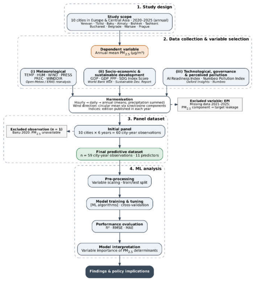
Figure 2.
Annual PM2.5 concentrations across the study cities, 2020–2025. Source: Authors’ calculations based on IQAir World Air Quality Reports, 2020–2025 [16,17,18,19,20,21].
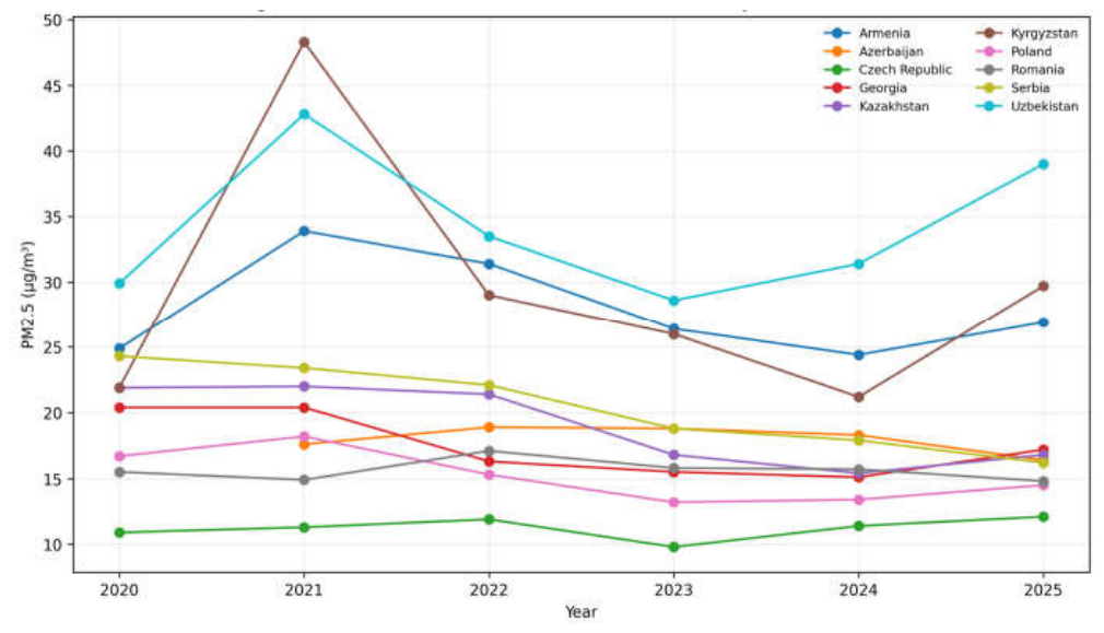
Figure 3.
Predictive performance of candidate machine learning models. Source: Authors’ calculations based on the study dataset.
Figure 3.
Predictive performance of candidate machine learning models. Source: Authors’ calculations based on the study dataset.
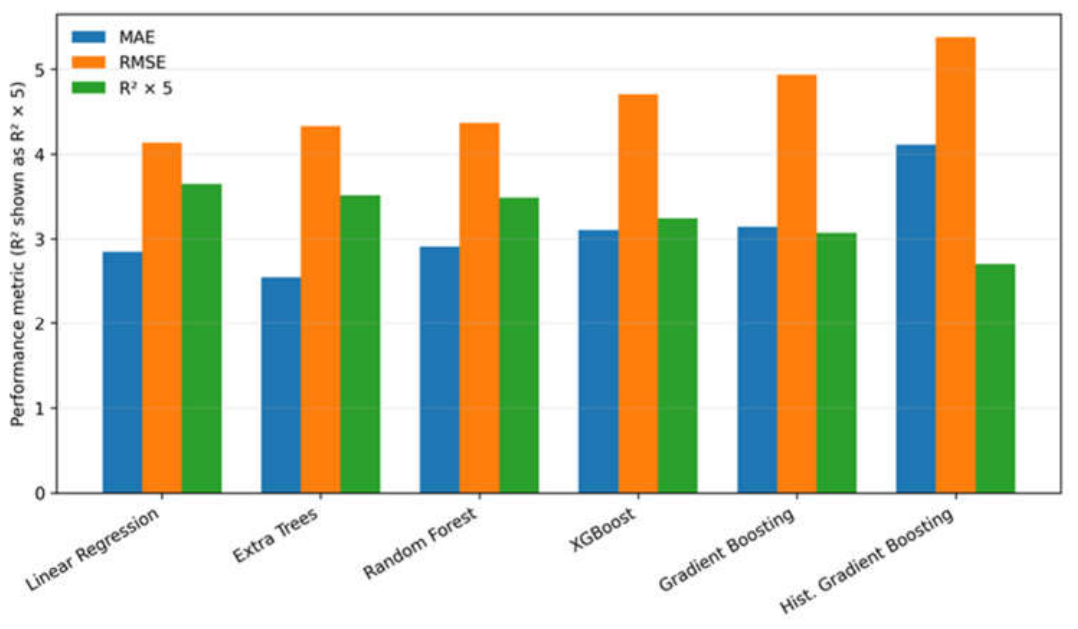
Figure 4.
Observed versus cross-validated predicted PM2.5 concentrations. Source: Authors’ calculations based on the study dataset.
Figure 4.
Observed versus cross-validated predicted PM2.5 concentrations. Source: Authors’ calculations based on the study dataset.
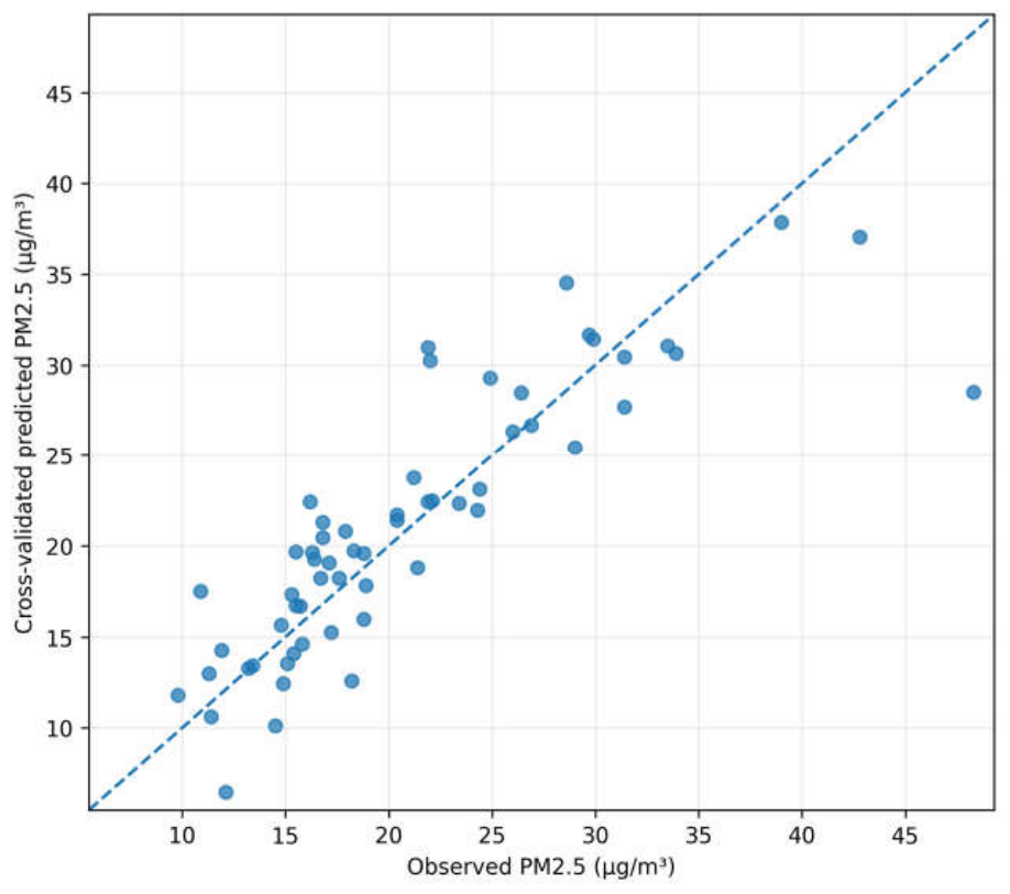
Figure 5.
Global predictor importance based on SHAP. Source: Authors’ calculations based on the selected machine learning model and study dataset.
Figure 5.
Global predictor importance based on SHAP. Source: Authors’ calculations based on the selected machine learning model and study dataset.
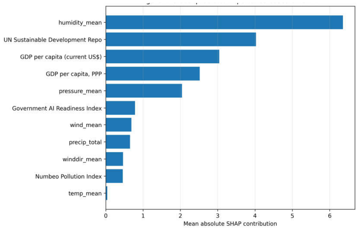
Figure 6.
Country-level comparative PM2.5 Risk Scores. Source: Authors’ calculations based on model-predicted PM2.5 concentrations.
Figure 6.
Country-level comparative PM2.5 Risk Scores. Source: Authors’ calculations based on model-predicted PM2.5 concentrations.
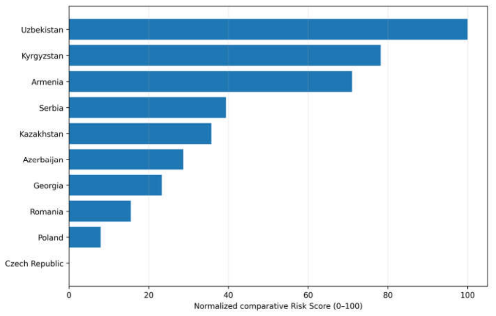

Table 1.
Predictive performance of candidate models Source: Authors’ calculations based on the study dataset.
Table 1.
Predictive performance of candidate models Source: Authors’ calculations based on the study dataset.
| Model | MAE | RMSE | R2 |
| Linear Regression | 2.850 | 4.134 | 0.729 |
| Extra Trees | 2.550 | 4.330 | 0.703 |
| Random Forest | 2.909 | 4.369 | 0.698 |
| XGBoost | 3.105 | 4.706 | 0.649 |
| Gradient Boosting | 3.141 | 4.934 | 0.614 |
| HistGradientBoosting | 4.110 | 5.380 | 0.541 |
Table 2.
Global SHAP-based importance of explanatory variables. Source: Authors’ calculations based on the selected Linear Regression model and the study dataset.
Table 2.
Global SHAP-based importance of explanatory variables. Source: Authors’ calculations based on the selected Linear Regression model and the study dataset.
| Predictor | Mean absolute SHAP | Standardized coefficient |
| Relative humidity | 6.358 | −6.970 |
| SDG Index Score | 4.026 | +4.623 |
| GDP per capita (current US$) | 3.042 | −3.745 |
| GDP per capita, PPP | 2.520 | −2.939 |
| Surface pressure | 2.042 | +2.283 |
| Government AI Readiness Index | 0.783 | +0.920 |
| Wind speed | 0.688 | −0.862 |
| Precipitation | 0.653 | −0.820 |
| Wind direction | 0.464 | +0.602 |
| Numbeo Pollution Index | 0.455 | +0.549 |
| Temperature | 0.041 | +0.049 |
Table 3.
Country-level comparative PM2.5 Risk Scores. Source: Authors’ calculations based on model-predicted PM2.5 concentrations.
Table 3.
Country-level comparative PM2.5 Risk Scores. Source: Authors’ calculations based on model-predicted PM2.5 concentrations.
| Country/City | Observed mean | Predicted mean | Risk Score | Category | |
| 1 | Uzbekistan (Tashkent) | 34.20 | 33.84 | 100.00 | Very High |
| 2 | Kyrgyzstan (Bishkek) | 29.35 | 29.13 | 78.20 | High |
| 3 | Armenia (Yerevan) | 27.98 | 27.58 | 71.03 | High |
| 4 | Serbia (Belgrade) | 20.45 | 20.74 | 39.37 | Low |
| 5 | Kazakhstan (Almaty) | 19.05 |
19.95 | 35.73 | Low |
| 6 | Azerbaijan (Baku) | 18.00 | 18.43 | 28.68 | Low |
| 7 | Georgia (Tbilisi) | 17.48 | 17.26 | 23.27 | Low |
| 8 | Romania (Bucharest) | 15.63 | 15.58 | 15.49 | Very Low |
| 9 | Poland (Warsaw) | 15.22 | 13.94 | 7.93 | Very Low |
| 10 | Czech Republic (Prague) | 11.23 | 12.23 | 0.00 | Very Low |
Disclaimer/Publisher’s Note: The statements, opinions and data contained in all publications are solely those of the individual author(s) and contributor(s) and not of MDPI and/or the editor(s). MDPI and/or the editor(s) disclaim responsibility for any injury to people or property resulting from any ideas, methods, instructions or products referred to in the content. |
© 2026 by the authors. Licensee MDPI, Basel, Switzerland. This article is an open access article distributed under the terms and conditions of the Creative Commons Attribution (CC BY) license (http://creativecommons.org/licenses/by/4.0/).
Copyright: This open access article is published under a Creative Commons CC BY 4.0 license, which permit the free download, distribution, and reuse, provided that the author and preprint are cited in any reuse.