
Submitted:
13 October 2026
Posted:
14 October 2026
You are already at the latest version
Abstract
Useful quantum-key supply from intermittent satellite contacts depends on finite-block security, authentication, relay inventories, and application demand, not optical transmittance alone. We simulate a trusted high-altitude-platform (HAP) relay between a ground station and a 500 km low-Earth-orbit satellite using three-intensity decoy-state BB84, finite-key estimation, authenticated key inventories, and a 200-pass service model. The comparator is the satellite-to-ground (S→G) downlink; a groundto-satellite uplink is not simulated, so the margins apply only to this downlink. With a 0.20 m HAP receive radius, the relay yields 13.175 Mbit/pass, 15.65% of the 84.185 Mbit/pass direct yield. With a 0.50 m HAP radius, the relay yield rises to 116.981 Mbit/pass, 38.77% above the 84.298 Mbit/pass direct yield. The unchanged direct-link estimates vary by under 0.2% from independent Monte Carlo sampling. The advantage remains 29.57% under a common contact window and 28.42% with equal elevation masks. Protocol tuning raises the 0.20 m relay yield by 36.74% without closing its gap to the direct link. For workloads derived from the 0.20 m relay supply, a 30 Mbit buffer produced no starved schedules for the 0.50 m relay in 10,000 simulations per demand. Receive-aperture collection is the main modeled condition for relay advantage under the stated assumptions.
Keywords:
quantum key distribution
; high-altitude platform
; trusted relay
; satellite quantum communication
; decoy-state BB84
; finite-key analysis
; key management
; service availability
1. Introduction
Quantum key distribution (QKD) allows two endpoints to establish shared secret material by combining quantum transmission with an authenticated classical channel. Decoy-state BB84 makes weak-coherent-pulse implementations more robust to photon-number-splitting attacks, while finite-key analysis accounts for the statistical uncertainty and security penalties that arise when only a limited number of detections is available [1,2]. These finite-resource effects are particularly important for satellite QKD: a low-Earth-orbit terminal is visible from a ground site for only a bounded interval, and diffraction, pointing, atmospheric loss, and background counts reduce the detection sample accumulated during that interval [3,4,5]. Consequently, a positive instantaneous or asymptotic rate does not by itself determine how much composably secure key a pass can deliver.
Satellite experiments have demonstrated that a trusted mobile node can establish separate keys with remote ground stations and combine them through an authenticated exclusive-or record [6]. A high-altitude platform (HAP) offers a different placement for such a trusted endpoint. Operating in the stratosphere can shorten one terrestrial optical path and place a receiving terminal above much of the dense lower atmosphere; feasibility studies have therefore examined HAP-to-ground QKD link budgets at approximately 20 km altitude [7]. A composable trusted-relay architecture placing the XOR combination at the HAP, together with a preliminary link-level feasibility case for satellite–HAP key sharing, was proposed by the present authors [8]. More recent aerial-network work has modeled balloon-to-ground, ground-to-balloon, and balloon-to-balloon channels and explored the resulting QKD network architectures [9]. These studies motivate HAP-assisted QKD, but none of them — including our own preceding proposal — established under which hardware configuration a relay is actually beneficial: the received aperture, pointing residual, background, contact window, and trust and resource costs remain decisive, and were not previously evaluated together in one accounting.
The architectural comparison must also extend beyond optical transmittance. In a trusted two-hop relay, each released end-to-end bit consumes one unused bit from each hop, and authenticated public communication consumes additional secret material. Post-processing delays when newly generated bits become usable, while application requests can be served only from key that has already reached the relevant inventory. An architectural study therefore needs to distinguish the secret key produced by each link, the authenticated end-to-end supply available after hop pairing, and the fraction of application demand served over a sequence of passes. Improving the first quantity does not guarantee the other two when the hop inventories or release times are unequal. Standards for QKD key delivery explicitly separate network key generation from application retrieval and identify key-management entities, key identifiers, and stored key pools [10]. This separation makes application availability a distinct question from whether either optical link produces a nonzero key.
This study asks the following scoped question: under the declared optical, finite-key, authentication, trust, and service assumptions, when does a trusted HAP relay deliver more usable key than a direct satellite–ground downlink, and how much application-buffer capacity is required for a fixed demand profile? The direct SG comparator is deliberately modeled as the favorable S→G downlink. It uses the same satellite-originating transmission direction as the SH relay hop, while retaining its own receiver, range, atmospheric path, elevation mask, and contact duration. A direct G→S uplink is outside the evaluated scope and is not inferred from the downlink results. Accordingly, all reported relay/SG performance margins in this study apply only to the modeled S→G downlink benchmark and should not be interpreted as performance relative to a direct uplink.
The paper makes the following contributions:
- It integrates a pass-dependent free-space channel surrogate with three-intensity decoy-state finite-key BB84, explicit authentication-resource debits, trusted-relay inventory pairing, post-processing timing, and application-key buffering. The contribution is this scoped system evaluation, extending the composable XOR-relay architecture of [8] with a full finite-key, authentication-accounted, and service-level numerical analysis; no new QKD security proof or relay protocol is claimed.
- It compares six controlled cases that separate HAP receive-aperture effects from contact-window and elevation-mask effects. Both a 0.20 m reference HAP receive radius and a 0.50 m matched radius are evaluated against the S→G downlink using full and common temporal supports. These controls isolate aperture, contact-window, and elevation-mask effects within the downlink comparison; they do not evaluate the propagation-direction effect associated with a direct G→S uplink.
- It connects weather-conditioned per-pass key production to a 200-pass service experiment with fixed workloads, finite buffers, authentication reserves, and no-backlog accounting. An equal-budget protocol search over the decoy intensities and basis probability (simulated annealing against grid and random-search baselines) shows that protocol tuning alone raises the 0.20 m relay yield by 36.74%, and one-factor sensitivity analyses identify which declared hardware and channel parameters most strongly affect the modeled relay supply.
The numerical results are conditional rather than universal. With the 0.20 m HAP radius, the full-contact relay produces 13.175 Mbit/pass, only 15.65% of the 84.185 Mbit/pass SG yield. With the 0.50 m matched radius, the relay produces 116.981 Mbit/pass and exceeds its 84.298 Mbit/pass SG comparator by 38.77% under the modeled full contacts. The common-window and equal-mask controls preserve a smaller advantage. These results identify aperture collection as the principal modeled condition separating the two outcomes; they do not establish hardware feasibility or performance under unmodeled cloud blockage, calibrated turbulence, or a direct uplink.
The remainder of the article is organized as follows. Section 2 positions the study relative to satellite and aerial-platform QKD, atmospheric channel models, finite-key analyses, and key management. Section 3, Section 4, Section 5 and Section 6 define the architecture, implemented channel and detection model, finite-key and authentication accounting, relay release, service process, and protocol search. Section 7 reports the configuration, numerical checks, key yields, availability, optimization, and sensitivity results. Section 8 discusses their interpretation and limitations, and Section 9 concludes the study.
2. Related Work
2.1. Satellite QKD and Trusted Relaying
Low-Earth-orbit (LEO) satellite QKD has been demonstrated experimentally, including intercontinental key exchange in which a satellite acts as a trusted node that establishes separate keys with two distant ground stations and combines them through a public exclusive-or record [6], and the state of satellite QKD technology, missions, and open engineering challenges has been reviewed in [11]. Link-budget and mission-design studies of this kind established the diffraction-, pointing-, and atmosphere-limited character of a single LEO pass and the resulting design trade-offs among transmitter divergence, receiver aperture, and orbit selection [3]. The composable exclusive-or relay used in this paper follows the same trusted-node principle, applied instead to a stratospheric platform rather than to a second satellite pass, as we first proposed in [8]; the present paper supplies the finite-key, authentication, and service-level analysis that proposal did not include.
2.2. High-Altitude and Balloon Platforms
A high-altitude platform positioned near 20 km places a receiving terminal above much of the dense lower atmosphere while remaining far closer to the ground than any satellite orbit. Feasibility analyses of HAP-to-ground QKD have quantified the resulting link-budget advantage for that geometry and identified the residual pointing and background requirements it still imposes on the airborne terminal [7]. More recent work has extended this aerial-node concept to high-altitude balloons, modeling balloon-to-ground, ground-to-balloon, and balloon-to-balloon channels together with candidate QKD network architectures built from them [9]. These studies, together with our own earlier composable-relay proposal [8], motivate HAP- and balloon-assisted QKD as a placement strategy, but none of them evaluates whether a specific relay configuration actually outperforms a direct downlink once receiver aperture, authentication cost, and two-hop inventory pairing are all accounted for together, which is the gap this paper addresses.
2.3. Free-Space Channel Models
Atmospheric transmittance for terrestrial and slant free-space optical links is commonly modeled through a visibility-dependent extinction coefficient with a wavelength-dependent size-distribution exponent [12]; fog, rain, and snow attenuation measured on hybrid free-space optical/radio-frequency (FSO/RF) links shows that low-visibility weather, particularly fog, is a principal limitation of the optical path [13], consistent with current ITU-R propagation guidance [14]; we have previously used the same visibility-conditioned extinction approach to evaluate an FSO link under varying atmospheric visibility in a terrestrial high-speed-train scenario [15], and the present paper adopts the same discrete-visibility-category treatment for the satellite and HAP links. Turbulence-induced fading of a free-space quantum channel has been modeled in more physical detail through Rayleigh-distributed beam-centroid displacement combined with atmospheric structure parameters [16], a law-of-total-probability treatment of the resulting transmittance distribution [17], and direct numerical propagation simulation of the atmospheric channel [18]. Fundamental point-to-point capacity bounds for a lossy bosonic channel, used here only as an implementation diagnostic rather than as a claimed achievability result, were established in [19] (the Pirandola–Laurenza–Ottaviani–Banchi, PLOB, bound), and satellite-specific fundamental bounds encompassing both uplink and downlink configurations were derived in [20]. The present paper uses a declared, fixed-width Gaussian centroid-displacement surrogate rather than any of these more complete propagation models, trading physical fidelity for a channel that is exactly integrable and therefore auditable end to end; Section 4.2 states this scope explicitly.
2.4. Finite-Key Satellite Performance
Because a satellite pass supplies only a finite detection sample, an asymptotic key rate can substantially overstate the secret key a single contact can certify. This has been quantified directly for representative LEO passes [4], extended to a systematic finite-resource performance analysis across several proposed small-satellite QKD missions [5], and further developed into a practical-constraint performance model that incorporates engineering limitations such as bounded in-orbit parameter tunability and finite random-number generation and storage rates [21]. The three-intensity decoy-state protocol and its associated finite-key security bounds, which this paper adopts for every simulated link [1,2], originate in the same finite-block regime that these satellite-specific studies analyze. Unlike [4,5,21], which characterize single-link satellite-to-ground performance, this paper applies the same finite-key discipline to a two-hop trusted relay, where the accounting must additionally track authentication debits and inventory pairing across both hops before an end-to-end key length is defined.
2.5. Trust and Application-Key Availability
Trusted relays and untrusted measurement nodes represent different security architectures. In measurement-device-independent (MDI) QKD, an untrusted measurement station does not expose detector side channels [22]; MDI-QKD is not the protocol evaluated here. The HAP is instead an endpoint of both QKD sessions, learns both hop keys, and must remain trusted. service boundary, the European Telecommunications Standards Institute (ETSI) specification GS QKD 014 defines a REST-based application programming interface (API) through which key-management entities deliver identified blocks of key material to applications; it assumes secure operation of trusted nodes and leaves the internal generation and relaying of key material outside its scope [10]. This paper does not implement that API. It models the preceding resource process: generation, authentication reservation, one-time hop pairing, delayed release, bounded storage, and request service. The resulting availability metric therefore complements physical and finite-key link analyses without being interpreted as an optical-channel availability measurement. The one-time-pad exclusive-or combination used to publish the relay record is information-theoretically hiding for independent uniform operands under the classical secrecy argument of [23], provided a consumed mask is never reused, as enforced by the provenance check in Section 5.3. Authentication of every classical message in this accounting is represented through the universal-hashing construction of [24], and the composable security statement combining the finite-key, authentication, and relay parameters follows the general composability framework of [25]. The protocol-search procedure, defined in Section 6.3 and evaluated in Section 7.7, uses simulated annealing [26] together with grid and random-search baselines at equal evaluation budget, following standard practice for comparing a stochastic search against transparent baselines rather than claiming global optimality.
Taken together, the literature provides mature components for satellite link analysis, aerial-platform feasibility, finite-key estimation, trusted relaying, and application key delivery. The contribution here is to place selected components in one reproducible, explicitly bounded simulation and to expose when a favorable atmospheric location is outweighed by aperture collection or by two-hop inventory constraints. The conclusions remain tied to the modeled parameters and trust assumptions.
3. System, Protocol, and Trust Model
3.1. Architecture and Common Geometry
We consider a ground station G, a trusted high-altitude platform H, and a low-Earth-orbit satellite S. The reference HAP altitude is 20 km; satellite altitudes of 500–1200 km are scenario parameters, not inferred operating optima. The HAP reference is motivated by [7]. Both the assisted and direct architectures use the same satellite trajectory and ground location. The baseline quantum transmissions are G→H (GH uplink), S→H (SH downlink), and S→G (SG reference downlink). Thus, the HAP has two separate receiving terminals and the satellite transmitter can be matched between the SH and SG comparisons. Reversing the direct SG link to G→S requires recomputing its direction-specific propagation and receiver model; therefore, the simulated S→G downlink results are not reused as estimates of direct-uplink performance, and no G→S key yield is reported in this study. Figure 1(a) summarizes these nodes and link directions. The direct SG downlink is evaluated as a separate comparator scenario, not as a pulse stream shared simultaneously with SH, and all reported numerical cases use the 500 km satellite and 20 km HAP shown there.
The satellite follows a circular orbit arranged as an overhead pass of the ground station at latitude and longitude with inclination i: the initial argument of latitude is and the right ascension of the ascending node is , while the ground station and HAP rotate with the Earth.
Let be the Earth-centered position of node , expressed in one common coordinate frame. For nodes , define
For propagation from transmitter a to receiver b, the altitude along the ray is
Ground elevation masks, HAP field of regard, Earth occultation, and tracking acquisition define each usable contact interval . The HAP is fixed relative to the ground over one pass; its horizontal offset is specified as well as its altitude. Earth rotation must be included when positions are transformed from an orbital frame. All link calculations use Eqs. (1)–(2).
Comparisons report both each architecture’s full usable contact and a common contact window. Matching geometry does not match resources: the assisted architecture adds two optical terminals, a trusted site, and a second QKD session. Apertures, detector characteristics, pulse budgets, authentication budgets, and initial key inventories are therefore disclosed for every comparison. A HAP does not remove cloud blockage on the GH hop; adverse weather remains part of its availability model [3,7].
3.2. Trust, Authentication, and Relay Operation
The security claim concerns an external adversary controlling both quantum channels and observing or modifying public traffic, subject to authenticated communication and the characterized-device assumptions below. The HAP is an endpoint of both QKD sessions and knows both link keys. Consequently, an honest-but-curious HAP knows the relayed key, and a malicious or compromised HAP is outside the single-relay secrecy guarantee. This is the trusted-relay setting used in satellite key distribution [6]; it differs from MDI-QKD, whose measurement node need not be trusted [22].
Classical transcripts, key identifiers, sequence numbers, and relay messages are authenticated with a specified universal-hashing construction [24]. Each adjacent node pair starts with a secret authentication reserve. Tag-mask consumption, hash-key refresh or recycling, and rejected-message costs follow that construction; tag length alone is not the total authentication cost. Authentication keys and application keys use disjoint bit ranges.
Let be the unused link-key bits remaining after the reserves defined in Section 5.3 have been allocated. For one relay operation, the HAP selects disjoint, unused strings and of length
and transmits
G reconstructs the SH string, while S already holds it. Both endpoints verify the relay record before releasing the key; Figure 1(b) traces this sequence from the two hop inventories to the application buffers. The public XOR reveals no individual operand for ideal independent uniform keys [23]. Both selected link-key segments are retired from their link inventories; the SH segment is transferred to the end-to-end inventory. Previously unused surplus bits may be buffered and used once later. Reusing a consumed GH mask would expose
3.3. Per-Link Protocol and Block Definition
Each link runs polarization-encoded, phase-randomized, three-intensity decoy-state BB84 [1,2,27]. The transmitter chooses with
Transmitter and receiver independently choose the key basis X with probability and the test basis Z with probability [28]. Matching-basis probabilities are therefore and . All intensities contribute to the X-basis raw key, as in [2]. Parameters may differ between links. The reference wavelength is 1550 nm. The satellite source used in the SH and SG scenarios operates at 500 MHz, a repetition rate also used in the HAP QKD feasibility analysis of [7]; the 10 MHz GH source rate is an assumed study input. A pulse clock is not a detector count rate.
For bit a and basis b, the source state is
Conditioned on the photon number , encoding and other emitted degrees of freedom are assumed independent of the intensity label. Bits and settings are generated with private randomness; single-photon basis states and receiver responses satisfy the adopted security theorem. An active two-detector receiver assigns a random bit to double clicks. Accepted detections must not introduce an unmodeled basis-dependent efficiency or setting-dependent postselection.
Each block has a predetermined transmitted-pulse budget and a scheduled contact window. Settings and block boundaries are fixed before quantum transmission; basis information is disclosed after collection. Finite contact windows motivate pass-level evaluation [4]. A predeclared final, shortened contact block is processed if it passes the finite-key tests; otherwise, it is discarded. Thus, is an observed detection count, not an independently chosen deterministic input. This fixed-window baseline avoids an unspecified rule for repeatedly testing and stopping on favorable statistics. Parameters are optimized offline; adaptation within a block or data-selected time filtering requires a separate analysis. In the numerical evaluation of Section 7, each usable contact is processed as exactly one such block.
4. Channel and Detection Model
4.1. Diffraction and Atmospheric Extinction
For a Gaussian beam launched at its waist, denotes the intensity radius and its beam-quality factor. The diffraction-broadened beam radius , divergence angle , and centered aperture collection fraction are
where is the receiver-aperture radius.
Finite launch apertures and beam truncation must be consistent with and . Divergence is not varied independently of these quantities without an explicit optical model. No additional loss is applied [29].
Let be a power-extinction coefficient in . With s in meters,
For visibility V in km defined at a 2% contrast threshold, the near-ground aerosol approximation is
The Kim exponent is
The model follows [12,14]. The coefficient in Eq. (7) is an extinction coefficient in natural-logarithm units (); its decibel counterpart dB/km follows from the conversion in Eq. (6). Visibility reported using a different contrast threshold must first be converted consistently.
The altitude profile separates molecular and aerosol terms, for example,
where is the molecular extinction coefficient and is a specified dimensionless aerosol-layer profile with ground value one. The factor converts from to . The chosen layer depth or decay scale is a model input. A separately modeled cloud-occultation state sets the affected quantum link to unavailable; the visibility formula is not a universal cloud or precipitation model. Aerosol extinction is not added again if already contained in a measured or radiative-transfer extinction profile.
Writing
where and denote the transmitter and receiver optical throughputs, respectively, the instantaneous channel and signal-detection efficiencies are
Here, is the instantaneous aperture-collection fraction, is the detector efficiency, and is the fraction of the photon arrival-time distribution accepted by the gate. Detector efficiency and temporal acceptance are excluded from reported optical channel transmittance.
4.2. Turbulence and Collected-Power Statistics
The reference Hufnagel–Valley (HV) profile for the refractive-index structure parameter is
where h is the altitude in meters, v is the wind-speed parameter, and is expressed in [30]. The HV-5/7 reference uses m/s and , where A is the coefficient of the near-ground turbulence term. The exact profile value at is therefore rather than A alone. The altitude definition is consistent with Eq. (2).
For link j, let denote the transmitter-to-receiver propagation distance and let s denote the position along that path, with . The corresponding plane-wave and spherical-wave weak-fluctuation diagnostics are
where is the altitude along link j and is the optical wavenumber. The plane-wave and spherical-wave expressions are used only as diagnostics for their respective illumination limits and are not interchangeable Gaussian-beam propagation models. A diagnostic value below 0.3 is used only as a conservative weak-regime screen; it does not validate an aperture-transmittance model.
The aperture-collected power fraction for link j is defined from the normalized receiver-plane irradiance as
where is the two-dimensional position in the receiver plane and is the receiver-aperture radius. The normalization makes the fraction of the incident optical power collected by the receiver aperture.
For the implemented surrogate model, the beam-centroid displacement is modeled as a Gaussian random displacement with per-axis variance , while the short-term beam radius is fixed. Defining , the collected fraction for a given centroid displacement is
where is the first-order Marcum Q-function. Equation (13) gives the exact circular-aperture integral for this fixed-width Gaussian beam profile; it is not an exact description of an arbitrary turbulent beam. No calibrated elliptic-beam or scintillation model, and no extra log-normal or Gamma–Gamma multiplier, is applied to this surrogate; a validated alternative would require calibration data that and a Rytov value alone do not supply [16,18].
4.3. Residual Pointing and Temporal Dependence
For one angular pointing axis, let f denote temporal frequency, the open-loop gain of the tracking loop, the angular-disturbance power spectral density (PSD), and the equivalent angular sensor-noise PSD. For uncorrelated disturbance and sensor-noise inputs, the residual angular-error PSD is
Here, is the residual pointing-error PSD after tracking correction, and is the corresponding per-axis angular-error variance. The one-sided PSDs have units , so has units of radians. Bandwidth alone does not determine ; loop gain, delay, sensor filtering, stability, and finite noise bandwidth must also be specified [31,32]. A tracking-bandwidth () sweep of 50–700 Hz used in Section 7.8 is a design study, not a measured HAP capability. Satellite pointing demonstrations provide context, not transferable HAP disturbance spectra [33,34].
In the numerical study, the loop is a modeled first-order tracking response with , so that and , with a baseline closed-loop bandwidth Hz. The assumed spectra are /Hz and /Hz. The integral in Eq. (14) is evaluated over 0.01–2000 Hz with 400 logarithmically spaced nodes and trapezoidal quadrature, giving a baseline per-axis residual rad. These spectra are study assumptions, not a measured HAP controller.
For transmitter angular error, the received pointing, acquisition, and tracking (PAT) displacement is . For link j, let denote the per-axis variance of the Gaussian beam-centroid displacement used in the surrogate model above. Assuming that residual atmospheric centroid wander and residual pointing error are independent, this variance is
where is the per-axis residual atmospheric centroid-wander standard deviation, is the per-axis residual angular pointing-error standard deviation defined from Eq. (14), and converts the angular pointing error to a receiver-plane displacement.
In the baseline model, for all links, so the centroid-displacement variance is due entirely to residual pointing. Averaging Eq. (13) over the resulting Rayleigh-distributed centroid offset gives the mean aperture-collection fraction ; its integral form and closed-form expression are given in Appendix A, and it is the quantity plotted in Figure 3(c) and Figure 4. A marginal probability distribution of transmittance (PDT) does not specify fade; independent samples are used only for bins explicitly assumed decorrelated, and the implementation does not simulate correlated within-pass fading trajectories.
4.4. Receiver Counts and Block Statistics
For an active receiver with two symmetric detectors, let denote the dark-count rate of each detector and let denote the spectral radiance incident at the receiver entrance aperture, in . A single baseline radiance is assumed for all links, with sensitivity to this value examined in Section 7.8, rather than using a calibrated day/night radiance model.
The aggregate mean background-photon count admitted during one detection gate is
where is the receiver throughput for background light, is the detector efficiency, is the receiver-aperture area, is the receiver field-of-view solid angle (sr), is the optical filter bandwidth (nm), and is the detection-gate duration. Here, is Planck’s constant, c is the speed of light, and is the photon energy at wavelength . The quantity is therefore the noise-click probability of one detector during one gate. The factor accounts for the equal sharing of unpolarized background light between the two detectors.
For the circular receiver aperture used here, . Following [3,35], the corresponding aggregate vacuum yield, i.e., the probability that at least one of the two detectors clicks in the absence of signal photons, is
Conditioned on a matched basis and an encoded bit, let denote the intrinsic optical-error probability for link j. The symmetric error model directs fractions and of the signal to the correct and wrong detectors, respectively. For compactness, the link index j is suppressed in the following detector-response expressions, so that and . Defining
where x is the mean detected signal-photon number for intensity setting k, the correct- and wrong-detector click probabilities are
Here, and are the click probabilities of the correct and wrong detectors, respectively; is the total detection probability (gain), is the error gain, and is the corresponding quantum bit error rate for basis b and intensity setting k. The term assigns a random bit to a double-click event, consistent with the receiver rule specified in Section 3.3. This conditional Poisson model therefore treats double clicks explicitly.
This is a performance model; the security estimator uses the actual accepted counts without assuming that Eve follows this channel law. The analytic baseline is valid in the low-occupancy regime with negligible afterpulsing, requiring
for each detector, where is the transmitted-pulse repetition rate, is the detector click rate, and is the detector dead time. Section 7.1 reports the maximum realized value of the click-rate–dead-time product across the numerical study. With fixed settings, the planning means are
Average gains and error gains are accumulated before forming the quantum bit error rate (QBER); in general . Expected-count optimization (used for the planning objective of Section 7.7 and the diagnostic of Section 7.4) is a planning approximation; finite-block distributions require integer count realizations, which are what the main numerical results of Section 7 use.
5. Finite-Key Security and Trusted-Relay Composition
5.1. Count Bounds and Phase-Error Estimation
We adopt the three-intensity finite-key estimator of [2,36]. For clarity, the link index is omitted. Let and denote the observed detection and error counts, respectively, for basis and intensity k, with
where is the overall probability of emitting n photons. With the statistical failure-budget share ,
Negative lower bounds are clipped at zero. For the vacuum-plus-weak setting,
where ; and are lower bounds on the vacuum and single-photon detections, and is an upper bound on the single-photon Z-basis errors. Inconsistent or empty confidence regions cause an abort. Setting ,
Here, is the upper bound on the single-photon X-basis phase-error rate. We use the convention of [2], retaining the full secrecy parameter and the factor 21. The block is aborted if , , , the logarithm is outside its domain, or . Zero observed errors do not imply zero phase error. A tighter Chernoff estimator [37] is not used here.
5.2. Per-Block Key Length and Security Meaning
For reconciled X-basis strings, the extracted key length is
where is the binary entropy function, is the error-correction leakage, and . With the link index omitted, planning calculations use , , for specified [38,39].
Correctness and secrecy are specified by and , where and are the accepted endpoint keys, is the abort probability, and and denote the actual and ideal key–adversary states, respectively. These are composable distinguishing guarantees, not per-bit compromise probabilities [25].
For a stationary, infinite-data reference using all intensities, the corresponding rate in bits per emitted pulse is
Here, and are the asymptotic lower bounds on the vacuum and single-photon yields, respectively, and is the corresponding upper single-photon phase-error rate. Equation (23) suppresses statistical deviations and additive finite-security penalties and is used only as the convergence reference in Section 7.4.
5.3. Authentication Accounting and Composition
Allocate disjoint QKD outputs to authentication replenishment and relay authentication on each hop. Let denote their total allocation, with . The newly available relay inventory is
This is net-growth accounting. An aborted session can still consume pre-existing authentication bits; a separate reserve ledger tracks these debits, and operation stops when authentication cannot be funded. No application key is relayed until the required reserves are available. The implemented profile uses 128-bit tags and as an idealized authentication abstraction; Section 8.3 states this limitation.
For one block pair and relay operation, a sufficient external-adversary security allocation is
Here, and are the authentication failure parameters for QKD-link communication and the relay operation, respectively, and is the resulting end-to-end security parameter. Equation (25) follows from contractivity under classical processing and the triangle inequality [25]. Over multiple passes, the security parameters of all used QKD blocks and authentication operations are summed once toward the system-lifetime target.
6. Key Release, Availability, and Optimization
6.1. Block Completion and Release Latency
For a fixed emitted-pulse block on link j, let and denote the block start and acquisition-end times, respectively. For a sequential post-processing schedule, define
Here, , , , , , , and are the communication, sifting, parameter-estimation, error-correction, error-verification, privacy-amplification, and authentication times, respectively.
For relay operation r, let denote the request time, with and the ready times of the associated GH and SH blocks. For parallel link processing,
The relay duration includes transmitting the -bit XOR record, identifiers, and authentication, where is the relayed key length for operation r; is the corresponding request-to-release latency. Stored keys can satisfy a request without waiting for new quantum transmission. The numerical post-processing and relay-serialization parameters are listed in Table A1 (Appendix B).
6.2. Link Inventories and End-to-End Service
Let be the unused authenticated link inventory before update q, and the newly ready net link bits. With link capacity ,
Here, is the inventory after adding the newly ready bits and before relay pairing, and is the amount paired across the link inventories at update q.
For end-to-end capacity , let be the available application-key buffer before demand , and let be the newly released end-to-end key arriving after that demand. Under a demand-before-arrival convention,
Here, is the served demand and the unmet demand; overflow is recorded, and queued-demand service, if used instead, requires its own queue state [10,40].
Let denote the pass to which relay operation r is assigned and the deadline of pass p. Finite-block yield is attributed to the designated pass even if post-processing finishes later:
Thus, is the total generated relay key attributed to pass p, whereas counts only key released by its deadline.
For a fixed observation horizon , define
Here, is the probability of no starvation over the full horizon, whereas is the fraction of demand-bearing updates served without starvation. Neither quantity is identical to optical-transmittance outage. Confidence intervals are reported across independent simulated schedules; zero observed starvation events do not establish zero risk, as discussed quantitatively in Section 7.6.
6.3. Constrained Design and Numerical Evaluation
For each link, the design vector in principle includes
and hardware may instead be fixed by a terminal design. Let collect the design variables across the links and denote their feasible design set. For stochastic channel scenarios, the primary design problem is
Zero-key blocks and unsuccessful passes remain in this expectation. Given a selected design and declared initialization policy, buffer sizing is
Here, is the maximum candidate buffer capacity and is the required horizon availability. An empty feasible set is reported as infeasible. The pulse-budget variable is searched on a discrete grid; continuous variables are optimized with simulated annealing or another stated derivative-free method [26]. Candidates share channel realizations during optimization, after which the selected design is tested on independent realizations to expose selection bias. Coarse-grid and equal-budget random-search baselines separate joint-design gains from search effort; no global optimality or convexity is claimed. Section 7.7 restricts the evaluated design vector to with hardware, processing, and service settings fixed at the values of Table 1.
Before producing results, the implementation checks deterministic limits, extinction units, aperture bounds, PDT normalization and moments, count bookkeeping, finite-key abort rules, authentication reserves, and conservation of bits through both inventories, as summarized in Section 7.1 and listed individually in Table A2 (Appendix C).
7. Simulation Setup and Numerical Results
This section evaluates the trusted-relay architecture under the fixed numerical configuration summarized in Table 1. The comparisons use the same ground location and satellite trajectory while varying the HAP receive radius, HAP elevation mask, and temporal support of the calculation. Unless stated otherwise, results use a 500 km satellite altitude, a 20 km HAP vertically aligned with the ground station, and the full usable contact interval of each link. Confidence intervals quantify integer-count sampling uncertainty within the model; they do not include uncertainty in the assumed hardware or atmospheric parameters.
7.1. Configuration, Comparison Cases, and Numerical Checks
The scenario geometry consists of study assumptions rather than a specific mission. The ground station is located at N, E. The satellite follows a circular 500 km orbit with an inclination of , typical of a sun-synchronous low-Earth orbit at this altitude. The ground elevation mask is , which excludes low-elevation paths with long atmospheric propagation; the reference HAP mask is because the stratospheric terminal lies above most of the dense atmosphere, and the equal-mask cases of Table 2 test the effect of this choice. Optical transmission is modeled at 1550 nm. The GH source operates at 10 MHz, and the satellite source used in the separate SH and SG scenarios operates at 500 MHz. Each usable contact is processed as one predetermined finite-key block (Section 3.3). For every combination of case, link, and visibility, 64 integer-count realizations are generated after averaging the gain and error gain over the Gaussian centroid-displacement distribution (Eq. (18)). Counts are drawn separately in each integration bin i containing pulses. The six accepted detection classes , , , , , and a residual no-detection or basis-mismatch category are drawn jointly from a multinomial distribution with class probabilities , implemented as sequential conditional binomial draws; the six detection counts are therefore not independent. Conditional on each detection count , the error count is binomial with parameters and , where and are the radially averaged gain and error gain of Eq. (18). Bin counts are summed over the contact before finite-key estimation. A zero gain produces zero accepted detections and zero errors. Binomial variates use inversion when and BTRD rejection sampling otherwise.
Table 2 defines the six evaluated cases. A full-contact case uses every link’s own valid interval. A common-window case restricts GH, SH, and SG to their temporal intersection so that the compared keys share the same temporal support. The equal-mask cases set the HAP mask to to separate the effect of the HAP’s lower reference mask from that of its receiver aperture. These controls do not make the two architectures resource-equivalent: the assisted architecture still uses a trusted platform, two QKD links, and additional optical and classical equipment.
For the service experiment, one modeled contact recurs every s, the circular-orbit period at 500 km with the Earth constants of Table 1. The local pass origin is the start of the s geometry span, 450 s before the overhead reference epoch. A first-order Markov chain selects the pass visibility with , where are the stationary probabilities of Table 1; the chain starts from a stationary draw and undergoes 100 initialization transitions. GH, SH, and SG share the visibility state of a pass. Conditional on that state, each link independently selects one of its 64 stored integer-count realizations uniformly with replacement. The four requests of a pass occur at , , after the pass origin (approximately 1417.036, 2834.072, 4251.108, and 5668.144 s). Link, relay, and application payload inventories start empty after the weather initialization; each hop inventory has a capacity of bits. The end-to-end demand assigned to one pass is 50%, 90%, 105%, or 130% of the weather-weighted reference/full relay supply and is divided equally among four requests. The same absolute workloads are then applied to every hardware case. Unmet demand is partially served and discarded rather than queued, and generated keys do not expire within the 200-pass horizon.
The full numerical run passed all 40 mandatory numerical and accounting checks (Table A2). These checks are not prescribed by a standard; they were designed for this study to verify internal consistency of the implementation against analytic identities, conservation laws, and declared tolerances. They included probability and count consistency, contact-boundary and Earth-occultation checks, aperture-integral identities, finite-key abort behavior, authentication-reserve nonnegativity, one-time XOR provenance, inventory conservation, PLOB comparisons, time-step refinement, and reproducibility. The maximum detector click-rate–dead-time product was 0.0125, below the imposed 0.05 limit. Reducing the integration step from 5 to 2.5 s changed the reported quantities by at most in relative terms. A repeated full numerical study reproduced 801,266 numerical values byte-for-byte. These checks support computational consistency; they do not constitute independent physical calibration of the channel model.
7.2. Contact Geometry
Figure 2 shows the reference contact geometry. GH spans the complete s simulation interval, giving a duration of 900 s and emitted pulses. This duration is the selected simulation span for the vertically aligned ground–HAP pair, rather than a derived finite visibility interval. With the HAP mask, SH is available from to s, or 425.524 s, containing approximately emitted pulses. The ground mask limits SG to to s, or 292.665 s, containing approximately pulses.
The longer SH interval therefore arises partly from the lower reference HAP mask. The common-window cases remove that temporal advantage by restricting every link to the same overlap, whereas the equal-mask cases set both satellite-facing receivers to . These controls are used below to distinguish contact-time effects from aperture-collection effects.
7.3. Optical Collection and Per-Link Finite-Key Yield
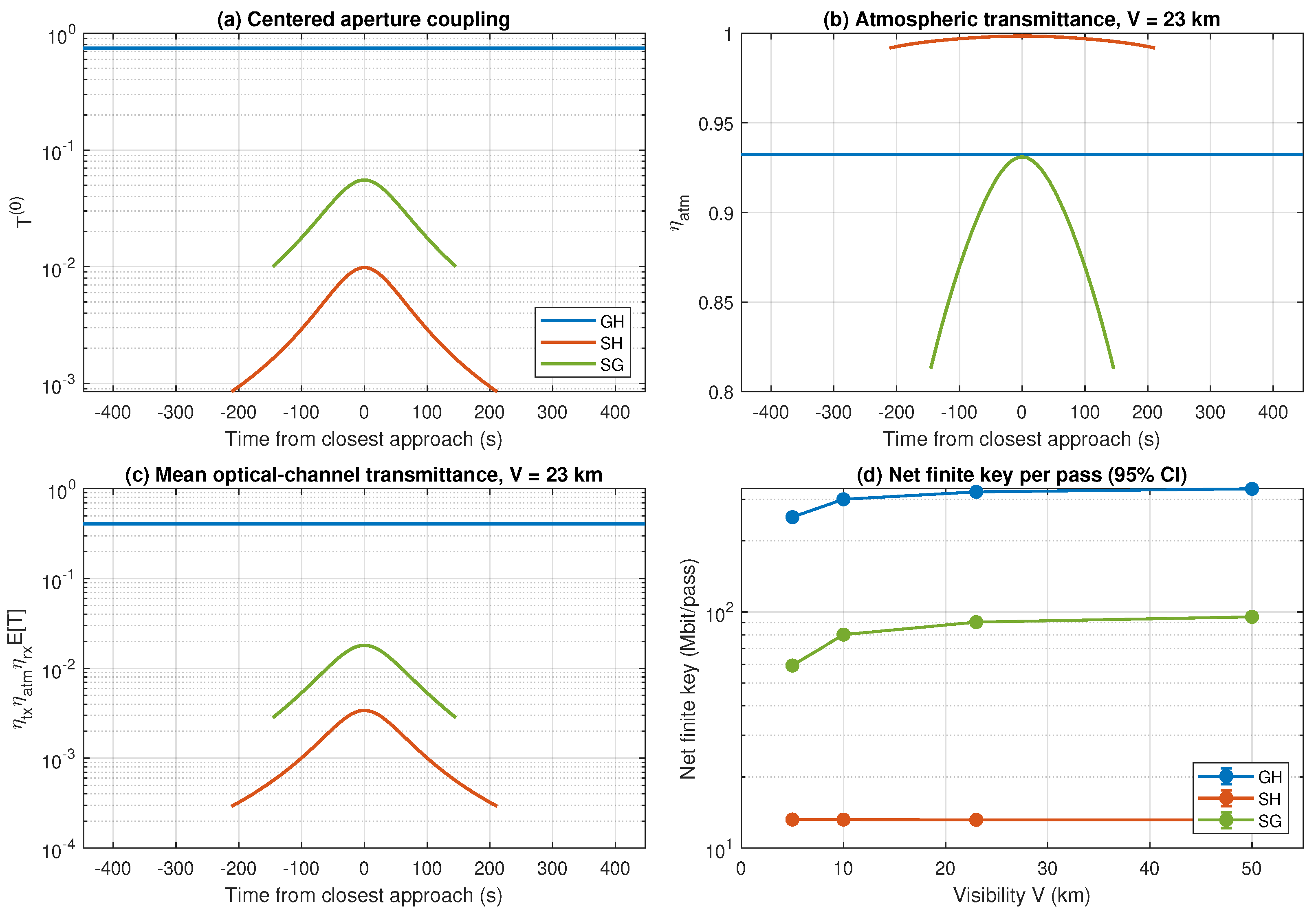
Figure 3 separates the principal terms in the reference link budget. The centered GH collection is high because of its 20 km range, whereas the much longer SH and SG paths are dominated by diffraction, aperture size, and residual pointing displacement. At km, SH experiences little extinction because most of the ray lies above the lower atmospheric layer, but its 0.20 m HAP receiver collects only a small fraction of the incident beam. SG crosses more of the lower atmosphere, although its 0.50 m ground receiver provides greater aperture collection than the reference HAP receiver. Consequently, low atmospheric extinction alone does not guarantee a large finite key.
Figure 3.
Reference-hardware link budget and net finite key. (a) Centered Gaussian-aperture collection , Eq. (5). (b) Atmospheric transmittance at km, Eq. (6). (c) Mean pre-detection optical-channel transmittance ; detector efficiency and gate acceptance are excluded. (d) Net finite key per pass versus visibility; error bars are 95% Monte Carlo confidence-interval half-widths over 64 integer-count realizations (at most 0.5% of the mean) and are smaller than the markers.
Figure 3.
Reference-hardware link budget and net finite key. (a) Centered Gaussian-aperture collection , Eq. (5). (b) Atmospheric transmittance at km, Eq. (6). (c) Mean pre-detection optical-channel transmittance ; detector efficiency and gate acceptance are excluded. (d) Net finite key per pass versus visibility; error bars are 95% Monte Carlo confidence-interval half-widths over 64 integer-count realizations (at most 0.5% of the mean) and are smaller than the markers.
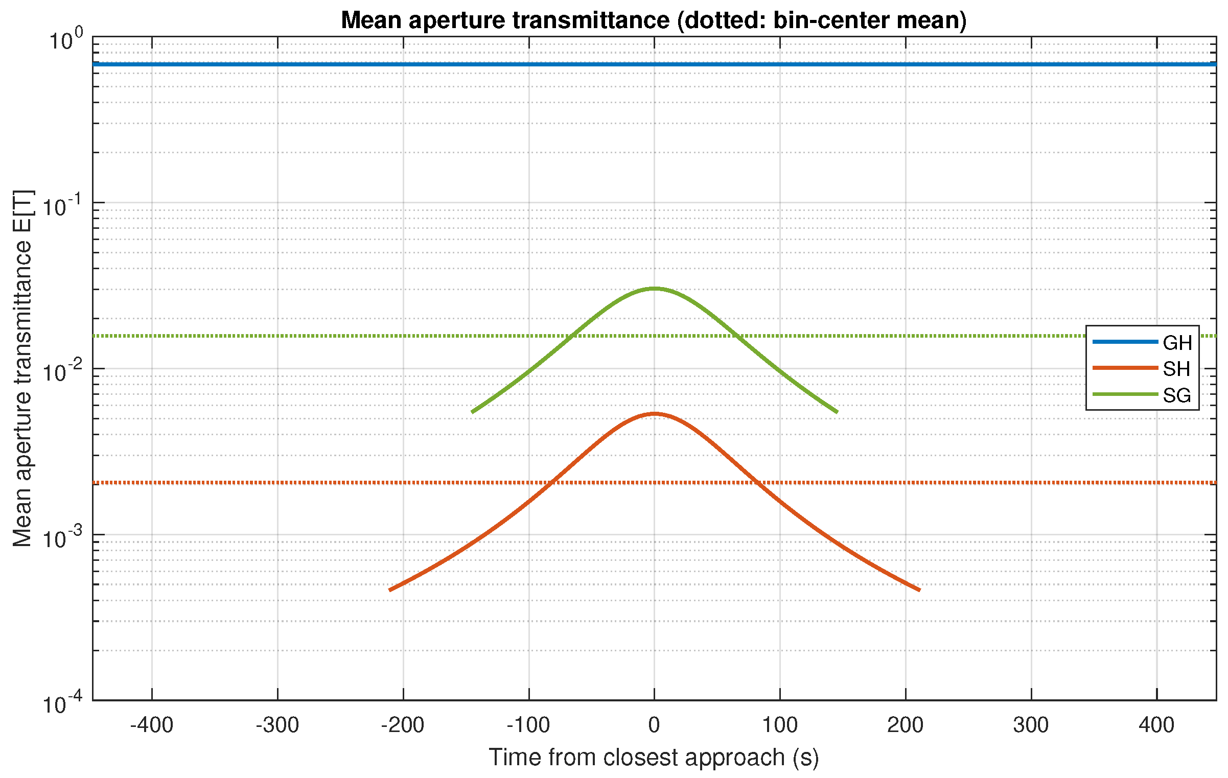
The mean aperture-transmittance trajectories in Figure 4 reinforce this interpretation. The reference SH collection remains below that of SG throughout their contacts, while GH has a much larger and nearly constant value. The fixed-width Gaussian centroid-wander surrogate of Section 4.2 produces these means; they should not be interpreted as measured turbulence distributions. When the receiver and detection models are applied, SH becomes the limiting relay hop in the reference configuration, as shown by the net finite-key results in Figure 3(d).
Figure 4.
Mean aperture transmittance of the fixed-width Gaussian centroid-displacement surrogate, Eq. (A1), over each reference contact. Dotted lines indicate the arithmetic mean over integration-bin centers for each link. Atmospheric extinction, transmitter and receiver throughput, detector efficiency, and gate acceptance are excluded from this plotted quantity.
Figure 4.
Mean aperture transmittance of the fixed-width Gaussian centroid-displacement surrogate, Eq. (A1), over each reference contact. Dotted lines indicate the arithmetic mean over integration-bin centers for each link. Atmospheric extinction, transmitter and receiver throughput, detector efficiency, and gate acceptance are excluded from this plotted quantity.
7.4. Finite-Key Dependence on Emitted Block Size
Figure 5 isolates the finite-size penalty by applying the reference SH receiver model to stationary pre-detection losses of , , and dB. It is a deterministic expected-count diagnostic (Eq. (18)) rather than a second pass simulation. On the logarithmic grid used in the figure, the first positive plotted key occurs at , , and emitted pulses, respectively. The preceding plotted points at , , and pulses yield zero key. These pairs bracket the grid-level transition but do not identify an exact analytical break-even threshold.
As the emitted block grows, the secret-key fraction approaches the asymptotic value computed from the same decoy bounds after suppressing statistical deviations and additive finite-security penalties (Eq. (23)). The slower convergence at larger loss reflects the smaller detection sample available for estimating the single-photon contribution and phase error. The largest plotted blocks are included to show convergence and need not fit within the modeled satellite contact; actual pass results use the emitted pulses available in the contact windows reported in Section 7.2.
7.5. End-to-End Relay Yield and the Direct Benchmark
Table 3 gives the weather-weighted net key per pass for all six cases. The reported link keys subtract the nominal 256-bit QKD authentication allocation for the two modeled directions (Eq. (24)). The relay result then pairs unused GH and SH inventories and allocates an additional 128 bits on each hop for the authenticated relay record (Eq. (3)). Because GH is larger than SH in every case, the end-to-end relay yield is effectively set by SH after these small authentication debits.
The reference/full relay produces 13.175 Mbit/pass, compared with 84.185 Mbit/pass for direct SG. It therefore provides 15.65% of the direct yield and falls short by approximately 84.35%. This negative result is consistent across all four visibility categories. As Figure 6(b) shows, the reference relay remains near 13.2 Mbit/pass while SG rises from 59.288 Mbit/pass at 5 km visibility to 95.265 Mbit/pass at 50 km. SH is weakly affected by near-ground visibility in this geometry, but its small reference aperture prevents that atmospheric advantage from becoming an end-to-end key advantage.
Increasing the HAP receive radius from 0.20 to 0.50 m changes the result relative to the modeled direct S→G downlink benchmark. The matched/full relay produces 116.981 Mbit/pass, exceeding the 84.298 Mbit/pass SG downlink by 32.683 Mbit/pass, or 38.77%. It remains above SG at every tested visibility, although its advantage narrows from 57.597 Mbit/pass at 5 km to 21.754 Mbit/pass at 50 km as the direct atmospheric channel improves. The matched/common case still exceeds SG by 29.57%, showing that the reversal is not solely due to the longer SH contact. With a HAP mask, the matched/full relay produces 108.144 Mbit/pass and remains 28.42% above SG. Thus, within the evaluated S→G downlink-comparator model, aperture collection is the principal condition that separates the unsuccessful reference design from the higher-yield matched design. These margins do not establish an advantage over a direct G→S uplink, which is not simulated and requires a separate direction-specific evaluation.
Small variations in the SG estimate among cases do not represent a physical response to the HAP aperture. The direct terminal is unchanged; the variations arise from independent integer-count streams and, in the equal-mask common case, a slightly different common temporal support. The matched/full and matched/equal-mask/full cases use identical GH hardware, contact support, and deterministic channel inputs; their GH means (459.874 and 460.027 Mbit/pass) differ only through the disjoint integer-count substreams used for the two cases.
7.6. Service Availability and Buffer Requirement
The service metric is the probability that at least one of 800 requests is not fully served during a 200-pass schedule (Eq. (31)). A pass’s total demand is divided equally across four requests, and the application buffer begins empty. The latest modeled relay release occurs 903.239 s after the pass origin, before the first request at 1417.0 s, so the selected request schedule tests storage and replenishment rather than waiting for same-pass post-processing. The assumed post-processing time is 2 s per block; relay-record serialization uses 100 Mbit/s plus a fixed 0.05 s overhead (Eqs. (26)–(27)); the serialized record carries payload bits, 2048 metadata bits, and two 128-bit tags, so s. These values are scenario inputs rather than measured processing benchmarks.
The tested application-buffer capacities are 0, 10, 30, 100, 300, 1000, and 3000 Mbit. For each demand, Table 4 reports the first tested capacity satisfying (Eq. (33)), where is the fraction of 10,000 schedules containing at least one incompletely served request. Selection uses this point estimate; 95% Clopper–Pearson intervals are reported separately, and no interpolation between tested capacities is performed. At 50% of reference supply the selected capacity is 10 Mbit, and at 90% it is 30 Mbit; every selected capacity in Table 4 also recorded zero starved schedules. For zero observed events among 10,000 schedules, the two-sided 95% Clopper–Pearson interval has an upper endpoint of ; this is evidence of low modeled risk rather than proof that the population probability is zero.
The 105% and 130% reference workloads exceed the long-term mean reference replenishment. Every reference schedule therefore starves even with the 3000 Mbit tested capacity because the buffer starts empty and cannot correct a sustained supply deficit. The matched relay succeeds under the same absolute demands because those demands were defined from the much smaller reference supply; even the 130% workload is only about 14.6% of the matched/full mean supply. The common 30 Mbit grid result consequently does not imply equal production capacity. At the primary operating point used for the case comparison (90% reference demand and a 100 Mbit buffer), all six cases recorded zero starved schedules.
7.7. Protocol-Parameter Search
The protocol search varies only for the reference/full relay (Eq. (32)). The bounds are , , and , subject to . The intensity-selection probabilities remain fixed at . Simulated annealing [26], an endpoint-inclusive grid, and uniform random search each receive 3125 objective calls. The grid contains 2545 feasible designs and 580 points violating ; in all three methods, an infeasible call receives zero objective and counts toward the budget. Random search draws uniformly within the bounds. Annealing starts at with temperature at call . Proposals add independent standard-normal steps scaled by , where and are the lower and upper bounds; boundary violations are reflected up to four times and then clipped. A worse objective is accepted with probability , with J in bits. Their planning objective uses expected counts on a shared, unchanged pair of GH and SH channels. The selected designs are then reevaluated using disjoint integer-count streams.
The simulated-annealing candidate increases the independently reevaluated mean from 13.156 to 17.989 Mbit/pass, a 36.74% gain over the fixed default. Grid and random search obtain 17.983 and 17.974 Mbit/pass, respectively. Their agreement shows that the high-yield region is found consistently within the declared three-dimensional bounds and evaluation budget. The small differences between the three reevaluated values are comparable with their count-realization uncertainty, so the result does not establish that simulated annealing is statistically superior. It also does not prove global optimality or address hardware, service, block-size, or intensity-probability optimization.
7.8. Sensitivity and Design Implications
The one-factor sensitivity calculations use a count stream separate from both the master study and the fixed-default reevaluation of Table 5; their reference baseline is 13.156 Mbit/pass rather than the 13.175 Mbit/pass master estimate. The sensitivity baseline and the Table 5 fixed-default value are distinct estimates that coincide only after rounding. Service results in this subsection use the primary operating point of Section 7.6 (90% reference demand and a 100 Mbit buffer). Figure 7 shows the strongest hardware effect. The relay produces 0.783, 13.156, and 117.002 Mbit/pass for HAP receive radii of 0.10, 0.20, and 0.50 m. These three points bracket a relay–SG crossover. Linear interpolation in against the mean of the three sensitivity SG estimates (84.315 Mbit/pass) places the visual crossing near 0.375 m, but that value is neither a simulated design point nor a measured threshold and should not be used as a precise aperture requirement.
Figure 8 compares the remaining sensitivity ranges. Raising the modeled tracking bandwidth from 50 to 700 Hz changes the relay yield from 1.146 to 22.663 Mbit/pass. Lowering the background radiance from to W raises the relay yield from 13.156 to 19.856 Mbit/pass, whereas W causes the relay finite-key calculation to abort and yields zero relay key, while SG retains 2.371 Mbit/pass. At the primary operating point, the 0.10 m radius, 50 Hz bandwidth, and W cases each recorded 10,000 starved schedules out of 10,000. These quantities are assumed design inputs rather than measured properties of the target platform. Pointing-bandwidth changes also alter SG substantially, so a larger absolute relay yield does not by itself imply a larger relative architectural advantage.
Changing from 1.05 to 1.25 changes the relay yield from 13.938 to 12.515 Mbit/pass. At the upper value, 26 of 10,000 service schedules starve at the primary operating point, giving with a 95% interval of approximately ; the declared 0.99 horizon-availability target is nevertheless met. Varying visibility alone from 5 to 50 km changes the reference-relay sensitivity mean only from 13.130 to 13.200 Mbit/pass, with small nonmonotonic differences attributable to count sampling. Weather persistence changes the ordering of visibility states but not their marginal probabilities or mean key by construction. For the selected 90% demand and 100 Mbit buffer, the tested persistence values 0, 0.80, and 0.95 also give the same observed starvation result; this does not show that temporal correlation is unimportant for other buffer and workload settings.
The physical and security checks remained consistent throughout the main case study. Every stored gross finite-key realization was below its per-hop PLOB ceiling (Appendix C). For each link and visibility, the integrated ceiling is , counting two polarization modes per emitted pulse, with excluding detector efficiency and gate acceptance. The margin , using the mean gross finite key before authentication deductions, has a minimum of approximately 16.00 dB over relay hops, cases, and visibility strata. The assumed 200-pass composable budget gives , below the declared target under the adopted 128-bit authentication profile. Authentication reserves remained nonnegative, link and application inventories conserved bits, and no GH or SH range selected for an XOR release was reused.
8. Discussion and Limitations
8.1. Interpretation of the Main Findings
The results show that placing a trusted receiver above the lower atmosphere does not by itself produce an end-to-end key advantage. In the reference design, SH experiences favorable atmospheric transmission but collects too little optical power at a 0.20 m HAP receive radius. Because every relayed bit consumes one GH bit and one SH bit (Eq. (3)), the large GH inventory cannot compensate for the weak SH inventory. The reference relay consequently produces only 15.65% of the direct SG yield. This outcome is a useful design result: two individually valid QKD links do not create a competitive relay unless their authenticated inventories are balanced at the system level.
The matched-aperture experiment identifies receiver collection as the dominant modeled design variable within the present S→G downlink comparison. With a 0.50 m HAP radius, the relay exceeds the modeled direct S→G downlink by 38.77% under full contacts, 29.57% under the common window, and 28.42% when both satellite-facing links use a mask. The common-window and equal-mask controls show that the reversal persists after removing the principal contact-window and elevation-mask advantages. They do not, however, test propagation-direction effects: a direct G→S uplink is not simulated, and its performance cannot be inferred from the SG downlink results. The benefit remains conditional on all other assumptions, including the deterministic beam width, residual-pointing spectrum, receiver noise, and absence of cloud blockage. The 0.50 m radius also corresponds to a 1.0 m diameter aperture; its mass, volume, structural dynamics, acquisition performance, and compatibility with a particular HAP were not evaluated.
These comparisons should also be interpreted as resource-aware scenarios rather than claims that the assisted and direct architectures use identical equipment. The relay adds a trusted site, two receiving terminals at H, two QKD sessions, authentication reserves, and a classical relay record. The study discloses these additions and compares their resulting key supply, but it does not optimize cost, mass, power, or terminal count. The direct and assisted cases are therefore alternatives under specified resources, not a proof that a HAP provides a free channel improvement.
8.2. From Per-Pass Key Production to Application Service
The buffer experiment connects physical-layer key generation to an application-facing service metric. A positive key per pass is insufficient if requests arrive before keys are released, if authentication reserves prevent payload growth, or if the buffer cannot retain enough material between requests. At the evaluated schedule, relay processing finishes before the first request, so 10–30 Mbit buffers are sufficient for the subcritical reference workloads. Once reference demand exceeds mean replenishment, increasing storage cannot restore uninterrupted service. This behavior is consistent with the inventory equations (Eq. (29)): storage redistributes supply in time but does not create long-term key capacity.
The matched relay succeeds at all four demand levels because those levels are fixed from the reference mean rather than recomputed as percentages of matched supply. This common-workload convention enables a fair service comparison, but it must accompany every interpretation of the matched results. It would be misleading to conclude that a 30 Mbit buffer generally supports 130% of the matched relay’s own supply. Future service studies should evaluate externally motivated traffic traces, variable request sizes, queueing or deferred service, key expiry, multiple daily contacts, and initial-inventory policies.
8.3. Security and Numerical Evidence
The end-to-end claim relies on a trusted HAP. H is an endpoint of both QKD sessions and has sufficient information to reconstruct the relayed key. The external-adversary composition of Eq. (25) and the XOR inventory rules therefore do not protect against an honest-but-curious or malicious HAP. The operational acceptability of this assumption depends on platform ownership, tamper protection, access control, compromise response, and the relationship between platform recovery time and key lifetime. An untrusted-relay objective would require a separately specified architecture, such as measurement-device-independent QKD [22], and a new rate and hardware analysis.
The simulation explicitly debits directional authentication reserves and prevents application and authentication bits from overlapping. This verifies the accounting rules implemented in the ledger. The numerical security budget should nevertheless be read under the declared authentication-resource abstraction. A deployment specification must identify the universal-hash family, maximum authenticated message lengths, tag-mask use, hash-key recycling or refresh conditions, rejected-message handling, and the exact number of authenticated messages represented by each debit. Tag length alone does not determine the complete authentication failure bound or key-consumption rule.
The small Monte Carlo intervals and the 40 passing tests establish internal numerical consistency under the model. They do not measure systematic uncertainty. In particular, the 10,000 service schedules resample from the finite set of 64 conditional key realizations for each link and visibility state; they are not 10,000 independent physical-channel experiments. The PLOB, conservation, refinement, and reproducibility checks are necessary implementation safeguards, while comparison with site measurements or an independently calibrated propagation model remains necessary for physical validation.
8.4. Model Limitations and Future Work
Several assumptions limit the quantitative reach of the results. The optical channel uses a deterministic Gaussian width and a Rayleigh centroid displacement. The baseline atmospheric beam-wander term is set to zero, and the pointing residual is produced from an assumed disturbance and sensor-noise spectrum rather than measurements from the target platform. Scintillation, beam-width and ellipticity fluctuations, adaptive optics, afterpulsing, cloud blockage, precipitation, and weather-dependent radiance are omitted. The four visibility probabilities and the shared baseline radiance are assumed rather than fitted to a site record. The vertically aligned HAP and ground station also create a particularly simple 20 km GH path. A further scope limitation is the direction of the direct benchmark: only the S→G downlink is simulated. A direct G→S uplink requires its own direction-specific propagation, receiver, and finite-key evaluation, so no uplink key yield or relay-over-uplink margin is inferred from the present results.
The temporal service model repeats one idealized contact every orbital period and uses a first-order visibility process between passes. It does not propagate an actual multi-day orbit schedule, model cross-link weather dependence from meteorological data, or generate correlated turbulence and pointing trajectories within a pass. Post-processing time and relay serialization rate are assumed. The availability results further depend on an empty initial buffer, four evenly spaced requests, partial service without backlog, and no key expiry. Changing any of these policies may change the required buffer without changing the optical key yield.
The most useful next step is to replace the placeholder pointing, receiver, processing, and background parameters with measured or vendor-supported values and rerun the same fixed accounting pipeline. Site-specific visibility, cloud, and sky-radiance records should then drive an actual pass schedule, with propagation or calibrated channel samples used to assess scintillation and aperture-coupling uncertainty. Hardware feasibility should be evaluated jointly with aperture diameter, payload mass, power, tracking bandwidth, and structural vibration. On the protocol side, the authentication construction should be instantiated completely, and protocol tuning can be extended to intensity probabilities and block design. These extensions would test whether the conditional aperture advantage and buffer requirements remain credible outside the present simulation assumptions.
9. Conclusions
This study evaluated a trusted HAP relay as an end-to-end key-supply system rather than as two independent optical links, completing the finite-key, authentication, and service-level analysis that our earlier architectural proposal [8] did not include. The framework combines pass-dependent GH, SH, and SG channels with three-intensity finite-key BB84, authentication-resource debits, one-time pairing of unused GH and SH inventories, post-processing and relay-release timing, and application-buffer service. The HAP is an endpoint of both QKD sessions and learns the relayed key; secrecy against a compromised HAP is outside the claim.
The comparison is conditional on receiver collection and on the direct benchmark being the S→G downlink. With the 0.20 m reference HAP receive radius, the full-contact relay yields 13.175 Mbit/pass, only 15.65% of the 84.185 Mbit/pass SG downlink yield. Increasing the HAP radius to 0.50 m raises the full-contact relay yield to 116.981 Mbit/pass, 38.77% above its 84.298 Mbit/pass SG downlink comparator. This percentage therefore characterizes the modeled relay-versus-downlink comparison and does not establish an advantage over a direct G→S uplink. The relay remains above SG in the common-window and equal-mask controls, by 29.57% and 28.42%, respectively, so the reversal is not an artifact of the longer reference HAP contact alone. In the fixed-workload service experiment, a 30 Mbit buffer records no starved schedules for the matched relay across all four demands in 10,000 simulations per operating point. For the reference relay, storage cannot compensate when demand exceeds mean replenishment: no buffer capacity in the tested sweep restores service once the 105% and 130% workloads exceed its mean supply.
Protocol tuning and hardware sensitivity reinforce the same conclusion. An equal-budget protocol search (simulated annealing compared against grid and random-search baselines) over the decoy intensities and basis probability raises the reference/full relay yield by 36.74%, from 13.156 to 17.989 Mbit/pass, yet it remains far below the direct downlink; protocol tuning therefore does not substitute for receive-aperture collection. Among the tested one-factor sensitivity ranges, tracking bandwidth and background radiance have the largest effects after aperture: a 50 Hz bandwidth reduces the reference/full relay to 1.146 Mbit/pass, and a radiance of W suppresses its finite key entirely.
These findings do not establish a general HAP advantage or deployment readiness. The model omits cloud blockage, calibrated scintillation and beam-shape dynamics, measured pointing and background processes, realistic multi-day pass scheduling, hardware mass and power constraints, and a fully instantiated authentication construction. The direct comparator is deliberately restricted to the S→G downlink. A direct G→S uplink is not simulated, no uplink key yield is inferred from the downlink results, and determining whether the HAP relay retains, loses, or increases its margin relative to a direct uplink requires a separate direction-specific simulation. The trust boundary is likewise fixed by assumption: the HAP is treated as reliably trusted for the duration of the study, and the consequences of a compromised or coerced platform are not modeled.
Future work should therefore calibrate the channel and terminal parameters against published measurement data, incorporate site weather and actual pass schedules, and evaluate HAP payload feasibility for the 0.50 m receive radius, which was sufficient for a relay advantage among the tested values, before rerunning the same accounting pipeline to draw operational conclusions. Within that scope, the result that carries forward independently of any future recalibration is methodological rather than numerical: a positive per-link key rate does not by itself establish a beneficial relay, and an end-to-end evaluation must jointly account for receive-aperture collection, authenticated two-hop inventory pairing, and application-buffer service before a HAP-assisted architecture can be judged against its direct alternative.
Author Contributions
Conceptualization, H.A.-M. and E.Y.; methodology, H.A.-M. and E.Y.; software, H.A.-M.; validation, H.A.-M. and E.Y.; formal analysis, H.A.-M.; investigation, H.A.-M. and E.Y.; resources, E.Y.; data curation, H.A.-M.; writing—original draft preparation, H.A.-M.; writing—review and editing, E.Y.; visualization, H.A.-M.; supervision, E.Y. All authors have read and agreed to the published version of the manuscript.
Funding
This work was made possible by Qatar University research grant no. QUICG-CENG-26/27-1148. The findings herein reflect the work and are solely the responsibility of the authors.
Institutional Review Board Statement
Not applicable.
Informed Consent Statement
Not applicable.
Data Availability Statement
The MATLAB simulation code, parameter ledger, and generated results supporting the reported findings are available from the corresponding author upon reasonable request.
Conflicts of Interest
The authors declare no conflicts of interest.
Abbreviations
The following abbreviations are used in this manuscript:
| API | Application programming interface |
| ETSI | European Telecommunications Standards Institute |
| EC | Error correction |
| FSO | Free-space optical |
| GH, SH, SG | Ground–HAP, satellite–HAP, satellite–ground links |
| HAP | High-altitude platform |
| LEO | Low Earth orbit |
| MDI | Measurement-device-independent |
| PAT | Pointing, acquisition, and tracking |
| PDT | Probability distribution of transmittance |
| PLOB | Pirandola–Laurenza–Ottaviani–Banchi bound |
| PSD | Power spectral density |
| QBER | Quantum bit error rate |
| QKD | Quantum key distribution |
| RF | Radio frequency |
Appendix A. Mean Aperture Collection of the Gaussian Centroid Surrogate
For a Gaussian centroid displacement with per-axis variance , the radial offset r is Rayleigh distributed, and the mean collected fraction of the fixed-width Gaussian surrogate of Eq. (13) is
It admits the closed form, used as a numerical validation check (Table A2, check 12),
Any used here must exclude the centroid spread already included in .
Appendix B. Simulation Inputs

Table A1.
Inputs used in the numerical evaluation, in addition to Table 1. Unless cited in the main text, hardware, atmospheric, pointing, and processing values are uncalibrated study assumptions.
Table A1.
Inputs used in the numerical evaluation, in addition to Table 1. Unless cited in the main text, hardware, atmospheric, pointing, and processing values are uncalibrated study assumptions.
| Parameter | Value |
|---|---|
| Geometry and numerics | |
| Ground station; HAP | N, E, 0 m; 20 km, vertically above ground |
| Simulation span; key-integration step | s; 5 s (refinement check 2.5 s) |
| Contact-root bracketing; tolerance | 1 s; s |
| Path samples per ray (extinction; occultation) | 3000; 200 |
| Transmitters and optics (GH / SH, SG) | |
| Beam waist | 0.05 m / 0.10 m |
| ; ; (all links) | 1.2; 0.8; 0.8 |
| Short-term width | (diffraction only) |
| Atmospheric centroid wander | 0 per axis (baseline) |
| Radial quadrature; Marcum nodes | 160 nodes; 64 Gauss–Legendre nodes |
| Atmosphere | |
| Aerosol profile | |
| Molecular extinction | dB/km |
| Visibility contrast (Kim law) | 0.02 |
| Pointing | |
| Baseline ; sweep | 200 Hz; 50, 200, 700 Hz |
| Disturbance / noise PSD | ; /Hz |
| Integration band; nodes | 0.01–2000 Hz; 400, log-spaced, trapezoidal |
| Receivers (all links) | |
| Active detectors; ; | 2; 0.8; 0.9 |
| Dark-count rate; gate width; dead time | per detector; 1 ns; 10 ns |
| Afterpulse probability; | 0; 0.01 |
| FOV half-angle; | 50 rad; sr |
| Filter width; background throughput | 1 nm; 0.8 |
| Background radiance; sweep | ; , , |
| Occupancy limit | 0.05 |
| Authentication, processing, service | |
| Tags per QKD block per hop; per relay dispatch | 2; 2 (128 bits each) |
| Post-processing time; relay link rate; overhead | 2 s/block; 100 Mbit/s; 0.05 s + 2048 header bits |
| Hop-inventory capacity; initial inventories | bits; empty |
| Event priority at equal times | demand, link arrival, relay release |
| Unmet demand; key expiry | partially served, not queued; none within horizon |
| Primary operating point | 90% demand, 100 Mbit buffer |
| Search and random numbers | |
| Bounds | |
| Annealing ; cooling; step | 0.35; 0.97; 0.35 |
| Generator; normal variates | MRG32k3a; Box–Muller |
| Seeding | All six MRG32k3a state components set to 20260916 |
| Stream / substream spacing | / (L’Ecuyer jump-ahead) |
| Stream assignment | 0 integer counts; 1 service; 2 search; 3 search reevaluation; 4 sensitivity counts; 5 sensitivity service |
Appendix C. Rate Normalization and Validation Boundaries
Report bits per emitted pulse, bits per optical mode, bits per second, and bits per pass with their denominators explicitly. The pure-loss repeaterless capacity is per bosonic mode [19]. For a fading pure-loss reference with classically flagged channel states, the corresponding average ceiling is , not , as discussed in [29]. Mode counting includes both polarization modes when polarization encoding is used. Each trusted hop has its own point-to-point benchmark; the direct SG capacity is not a universal bound on a network assisted by a trusted intermediate node. This capacity check is an asymptotic, properly normalized benchmark used as one of the numerical checks reported in Section 7.1 and Section 7.5, not an independent physical calibration of the channel model.
Table A2.
The 40 numerical and accounting checks designed for this study, all passed by the full run. Tolerances are absolute unless stated.
Table A2.
The 40 numerical and accounting checks designed for this study, all passed by the full run. Tolerances are absolute unless stated.
| No. | Check | Criterion (observed value where recorded) |
|---|---|---|
| 1 | Parameter/unit validity | Domains, units, and required relationships pass the parameter validator |
| 2 | Probability normalization | Intensity, basis, and visibility probabilities sum to 1 within |
| 3 | Link naming | Exactly the GH, SH, and SG labels and window fields |
| 4 | Geometry consistency | Positive reciprocal ranges; discrepancy relative |
| 5 | Contact boundaries | Root brackets s; endpoints inside the elevation masks |
| 6 | Earth occultation | Minimum sampled ray altitude m in every accepted bin |
| 7 | Pulse accounting | Bin pulses sum to ; bin durations close to the contact duration |
| 8 | Extinction units | At 550 nm, within relative |
| 9 | Optical support | , , channel transmittance |
| 10 | Centered Gaussian aperture | Numerical vs. analytic collection within (observed ) |
| 11 | Displaced Gaussian aperture | Numerical vs. noncentral- reference within (observed ) |
| 12 | Mean-wander identity | Eq. (A1) vs. Eq. (A2) within (worst relative) |
| 13 | Radial quadrature | Nonnegative weights summing to 1 within |
| 14 | Pointing PSD validity | Finite positive residual variance (rad) |
| 15 | Pointing quadrature refinement | 400→800 nodes changes variance relative (observed ) |
| 16 | Gate/clock validity | Gate width ≤ clock period on every link |
| 17 | Detector occupancy | Max. click rate × dead time (observed 0.0125, matched/full SH) |
| 18 | Count bookkeeping | Errors ≤ detections; accepted counts ≤ emitted pulses in every bin |
| 19 | QBER validity | All count-derived QBER values valid |
| 20 | Finite-key benchmark | Fixture below yields 48,388,272 bits |
| 21 | Finite-key scaling | Tenfold fixture yields 513,768,903 bits ≥ base fixture |
| 22 | Abort rules | Three invalid/insufficient fixtures yield zero key with an abort reason |
| 23 | Authentication reserves | Nonnegative in all schedules |
| 24 | No double counting | Gross = replenishment + available + discarded within bits (zero residual) |
| 25 | Nominal tag accounting | 384 bits/hop per paired QKD/relay cycle; 256 bits per direct block |
| 26 | XOR accounting | Hop payload ranges never reused or overdrawn; fixture passes |
| 27 | Link-inventory conservation | Balance closes within bits (zero residual) |
| 28 | Relay-rate sufficiency | Latest relay release (903.239 s) precedes first request (1417.0 s) |
| 29 | Buffer conservation | Balance closes within bits scaled by cumulative arrivals |
| 30 | Event ordering | Equal-time fixture serves demand before arrival |
| 31 | Zero-capacity buffer | Retains no key; overflows every arrival |
| 32 | Sustained overload | Overload starvation ≥ 90% result; request availability ; 130% starves all |
| 33 | Lifetime composition | |
| 34 | PLOB ceiling | Every gross realization bits |
| 35 | Equal search budget | 3125 calls for each search method |
| 36 | Shared planning channel | Channel hash unchanged by search; repeated objective identical |
| 37 | Time-step refinement | 5→2.5 s changes expected key (observed relative) |
| 38 | Finite real outputs | No NaN or complex values in the numerical payload |
| 39 | Output schema | Output schema enforced on written files |
| 40 | Reproducibility | Same-seed rerun: 801,266 numerical values byte-identical |
Benchmark fixture (checks 20–21), default protocol parameters: , , , for . The checks confirm computational consistency of the implemented accounting and particular failure paths; they are not a physical validation of every operating regime.
References
- Ma, X.; Qi, B.; Zhao, Y.; Lo, H.K. Practical Decoy State for Quantum Key Distribution. Physical Review A 2005, 72, 012326. [CrossRef]
- Lim, C.C.W.; Curty, M.; Walenta, N.; Xu, F.; Zbinden, H. Concise Security Bounds for Practical Decoy-State Quantum Key Distribution. Physical Review A 2014, 89, 022307. [CrossRef]
- Bourgoin, J.P.; Meyer-Scott, E.; Higgins, B.L.; Helou, B.; Erven, C.; Hübel, H.; Kumar, B.; Hudson, D.; D’Souza, I.; Girard, R.; et al. A Comprehensive Design and Performance Analysis of Low Earth Orbit Satellite Quantum Communication. New Journal of Physics 2013, 15, 023006. [CrossRef]
- Sidhu, J.S.; Brougham, T.; McArthur, D.; Pousa, R.G.; Oi, D.K.L. Finite Key Effects in Satellite Quantum Key Distribution. npj Quantum Information 2022, 8, 18. [CrossRef]
- Islam, T.; Sidhu, J.S.; Higgins, B.L.; Brougham, T.; Vergoossen, T.; Oi, D.K.L.; Jennewein, T.; Ling, A. Finite-Resource Performance of Small-Satellite-Based Quantum-Key-Distribution Missions. PRX Quantum 2024, 5, 030101. [CrossRef]
- Liao, S.K.; Cai, W.Q.; Handsteiner, J.; Liu, B.; Yin, J.; Zhang, L.; Rauch, D.; Fink, M.; Ren, J.G.; Liu, W.Y.; et al. Satellite-Relayed Intercontinental Quantum Network. Physical Review Letters 2018, 120, 030501. [CrossRef]
- Chu, Y.; Donaldson, R.; Kumar, R.; Grace, D. Feasibility of Quantum Key Distribution from High Altitude Platforms. Quantum Science and Technology 2021, 6, 035009. [CrossRef]
- Al-Mohammed, H.A.; Yaacoub, E. Quantum leaps in the sky: Composable xor–relay qkd over haps for next-gen 6g networks. In Proceedings of the 2025 IEEE 11th World Forum on Internet of Things (WF-IoT). IEEE, 2025, pp. 1–6.
- Karakosta-Amarantidou, I.; Yehia, R.; Schiavon, M. Free-Space Model for a Balloon-Based Quantum Network. Physical Review Research 2025, 7, 023199. [CrossRef]
- ETSI. Quantum Key Distribution (QKD); Protocol and Data Format of REST-Based Key Delivery API. Technical Report ETSI GS QKD 014 V1.1.1, European Telecommunications Standards Institute, 2019.
- Bedington, R.; Arrazola, J.M.; Ling, A. Progress in Satellite Quantum Key Distribution. npj Quantum Information 2017, 3, 30. [CrossRef]
- Kim, I.I.; McArthur, B.; Korevaar, E.J. Comparison of Laser Beam Propagation at 785 nm and 1550 nm in Fog and Haze for Optical Wireless Communications. In Proceedings of the Optical Wireless Communications III, 2001, Vol. 4214, Proceedings of SPIE, pp. 26–37. [CrossRef]
- Nadeem, F.; Kvicera, V.; Awan, M.S.; Leitgeb, E.; Muhammad, S.S.; Kandus, G. Weather Effects on Hybrid FSO/RF Communication Link. IEEE Journal on Selected Areas in Communications 2009, 27, 1687–1697. [CrossRef]
- ITU-R. Prediction Methods Required for the Design of Terrestrial Free-Space Optical Links. Technical Report Recommendation ITU-R P.1814-1, International Telecommunication Union, 2025.
- Al-Mohammed, H.A.; Al-Ali, M.; Yaacoub, E. FSO Communication System for High-Speed Trains under Varying Visibility Conditions. Vehicular Communications 2023, 43, 100634. [CrossRef]
- Vasylyev, D.; Semenov, A.A.; Vogel, W. Atmospheric Quantum Channels with Weak and Strong Turbulence. Physical Review Letters 2016, 117, 090501. [CrossRef]
- Vasylyev, D.; Vogel, W.; Semenov, A.A. Theory of Atmospheric Quantum Channels Based on the Law of Total Probability. Physical Review A 2018, 97, 063852. [CrossRef]
- Klen, M.; Semenov, A.A. Numerical Simulations of Atmospheric Quantum Channels. Physical Review A 2023, 108, 033718. [CrossRef]
- Pirandola, S.; Laurenza, R.; Ottaviani, C.; Banchi, L. Fundamental Limits of Repeaterless Quantum Communications. Nature Communications 2017, 8, 15043. [CrossRef]
- Pirandola, S. Satellite Quantum Communications: Fundamental Bounds and Practical Security. Physical Review Research 2021, 3, 023130. [CrossRef]
- Sidhu, J.S.; Brougham, T.; McArthur, D.; Pousa, R.G.; Oi, D.K.L. Finite Key Performance of Satellite Quantum Key Distribution under Practical Constraints. Communications Physics 2023, 6, 210. [CrossRef]
- Lo, H.K.; Curty, M.; Qi, B. Measurement-Device-Independent Quantum Key Distribution. Physical Review Letters 2012, 108, 130503. [CrossRef]
- Shannon, C.E. Communication Theory of Secrecy Systems. Bell System Technical Journal 1949, 28, 656–715. [CrossRef]
- Wegman, M.N.; Carter, J.L. New Hash Functions and Their Use in Authentication and Set Equality. Journal of Computer and System Sciences 1981, 22, 265–279. [CrossRef]
- Portmann, C.; Renner, R. Security in Quantum Cryptography. Reviews of Modern Physics 2022, 94, 025008. [CrossRef]
- Kirkpatrick, S.; Gelatt, Jr., C.D.; Vecchi, M.P. Optimization by Simulated Annealing. Science 1983, 220, 671–680. [CrossRef]
- Bennett, C.H.; Brassard, G. Quantum Cryptography: Public Key Distribution and Coin Tossing. In Proceedings of the IEEE International Conference on Computers, Systems and Signal Processing, Bangalore, India, 1984; pp. 175–179.
- Lo, H.K.; Chau, H.F.; Ardehali, M. Efficient Quantum Key Distribution Scheme and a Proof of Its Unconditional Security. Journal of Cryptology 2004, 18, 133–165. [CrossRef]
- Pirandola, S. Limits and Security of Free-Space Quantum Communications. Physical Review Research 2021, 3, 013279. [CrossRef]
- Andrews, L.C.; Phillips, R.L. Laser Beam Propagation through Random Media, 2 ed.; SPIE Press: Bellingham, WA, USA, 2005.
- Baeck, K.; Wi, J.; Yoon, H. Analytic Pointing Error Evaluation on Nano-Satellite Laser Communication System. Optics Communications 2024, 559, 130419. [CrossRef]
- Wang, X.; Su, X.; Liu, G.; Han, J.; Wang, R.; Wang, K. Laser Beam Jitter Control of the Link in Free Space Optical Communication Systems. Optics Express 2021, 29, 41582–41599. [CrossRef]
- Zhang, L.; Dai, J.; Li, C.; Wu, J.; Jia, J.; Wang, J. Design and In-Orbit Test of a High Accuracy Pointing Method in Satellite-to-Ground Quantum Communication. Optics Express 2020, 28, 8291–8307. [CrossRef]
- Watkins, R.J.; Agrawal, B.N.; Shin, Y.S.; Chen, H.J. Jitter Control of Space and Airborne Laser Beams. In Proceedings of the 22nd AIAA International Communications Satellite Systems Conference and Exhibit, Monterey, CA, USA, 2004. AIAA Paper 2004-3145, . [CrossRef]
- Tomaello, A.; Bonato, C.; Da Deppo, V.; Naletto, G.; Villoresi, P. Link Budget and Background Noise for Satellite Quantum Key Distribution. Advances in Space Research 2011, 47, 802–810. [CrossRef]
- Tomamichel, M.; Lim, C.C.W.; Gisin, N.; Renner, R. Tight Finite-Key Analysis for Quantum Cryptography. Nature Communications 2012, 3, 634. [CrossRef]
- Zhang, Z.; Zhao, Q.; Razavi, M.; Ma, X. Improved Key-Rate Bounds for Practical Decoy-State Quantum-Key-Distribution Systems. Physical Review A 2017, 95, 012333. [CrossRef]
- Elkouss, D.; Martinez-Mateo, J.; Martin, V. Information Reconciliation for QKD. Quantum Information and Computation 2011, 11, 226–238. [CrossRef]
- Tang, B.Y.; Liu, B.; Zhai, Y.P.; Wu, C.Q.; Yu, W.R. High-Speed and Large-Scale Privacy Amplification Scheme for Quantum Key Distribution. Scientific Reports 2019, 9, 15733. [CrossRef]
- Dervisevic, E.; Tankovic, A.; Fazel, E.; Kompella, R.; Fazio, P.; Voznak, M.; Mehic, M. Quantum Key Distribution Networks—Key Management: A Survey. ACM Computing Surveys 2025, 57, 1–36. [CrossRef]
Figure 1.
Trusted-HAP QKD architecture and key-inventory accounting. (a) Link architecture and directions. The assisted architecture uses a GH quantum uplink (G→H) and an SH quantum downlink (S→H), each terminating at its own HAP receiver. The direct SG downlink (S→G) is the comparator and is evaluated as a separate scenario, not as a pulse stream shared with SH. (b) Trusted relay and key-inventory accounting, Eq. (3). The HAP selects equal-length, previously unused ranges of length from the authenticated GH and SH inventories and publishes the authenticated record . After verification, G recovers and S already holds it, so both application buffers receive the same end-to-end key; both selected ranges are then retired and never reused. H is a QKD endpoint on both hops and knows both selected strings and the relayed key, so it must remain trusted. Solid lines denote relay quantum links, the orange dashed line the direct quantum benchmark, and purple dashed arrows authenticated classical communication. Geometry is not to scale.
Figure 1.
Trusted-HAP QKD architecture and key-inventory accounting. (a) Link architecture and directions. The assisted architecture uses a GH quantum uplink (G→H) and an SH quantum downlink (S→H), each terminating at its own HAP receiver. The direct SG downlink (S→G) is the comparator and is evaluated as a separate scenario, not as a pulse stream shared with SH. (b) Trusted relay and key-inventory accounting, Eq. (3). The HAP selects equal-length, previously unused ranges of length from the authenticated GH and SH inventories and publishes the authenticated record . After verification, G recovers and S already holds it, so both application buffers receive the same end-to-end key; both selected ranges are then retired and never reused. H is a QKD endpoint on both hops and knows both selected strings and the relayed key, so it must remain trusted. Solid lines denote relay quantum links, the orange dashed line the direct quantum benchmark, and purple dashed arrows authenticated classical communication. Geometry is not to scale.
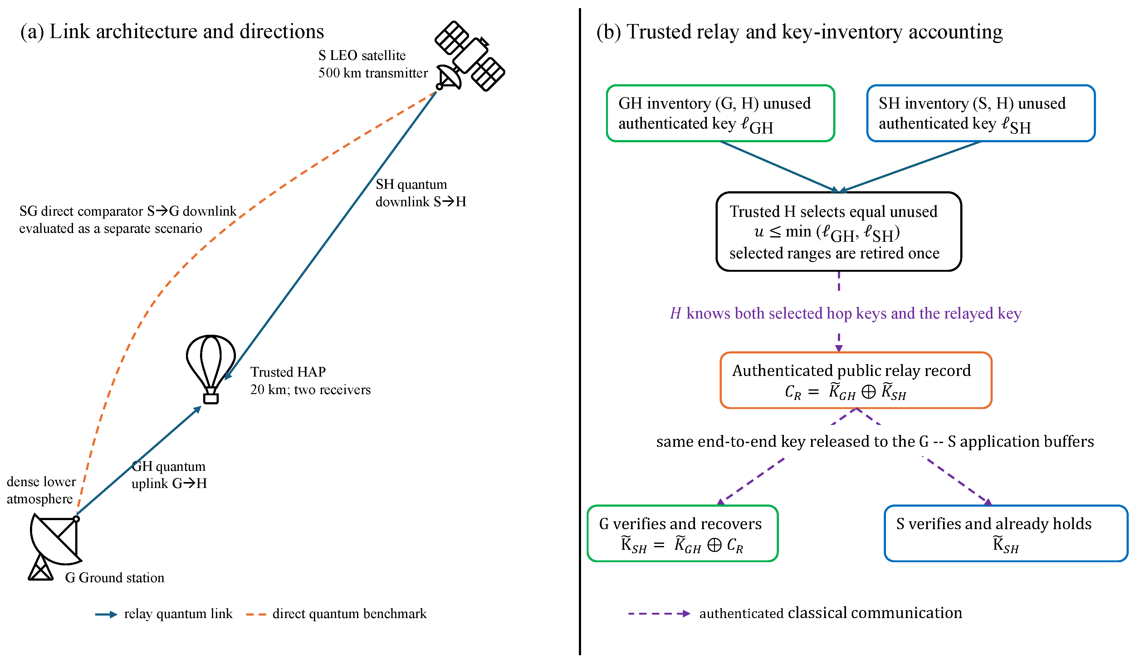
Figure 2.
Reference pass geometry. (a) Satellite elevation observed from the ground station (SG) and HAP (SH), together with the ground and HAP masks. (b) GH, SH, and SG slant ranges. The GH range remains 20 km because the reference HAP is vertically aligned with the ground station.
Figure 2.
Reference pass geometry. (a) Satellite elevation observed from the ground station (SG) and HAP (SH), together with the ground and HAP masks. (b) GH, SH, and SG slant ranges. The GH range remains 20 km because the reference HAP is vertically aligned with the ground station.
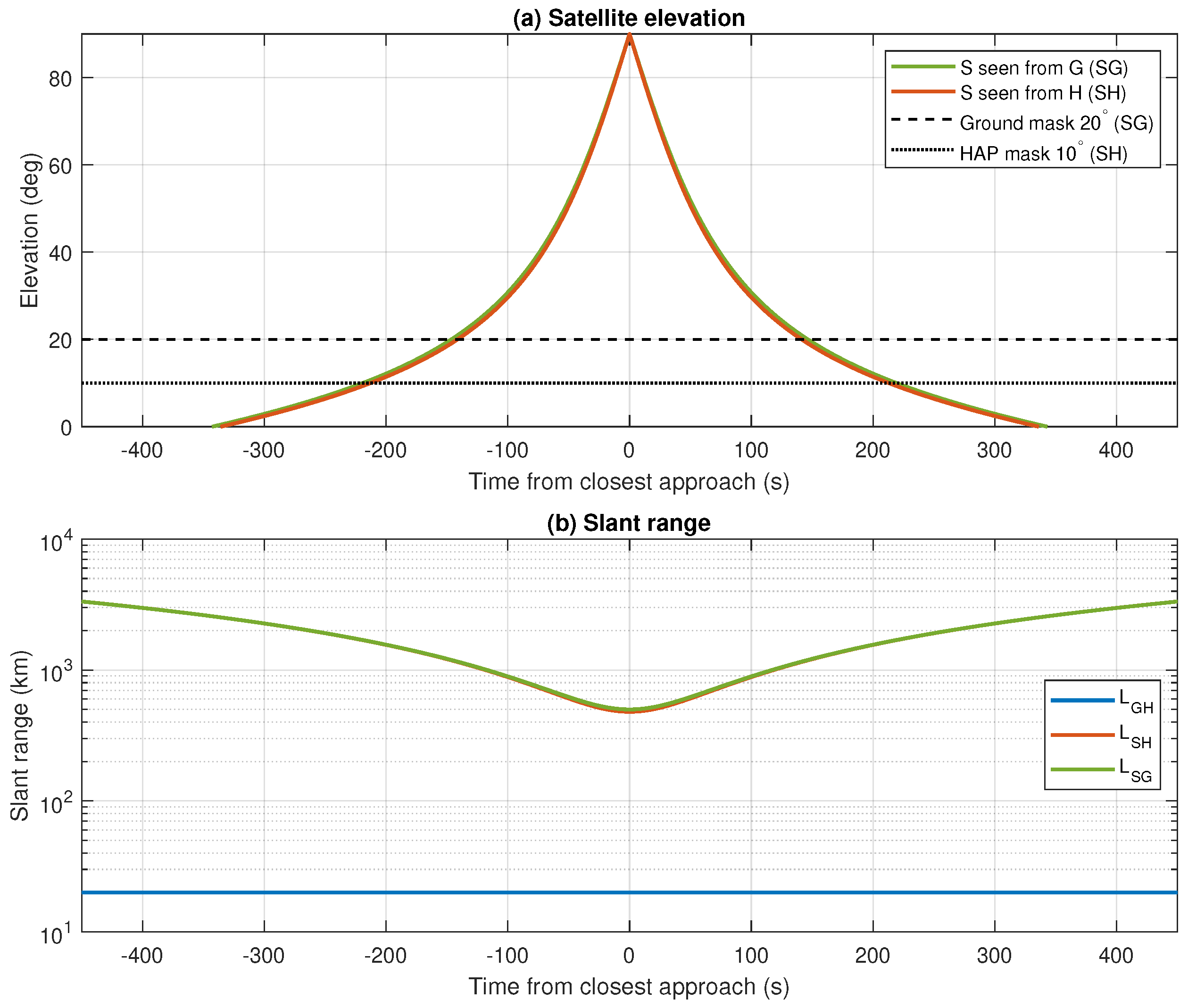
Figure 5.
Secret-key fraction versus emitted block size for stationary pre-detection channel losses of , , and dB using the reference SH/HAP receiver and default protocol. Solid curves use the finite-key estimator with expected counts, Eq. (22); zero-key grid points are omitted from the logarithmic vertical axis. Dashed lines show the corresponding asymptotic estimator, Eq. (23), after removing statistical deviations and additive finite-security penalties.
Figure 5.
Secret-key fraction versus emitted block size for stationary pre-detection channel losses of , , and dB using the reference SH/HAP receiver and default protocol. Solid curves use the finite-key estimator with expected counts, Eq. (22); zero-key grid points are omitted from the logarithmic vertical axis. Dashed lines show the corresponding asymptotic estimator, Eq. (23), after removing statistical deviations and additive finite-security penalties.
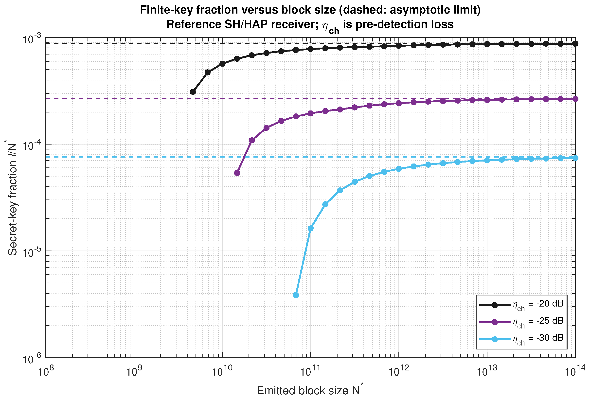
Figure 6.
Master numerical summary. (a) Net link keys versus visibility for the reference HAP radius (solid) and matched HAP radius (dashed). (b) Full-contact trusted-relay and direct S→G downlink yields; a direct G→S uplink is not included. (c) Probability that at least one request is starved during a 200-pass schedule versus application-buffer capacity; solid curves denote the reference/full relay and dashed curves the matched/full relay. The zero-capacity point is displayed at bits solely to permit a logarithmic horizontal axis. (d) Best-so-far simulated-annealing objective, together with the final equal-budget grid and random-search levels and the fixed default. Grid and random-search lines indicate final levels rather than full convergence histories.
Figure 6.
Master numerical summary. (a) Net link keys versus visibility for the reference HAP radius (solid) and matched HAP radius (dashed). (b) Full-contact trusted-relay and direct S→G downlink yields; a direct G→S uplink is not included. (c) Probability that at least one request is starved during a 200-pass schedule versus application-buffer capacity; solid curves denote the reference/full relay and dashed curves the matched/full relay. The zero-capacity point is displayed at bits solely to permit a logarithmic horizontal axis. (d) Best-so-far simulated-annealing objective, together with the final equal-budget grid and random-search levels and the fixed default. Grid and random-search lines indicate final levels rather than full convergence histories.
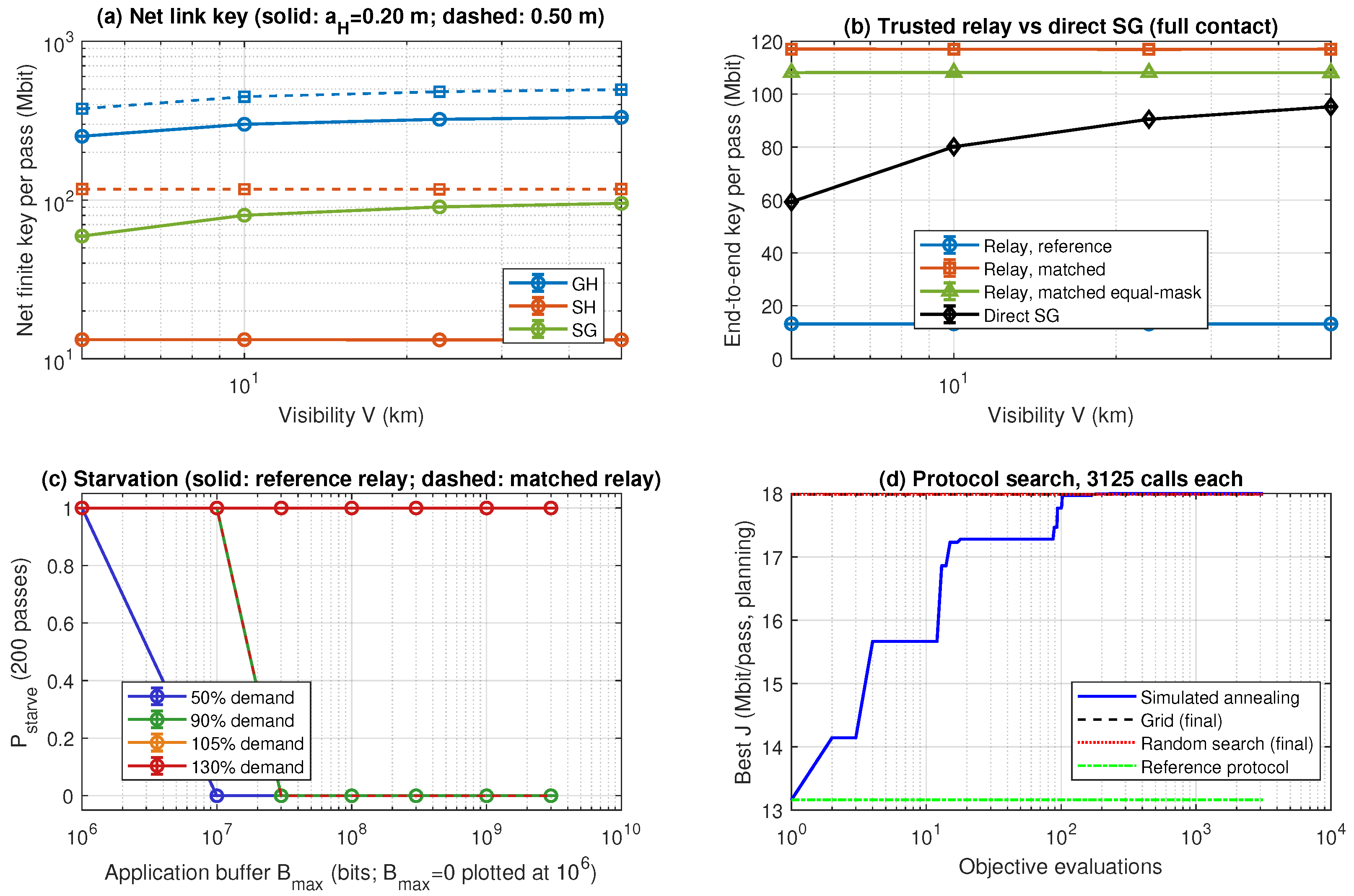
Figure 7.
Weather-weighted end-to-end key at the three tested HAP receive radii. Error bars are 95% Monte Carlo confidence-interval half-widths. The dashed line is the mean of the three sensitivity SG estimates (84.3 Mbit/pass), and the dotted line marks the 0.50 m ground receive radius. The dash-dotted crossing near 0.375 m is a log-radius interpolation between sparse simulated points, included only as a visual guide.
Figure 7.
Weather-weighted end-to-end key at the three tested HAP receive radii. Error bars are 95% Monte Carlo confidence-interval half-widths. The dashed line is the mean of the three sensitivity SG estimates (84.3 Mbit/pass), and the dotted line marks the 0.50 m ground receive radius. The dash-dotted crossing near 0.375 m is a log-radius interpolation between sparse simulated points, included only as a visual guide.
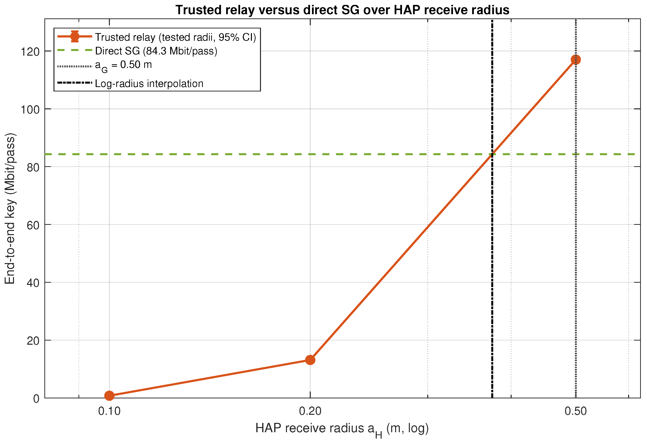
Figure 8.
One-factor sensitivity of the weather-weighted reference/full relay key. Each bar spans the change from the 13.156 Mbit/pass sensitivity baseline over the tested values of one factor, with all other factors held at baseline. Background radiance is expressed in W . The persistence result refers to the selected service operating point and does not imply invariance for every workload and buffer.
Figure 8.
One-factor sensitivity of the weather-weighted reference/full relay key. Each bar spans the change from the 13.156 Mbit/pass sensitivity baseline over the tested values of one factor, with all other factors held at baseline. Background radiance is expressed in W . The persistence result refers to the selected service operating point and does not imply invariance for every workload and buffer.
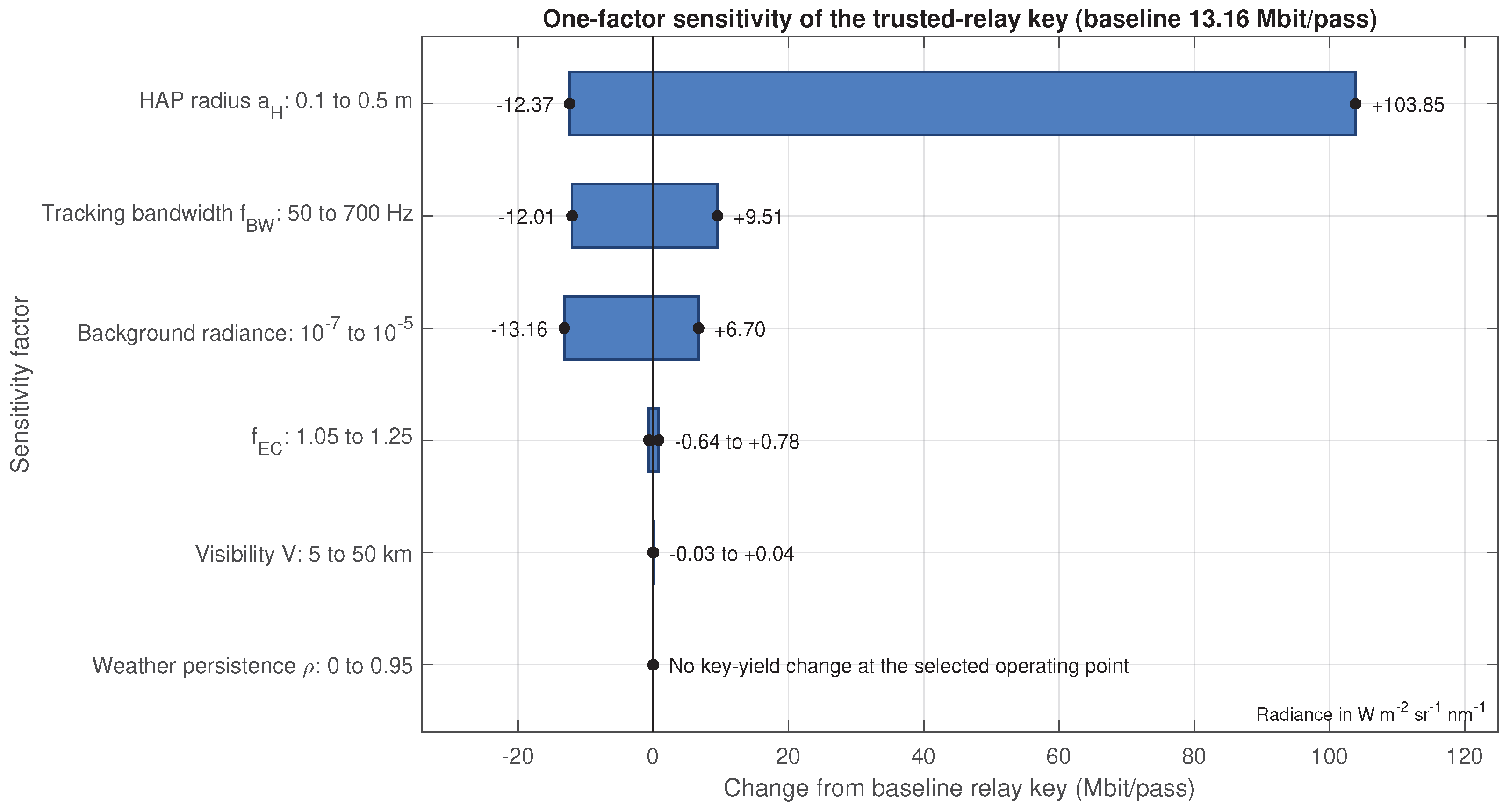
Table 1.
Principal settings used in the numerical evaluation. Receiver, optical, atmospheric, pointing, processing, and numerical inputs are listed in Table A1 (Appendix B).
Table 1.
Principal settings used in the numerical evaluation. Receiver, optical, atmospheric, pointing, processing, and numerical inputs are listed in Table A1 (Appendix B).
| Group | Value |
|---|---|
| HAP altitude; satellite altitude; inclination | 20 km; 500 km; |
| Ground/HAP elevation masks | ; reference or equal-mask |
| Wavelength; ground receive radius | 1550 nm; 0.50 m |
| HAP receive radius | 0.20 m reference; 0.50 m matched |
| Repetition rates | 10 MHz (GH); 500 MHz (SH and SG) |
| Decoy ; | ; |
| Basis and EC ; | ; 1.16 |
| Security | per link block |
| Availability target; lifetime security target | 0.99 per 200-pass horizon; |
| Earth radius; ; rotation rate | 6371 km; ; rad/s |
| Authentication tag length; initial reserve | 128 bits; 65,536 bits per direction |
| Visibility values and probabilities | 5, 10, 23, 50 km; 0.15, 0.25, 0.40, 0.20 |
| Service horizon; schedules; requests | 200 passes; 10,000 schedules; four requests/pass |
| Buffer capacities tested; weather persistence | 0, 10, 30, 100, 300, 1000, 3000 Mbit; |
| Count realizations; generator | 64 per case/link/visibility; MRG32k3a, seed 20260916 |
Table 2.
Evaluated hardware and contact-window cases. Radius denotes the receive-aperture radius applied to both HAP receivers (GH and SH).
Table 2.
Evaluated hardware and contact-window cases. Radius denotes the receive-aperture radius applied to both HAP receivers (GH and SH).
| Case | (m) | HAP mask | Window rule |
|---|---|---|---|
| Reference/full | 0.20 | Each link uses its full contact | |
| Reference/common | 0.20 | Common SG-overlap interval | |
| Matched/full | 0.50 | Each link uses its full contact | |
| Matched/common | 0.50 | Common SG-overlap interval | |
| Matched/equal-mask/full | 0.50 | Each link uses its full contact | |
| Matched/equal-mask/common | 0.50 | Common equal-mask overlap |
Table 3.
Weather-weighted net key per pass. Entries are mean ± 95% Monte Carlo confidence-interval half-width in Mbit/pass. The confidence intervals combine the independently sampled visibility strata in quadrature using their declared probabilities. SG denotes the modeled direct S→G downlink benchmark; a direct G→S uplink is not included.
Table 3.
Weather-weighted net key per pass. Entries are mean ± 95% Monte Carlo confidence-interval half-width in Mbit/pass. The confidence intervals combine the independently sampled visibility strata in quadrature using their declared probabilities. SG denotes the modeled direct S→G downlink benchmark; a direct G→S uplink is not included.
| Case | GH (Mbit/pass) | SH (Mbit/pass) | Relay (Mbit/pass) | SG (Mbit/pass) | Relay/SG |
|---|---|---|---|---|---|
| Reference/full | 0.156 | ||||
| Reference/common | 0.148 | ||||
| Matched/full | 1.388 | ||||
| Matched/common | 1.296 | ||||
| Matched/equal-mask/full | 1.284 | ||||
| Matched/equal-mask/common | 1.293 |
Table 4.
Application-buffer result for the reference/full and matched/full relays. Demand is total demand per pass expressed relative to the weather-weighted reference/full supply and divided among four requests. Infeasible means that no capacity in the tested 0–3000 Mbit sweep reached the 0.99 horizon-availability target (Eq. (33)).
Table 4.
Application-buffer result for the reference/full and matched/full relays. Demand is total demand per pass expressed relative to the weather-weighted reference/full supply and divided among four requests. Infeasible means that no capacity in the tested 0–3000 Mbit sweep reached the 0.99 horizon-availability target (Eq. (33)).
| Relay case | Demand | Smallest successful | Observed starved schedules |
|---|---|---|---|
| Reference/full | 50% | 10 Mbit | 0/10,000 at 10 Mbit |
| Reference/full | 90% | 30 Mbit | 0/10,000 at 30 Mbit |
| Reference/full | 105% | Infeasible through 3000 Mbit | 10,000/10,000 at 3000 Mbit |
| Reference/full | 130% | Infeasible through 3000 Mbit | 10,000/10,000 at 3000 Mbit |
| Matched/full | 50% | 10 Mbit | 0/10,000 at 10 Mbit |
| Matched/full | 90% | 30 Mbit | 0/10,000 at 30 Mbit |
| Matched/full | 105% | 30 Mbit | 0/10,000 at 30 Mbit |
| Matched/full | 130% | 30 Mbit | 0/10,000 at 30 Mbit |
Table 5.
Reference/full protocol search. The last column gives the weather-weighted integer-count mean ± 95% Monte Carlo confidence-interval half-width. All search methods use 3125 calls; the fixed default uses one evaluation.
Table 5.
Reference/full protocol search. The last column gives the weather-weighted integer-count mean ± 95% Monte Carlo confidence-interval half-width. All search methods use 3125 calls; the fixed default uses one evaluation.
| Method | Planning (Mbit/pass) | Reevaluated (Mbit/pass) | |||
|---|---|---|---|---|---|
| Fixed default | 0.500000 | 0.100000 | 0.900000 | 13.163 | |
| Simulated annealing | 0.563183 | 0.263856 | 0.888712 | 17.999 | |
| Grid | 0.566667 | 0.266667 | 0.883750 | 17.986 | |
| Random search | 0.554787 | 0.258929 | 0.884886 | 17.987 |
Disclaimer/Publisher’s Note: The statements, opinions and data contained in all publications are solely those of the individual author(s) and contributor(s) and not of MDPI and/or the editor(s). MDPI and/or the editor(s) disclaim responsibility for any injury to people or property resulting from any ideas, methods, instructions or products referred to in the content. |
© 2026 by the authors. Licensee MDPI, Basel, Switzerland. This article is an open access article distributed under the terms and conditions of the Creative Commons Attribution (CC BY) license (http://creativecommons.org/licenses/by/4.0/).
Copyright: This open access article is published under a Creative Commons CC BY 4.0 license, which permit the free download, distribution, and reuse, provided that the author and preprint are cited in any reuse.