

Submitted:
13 October 2026
Posted:
14 October 2026
You are already at the latest version
Abstract
Rural road planning in mountainous areas must coordinate existing-road use, hierarchical connectivity, and construction requirements. This study proposes a network generation method integrating existing-road topology with roadless space through a hexagonal occupancy grid. Existing-road neighborhood and cross-neighborhood edges represent different access characteristics. Sequential rules generate a county-level backbone, township-level links, and village-level access, while identifying reuse, upgrading, and new construction. Six scenarios are compared in Zhangjiachuan Hui Autonomous County, Gansu, China. The proposed scenario generates an 880.001 km network, with existing roads accounting for 94.53%. New construction totals 48.128 km, 85.63% less than under uniform cross-neighborhood representation. Mean shortest travel times for village-to-township government, township government-to-county seat, and village-to-county seat connections decrease by 15.65%, 37.85%, and 27.91%, respectively, relative to the pre-planning network. All three hierarchical compliance rates reach 100%. The proposed scenario achieves the highest composite score among the six scenarios under the specified indicators and weights, balancing existing-road use, service accessibility, and construction requirements. The method supports preliminary network layouts and scenario comparison in mountainous counties with comparable terrain and road data.
Keywords:
rural road networks
; mountainous terrain
; hexagonal occupancy grid
; hierarchical road-network constraints
; existing road infrastructure utilization
1. Introduction
Rural road networks connect urban and rural trunk transport systems, support local industries, and provide essential access to everyday services. In China, rural revitalization and the initiative to build, manage, maintain, and operate rural roads effectively have reinforced their role in local transport networks [1]. In mountainous areas, the quality of rural road planning and the suitability of network layouts directly affect county-level transport provision and urban–rural integration.
In road network planning and route alignment, spatial representations used for path search include graph models [2], occupancy grids [3], continuous-space models [4], and navigation meshes [5]. Graph models represent a road network as G = (V,E), where V denotes transport nodes and E denotes road segments; edge weights express travel costs [2]. Occupancy grids divide a planning area into regular rectangular, triangular, or hexagonal cells, assign costs from cell attributes, and search through neighboring cells [6,7]. Continuous-space models represent routes as curves rather than discrete graph connections. Routes are optimized through functional optimization or numerical procedures, including genetic algorithms [8,9], particle swarm optimization [10], and hybrid methods [11]. Navigation meshes divide traversable space into irregular convex polygons based on terrain boundaries and obstacles, simplifying collision checks and supporting A* search and its variants [12,13].
For county-level road planning, grid-only representations can have difficulty preserving both existing road geometry and topology. Converting roads into cost cells incorporates road conditions and terrain costs in a common grid [14], but discretization is sensitive to resolution and may introduce positional shifts, discontinuities, or distorted intersections [15,16]. Hybrid road-network and grid graphs retain vector roads and connect them to roadless grid space, enabling searches across both representations [15,17]. Hierarchical county-level planning additionally requires a consistent representation of the connectivity of different road administrative categories, their connections with the grid, and their cost differences. A high-resolution grid can represent the planning area while topological edges retain existing roads and support differentiated connection costs associated with road administrative categories.
Cost models underpin path search and route optimization. Depending on their inputs, costs can be classified as spatial-state-dependent, local-transition-dependent, or cumulative-state-dependent. Spatial-state-dependent costs reflect location-specific properties such as land use, ecological sensitivity, geological hazards, and land cover [18]. Local-transition-dependent costs represent movement between neighboring locations, including distance, gradient, travel direction, curvature, and engineering quantities [19,20]. Cumulative-state-dependent costs depend on the path already formed and its history, including changes in direction, resource consumption, and road utilization states [21]. Road planning commonly combines these components in a composite cost model.
County-, township-, and village-level nodes differ in service coverage and passenger and freight requirements. Rural road planning therefore extends beyond generating individual low-cost segments to organizing a hierarchical network. County roads provide county-wide connections, township roads support local distribution, and village roads provide access to settlements. Planning must connect functional nodes, avoid no-build areas, use existing infrastructure, and coordinate connections between road levels. Relevant approaches include hierarchical network design, terrain-constrained hierarchical road generation, and simulations of hierarchical network evolution. Hierarchical network design uses abstract nodes and candidate connections, organizing backbones and branches through node classification, minimum spanning trees, and multilevel optimization [22,23]. Terrain-constrained generation assigns road levels and connection tasks according to settlement size, road type, or specified endpoints, then searches for alignments using terrain costs [16,24]. Evolutionary models simulate traffic assignment and investment updates based on demand, benefits, construction costs, and changing road performance to explain emerging road and hub hierarchies [25]. These approaches organize networks using node levels, candidate links, settlement size, or endpoint type. County boundaries, township affiliation, service functions, and permitted interlevel connections require more explicit treatment to ensure that county, township, and village roads serve their intended areas and functions. Administrative affiliation, node levels, search extents, permitted access targets, and no-build areas must therefore be translated into explicit network generation constraints.
Existing-road use can be represented through static low-cost guidance, condition-specific costing, and sequential network reuse. Static guidance assigns zero costs, low costs, or off-road distance costs to existing roads and nearby areas to encourage their use [14,16]. Condition-specific costing distinguishes direct reuse, maintenance, upgrading, reconstruction, and new construction according to road class, pavement condition, and required engineering works [19,26]. Sequential reuse incorporates existing and previously generated roads into the current network and reduces subsequent access or travel costs, encouraging later routes to share infrastructure [14,27,28]. Hybrid road-topology and traversable-space representations further treat existing roads as a backbone with low incremental construction costs, connected to regular grid cells or irregular traversable units through neighborhood relations [15,27]. These approaches support preferential use of existing infrastructure, but further attention is needed to identify how planned routes correspond to reuse, upgrading, and new construction.
This study makes three contributions. First, it integrates existing-road topology with roadless space by representing roads as neighborhood or cross-neighborhood edges according to their administrative categories and access characteristics, allowing infrastructure reuse and new-corridor search in one graph. Second, it translates county-level continuity, township-level links, and village access within the assigned township into hierarchical constraints and sequential network updates, generating a county-level backbone, township-level links, and village-level access. Third, it identifies reuse, upgrading, and new construction during network generation using road origin, target hierarchy, and utilization state, supporting subsequent evaluation of infrastructure use and construction requirements.
2. Materials and Methods
2.1. Study Area and Data
Zhangjiachuan Hui Autonomous County is located in southeastern Gansu Province, China, at the transition between the Liupan Mountains and the Longxi Loess Plateau (Figure 1). The county covers approximately 1311.8 km2, with a mean elevation of 2011.4 m and an elevation range of 1173.4 m. Terrain relief is generally greater in the northeast and lower in the central and western parts. This varied topography strongly constrains rural road layouts and construction costs. The study uses a digital elevation model (DEM), administrative boundaries, existing roads, county-, township-, and village-level planning nodes, and no-build areas (Table 1).
The workflow comprises six steps: data alignment, integrated representation of the hexagonal occupancy grid and existing roads, composite edge-cost calculation, sequential county–township–village network generation, identification of road construction types, and evaluation of the planning results (Figure 2).
2.2. Construction of the Hexagonal Occupancy Grid
A regular hexagonal tessellation with a fixed coordinate origin is generated within the county boundary [29]. Cells in no-build areas are removed to obtain the basic spatial units (Figure 3). Each regular hexagon has six equidistant neighboring centers, providing six expansion directions with a common adjacency distance rather than the two-axis restriction of a four-neighbor square grid. Low-category roads predominate in the study area (Figure 4), and 89% of road widths lie between 3.5 and 5.5 m. A hexagon side length of 5 m is used for the case-study planning representation.
Grid attributes describe geometric indexing, terrain, administrative affiliation, area status, and adjacency. Table 2 summarizes the principal attributes and assignment methods.
2.3. Integrated Representation of Existing-Road Topology and Roadless Space
Hexagon centers serve as nodes, and grid neighborhood edges form the basic search graph. Existing roads are represented by existing-road neighborhood edges or existing-road cross-neighborhood edges according to road administrative category and access rules (Figure 5). Cross-neighborhood edges connect nonadjacent nodes and may traverse multiple hexagons, whereas neighborhood edges represent road segments between consecutive access locations along a road. Expressway cross-neighborhood edges connect grid nodes containing road endpoints or entrances and exits. National and provincial roads are divided into continuous segments between nodes containing endpoints, connected intersections, or attribute-change locations. County, township, and village roads are matched to the grid nodes along their alignments to form neighborhood edges.
Figure 5a shows the spatial relationship between existing roads and the hexagonal grid. Figure 5b illustrates the integrated graph formed by grid nodes, grid neighborhood edges, existing-road neighborhood edges, and cross-neighborhood edges over three-dimensional terrain.
The grid-center nodes and three edge types form the integrated road-network graph:
G = (VH,EH ∪ EA∪ER) (1)
2.4. Edge-Cost Calculation
Relative incremental construction costs represent differences in the investment required during network generation. They depend on distance, gradient, and construction types and do not directly represent monetary engineering costs. Direct reuse means that an existing road can serve the current connection task without modification; its incremental construction cost is therefore zero. Upgrading requires engineering works, and its cost is expressed as a proportion of the cost of new construction under equivalent target conditions.
The cost of a grid neighborhood edge is based on the slope-class least-cost model proposed by Yu et al. [30]. For adjacent nodes with three-dimensional coordinates (xi,yi,zi) and (xj,yj,zj), the directional slope angle is:
(2)
where the horizontal distance Lij is:
(3)
Slope magnitudes are assigned to five finite-cost classes, with an additional excluded range [30]:
(4)
Spatial distance Dij, the mean basic cost of adjacent cells , and the slope weight ω(|θij|) are combined to obtain the local cost of grid neighborhood edge ij:
(5)
where the three-dimensional distance Dij is:
(6)
Here, is the mean basic cell cost at the two endpoints of the grid neighborhood edge [30].
Existing-road neighborhood edges have two construction states: reuse and upgrading. Reuse incurs no incremental construction cost, giving cE = 0. Upgrading improves the road’s technical condition before use, and its cost is calculated as:
(7)
where is the new-construction reference cost calculated using Equation (5) for the corresponding grid neighborhood edge, and ρu is the upgrading cost coefficient.
Existing-road cross-neighborhood edges are directly reused, with cE = 0.
Path search first minimizes cumulative incremental construction cost. If candidate paths have equal cumulative costs, their actual lengths provide a secondary criterion, and the shorter path is selected.
2.5. Road Network Generation under Hierarchical Constraints
The network is generated sequentially as a county-level backbone, township-level links, and village-level access roads (Figure 6).
During county-level backbone generation, existing-road neighborhood edges below the county-road administrative category receive upgrading costs according to Equation (7); the remaining existing-road neighborhood edges receive reuse costs. After this update, grid neighborhood edges and both types of existing-road edges form the candidate search network. Shortest-path search produces the minimum cumulative cost matrix between county-level planning nodes. An open traveling salesman problem (OTSP) [31,32] determines their connection order, and the corresponding paths form the county-level backbone.
During township-level link generation, the county-level backbone and the roads newly constructed or upgraded in the previous stage are incorporated into the current network, and their edge costs are updated to reuse costs. Existing-road neighborhood edges below the township-road administrative category receive upgrading costs; other existing-road neighborhood edges receive reuse costs. Pairwise costs between township-level planning nodes are recalculated on the updated graph, and the OTSP [31,32] organizes the township-level links.
During village-level access generation, the county–township backbone and all existing-road neighborhood edges are assigned reuse costs. Village-level planning nodes are grouped by township. Each group contains the village nodes of that township and eligible anchor points on the county- and township-level backbone. A rooted minimum spanning tree (MST) [33,34], with the backbone serving as the root, organizes the final access paths.
Construction types are recordedduring sequential generation. Existing-road neighborhood edges requiring no modification are classified as reuse, those requiring improvement to the target level as upgrading, and selected grid neighborhood edges in roadless space as new construction. Selected existing-road cross-neighborhood edges are classified as reuse.When a previously generated segment is used in a later stage, only its search cost is updated; its recorded construction type is retained.
2.6. Evaluation Indicators
The evaluation system covers network composition, service accessibility, and construction requirements (Table 5). Hierarchical compliance is reported separately as a reference. Scored indicators are normalized according to their direction of preference and aggregated using the specified weights.
3. Experiments and Results
3.1. Experimental Design
A baseline scenario is defined for the complex terrain and multiple road administrative categories in Zhangjiachuan Hui Autonomous County, with . Six scenarios combine existing-road representation strategies, R (Table 6), network organization strategies, H (Table 7), and edge-cost settings, K (Table 8), as summarized in Table 9. The scenarios examine the effects of these three components. Global MST and global OTSP serve as network organization comparisons without hierarchical differentiation; the hierarchical MST strategy provides a comparison under the same hierarchical constraints; and the uniform-cost strategy examines the effect of distinguishing construction states in edge costing.
In Table 8, LE is the length of the corresponding existing-road edge, measured in the same units as in the new-construction cost model. The coefficient 0.04 specifies the relative cost per unit length of an existing-road neighborhood edge. It defines a uniform low-cost comparison to examine the effects of not distinguishing reuse from upgrading on network length, service accessibility, and new construction. This dimensionless coefficient does not represent a local monetary construction rate.
3.2. Network Composition
E2 produces a final road network of 880.001 km, comprising 831.873 km of existing roads and 48.128 km of new construction; existing roads account for 94.53% (Table 10). Relative to E1, E2 reduces total length by 113.150 km and new construction by 286.732 km. E5 has the shortest total network, at 525.078 km, but requires 262.601 km of new construction, with existing roads accounting for only 49.99%. E3 has the least new construction, at 41.130 km.
3.3. Improvements in Service Accessibility
Service accessibility is evaluated using the same 523 fixed origin–destination (OD) pairs: 254 village-to-township government pairs, 15 township government-to-county seat pairs, and 254 village-to-county seat pairs. Pre-planning travel times are calculated on the existing road network, whereas post-planning times are calculated on the network consisting of the actual road segments selected by each scenario. The same OD set, length measurement method, and road administrative category speed rules are used for comparability. Following Chen et al. [35], assigned speeds are 100, 80, 60, 40, and 30 km/h for expressways, national roads, provincial roads, county roads, and township/village roads, respectively; other local roads are assigned 30 km/h. Reused roads retain the speed associated with their current road administrative category, while new or upgraded roads receive the speed of their target road administrative category. Mean shortest travel times are calculated for the three service types.
E5 has the shortest times for all three service types: 8.321, 22.994, and 25.645 min (Table 11). The corresponding E2 times are 11.635, 24.463, and 29.372 min, representing improvements of 15.65%, 37.85%, and 27.91% relative to the pre-planning network. E3 increases village-to-township government travel time, yielding a −10.10% improvement, while E6 has a −4.33% improvement for village-to-county seat travel. All other improvement rates are positive. Compared with E6 under the same hierarchical constraints, E2 reduces the three travel times by 0.819, 13.145, and 13.133 min.
3.4. Hierarchical Compliance
E1, E2, E5, and E6 achieve 100% compliance at all three levels, with no prohibited interlevel connections (Table 12). E3 (global MST) and E4 (global OTSP) achieve 100% village-to-assigned-township compliance, but both have a county-level continuity rate of 28.57%; their township-level access compliance rates are 5.26% and 36.84%, respectively. They therefore do not satisfy all predefined functional requirements. Overall connectivity cannot substitute for county- and township-level backbone organization and the prescribed access relationships.
3.5. Construction Types
Table 13 reports reuse, upgrading, and new-construction lengths. E2 includes 825.141 km of reuse, 6.732 km of upgrading, and 48.128 km of new construction, yielding a construction requirements index of 0.0593. E3 has the lowest index (0.0516), whereas E5 has the highest (0.5353). E2 requires 214.473 km less new construction than E5, a reduction of 81.67%, but has longer service travel times, illustrating the trade-off between new construction and accessibility.
3.6. Composite Evaluation
Composite scores compare the six scenarios in terms of network composition, service accessibility, and construction requirements. Hierarchical compliance is reported independently and excluded from the score. The scores therefore reflect the selected indicators and weights and do not replace verification of the hierarchical requirements.
E2 achieves the highest composite score of 76.72, followed by E4 and E3 at 74.58 and 67.48, respectively (Table 14). Its scores for network composition, service accessibility, and construction requirements are 61.67, 73.19, and 98.41. Although E2 does not lead any individual category, it achieves the highest weighted total. E3 and E4 form connected networks but have low county-level continuity and township-level access compliance, and thus do not meet the full functional requirements. E5 has the highest accessibility score but a construction requirements score of zero. E1 has a relatively high accessibility score but lower network-composition and construction requirements scores.
Under the specified indicators, normalization procedures, and weights, E2 has the highest score among the six scenarios and satisfies all three hierarchical requirements. Its results indicate a favorable balance between existing-road use, service accessibility, and construction requirements in this case study. Figure 7 compares local network layouts.
The local layouts reveal differences in existing-road use and node organization (Figure 7). Green segments indicate new construction, while purple segments indicate upgrading of existing roads. E1 and E5 contain more extensive new links across roadless areas. In contrast, E2 relies mainly on existing roads, with localized upgrading and limited new construction to complete the required connections. Upgrading retains existing alignments while improving their technical conditions, whereas new construction provides connections where existing roads are insufficient. Combined with the network-wide results, E2 satisfies the hierarchical requirements that E3 and E4 do not fully meet and achieves shorter average travel times than E6 for all three service categories. These results illustrate how E2 combines existing-road reuse, selective upgrading, and limited new construction to support hierarchical connectivity and service accessibility.
4. Discussion
4.1. Applicability and Trade-Offs
The highest composite score of E2 reflects the combined effects of three components. First, R2 represents higher-category roads with cross-neighborhood edges and lower-category roads with neighborhood edges, incorporating existing infrastructure into the candidate graph. E2 uses 831.873 km of existing roads through reuse and upgrading, substantially more than E1 and E5. Second, sequential county–township–village organization in H2 avoids the hierarchical deficiencies observed in the global strategies E3 and E4. Third, K1 distinguishes reuse from upgrading costs, enabling a trade-off between existing-road use and new construction. E5 has the shortest service travel times but the highest construction requirements index and the lowest use of existing road resources, illustrating the greater new-construction requirement associated with its accessibility gains.
Network organization affects both service accessibility and functional structure. E2 and E6 use the same access and cost rules. With only 1.79% more network length, E2 reduces the three service travel times by 6.58%, 34.95%, and 30.90%, respectively. E3 and E4 have no isolated nodes, yet both attain only 28.57% county-level continuity. These results support treating hierarchical functional requirements as explicit planning priorities rather than relying on overall connectivity or minimum total length.
Global connectivity alone does not ensure a continuous county-level backbone or appropriate township links. In this case, the scenario with the shortest service travel times also requires substantial new construction. By incorporating road functions, administrative affiliation, and existing-road use into generation, the proposed method supports comparison across functional organization, service accessibility, and construction requirements rather than a single length or cost measure. It translates rural road planning requirements into executable network generation rules for constructing and comparing candidate networks in mountainous counties.
4.2. Sensitivity to the Upgrading Cost Coefficient
Sensitivity to the upgrading cost coefficient ρu is examined using values of 0.4, 0.6, and 0.8 while holding the baseline terrain costs, access strategy, and hierarchical constraints fixed. Within each parameter setting, rankings are compared among scenarios satisfying permitted access, hierarchical requirements, and full OD reachability (Table 15).
At upgrading cost coefficients of 0.4, 0.6, and 0.8, the existing-road shares of E2 are 96.02%, 94.53%, and 92.58%, respectively. E2 ranks first in each tested setting, indicating that its recommendation is unchanged within this range. The decreasing existing-road share as the coefficient rises reflects the response of path selection to the assumed upgrading cost.
4.3. Implications for Sustainable Rural Transport Planning
Integrating existing-road use into network generation helps identify opportunities to improve county-wide connections through existing infrastructure. In this case, existing roads account for 94.53% of the proposed network, and new construction is reduced by 286.732 km relative to the uniform cross-neighborhood scenario. This demonstrates the planning value of infrastructure reuse in controlling new road requirements. New-construction length directly indicates the scale of additional road provision; land take, material consumption, and carbon emissions require further quantification using road widths, engineering structures, and construction conditions.
County-level continuity, township-level links, and village access within the assigned township provide a basis for functional connections between service nodes at different levels. The three travel-time indicators describe support for access to administrative services. They provide a foundation for further public-service accessibility analysis incorporating population, vulnerable groups, and facility capacity to examine differences in benefits among residents.
5. Conclusions and Outlook
This study develops a rural road network generation method for mountainous areas under hierarchical constraints. An integrated representation of existing-road topology and roadless space brings infrastructure reuse and new-corridor search into one computational process. County-level continuity, township-level links, and village access within the assigned township are translated into sequential generation rules. Reuse, upgrading, and new construction are identified during generation, allowing the planning output to describe spatial layout, hierarchical functions, and construction requirements together.
Six comparative scenarios in Zhangjiachuan Hui Autonomous County examine existing-road access, network organization, and road-cost settings. The proposed scenario satisfies the predefined hierarchical requirements and achieves the highest composite score under the study’s evaluation system, demonstrating a favorable balance between existing infrastructure use, service accessibility, and new construction.
Future work can extend the framework with travel-demand and regional-development information to support network generation and comparison under additional planning scenarios. Incorporating engineering and material costs can strengthen links with route design and construction scheduling, supporting phased development and continuing improvement of rural roads in mountainous areas.
Author Contributions
Conceptualization and methodology, L.L., Y.X., and P.X.; data analysis and validation, Z.W., H.Z., and P.X.; writing—original draft preparation, L.L. and P.X.; writing—review and editing, all authors. All authors have read and agreed to the published version of the manuscript.
Funding
This work was supported by the National Key R&D Program of China (grant number 2024YFC3808904).
Data Availability Statement
The data supporting the findings of this study are available from the corresponding authors upon reasonable request, subject to applicable data licensing and access restrictions.
Conflicts of Interest
The authors declare no conflicts of interest.
References
- Zhang, X. Rural Revitalization Strategy “four good rural road” Construction Some Thoughts on Gansu PracticeZ. Gansu Sci. Technol. 2020, 36, 7–8. [Google Scholar] [CrossRef]
- Ge, Y.; Wang, J.; Meng, Y.; et al. Research progress on dynamic route planning of vehicle navigation[J]. J. Highw. Transp. Res. Dev. 2010, 27(11), 113–117. [Google Scholar]
- Elfes, A. Using occupancy grids for mobile robot perception and navigation. Computer 1989, 22, 46–57. [Google Scholar] [CrossRef]
- Yershov, D.S.; LaValle, S.M. Simplicial Dijkstra and A* algorithms: From graphs to continuous spaces. Adv. Robot. 2012, 26, 2065–2085. [Google Scholar] [CrossRef]
- Cao, L.; RAO, Z.; HE, Y. 3D Space Representation Using Navigation Meshes, J[J]. J. Syst. Simul. 2008, 20(9), 232–234. [Google Scholar]
- Zhang, Z.; Zhang, J.; Zhao, Y.; et al. A novel hexagonal grid map model and regenerated heuristic factor based strategy for intelligent manufacturing system’s AGV path planning problem solving. Comput. Ind. Eng. 2024, 192, 110154. [Google Scholar] [CrossRef]
- Zhang, J.; Wang, X.; Xu, L.; et al. An occupancy information grid model for path planning of intelligent robots. ISPRS Int. J. Geo-Inf. 2022, 11, 231. [Google Scholar] [CrossRef]
- Caihong, L.; Jiquan, H.; Xiaoning, Q. Path Design of Robot Within Continuous Space Based on Hybrid Genetic Algorithms[J]. J.-WUHAN Transp. Univ. 2003, 27(6), 819–821. [Google Scholar]
- Nazarahari, M.; Khanmirza, E.; Doostie, S. Multi-objective multi-robot path planning in continuous environment using an enhanced genetic algorithm. Expert Syst. With Appl. 2019, 115, 106–120. [Google Scholar] [CrossRef]
- Bin, L.I.U.; Ren-jin, Z.H.A.N.G. A path planning method using two-stage particle swarm optimization[J]. J. SHANDONG Univ. (ENGINEERING SCIENCE) 2012, 42(1), 12–18. [Google Scholar]
- Dong, G.; Zhao, F.; Zhuo, J.; et al. Topological progress potential-enhanced continuous-space ant colony algorithm for robot path planning. Sensors 2026, 26, 1264. [Google Scholar] [CrossRef] [PubMed]
- Wuping, L.I.U.; Weiqian, X.I.O.N.G. An Indoor Path Planning Algorithm Based on Multi-layer Navigation Grid. J. Geomat. 2020, 45(6), 18–21. [Google Scholar] [CrossRef]
- Tian, T.; Wu, H.; Wei, H.; et al. An efficient path planning algorithm based on Delaunay triangular NavMesh for off-road vehicle navigation. World Electr. Veh. J. 2025, 16, 382. [Google Scholar] [CrossRef]
- Hughes, J.; Endicott, S.; Lapins, D.; et al. Development and assessment of automated forest road projection methods using performance metrics relevant for wildlife. Landsc. Ecol. 2025, 40, 208. [Google Scholar] [CrossRef]
- Choi, Y.; Um, J.G.; Park, M.H. Finding least-cost paths across a continuous raster surface with discrete vector networks. Cartogr. Geogr. Inf. Sci. 2014, 41, 75–85. [Google Scholar] [CrossRef]
- Liu, Y.; Bao, S.; She, M.; et al. Intelligent Planning of Village Roads for Rural Revitalization: A Case Study of Gangtou Village, Huadu District, Guangzhou[J]. Trop. Geogr. 2023, 43(2), 226–233. [Google Scholar]
- Wu, Z.; Zhang, H.; Zhang, Z.; et al. Global path planning methods based on the relationship between traversability capability and terrain matching. Sensors 2026, 26, 1472. [Google Scholar] [CrossRef] [PubMed]
- Atkinson, D.M.; Deadman, P.; Dudycha, D.; et al. Multi-criteria evaluation and least cost path analysis for an arctic all-weather road. Appl. Geogr. 2005, 25, 287–307. [Google Scholar]
- Mahanpoor, M.; Monajjem, S.; Balali, V. An optimization model for synchronous road geometric and pavement enhancements. J. Traffic Transp. Eng. (English Edition) 2021, 8, 421–438. [Google Scholar] [CrossRef]
- Collischonn, W.; Pilar, J.V. A direction dependent least-cost-path algorithm for roads and canals. Int. J. Geogr. Inf. Sci. 2000, 14, 397–406. [Google Scholar] [CrossRef]
- Wallin, E.; Wiberg, V.; Vesterlund, F.; et al. Learning multiobjective rough terrain traversability. J. Terramechanics 2022, 102, 17–26. [Google Scholar] [CrossRef]
- Current, J.R.; ReVelle, C.S.; Cohon, J.L. The hierarchical network design problem. Eur. J. Oper. Res. 1986, 27, 57–66. [Google Scholar] [CrossRef]
- Yu-long, P.E.I.; chong, Y.U.-W.E.N.; Jing, L.I.U.; et al. Layout method of main arterial highway network based on comprehensive transportation concept[J]. J. Jilin Univ. (Engineering and Technology Edition) 2023, 53(11), 3078–3087. [Google Scholar] [CrossRef]
- Galin, E.; Peytavie, A.; Guérin, E.; et al. Authoring hierarchical road networks. Comput. Graph. Forum 2011, 30, 2021–2030. [Google Scholar] [CrossRef]
- Louf, R.; Jensen, P.; Barthelemy, M. Emergence of hierarchy in cost-driven growth of spatial networks. Proc. Natl. Acad. Sci. 2013, 110, 8824–8829. [Google Scholar] [CrossRef] [PubMed]
- Papageorgiou, G.; Mouratidis, A.; Eliou, N. Comprehensive model for upgrading two-lane road network. Eur. Transp. Res. Rev. 2012, 4, 125–135. [Google Scholar] [CrossRef]
- Hardy, C.; Messier, C.; Valeria, O.; et al. A LANDIS-II extension for simulating forest road networks. Can. J. For. Res. 2023, 53, 503–518. [Google Scholar] [CrossRef]
- Stahlberg, M.J.; Sagnol, G.; Ducke, B.; et al. Spatiotemporal reconstruction of ancient road networks through sequential cost–benefit analysis. PNAS Nexus 2023, 2, pgac313. [Google Scholar] [CrossRef] [PubMed]
- Wang, L.; Ai, T.; Shen, Y.; et al. The isotropic organization of DEM structure and extraction of valley lines using hexagonal grid. Trans. GIS 2020, 24, 483–507. [Google Scholar] [CrossRef]
- Yu, C.; Lee, J.; Munro-Stasiuk, M.J. Extensions to least-cost path algorithms for roadway planning. Int. J. Geogr. Inf. Sci. 2003, 17, 361–376. [Google Scholar] [CrossRef]
- Lam, F.; Newman, A. Traveling salesman path problems. Math. Program. 2008, 113, 39–59. [Google Scholar] [CrossRef]
- Sengupta, L.; Mariescu-Istodor, R.; Fränti, P. Which local search operator works best for the open-loop TSP? Appl. Sci. 2019, 9, 3985. [Google Scholar] [CrossRef]
- Kruskal, J.B. On the shortest spanning subtree of a graph and the traveling salesman problem. Proc. Am. Math. Soc. 1956, 7, 48–50. [Google Scholar] [CrossRef]
- Shrestha, J.K.; Benta, A.; Lopes, R.B.; et al. Covering-based rural road network methodology for hilly regions of developing countries: Application in Nepal. J. Transp. Eng. Part A Syst. 2017, 143, 04016010. [Google Scholar] [CrossRef]
- Chen, S. T.; Li, Y. R.; Pan, W.; et al. Evolution of China’s overland transportation dominance and its economic effect: A county-level analysis[J]. Acta Geogr. Sin. 2022, 77, 1937–1952. [Google Scholar]
Figure 1.
Location and existing road network of Zhangjiachuan Hui Autonomous County.
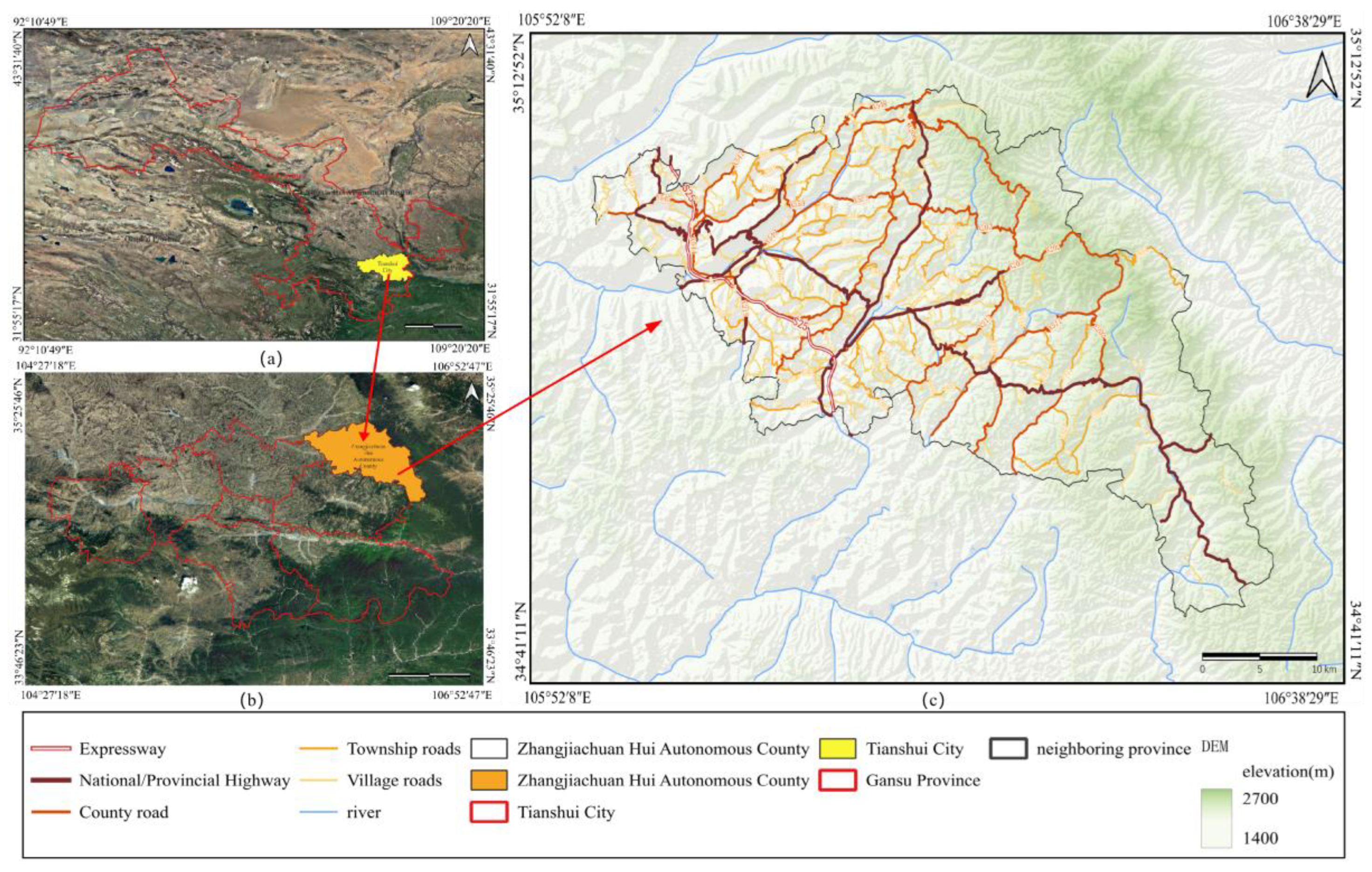
Figure 2.
Methodological workflow.
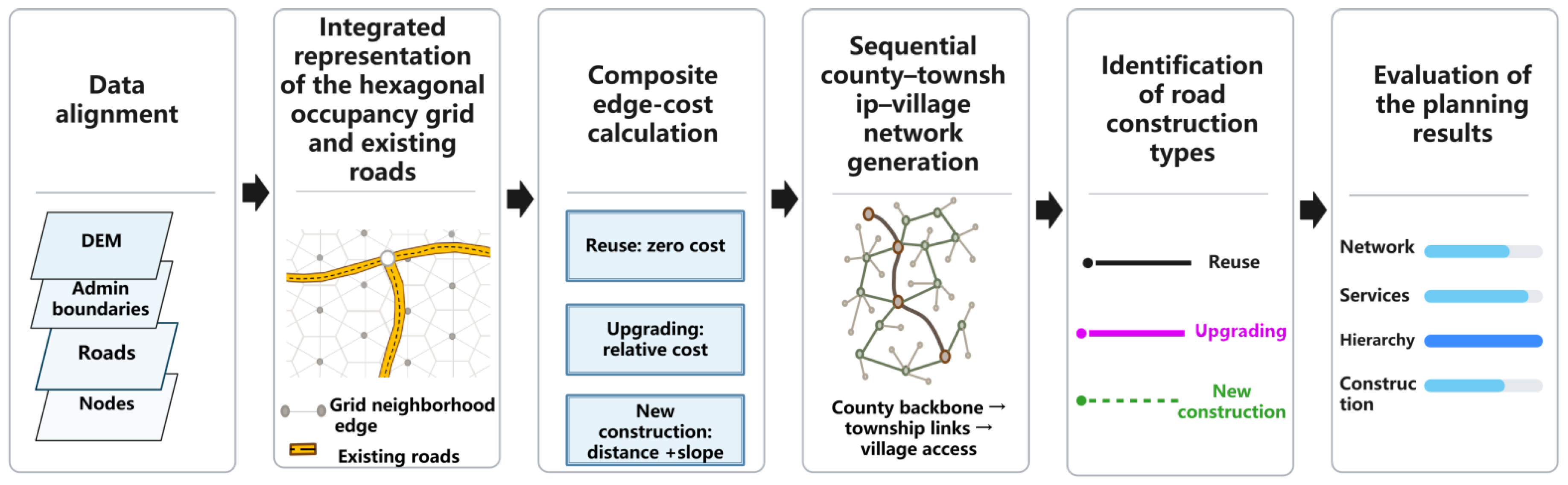
Figure 3.
Hexagonal occupancy grid.
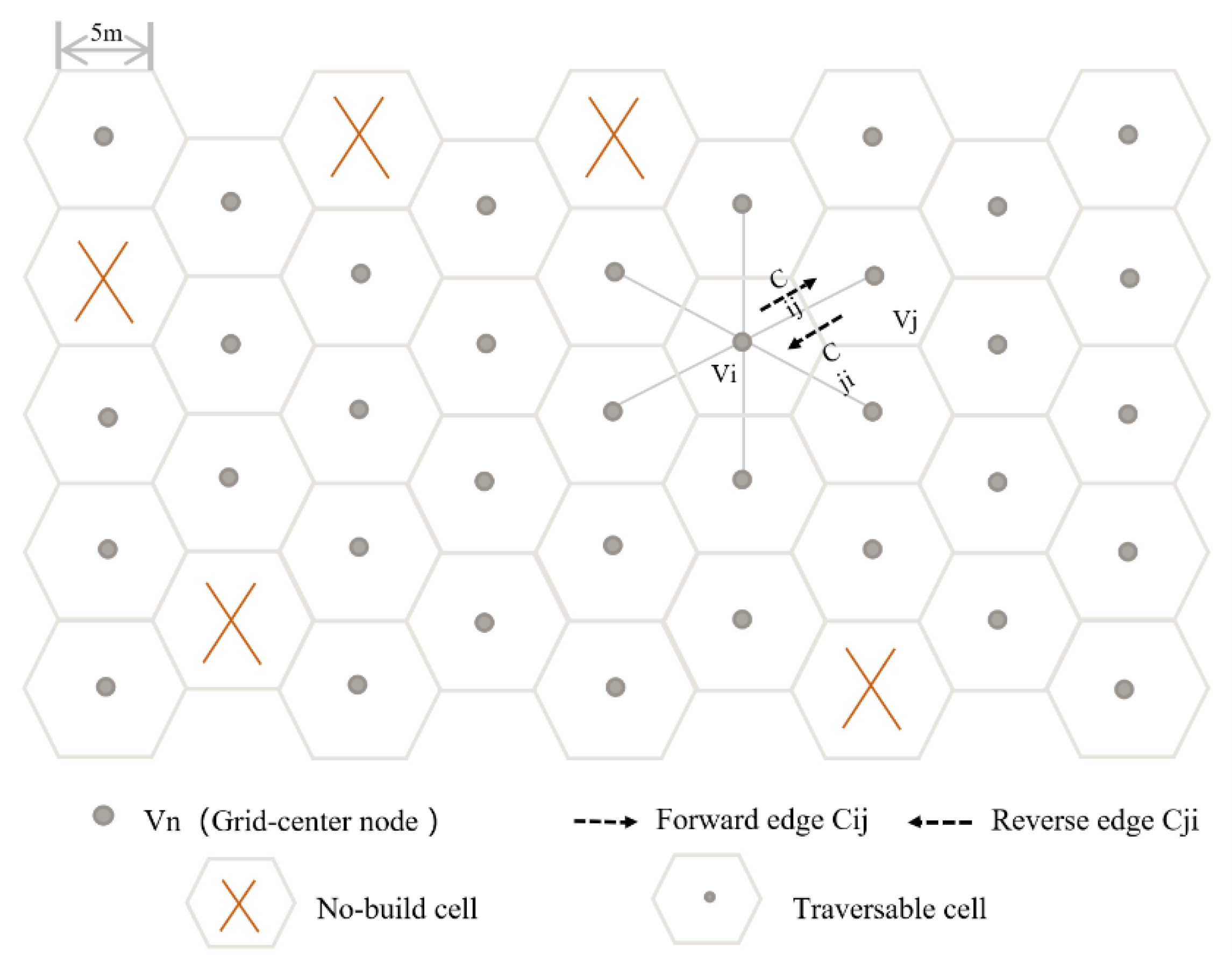
Figure 4.
Width distribution of county, township, and village roads.
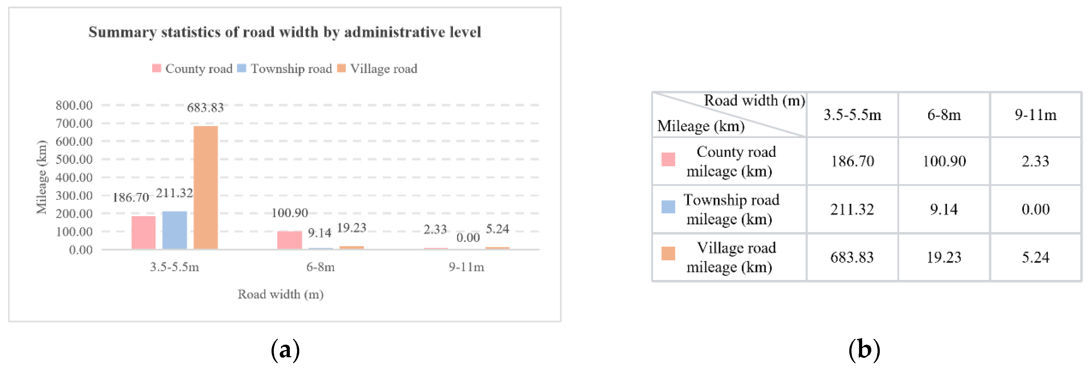
Figure 5.
Integrated road-network representation: (a) existing roads overlaid on the hexagonal grid; (b) the grid and existing-road edges over three-dimensional terrain.
Figure 5.
Integrated road-network representation: (a) existing roads overlaid on the hexagonal grid; (b) the grid and existing-road edges over three-dimensional terrain.
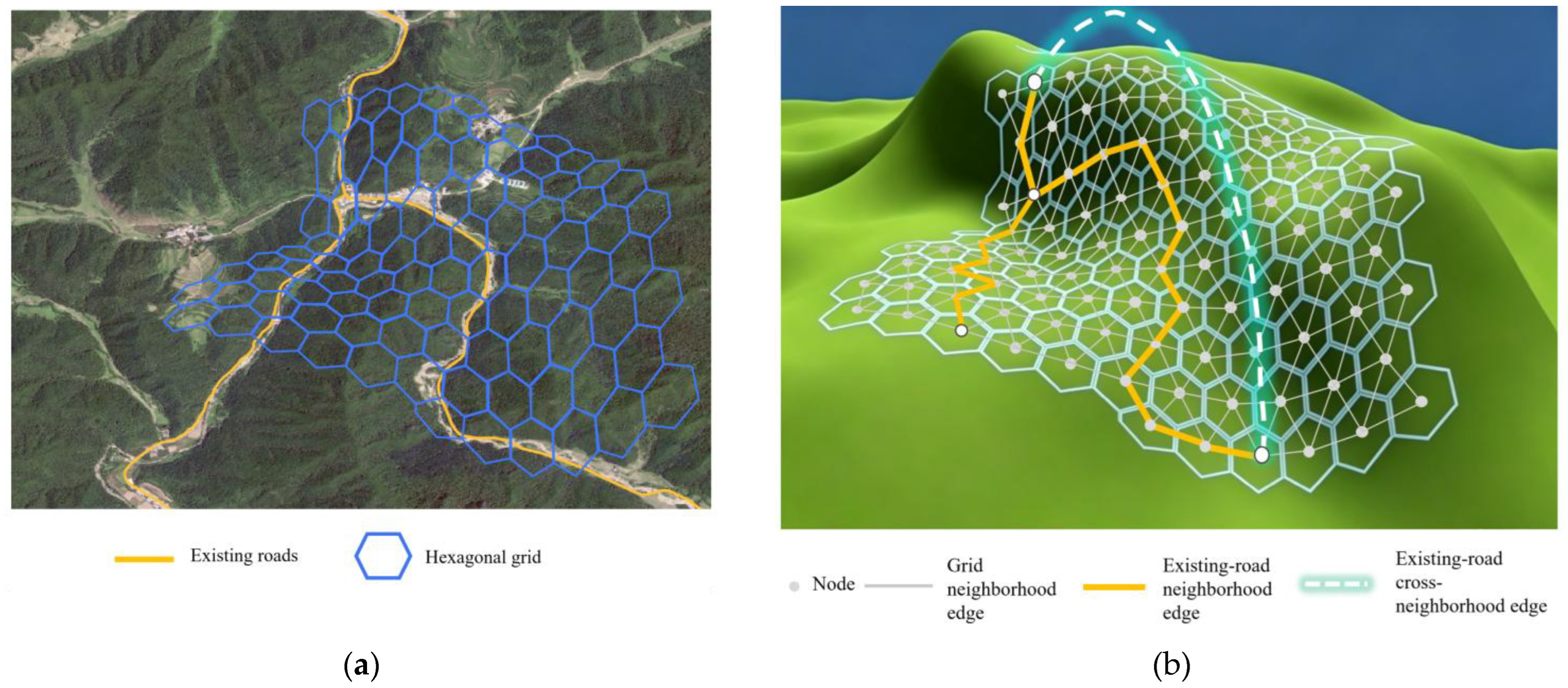
Figure 6.
Sequential road network generation under hierarchical constraints.
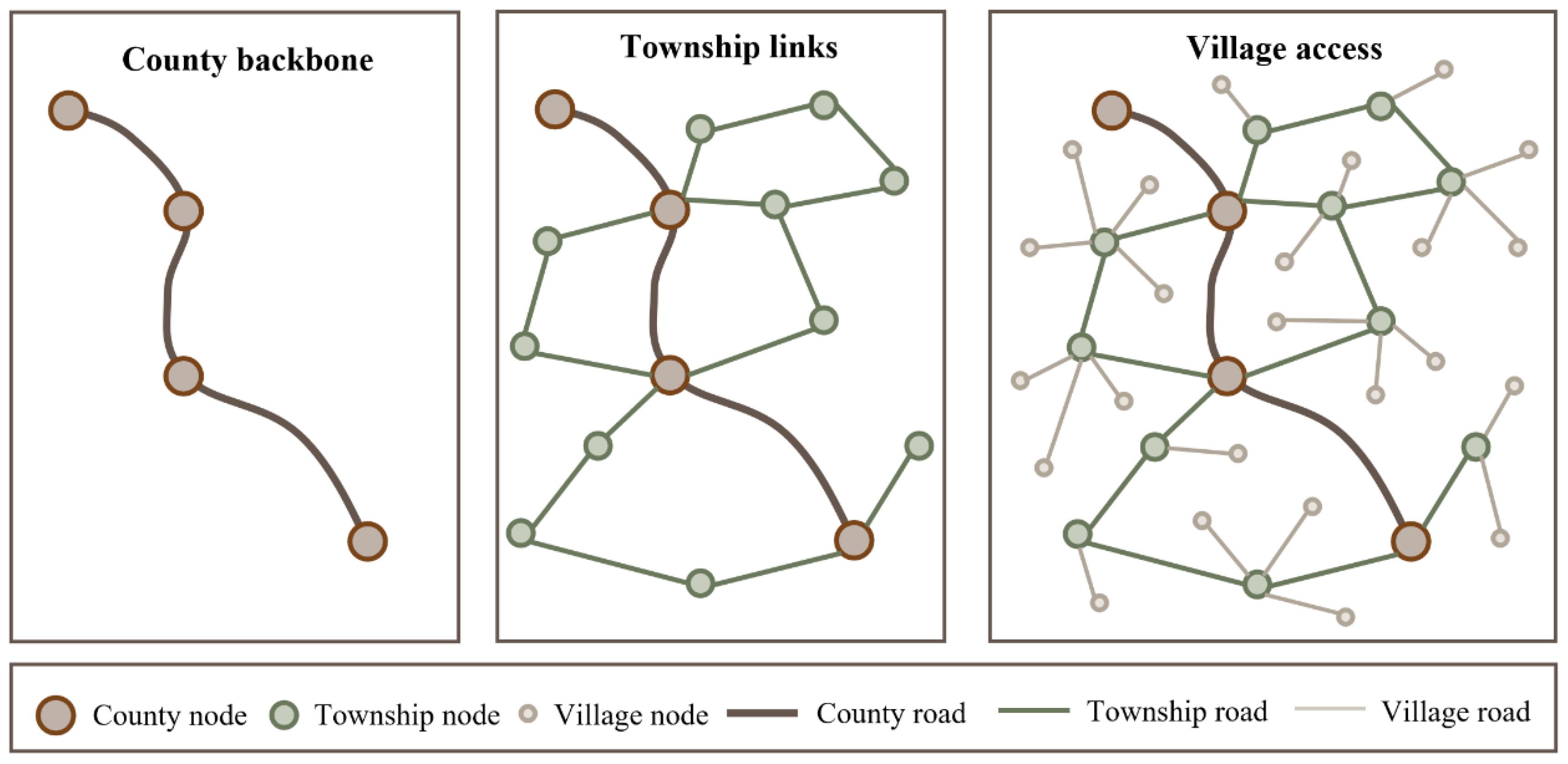
Figure 7.
Local network layouts generated by E1–E6.
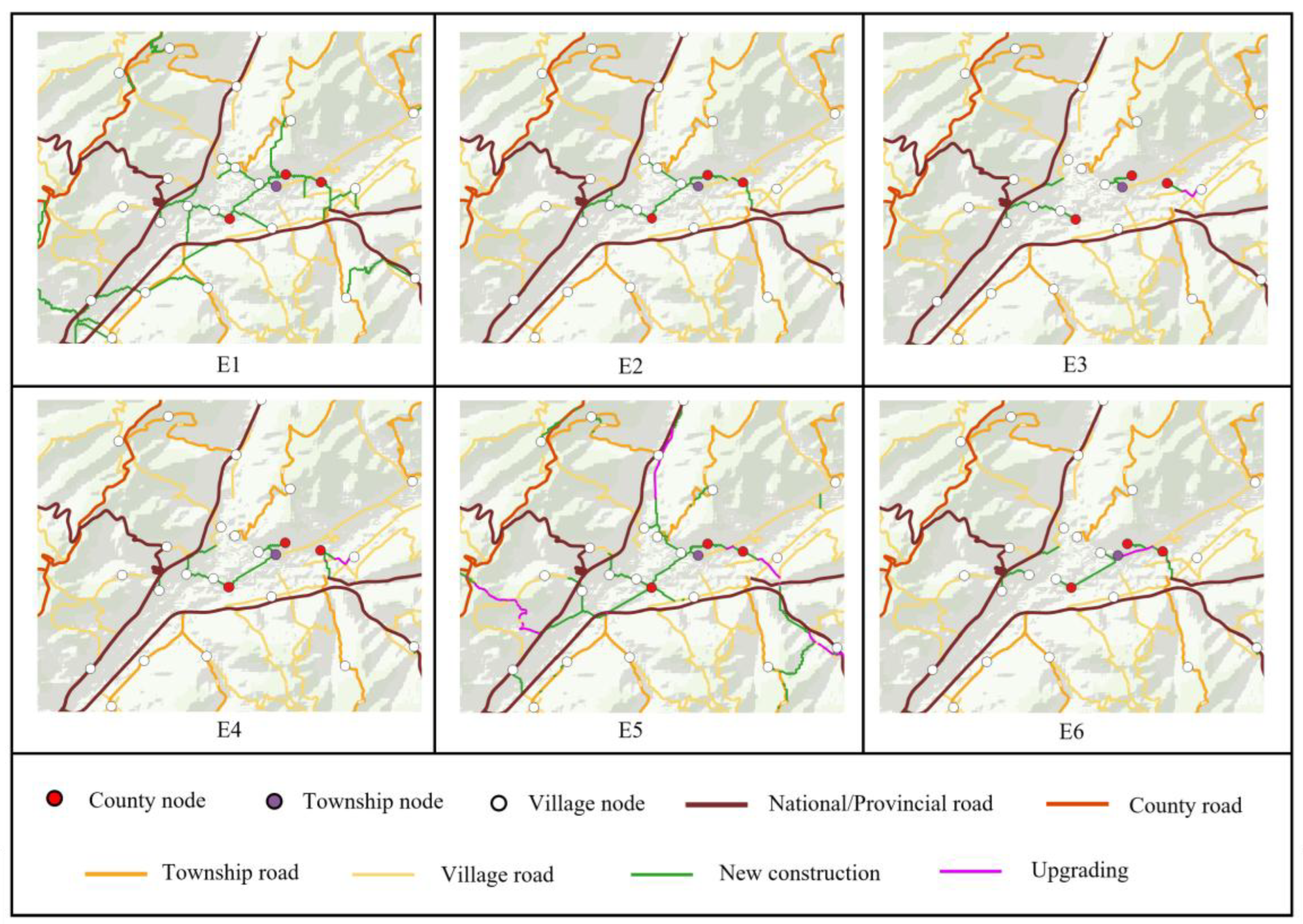

Table 1.
Input data and their main uses.
| Data | Main use |
| DEM | Elevation differences, three-dimensional distances, directional slopes, and terrain conditions |
| Administrative boundaries | Define the study area, node administrative affiliation, service groups, and township-specific village-road searches |
| Existing roads | Construct differentiated topological connections and identify roads available for reuse |
| Planning nodes | Administrative, transport (bus and railway stations and expressway entrances/exits), and economic nodes (industrial parks and tourist sites). Nodes are assigned to county, township, or village levels according to function, service coverage, and importance, supporting sequential backbone, linkage, and access generation. |
| No-build areas | Impassable areas, including water bodies, protected areas, and permanent basic farmland |
Table 1.
Hexagonal grid attributes and assignment methods.
| Category | Attribute | Assignment method | Main use |
| Geometric indexing | Cell ID, row, column, and center coordinates | Calculated from grid centers | Unique identification, spatial alignment, and six-neighbor lookup |
| Terrain | Center elevation | DEM sampling at each grid center | Elevation differences, three-dimensional distances, and slopes of neighboring edges and road segments |
| Administrative affiliation | County and township | Point-in-polygon matching of grid centers and administrative boundaries | Restrict search extents and organize planning nodes and village-road groups |
| Adjacency | Six neighboring nodes and edges | Generate six directions using row/column indices and odd/even column offsets | Construct the basic traversable graph |
Table 2.
Components and connection rules of the integrated graph.
| Symbol | Spatial entity | Generation or connection rule |
| VH | Nodes | Centers of valid hexagonal cells |
| EH | Grid neighborhood edges | Connect adjacent grid-center nodes |
| EA | Existing-road neighborhood edges | Road segments between consecutive access locations |
| ER | Existing-road cross-neighborhood edges | Connect permitted access points along actual road alignments |
Table 3.
Edge attributes of the integrated graph.
| Category | Field | Applicable edges | Meaning and assignment |
| Identifier | Edge ID | All | Primary key identifying each edge |
| Topology | Source ID | All | ID of the starting node |
| Topology | Target ID | All | ID of the ending node |
| Edge type | Type code | All | Grid neighborhood, existing-road neighborhood, or existing-road cross-neighborhood |
| Geometry | Edge geometry | All | Geometry of the grid or existing-road connection |
| Terrain | Source elevation | All | Extracted from the DEM |
| Terrain | Target elevation | All | Extracted from the DEM |
| Terrain | Slope angle | All | Check slope conditions and calculate costs |
| Road attributes | Road ID | Both existing-road types | Links to the source road feature; null for grid neighborhood edges |
| Road attributes | Road administrative category | Both existing-road types | Expressway, national, provincial, county, township, or village road |
| Road attributes | Technical class | Both existing-road types | Technical class of the existing road |
| Road attributes | Pavement type | Both existing-road types | Pavement type code |
| Search cost | Cost | All | Grid neighborhood costs calculated using the cost function |
Table 4.
Evaluation indicators, scoring rules, and weights.
| Indicator | Definition and scoring | Calculation and parameters | Weight (%) |
| Network composition | Shorter total network length and a larger existing-road share receive higher scores. The two normalized scores are averaged with equal weights. | Network composition score: zL: normalized length score (lower is better). zU: normalized existing-road share (higher is better). Lphysical: final network length; Uroad: existing-road share. Lphysical = Lroad + Lnew Lroad: length of existing roads used. Lnew: new-construction length represented by grid neighborhood edges. |
35 |
| Service accessibility | Time improvements are calculated for village–township government, township government–county seat, and village–county seat OD pairs. Their normalized scores are averaged equally; higher improvements are better. | Service accessibility score: : normalized improvement score. ηs: relative travel-time improvement. : pre-planning mean shortest time for service type s. : post-planning mean shortest time for service type s. |
35 |
|
Hierarchical compliance |
County-level continuity, township access to the county backbone, village access to its assigned township backbone, and connection errors. Reported separately without a scoring weight. |
County, township, and village compliance rates C1,C2,C3: : total county-level nodes and county-level nodes in the largest county-level connected component. : total township-level nodes and those connected to the county-level backbone. : total village-level nodes and those correctly connected to their assigned township backbone. |
|
| Construction requirements | Coefficients of 0, ρu and 1.0 are used for reuse, upgrading, and new construction. Lower construction requirements receive higher scores from 0 to 100. | Construction requirements score: Ibuild: construction requirements index. Lupgrade,Lnew: upgrading and new-construction lengths. |
30 |
| Composite score | Weighted sum of network composition, service accessibility, and construction requirements, with weights of 35%, 35%, and 30%. |
S = 0.35Zline + 0.35Zservice +0.30Zbuild |
100 |
Table 5.
Existing-road representation strategies.
| Code | Strategy | Treatment of existing roads |
| R1 | Uniform cross-neighborhood representation | All existing roads are represented by cross-neighborhood edges between endpoints, connected intersections, and attribute-change locations. |
| R2 | Category-specific combined representation | Expressways use cross-neighborhood edges between endpoints and entrances/exits. National and provincial roads use continuous segments between endpoints, intersections, and attribute-change nodes. County, township, and village roads are matched to nodes along their alignments to form neighborhood edges. |
Table 6.
Network organization strategies.
| Code | Organization | Node connection task |
| H0 | Global MST | One MST over all planning nodes, without county–township–village differentiation |
| H1 | Global OTSP | One OTSP visiting order for all planning nodes, without hierarchical differentiation |
| H2 | Sequential hierarchical generation | County and township OTSPs; township-specific rooted MSTs for village nodes |
| H3 | Hierarchical MSTs | County MST, township rooted MSTs, and village rooted MSTs under the same hierarchical constraints as H2 |
Table 7.
Edge-cost settings.
| Code | Grid neighborhood edges | Existing-road edges |
| K0 | New-construction cost from Equation (5) | Neighborhood edges: , without distinguishing reuse and upgrading. Cross-neighborhood edges: cE = 0. |
| K1 | New-construction cost from Equation (5) | Neighborhood edges: zero for reuse and ρu times the corresponding new-construction cost for upgrading. Cross-neighborhood edges: cE = 0. |
Table 8.
Combinations of the six experimental scenarios.
| Scenario | Representation R | Organization H | Cost K | Comparison |
| E1 | R1 | H2 | K1 | Uniform cross-neighborhood representation |
| E2 | R2 | H2 | K1 | Proposed complete scenario |
| E3 | R2 | H0 | K1 | Global tree organization |
| E4 | R2 | H1 | K1 | Global visiting-path organization |
| E5 | R2 | H2 | K0 | Uniform existing-road cost, without reuse/upgrading differentiation |
| E6 | R2 | H3 | K1 | Hierarchical tree organization under the same constraints |
Table 9.
Network composition by scenario.
| Scenario | Total network length (km) | Existing-road length used (km) | New-construction length (km) | Existing-road share (%) |
| E1 | 993.151 | 658.291 | 334.860 | 66.28 |
| E2 | 880.001 | 831.873 | 48.128 | 94.53 |
| E3 | 806.367 | 765.238 | 41.130 | 94.90 |
| E4 | 918.985 | 868.543 | 50.443 | 94.51 |
| E5 | 525.078 | 262.477 | 262.601 | 49.99 |
| E6 | 864.524 | 818.178 | 46.346 | 94.64 |
Table 10.
Mean shortest travel times and improvements in service accessibility.
| Scenario | Village–township government | Township government–county seat | Village–county seat | |||
| Time (min) | Improvement (%) | Time (min) | Improvement (%) | Time (min) | Improvement (%) | |
| Pre-planning | 13.794 | — | 39.359 | — | 40.742 | — |
| E1 | 8.889 | 35.56 | 24.071 | 38.84 | 26.946 | 33.86 |
| E2 | 11.635 | 15.65 | 24.463 | 37.85 | 29.372 | 27.91 |
| E3 | 15.188 | -10.10 | 30.104 | 23.51 | 32.381 | 20.52 |
| E4 | 11.977 | 13.17 | 24.750 | 37.12 | 29.433 | 27.76 |
| E5 | 8.321 | 39.68 | 22.994 | 41.58 | 25.645 | 37.06 |
| E6 | 12.454 | 9.72 | 37.608 | 4.45 | 42.505 | -4.33 |
Table 11.
Hierarchical compliance and connection errors.
| Scenario | County continuity (%) | Township access compliance (%) | Village-to-assigned-township compliance (%) | Isolated nodes | Prohibited interlevel connections | Cross-township connections |
| E1 | 100.00 | 100.00 | 100.00 | 0 | 0 | 0 |
| E2 | 100.00 | 100.00 | 100.00 | 0 | 0 | 0 |
| E3 | 28.57 | 5.26 | 100.00 | 0 | 5 | 0 |
| E4 | 28.57 | 36.84 | 100.00 | 0 | 8 | 0 |
| E5 | 100.00 | 100.00 | 100.00 | 0 | 0 | 0 |
| E6 | 100.00 | 100.00 | 100.00 | 0 | 0 | 0 |
Table 12.
Road lengths by construction type for E1–E6.
| Scenario | Reuse (km) | Upgrading (km) | New construction (km) | Total network length (km) | Construction requirements index |
| E1 | 658.291 | 0 | 334.860 | 993.151 | 0.3372 |
| E2 | 825.141 | 6.732 | 48.128 | 880.001 | 0.0593 |
| E3 | 764.417 | 0.821 | 41.130 | 806.367 | 0.0516 |
| E4 | 865.873 | 2.670 | 50.443 | 918.985 | 0.0566 |
| E5 | 231.716 | 30.761 | 262.601 | 525.078 | 0.5353 |
| E6 | 810.560 | 7.618 | 46.346 | 864.524 | 0.0589 |
Table 13.
Composite evaluation results.
| Scenario | Network composition | Service accessibility | Construction requirements | Hierarchical compliance | Composite score | Rank |
| E2 | 61.67 | 73.19 | 98.41 | Satisfied | 76.72 | 1 |
| E4 | 57.49 | 70.76 | 98.97 | Not satisfied | 74.58 | 2 |
| E3 | 69.95 | 37.13 | 100.00 | Not satisfied | 67.48 | 3 |
| E6 | 63.45 | 13.27 | 98.49 | Satisfied | 56.40 | 4 |
| E5 | 50.00 | 100.00 | 0.00 | Satisfied | 52.50 | 5 |
| E1 | 18.14 | 92.21 | 40.96 | Satisfied | 50.91 | 6 |
Table 14.
Sensitivity to the upgrading cost coefficient.
| Upgrading coefficient ρu | E2 total length (km) | E2 existing-road share (%) | E2 rank within setting |
| 0.4 | 851.298 | 96.02 | 1 |
| 0.6 | 880.001 | 94.53 | 1 |
| 0.8 | 873.107 | 92.58 | 1 |
Disclaimer/Publisher’s Note: The statements, opinions and data contained in all publications are solely those of the individual author(s) and contributor(s) and not of MDPI and/or the editor(s). MDPI and/or the editor(s) disclaim responsibility for any injury to people or property resulting from any ideas, methods, instructions or products referred to in the content. |
© 2026 by the authors. Licensee MDPI, Basel, Switzerland. This article is an open access article distributed under the terms and conditions of the Creative Commons Attribution (CC BY) license (http://creativecommons.org/licenses/by/4.0/).
Copyright: This open access article is published under a Creative Commons CC BY 4.0 license, which permit the free download, distribution, and reuse, provided that the author and preprint are cited in any reuse.