

Submitted:
07 October 2026
Posted:
14 October 2026
You are already at the latest version
Abstract
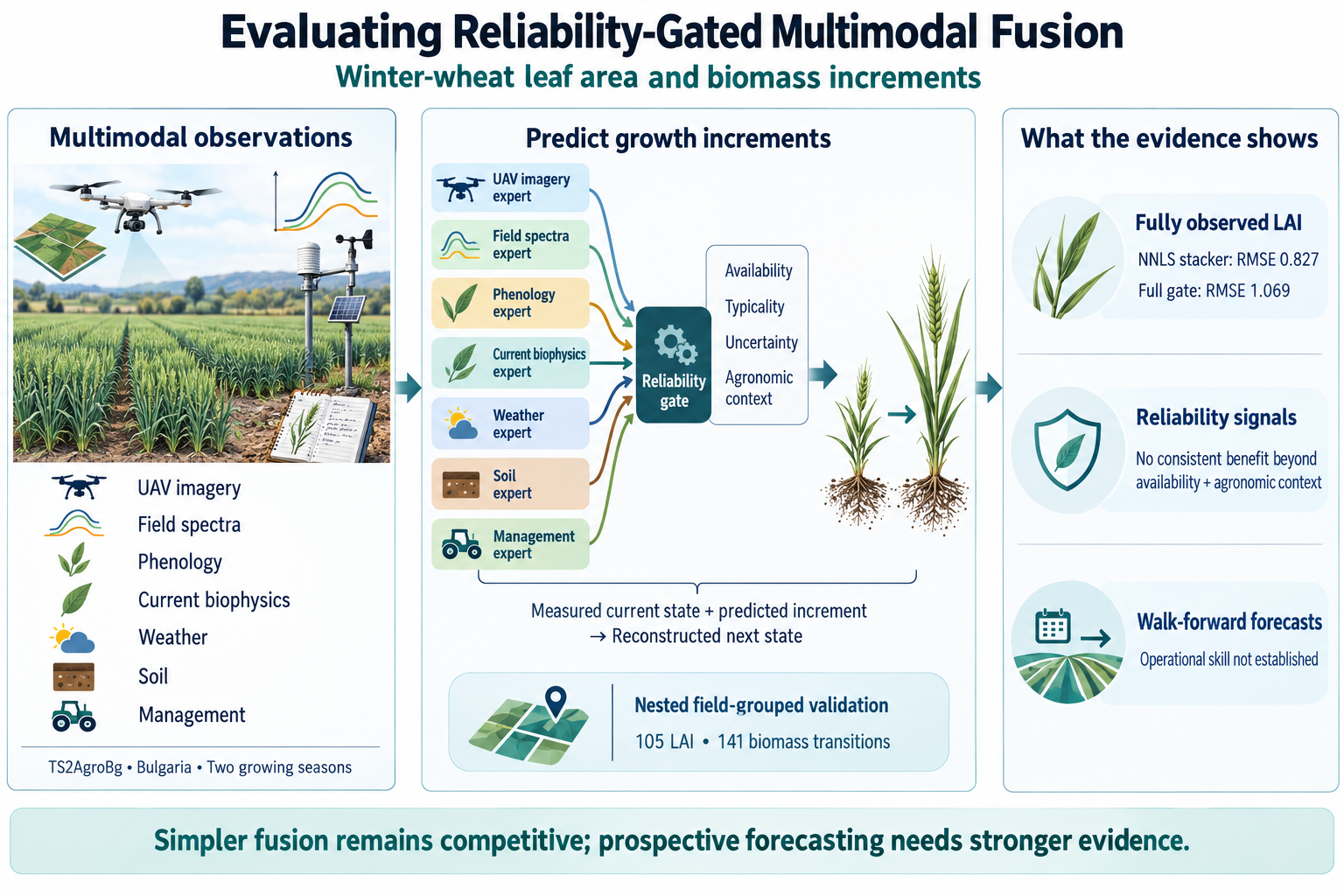
We evaluate whether typicality and uncertainty improve multimodal fusion of winter- wheat leaf area index(LAI)and biomass increments beyond availability-only gating(availability plus agronomic context). Consecutive elementary sampling unit (ESU) visits are kept when their 20m windows overlap (n = 105 LAI, n = 141 biomass); overlap is not a repeated plot. Nested field-grouped cross-validation does not favour the full gate. A nonnegative stacker is more accurate on fully observed ∆LAI (RMSE 0.827 vs 1.069). Availability-only gating has a slightly lower observed RMSE on fully observed biomass increments (101.1 versus 102.4), with no statistically significant difference detected (field Wilcoxon p = 0.23). No consistent field-level benefit of typicality and uncertainty was established. Withholding the current-biophysics expert from the increment predictor measured yt is still used in reconstruction—gives reliability-gated fusion (SARG) the lowest pooled biomass RMSE, but not a paired win versus availability-only (p = 0.42). Concatenated walk-forward does not establish usable next-campaign skill: ridge has a small numerical ∆LAI RMSE gain over the mean-increment baseline (2.190 vs 2.234), and every concatenated R2 remains negative. Reconstruction \(\widehat{y}_{t+1} = y_t + \widehat{\Delta y}\) uses the measured current state.
Keywords:
multimodal data fusion
; dynamic gating
; UAV multispectral imagery
; winter wheat
; growth-increment forecasting
; missing-modality robustness
; nested cross-validation
Introduction
Precision agriculture is not short of sensors. A drone returns Green, Red, Red-Edge and Near-Infrared reflectance at centimetre resolution; a ceptometer returns leaf area index (LAI) and absorbed radiation; a laboratory returns nitrogen concentration; a station streams temperature, radiation and soil moisture; a farm manager records variety, sowing density and predecessor crop. The difficulty is that these streams are informative at different times and in different amounts, and that fusion architectures rarely acknowledge it.
Consider the evidence that motivates this paper. On the spatially screened TS2AgroBg increments, unmanned aerial vehicle (UAV) patch statistics explain of LAI and a nonnegative stacker reaches , while the full gate is behind both (). For biomass, no statistically significant difference was detected between the gate and a ridge stacker (RMSE vs ; cluster-bootstrap RMSE CI to ). Availability-only gating is numerically ahead of the full reliability gate on fully observed biomass (RMSE vs ). Small pooled LAI improvements of the full gate over availability-only appeared in exploratory bootstrap analyses, but field-level Wilcoxon tests did not establish improvement across fields (unadjusted). A single global weight per modality—the ridge stacker of classical decision-level fusion (Wolpert 1992; Hall and Llinas 1997)— is required to average over campaign heterogeneity. It cannot express “trust the canopy image now, trust the phenological score in three weeks, and ignore the spectrum once the canopy has closed”.
We therefore replace the fixed combination rule with a gate. Writing for the prediction of the expert that sees modality only, the forecast is
where is the phenological (Zadoks) state at the time the forecast is issued, the forecast horizon, , and the availability, input typicality and predictive uncertainty of modality , and a learned intercept. The weights are produced by a small network, , so that the fusion mechanism itself is a function of crop development and sensor reliability rather than a constant of the dataset. The construction is a mixture of experts (Jacobs et al. 1991; Shazeer et al. 2017) that can also see agronomic context, in the spirit of dynamic and uncertainty-aware multimodal fusion (Xue and Marculescu 2023; Han et al. 2021). Phenology-aware multimodal models already exist. Liu et al. (2026) identify soybean stages with a dynamic gate; Huang et al. (2026) forecast strawberry yield from phenology-informed vision–weather series; Wang et al. (2026) estimate maize LAI with stacking and phenology-specific feature sensitivity. Increment-style growth forecasts are not new either: Senti et al. (2026) track winter-wheat LAI, including day-to-day . Once is measured, is just the increment written as a next state. Hierarchical and centralised or decentralised federation have already been tried for agricultural yield (Abouaomar et al. 2025; Mukherjee and Buyya 2025).
The research question is explicit: under what conditions, if any, do typicality and uncertainty improve fusion beyond availability alone? Availability-only gating still receives agronomic context (Table gate inputs): it is availability plus context, not availability in isolation. The gate may also see stage and horizon. We do not assume that the extra signals will help. The stress tests are withheld experts and increment forecasts that still need a measured . Negative results are retained: they are the evidence, not a prelude to a performance claim.
Two design choices run through the rest of the paper.
Forecast the increment, and do not readacross scales.
Dry above-ground biomass rises by almost two orders of magnitude between November and June, so on pooled campaigns. When the current state is observed and clipping in Equation reconstruct is inactive,
so the absolute and increment prediction errors are identical. Their values differ because the denominators and differ. A mean-increment baseline that predicts the training-set and then adds the measured therefore does not ignore the crop: it uses the current state and a constant growth step. It reaches on absolute next-campaign biomass and on the increment, which is what you expect when the target variance changes, not a split of skill into “seasonal progression”. We also report persistence () and a mean growth-rate baseline. We did not fit a calendar-only or stage-only predictor of , so we do not claim to have measured seasonal predictability beyond those controls.
Use the imagery.
Averaging a hyperspectral signature down to four band means is a stand-in for a drone, not a use of one. For every elementary sampling unit (ESU) we cut the matching window from the four-band orthomosaics and encode it. The fusion problem is then an image together with spectra, weather series and tabular records, not four extra columns.
We contribute:
A spatially screened increment , kept when consecutive windows overlap, and reconstructed as from the measured . Screening is not a check that the plot is the same. We also report a majority-overlap sensitivity.
A comparative evaluation of a reliability-conditioned mixture-of-experts (Equation gate intro) against availability-only gating, nonnegative stacking and nested expert-dropout under every withheld modality, asking when typicality and uncertainty help.
Nested field-grouped cross-fitting, field-bootstrap intervals, and exploratory unadjusted paired tests. No primary hypothesis was prespecified.
Related work and positioning
From fixed to dynamic fusion
The classical taxonomy separates fusion by abstraction level—data, feature and decision—and by uncertainty calculus (Hall and Llinas 1997; Khaleghi et al. 2013; Castanedo 2013; Baltrušaitis, Ahuja, and Morency 2019). Decision-level fusion trains a specialist per modality and combines the outputs by voting, stacking (Wolpert 1992) or Bayesian model averaging. Our nonnegative and ridge stackers come from that stacking literature. How well stacking survives a missing expert depends on the implementation—zeroing a weight is not the same as dropping a sample— which is why we test sensor loss rather than assume robustness. The usual limitation remains: the combination rule is fitted once for the whole dataset.
Adaptive mixtures of local experts (Jacobs et al. 1991) and their modern sparsely-gated descendants (Shazeer et al. 2017) instead learn an input-dependent gate. Dynamic multimodal fusion (Xue and Marculescu 2023) adapts computation per sample; trusted multi-view classification (Han et al. 2021) weights views by evidential uncertainty. Ma et al. (2021) learn from severely incomplete modalities with a missing-feature reconstruction network and Bayesian meta-learning. That is a reconstruction method. Reliability-gated fusion (SARG) does not fill in a withheld modality; it passes an availability vector ( is the finite-feature fraction), together with typicality and uncertainty, to the gate. Heteroscedastic heads (Kendall and Gal 2017) supply the per-expert uncertainty the gate can use. Stage, horizon and calendar features can also enter the gate. We try that option on TS2AgroBg; it does not improve accuracy.
Agricultural multimodal learning
Retrieval of LAI, APAR, cover fraction and biomass from Sentinel-2 and UAV multispectral imagery is mature (Verrelst et al. 2015), including on the Bulgarian winter-wheat campaigns that produced TS2AgroBg (Dimitrov et al. 2026, 2019; Roumenina et al. 2020). Deep multimodal fusion of UAV imagery with structural and thermal features has been shown to improve soybean yield prediction (Maimaitijiang et al. 2020). Multi-temporal UAV multispectral and digital vegetation indices have been used to predict rice grain yield (Zhou et al. 2017); that study does not use structural or thermal fusion. Convolutional models also operate directly on drone mosaics (Nevavuori, Narra, and Lipping 2019; Klompenburg, Kassahun, and Catal 2020). Phenology is now routinely an input or a target of multimodal models: Liu et al. (2026) fuse machine-learning and deep-learning pathways with a dynamic gate to identify soybean stages; Huang et al. (2026) couple visual phenology with weather embeddings for strawberry yield; Wang et al. (2026) report phenology-specific SHAP sensitivity in a stacked maize LAI estimator; and Senti et al. (2026) forecast winter-wheat LAI trajectories, including day-to-day increments, from satellite and meteorological time series. Phenology-aware fusion and increment-style growth forecasts are already in the literature. What we add is the reliability signals, the expert-withdrawal tests, and increment forecasts that use fewer ground-measured covariates—not a claim that we introduced phenology or increments.
Positioning
On the same Bulgarian landscape the usual retrieval question is “what is LAI now?”. We ask how much canopy will develop before the next campaign. Liu et al. (2026) predict soybean phenological stage; we treat phenology as an optional gate input, not as the thing to predict. Huang et al. (2026) forecast strawberry yield; we forecast a next-campaign LAI or biomass increment given the measured . Wang et al. (2026) estimate maize LAI now, with stacking and phenology-specific sensitivity; we forecast an increment and then drop sensors. Turning off agronomic context in the SARG gate does not reduce pooled increment skill on this sample. Against increment-style growth forecasts (Senti et al. 2026), the increment is a way to hold current state fixed, not what we claim to have invented; a growth-rate ablation then asks the harder per-day question. Cross-silo sharing in agri-food data (Durrant et al. 2022) and hierarchical or centralised/decentralised agricultural federation (Abouaomar et al. 2025; Mukherjee and Buyya 2025) are already discussed; Yang et al. (2019) survey federated learning in general. fed reports a neural optimisation run that standardises the concatenated training-client table in one place. That is not a field-local pipeline, we did not re-fit it after screening, and we do not treat it as a contribution.
Materials and Methods
Dataset: TS2AgroBg
We use the public TS2AgroBg dataset of Dimitrov et al.: georeferenced UAV multispectral imagery, ground spectra, crop biophysics and biochemistry, soil, phenology, management records and station weather from commercial winter wheat in Bulgaria (Dimitrov et al. 2026, 2025). It is released on Zenodo under CC BY 4.0. Figure ts2agrobg overview shows the source families and the keys that join them.
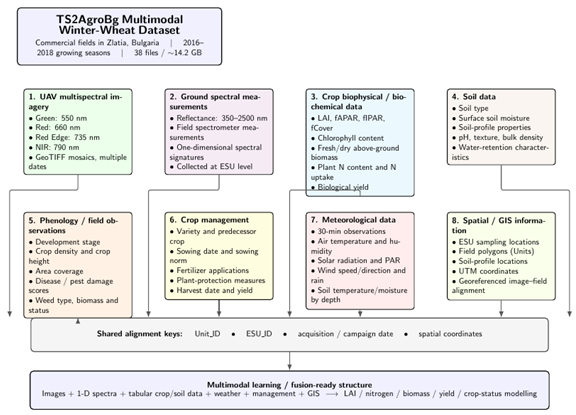
Overview of the TS2AgroBg dataset and its multimodal structure. The dataset combines unmanned aerial vehicle (UAV) multispectral imagery, ground spectral measurements, crop biophysical and biochemical variables, soil properties, phenological observations, crop-management records, meteorological measurements, and geospatial information. The modalities can be linked through common field identifiers, sampling-unit identifiers, acquisition dates, and geographic coordinates, enabling multimodal fusion for crop-status modelling.
TS2AgroBg covers two growing seasons (2016/17 and 2017/18) on commercial winter wheat of the Zlatia test site, collected under ESA PECS contract 4000117474/16/NL/NDe. Elementary Sampling Units are plots surveyed in six agricultural units. Campaigns are November 2016, March, April, May and June 2017, plus November 2017 and April 2018, giving 206 ESU visits over 60 spatially recurring plots. Phenological stages follow the decimal code of Zadoks, Chang, and Konzak (1974) and soil types follow WRB (IUSS Working Group WRB 2015).
Six agricultural units, twelve season–unit clients.
The dataset labels six commercial units per season. Those labels are not the same physical fields reused in 2017/18. Winter wheat is rotated, and the unit numbers are reassigned: and occupy different cadastral parcels (Figure client map, Table clients). The nearest same-label pair is and at ; U1 is apart across seasons, and units 4–6 of 2017/18 lie more than north of their 2016/17 namesakes. No cross-season client pair is closer than . The twelve season–unit identifiers are therefore twelve distinct places, and holding one out of training never leaks the same physical field from the other season. Within a season the units of a farm cluster can be as close as –; grouped cross-validation still holds the entire unit out. The grouping key is this season–unit identifier, matching the data-governance boundary of a farm operator in a given year.
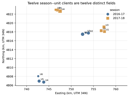
Centroid of each season–unit client in UTM 34N. Marker size is the number of ESU plots. Units 1–6 in 2016/17 and units 1–6 in 2017/18 are different commercial fields; the shared integer is a seasonal label, not a persistent parcel identifier.
Season–unit clients. Coordinates are mean ESU easting and northing (UTM 34N). Distance is to the nearest other client.
| Client | Season | Unit | Plots | Visits | Easting (m) | Northing (m) | Dist. (m) |
| S16-17_U1 | 2016/17 | 1 | 7 | 35 | 752 572 | 4 817 469 | 121 |
| S16-17_U2 | 2016/17 | 2 | 6 | 30 | 753 874 | 4 817 740 | 145 |
| S16-17_U3 | 2016/17 | 3 | 2 | 10 | 753 275 | 4 817 791 | 121 |
| S16-17_U4 | 2016/17 | 4 | 6 | 29 | 743 851 | 4 806 706 | 228 |
| S16-17_U5 | 2016/17 | 5 | 6 | 30 | 742 819 | 4 806 929 | 228 |
| S16-17_U6 | 2016/17 | 6 | 3 | 12 | 742 618 | 4 808 030 | 340 |
| S17-18_U1 | 2017/18 | 1 | 5 | 10 | 757 480 | 4 818 074 | 106 |
| S17-18_U2 | 2017/18 | 2 | 5 | 10 | 756 748 | 4 818 263 | 106 |
| S17-18_U3 | 2017/18 | 3 | 5 | 10 | 757 367 | 4 819 098 | 533 |
| S17-18_U4 | 2017/18 | 4 | 7 | 14 | 747 511 | 4 822 664 | 185 |
| S17-18_U5 | 2017/18 | 5 | 5 | 10 | 746 893 | 4 822 915 | 90 |
| S17-18_U6 | 2017/18 | 6 | 3 | 6 | 746 536 | 4 822 968 | 90 |
UAV Patch Extraction
The public release ships the imagery as seventeen archives (one per season, unit group and flight date), each holding four single-band reflectance GeoTIFFs—Green, Red, Red Edge and Near-Infrared—at ground sampling distance in EPSG:32634, totalling approximately . Rather than unpacking them, the rasters are read in place through the GDAL zip layer and only the ESU windows are materialised. For each visit the square centred on the recorded ESU centroid is read as a native window per band, the sensor no-data value and non-physical reflectances are masked, and the result is NaN-aware average-pooled to a tensor
retained only when at least of the pixels are valid in all four bands. This yields 161 of 206 ESU visits with imagery. The 45 missing cases are genuine acquisition gaps rather than processing failures: there was no June 2017 flight, and units 1–3 were not flown in November 2017. Missing UAV is not a nuisance: it is one of the availability conditions the gate is meant to handle.
Figure uav patches shows extracted patches. The phenological progression is unmistakable—mottled, partly bare soil in November (patch-mean ) closing to a dense uniform canopy in April ()—and sprayer tramlines are resolved as dark lines, which confirms both the georeferencing and the presence of real sub-plot texture.
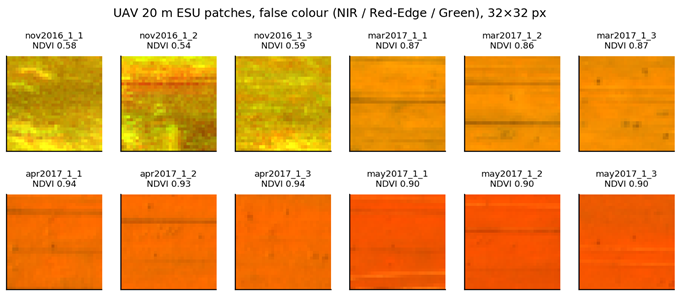
ExtractedUAV patches for ESUs of unit 1 across four campaigns, shown as false colour (NIR / Red-Edge / Green) at theresolution used by the image encoder. Canopy closure between November and April is visible, as are sprayer tramlines within the plot.
Each patch contributes two representations. The first is a set of 31 patch-level statistics: per-band mean, standard deviation and 10th/90th percentiles; the means and standard deviations of NDVI, NDRE, GNDVI, CIRE and SAVI computed pixel-wise; the within-patch NDVI coefficient of variation, inter-percentile range and mean gradient magnitude as measures of canopy patchiness; and the valid-pixel fraction, which doubles as the UAV term in the typicality score . The second is the raw tensor, consumed by the convolutional encoder of Section encoders. Reporting both is deliberate: they turn out to behave very differently at this sample size (Section res methods).
Unification of the Remaining Modalities
The remaining streams have to be joined on plot and date before they are features. Each ESU identifier is parsed into a stable plot key (season, unit, ESU) and modalities are joined on that key and campaign date. The spectral modality integrates ASD FieldSpec reflectance over Sequoia/Sentinel-2 analogue windows (Green 540–570 nm, Red 640–680 nm, Red-Edge 710–740 nm, NIR 770–810 nm), optical bins from 400–1000 nm, and the indices NDVI, NDRE, GNDVI, EVI2, SAVI, CIRE, SR, MTCI and NDWI. Phenology contributes density, height, visually assessed cover, damage and weediness scores, a mid-range Zadoks stage and days after sowing. Biophysics contributes LAI (measured in situ; estimation errors and sampling are reviewed by Weiss et al. (2004)), IPAR, APAR, Cover, chlorophyll, fresh and dry biomass and nitrogen concentration and uptake, always of the observation campaign and never of the target campaign. Soil contributes campaign ESU gravimetric moisture and nearest-profile topsoil clay, organic carbon, pH and bulk density from campaign pits (Dimitrov et al. 2026, 2025), not a public soil map. Weather is summarised from two on-site meteorological stations (half-hourly records into 7- and 30-day windows plus growing degree-days since sowing), not a reanalysis or GIS weather layer. Station coverage is incomplete: every November 2016 visit lacks the 7-day meteorological window, and half of the April 2017 visits do. Empty weather features are median-imputed inside each training fold only. Neighbouring agricultural units lie – apart within a season (Table clients); grouped cross-validation holds a unit out but cannot remove spatial dependence among remaining neighbours, which limits claims of geographic generalisation. Management contributes sowing density, field area, variety and predecessor codes and campaign index. The forecast gap is not an input to the management expert—it would let that expert infer how much growth time remains—and is supplied only to the gate as context. Median imputation is fitted inside each training fold only, with empty features preserved so that an absent modality never silently drops a sample.
Spatial screening of.
The increment mixes locations if consecutive visits do not sample the same ground. The published column dictionary states that an ESU is a plot whose centre is Point_X_UTM34/Point_Y_UTM34 (WGS84 / UTM 34N). UAV patches use the same square. Two axis-aligned windows share some ground if and only if and , equivalently overlap fraction . That any-overlap screen is plot geometry, not an RMSE-tuned cutoff. It removes large identifier discontinuities; it does not establish that both measurements represent the same sampling area. A sliver of shared ground ( occurs among retained pairs) is still two mostly distinct plots. Table spatial reports displacement and overlap-fraction quantiles among pairs that pass the any-overlap screen. Median displacement is (LAI) and (dry above-ground biomass, AGBd); the 90th percentiles are and . Median overlap fraction is (LAI) and (biomass). Fourteen LAI and seventeen biomass pairs that overlap at all have .
A stricter, independently justified rule requires majority shared area, : more than half of the window is common ground. That is still geometry, not a threshold chosen because it improves RMSE. It leaves LAI and biomass transitions (Table majority; run v20260920_majority_overlap). That sensitivity repeats fully observed fusion and missing-modality comparisons; it does not repeat walk-forward. The main fully observed and gate-versus-availability findings hold: the full gate is not the most accurate fully observed model (nested dropout on LAI; no-reliability on AGBd); availability-only remains numerically ahead of or comparable to the full gate (LAI vs , ; biomass vs , ); under biomass biophysics withdrawal SARG still has the lowest pooled RMSE ( vs availability-only , nested dropout , masked ridge , nonnegative least squares (NNLS) ; vs availability ). Two rankings change: nested dropout overtakes NNLS on fully observed LAI, and availability-only is numerically ahead of SARG under LAI biophysics withdrawal ( vs ). The campaign documentation does not describe relocating an ESU between visits. Five November 2016March 2017 jumps of – fail even any-overlap ( LAI, biomass) and are identifier discontinuities relative to sibling-ESU medians (–). Tree-expert fusion, missing-modality and walk-forward tables use the any-overlap screened sample ( / ); majority-overlap did not repeat walk-forward. Neural federation and the reduced-input ladder were not re-fit after screening (hist / fed). Pair manifests are in the Zenodo reproducibility deposit (Bakır and Salman 2026).
Growth-Increment Targets
Let be the unified vector of plot at campaign . For a state variable the primary target is the increment to the next campaign,
and the absolute forecast is recovered by
Equation [eq:reconstruct] is not a remote-state estimator: is the measured current LAI or biomass. Historical reduced-input rungs in hist change which covariates enter , not whether is observed. Transitions are NovMar, MarApr, AprMay and MayJun in 2016/17 and NovApr in 2017/18. After excluding pairs whose windows do not overlap, LAI and biomass increments remain on the any-overlap screen ( / under majority overlap).
Consecutive-visit spatial audit. Any-overlap:. Majority:(more than half thewindow shared). Quantiles are among any-overlap pairs. Displacement in metres;is unitless overlap fraction.
| Pairs | Any-overlap | Majority | Disp. | Disp. | min | |||
| LAI | 108 | 105 | 91 | 3.84 | 9.39 | 0.75 | 0.09 | 14 |
| AGBd | 146 | 141 | 124 | 2.86 | 9.34 | 0.82 | 0.05 | 17 |
Majority-overlap sensitivity (; more than half thewindow shared). Nested field-grouped cross-fitting on v20260920_majority_overlap. Fully observed models and biophysics-withdrawal comparators; walk-forward was not repeated. Best fully observed RMSE in each column in bold. This rule is geometry, not RMSE-tuned.
| LAI () | AGBd () | |||
| 2-3(lr)4-5 Method | RMSE | RMSE | ||
| NNLS stacker | 0.854 | 0.743 | 115.1 | 0.831 |
| Dropout nested | 0.839 | 0.752 | 123.9 | 0.805 |
| Ridge stacker | 0.928 | 0.697 | 112.5 | 0.839 |
| SARG availability only | 0.934 | 0.693 | 98.7 | 0.876 |
| SARG no reliability | 0.949 | 0.683 | 98.3 | 0.877 |
| SARG full | 1.001 | 0.647 | 101.6 | 0.869 |
| Biophysics withheld, SARG | 1.049 | 0.612 | 107.3 | 0.853 |
| Biophysics withheld, avail. only | 0.958 | 0.677 | 111.1 | 0.843 |
| Biophysics withheld, dropout nested | 0.963 | 0.674 | 129.3 | 0.787 |
| Biophysics withheld, ridge masked | 1.010 | 0.641 | 180.5 | 0.586 |
| Biophysics withheld, NNLS masked | 1.134 | 0.547 | 246.1 | 0.229 |
Because campaign gaps are unequal—NovemberMarch is months, AprilMay is weeks—the increment still contains a horizon-length effect. We therefore also report a growth-rate ablation
where is known at forecast time. Predicting asks how rapidly the crop is developing rather than how much it will change over an interval of known length. It does not replace the increment task.
The default accuracy protocol is field-out GroupKFold over the twelve season–unit clients of Table clients: no physical field contributes training and test rows in the same fold. Walk-forward and cold-start splits (Section res wf) are a different protocol and are labelled as such; they are not field-grouped cross-validation. Unless noted, results use random seed 42. Point estimates of RMSE and from field-out folds are accompanied by percentile intervals from a field-level (cluster) bootstrap (Field and Welsh 2007). Methods are compared paired on the same held-out fields, , with a Wilcoxon signed-rank test on the field-level differences. Those tests are exploratory: no primary missing-modality hypothesis was prespecified, and -values are unadjusted for the number of modalities and targets. Ordinary row bootstrap is not used: rows inside a field share soil, cultivar and management and are not independent (Roberts et al. 2017).
Reliability-Gated Multimodal Fusion
Figure architecture is the evaluated tree-expert protocol. Each ExtraTrees encoder returns a prediction and an uncertainty; the UAV branch uses 31 patch statistics, not a CNN. The gate turns reliability signals—and, if we switch it on, agronomic context—into convex weights; the weighted sum plus a learned intercept is an increment, added to the measured current state. A compact CNN on the UAV patch is a neural alternative that was not re-fit after screening. A federated optimisation run with centralised preprocessing is summarised in fed and reported in the Zenodo deposit (Bakır and Salman 2026); it is not part of the main protocol.
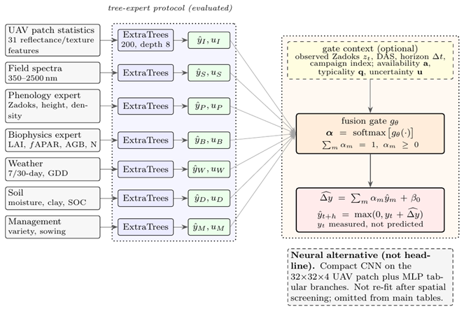
Tree-expert reliability-gated fusion used in the main tables. Each ExtraTrees expert (200 trees, depth 8) consumes one modality—UAV as 31 patch statistics, not a CNN—and returns a predictionand an uncertainty. The gatemaps reliability signals and, optionally, agronomic context (observed Zadoks, days after sowing, horizon, campaign index;is not an input to the management expert) to a convex weight vector. The forecast includes a learned interceptand is added to the measured current state. A compact CNN on theUAV patch is a neural alternative that was not re-fit after spatial screening and is not a headline result.
Modality Encoders and Experts
Seven modalities are encoded as in Equation encoders,
We use two encodings, because they suit different sample sizes.
Randomised-forest experts.
Each modality is given an extremely randomised trees regressor (Geurts, Ernst, and Wehenkel 2006) with 200 trees of depth 8 after fold-local median imputation and standardisation. The ensemble supplies both the prediction and its uncertainty: with trees producing ,
where is the median training spread of modality , so that is comparable across modalities. For this family the UAV modality enters as the 31 patch statistics of Section uav.
End-to-end neural experts.
The same seven modalities are alternatively encoded by a single network. The image branch is a compact CNN—three stride-2 convolutions with 12, 20 and 24 channels, batch normalisation, global average pooling and a linear projection to a 12-dimensional latent—applied to the raw patch; the six tabular branches are two-layer perceptrons into the same latent space. Each latent receives a heteroscedastic head (Kendall and Gal 2017) returning a mean and a log-variance,
so the uncertainty consumed by the gate is learned rather than derived from ensemble spread. Training minimises the fused squared error plus the mean per-expert Gaussian negative log-likelihood, which keeps the individual meaningful, using AdamW (Loshchilov and Hutter 2019). The network is trained in one place: an inner validation split and early stopping (patience ). It is not the federated trainer, and we did not re-fit it on the screened sample.
Reliability Signals
For every sample and modality the gate receives three scalars besides the prediction. Availability is the fraction of finite raw features in modality , which is for an ESU with no UAV coverage and for a complete record. Input typicality combines an in-distribution score with an explicit completeness term,
where is the training-standardised value of feature and is the valid-pixel fraction for the UAV modality, the spectrum-present indicator for the spectral modality, and otherwise. We call input typicality, not sensor quality: it measures how ordinary the feature vector looks to the fitted expert. Whether it tracks expert error is an empirical question, reported in Section res methods. Uncertainty is given by Equation tree unc or by the heteroscedastic head. It is consumed by the gate but is not independently validated against expert absolute error on this dataset: no grouped-inner Spearman table for versus error was saved, so that diagnostic is reported only for .
The agronomic context vector
The optional context vector supplied to the gate at forecast time comprises: Zadoks scaled by (or the thermal-time proxy when is absent); days after sowing; horizon ; campaign index; and ; the interaction ; and a one-hot encoding of Zadoks principal stage over . That vector is independent of the phenology expert. Withholding the phenology expert at inference replaces its prediction with the training-fold mean increment and sets , where is a fixed missing-expert sentinel inside the clip of Table gate config (Table withdrawal). On the scaled target used to train the gate, , that mean increment is zero; on the original increment scale it is not. The procedure does not blank observed Zadoks, days after sowing or campaign index from , so it is phenology-expert withdrawal, not complete loss of phenological information. The ablation labelled “no stage context” in hist sets use_context=False: it removes this entire vector, not only . Calendar, horizon and campaign features are then removed together with phenology. When ground phenology scoring is unavailable in the historical reduced-input configuration of hist, is replaced by the thermal-time proxy so the remaining context stays defined. Gate ablation switches are listed in Table gate inputs.
The gate is a one-hidden-layer network with a learned global preference and a learned temperature ,
and the forecast is , mapped to the absolute scale by Equation reconstruct. Two implementation details are essential.
- The gate is trained on out-of-fold expert predictions. If it saw in-sample predictions, every expert would look almost perfect and there would be nothing to learn. Meta-features are generated by a five-fold split within the training fold.
- That inner split is field-grouped, matching the outer protocol. A protocol diagnostic that compared inner-split policies on an earlier SARG implementation (before was removed from the management expert) found random-inner () versus grouped-inner () on LAI (Figure inner cv; (Cawley and Talbot 2010; Roberts et al. 2017)). That is not the gate in the main tables. After restricting to gate context, the historical unfiltered grouped-inner SARG was (). Primary fusion, missing-modality and walk-forward tables use the spatially screened run v20260920_spatial_verified (SARG LAI RMSE , ). Random inner folds are reported only as an optimistic sensitivity. The gate warm-start is not the NNLS comparator of Section setup. The comparator is unconstrained-sum nonnegative linear regression with an intercept (scikit-learn, nonnegative coefficients, intercept on). The warm-start instead solves intercept-free on the inner out-of-fold expert matrix , L1-normalises onto the simplex, and sets . Softmax of therefore starts at a fixed convex combination; is a separate learned intercept, initialised at zero. Weight decay is applied to the context trunk only, so and are not pulled toward uniform weights.
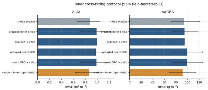
Inner-split protocol diagnostic on an earlier SARG implementation (management expert still saw). Random inner folds (orange) make that model look stronger than a ridge stacker onLAI; grouped inner folds do not. This figure is a protocol diagnostic on an earlier unfiltered implementation. Primary tables use v20260920_spatial_verified.
Centralised Tree-Expert Protocol
The main tables use ExtraTrees experts and a small gate (sarg). fed has a neural federated run that imputes and standardises the concatenated training-client table in one place. That is not field-local training, and we did not re-fit it after screening.
Training fold grouped by season–unit clients Field-grouped five-fold split of ; fit one ExtraTrees expert per modality on each inner complement; record out of fold. Warm-start from non-negative least squares of on those ; fit on the out-of-fold signals; refit experts on all of . Predict , then using measured .
Tree-expert SARG configuration used in Table param / Table methods / Table missing / Table wf simple (v20260920_spatial_verified). Inner out-of-fold preprocessing is fold-local: each inner complement fits its own median imputer and standardiser; raw tree-spread is then divided by the median out-of-fold spread of that modality on the outer training fold and clipped to. A withheld expert is not that clip: itsis the fixed sentinelin Table withdrawal. Deployed experts are refit on the full outer training fold with a new imputer/scaler; test-timeuses the same fold-level median.
| Item | Setting |
| Outer split | GroupKFold, 6 folds over 12 season–unit clients |
| Inner expert OOF | GroupKFold, 5 folds on outer-training clients |
| Gate width | one hidden layer, 16 tanh units; input |
| Experts | ExtraTrees, 200 trees, depth 8, min. leaf 2 |
| UAV encoding | 31 patch statistics (CNN alternative not re-fit) |
| Optimizer | AdamW; learning rate |
| Weight decay | on the context trunk only |
| Training duration | at most 1500 epochs; early stopping patience 200 |
| Model selection | hold out of training clients; restore best validation MSE |
| Target scaling | inside the gate; invert on output |
| Temperature | clamped to |
| Intercept | learned not part of the softmax |
| Warm-start | intercept-free NNLS, L1-normalised to the simplex, then |
| Entropy regulariser | off () |
| Seed | 42 |
Experimental Setup
All models share the unified table, the seed, and GroupKFold over the twelve season–unit clients unless a different protocol is named. Compared methods on the screened sample are: data-level (early) fusion with gradient-boosted trees (Chen and Guestrin 2016); a ridge stacker over the seven ExtraTrees experts; a nonnegative linear stacker (NNLS: unconstrained-sum nonnegative regression with an intercept); SARG; an availability-only gate; a no-reliability gate; and a ridge trained with expert-column dropout. Availability-only gating still receives ; it is availability plus agronomic context (Table gate inputs). NNLS masking zeros the dropped coefficient and keeps the intercept; remaining weights are not L1-renormalised. Ridge masking zeros and L1-renormalises. Dropout probability is selected in by inner GroupKFold on the training clients of each outer fold; every fold selected . Feature-level networks and the CNN branch were not re-fit after spatial screening. Seven single-modality ExtraTrees baselines use the same splits. A growth-rate ablation trains the same models on and maps back with Equation rate. That ablation, and absolute-trained counterparts, belong to the historical unfiltered sample; Figure agbd param shows learned fusion models that are increment-trained on the screened run, together with the baselines of Table param.
Gate ablations and expert-withdrawal encodings are defined in Table gate inputs / Table withdrawal. Unavailable experts do not receive exactly zero weight: softmax still assigns whatever mass produces from and . Stacker masking is different: NNLS zeros the dropped coefficient; ridge zeros and L1-renormalises.
Gate ablation inputs on the screened run. Agronomic contextincludes observed Zadoks, days after sowing, campaign index and horizon, and remains on for the availability-only and no-reliability gates. A disabled block is replaced by zeros, not removed from the network.
| Configuration | Context | Availability | Typicality | Uncertainty |
| Full gate (SARG) | yes | yes | yes | yes |
| Availability-only | yes (kept) | yes | zeroed | zeroed |
| No-reliability gate | yes | zeroed | zeroed | zeroed |
| No stage context (historical) | zeroed | yes | yes | yes |
Inference-time expert withdrawal versus reconstruction. Phenology-expert withdrawal removes the phenology expert only; observed Zadoks remains in gate context. It is not complete loss of phenological information. Biophysics-expert withdrawal removes LAI/APAR/AGB/N from the increment predictor; measuredis still required by Equation reconstruct.
| Quantity | Representation when withheld | Zero weight? |
| Expert prediction | training-fold mean increment | no; softmax may still assign mass |
| Availability | — | |
| Typicality | — | |
| Uncertainty | fixed sentinel (inside the clip; not the range maximum) | — |
| Phenology expert | as above; height, density, observed Zadoks dropped from that expert | observed Zadoks, DAS and campaign index remain in |
| Biophysics expert | as above; current LAI/APAR/AGB/N dropped from that expert | measured still added in Equation reconstruct |
Numbers in the abstract, Table param / Table methods / Table missing / Table wf simple and Section conclusions come only from the spatially screened run v20260920_spatial_verified ( LAI, biomass, any-overlap). The inner-split diagnostic (Figure inner cv) and the unfiltered historical analyses in hist / fed (gate weights, reduced-input ladder, CNN, federation) sit outside those claims.
Metrics are RMSE, MAE and , with field-bootstrap intervals and paired per-field Wilcoxon tests against the ridge stacker. Mean absolute percentage error is deliberately not reported for increment targets, because increments cross zero and the statistic diverges. Implementation is Python 3.13 with scikit-learn, XGBoost, PyTorch and rasterio on CPU; patch extraction over the seventeen flight archives takes about eleven minutes and is cached.
Results
Increments versus absolute future states
Table param reports increment-trained models scored on both scales: the implied absolute state is Equation reconstruct, not a separately trained absolute-state model.
Absolute next-campaign biomass can look almost solved ( for increment-trained SARG in Table param). That number is not increment skill. On pooled campaigns is much larger than , so the same residuals produce a higher absolute . A baseline that predicts the training-set mean increment and adds the measured already reaches on absolute biomass and on AGBd. Persistence and a mean growth-rate baseline are in Table param for both targets (biomass mean-rate RMSE , on AGBd). We did not train a calendar-only or stage-only model. On the increment scale, no statistically significant difference was detected between the gate and the ridge stacker (RMSE vs ; cluster-bootstrap RMSE CI to ). The median per-field is , which is about the size of the field-to-field spread on this sample—we do not call noise as a general rule.
Leaf area index really does move: persistence on the absolute scale. That is not proof there is no calendar shortcut; we never fitted a calendar-only model. The climatological increment has on LAI. The nonnegative stacker is the most accurate fusion model on fully observed LAI (RMSE , ), ahead of nested dropout (), early fusion (), the ridge stacker () and SARG ().
Increment-trained models on the spatially screened sample, scored on both scales. RMSE is identical across the two score columns whenis observed and clipping is inactive;differs because. Run v20260920_spatial_verified.
| Absolute | Increment | |||
| 2-3(lr)4-5 Method | RMSE | RMSE | ||
| Leaf area index, | ||||
| Persistence | 2.240 | 2.240 | ||
| Mean increment | 1.641 | 0.149 | 1.641 | |
| Mean rate | 2.227 | 2.227 | ||
| NNLS stacker | 0.827 | 0.784 | 0.827 | 0.744 |
| Dropout nested ( inner-selected) | 0.856 | 0.769 | 0.856 | 0.726 |
| Early fusion | 0.887 | 0.752 | 0.887 | 0.705 |
| Ridge stacker | 0.913 | 0.737 | 0.913 | 0.688 |
| SARG | 1.069 | 0.639 | 1.069 | 0.571 |
| Dry above-ground biomass (), | ||||
| Persistence | 421 | 0.260 | 421 | |
| Mean increment | 279 | 0.675 | 279 | |
| Mean rate | 869 | 869 | ||
| SARG no reliability | 101 | 0.957 | 101 | 0.868 |
| SARG availability only | 101 | 0.957 | 101 | 0.867 |
| SARG full | 102 | 0.956 | 102 | 0.864 |
| Early fusion | 104 | 0.955 | 104 | 0.860 |
| Ridge stacker | 105 | 0.954 | 105 | 0.857 |
| NNLS stacker | 110 | 0.950 | 110 | 0.843 |
| Dropout nested | 126 | 0.934 | 126 | 0.794 |
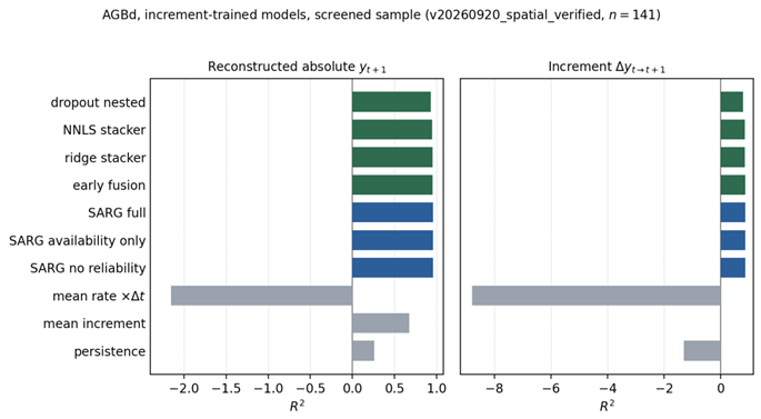
Dry above-ground biomass on the spatially screened sample (v20260920_spatial_verified,). All learned fusion models shown are increment-trained; baseline definitions follow Table param. Absolute-trained and growth-rate variants from the historical unfiltered sample are not shown.differs because. The mean-increment baseline adds the training-setto measured; it is not a calendar-only model and does not ignore the crop.
Fusion Strategies and Gate Ablations
Table methods compares fusion strategies on the increment, still under nested field-grouped cross-fitting on the screened sample. The full gate is not the most accurate fully observed model. On LAI, UAV patch statistics remain the strongest single modality (); the nonnegative stacker reaches , nested dropout , the ridge stacker , and SARG . On AGBd, no statistically significant difference was detected between SARG and the ridge stacker (RMSE vs ; cluster-bootstrap RMSE CI to ; median per-field ). Availability-only (availability plus agronomic context) and no-reliability gates are slightly better than the full gate on fully observed biomass (RMSE and vs ; Wilcoxon vs availability-only). Forecasting the absolute next state is a fair task if one says so; a higher absolute is still not increment skill.
No consistent benefit beyond availability was established.
Dropping typicality and uncertainty, or dropping all reliability inputs, does not hurt fully observed accuracy (LAI ; biomass ). The comparison that tests the reliability claim is the full gate versus availability-only gating (availability plus agronomic context) (Table avail), not versus a fixed stacker. Field Wilcoxon tests and cluster-bootstrap intervals of pooled RMSE answer different questions and need not agree. None of the field Wilcoxon tests reach unadjusted . The LAI bootstrap intervals exclude zero at the fourth decimal place, a difference of about RMSE, while the field tests do not ( and ). Those tests are exploratory and unadjusted; a nonsignificant field test is not equivalence. Row-wise Spearman tests of against expert error ignore the fact that rows share a field. On biomass, soil and weather look convincing at row level () and disappear once each field is one observation ( and ). UAV typicality does not track error. enters the gate; we have not shown that it tracks expert error. Gate-weight, context-ablation and CNN analyses on the older unfiltered sample are in hist.
Increment forecasts on the spatially screened sample (v20260920_spatial_verified), nested field-grouped cross-fitting. Bestper column in bold. CNN and feature-level networks were not re-fit in this run (hist).
| LAI () | AGBd () | ||||
| 3-4(lr)5-6 Method | Family | RMSE | RMSE | ||
| NNLS stacker | decision | 0.827 | 0.744 | 110 | 0.843 |
| Dropout nested ( inner-selected) | decision | 0.856 | 0.726 | 126 | 0.794 |
| Early fusion | data-level | 0.887 | 0.705 | 104 | 0.860 |
| Ridge stacker | decision | 0.913 | 0.688 | 105 | 0.857 |
| Dropout (fixed) | decision | 0.965 | 0.651 | 145 | 0.729 |
| SARG availability only | gated | 1.080 | 0.563 | 101 | 0.867 |
| SARG no reliability | gated | 1.073 | 0.569 | 101 | 0.868 |
| SARG full | gated | 1.069 | 0.571 | 102 | 0.864 |
| Unimodal: UAV patch statistics | single | 0.865 | 0.719 | 149 | 0.712 |
| Unimodal: phenology | single | 0.947 | 0.664 | 119 | 0.817 |
| Unimodal: current biophysics | single | 1.055 | 0.583 | 108 | 0.849 |
| Unimodal: management | single | 1.023 | 0.608 | 106 | 0.853 |
| Unimodal: weather | single | 1.229 | 0.434 | 147 | 0.720 |
| Unimodal: plot-mean spectra | single | 1.529 | 0.123 | 263 | 0.106 |
| Unimodal: soil | single | 1.667 | 271 | 0.048 | |
A neural federated run on the older unfiltered sample is in fed; we did not re-fit it after screening, and it is a different protocol. Figure agbd methods is Table methods drawn as bars. CNN and federated models are left off because they were not re-fit after screening.
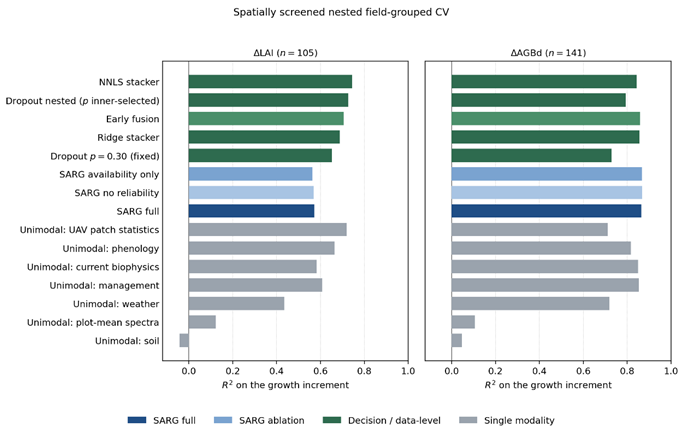
Increment-forecaston the spatially screened sample (v20260920_spatial_verified), matching Table methods.CNN and federated models were not re-fit after screening and are not shown. Bars are nested field-grouped point estimates, not field-bootstrap intervals.
Robustness to Missing Modalities
Table missing withholds one expert at inference, still using the same ExtraTrees experts from v20260920_spatial_verified. Phenology-expert withdrawal does not remove observed Zadoks from gate context (Table withdrawal); it is not complete phenology-sensor loss. The reliability claim is again full gate versus availability-only gating (availability plus agronomic context), not versus a stacker. The nonnegative stacker zeros the dropped coefficient and keeps the intercept (no L1 renormalisation). The masked ridge zeros and L1-renormalises. Dropout is chosen in by inner GroupKFold on the training clients of each outer fold; every fold picked .
On fully observed LAI, NNLS () and nested dropout () beat SARG (). Withholding the phenology expert does not move NNLS (those weights are ) while SARG rises to . Withholding UAV, nested dropout and SARG are similar ( vs ); NNLS collapses to .
On AGBd, availability-only gating is numerically ahead of the full gate when every sensor is present ( vs ; field Wilcoxon ; pooled RMSE , cluster-bootstrap CI to ). Withholding the current biophysics expert, SARG has the lowest pooled point-estimate RMSE () against availability-only (; RMSE , CI to ), nested dropout (), masked ridge () and NNLS (). No field-level Wilcoxon comparison versus availability-only was significant at the unadjusted level (Table avail). Phenology-expert withdrawal leaves the two gates numerically close ( vs , ). Management-expert withdrawal favours availability-only numerically ( vs , ). The gate does reroute when an expert is withheld. The LAI bootstrap-versus-Wilcoxon split is the same as in Section res methods. Versus nested dropout under phenology-expert withdrawal the comparison favours dropout ( vs SARG , unadjusted). Masked-ridge weather-expert withdrawal remains unstable () because weather coefficients are signed; NNLS assigns weather weight , so that withdrawal is a no-op.
Absolute RMSE when one expert is withheld at inference. Phenology-expert withdrawal does not remove observed Zadoks from gate context. Same experts for every column. NNLS masking: zero dropped weights, keep intercept, no renormalisation. Nested dropout:selected inside training folds. Best RMSE in each row in bold. Run v20260920_spatial_verified.
| Withheld expert | SARG | Avail. only | Ridge mask | NNLS mask | Drop. nested |
| LAI | |||||
| None | 1.069 | 1.080 | 0.913 | 0.827 | 0.856 |
| UAV | 1.178 | 1.216 | 1.399 | 1.726 | 1.183 |
| Biophysics expert | 1.072 | 1.081 | 0.972 | 1.033 | 0.941 |
| Phenology expert | 1.430 | 1.429 | 0.923 | 0.827 | 0.897 |
| Weather | 1.063 | 1.077 | 1.054 | 0.827 | 0.820 |
| Soil | 1.070 | 1.079 | 0.930 | 0.854 | 0.827 |
| Spectra | 1.064 | 1.074 | 0.906 | 0.844 | 0.855 |
| Management | 0.961 | 0.974 | 0.948 | 0.827 | 0.876 |
| AGBd () | |||||
| None | 102.4 | 101.1 | 105.2 | 109.9 | 126.0 |
| UAV | 109.8 | 113.3 | 147.5 | 162.6 | 128.6 |
| Biophysics expert | 107.0 | 112.0 | 149.5 | 224.9 | 128.8 |
| Phenology expert | 205.8 | 207.2 | 212.3 | 163.4 | 130.1 |
| Weather | 101.4 | 100.4 | 317.9 | 109.9 | 121.1 |
| Soil | 102.7 | 101.6 | 107.9 | 113.6 | 114.1 |
| Spectra | 104.0 | 101.1 | 113.6 | 109.8 | 112.5 |
| Management | 141.0 | 130.4 | 122.2 | 109.9 | 124.5 |
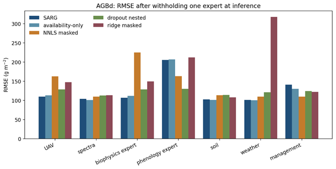
Biomass increment RMSE after withholding one expert at inference. Phenology-expert withdrawal leaves observed Zadoks in the gate context. Comparators are availability-only gating (availability plus agronomic context), masked ridge, nonnegative stacker and nested dropout ridge.
Full reliability gate versus availability-only gating (availability plus agronomic context) on the spatially screened sample. Two summaries are reported and need not agree. PooledRMSE is RMSESARG − RMSEavail on the concatenated out-of-fold rows, using unrounded RMSEs. Theinterval is a field-cluster bootstrap of that same pooled difference (2000 resamples of the twelve season–unit clients). Wilcoxonis an unadjusted signed-rank test of the twelve field-level RMSE differences. A negative pooledRMSE favours SARG. No field-level Wilcoxon comparison was significant at the unadjustedlevel. These tests are exploratory. Small pooled LAI improvements appeared in exploratory bootstrap analyses, but field-level Wilcoxon tests did not establish improvement across fields. Nonsignificance is not evidence of equivalence.
| Target | Condition | SARG | Avail. only | Wilcoxon | Pooled RMSE (CI) |
| AGBd | Fully observed | 102.44 | 101.14 | 0.23 | (, ) |
| Biophysics expert withheld | 107.01 | 111.99 | 0.42 | (, ) | |
| Phenology expert withheld | 205.79 | 207.20 | 0.97 | (, ) | |
| Management withheld | 140.98 | 130.39 | 0.20 | (, ) | |
| LAI | Fully observed | 1.0694 | 1.0798 | 0.47 | (, ) |
| Biophysics expert withheld | 1.0725 | 1.0813 | 0.34 | (, ) | |
| Phenology expert withheld | 1.4302 | 1.4293 | 0.97 | (, ) | |
| Management withheld | 0.9613 | 0.9740 | 0.34 | (, ) |
Walk-Forward Evaluation
Walk-forward split.
Issue time for campaign is the last obs_date among ESUs visited at , so the campaign is issued as one batch. LAI is measured in situ on the observation date (Dimitrov et al. 2026, 2025). Dry above-ground biomass is an oven-dried laboratory mass; TS2AgroBg does not record processing completion dates, so the protocol treats the next-campaign obs_date as the label-availability date. That equation is exact for LAI and optimistic for AGBd if drying lags the field visit. Complete input campaigns stay together: every ESU visited at is training or test, never split by row. At each issue time the training set is every increment row, on any participating client, whose label date is that batch issue date. Imputers, scalers, ExtraTrees experts, stacker coefficients, dropout (inner GroupKFold on those training clients) and the SARG gate are fit on that training set only. No future labels, future covariates or issue-time test rows enter preprocessing or tuning. Using AprilMay labels to train a MayJune forecast is permitted because those May measurements are already in hand under the observation-date convention; mixing AprilMay and MayJune rows of the same campaign in one split is not. After spatial screening, 2016/17 yields two LAI tests (MarchApril, ; AprilMay, ) and three biomass tests (those plus MayJune, ). NovemberMarch ( LAI, biomass kept) has no prior increment labels anywhere and is excluded from within-client temporal evaluation; those labels become training at the March issue. 2017/18 clients have only NovemberApril ( LAI, biomass) and are cold-start tests at the November 2017 issue, trained on all 2016/17 labels (available by June 2017 under the same convention). Table transitions lists the screened counts; row-level assignments and predictions are in the Zenodo reproducibility deposit (Bakır and Salman 2026).
Concatenated walk-forward scores on the screened sample are target-specific (Table wf simple). Pooled RMSE is computed on the concatenated test predictions, not by averaging per-issue . On LAI () the ridge stacker () is numerically ahead of the mean-increment baseline () and of SARG (). On AGBd () the mean increment () beats SARG (), NNLS (), ridge () and persistence (). Every concatenated is negative. Negative means worse than predicting the test-set mean increment; it does not mean that every deployable baseline is better. Ridge therefore records a small numerical LAI RMSE improvement over the mean-increment baseline, while practical or statistically supported temporal forecasting skill remains unestablished on this sample.
A neural federated walk-forward run on the unfiltered sample is in fed; we did not re-fit it after screening.
Walk-forward transition counts on the spatially screened sample. Issue date is the last obs_date of the input campaign. NovemberMarch is training at the March issue, not a test fold.
| Input target | Issue (batch) | LAI | AGBd | 2016/17 role | 2017/18 role |
| NovMar | Nov 2016 | 17 | 21 | excluded (no prior labels) | — |
| MarApr | Mar 2017 | 30 | 30 | test; train on NovMar | — |
| AprMay | Apr 2017 | 30 | 30 | test; train on prior two | — |
| MayJun | May 2017 | 0 | 30 | test (biomass only) | — |
| NovApr | Nov 2017 | 28 | 30 | — | cold-start test |
Concatenated walk-forward RMSE andon the spatially screened sample (v20260920_spatial_verified). Metrics are computed once on all test predictions, not averaged across issue dates. Best RMSE in each column in bold.
| LAI () | AGBd () | |||
| 2-3(lr)4-5 Method | RMSE | RMSE | ||
| Persistence | 2.381 | 452 | ||
| Mean increment | 2.234 | 368 | ||
| Ridge stacker | 2.190 | 428 | ||
| NNLS stacker | 2.284 | 423 | ||
| SARG | 2.365 | 427 | ||
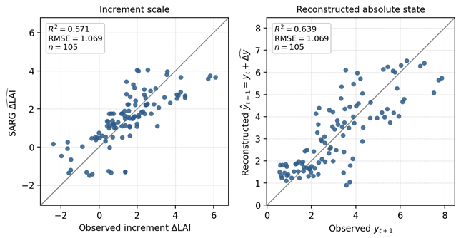
Leaf-area increment forecasts of the full gate under field-out cross-validation on the spatially screened sample (v20260920_spatial_verified;), regenerated from the same out-of-fold predictions as Table param. Left: increment scale (). Right: reconstruction to the absolute next campaign state by Equation reconstruct ().
Discussion
Why the target definition is a methodological choice
The decision that matters most here is the target, not the gate. An of about on next-campaign biomass and for a mean-increment baseline that adds the measured describe residuals of very different variances. They are not a split of skill into seasonal progression. When is observed and clipping is off, : the errors are the same, and only versus changes . The mean-increment baseline still uses the crop. Persistence and a mean growth-rate baseline are in Table param. We did not train a calendar-only, stage-only or horizon-only predictor of , so we have not measured seasonal predictability beyond those controls. Anyone pooling campaigns should report both scales and those baselines. On this dataset the increment also improved absolute-scale LAI, so the more honest parameterisation was not the more pessimistic one.
What the gate contributes, and what it does not
The gate did not win fully observed accuracy. On screened LAI the nonnegative stacker (RMSE ) and nested dropout () beat SARG (). On screened AGBd, no statistically significant difference was detected between SARG and the ridge stacker (RMSE vs ; cluster-bootstrap RMSE CI to ). The median per-field is , about the field-to-field spread—again, not a general claim that is noise.
The reliability claim is tested by the full gate versus availability-only gating (availability plus agronomic context) (Table avail). On fully observed biomass the pooled RMSE is in favour of availability-only (cluster-bootstrap CI to ; field Wilcoxon ). Under withheld biophysics SARG is numerically ahead (pooled RMSE , CI to ; ). Phenology-expert withdrawal is numerically close, with no statistically significant difference detected (); observed Zadoks remains in the gate context, so this is not complete phenology-sensor loss. Management-expert withdrawal leans toward availability-only (). Those summaries need not agree, and the LAI rows of Table avail show they do not: the bootstrap sees a small pooled difference, the field Wilcoxon does not. Expert-withdrawal tests show that the gate reroutes; they do not establish a consistent benefit of typicality and uncertainty.
Comparisons with fixed stackers remain relevant as a second check, not as a substitute. Withholding the current-biophysics expert from biomass, SARG has the lowest pooled RMSE ( vs nested dropout , masked ridge , NNLS ). The paired field test versus nested dropout is not statistically established (). Versus NNLS the comparison is exploratory evidence favouring SARG ( unadjusted), subject to multiplicity. Versus the masked ridge, unadjusted and does not clear . Phenology-expert withdrawal is the reverse: nested dropout vs SARG ( unadjusted). On LAI, withholding the biophysics expert does not favour SARG ( vs nested dropout and masked ridge ). is input typicality: row-wise Spearman tests ignore within-field dependence; soil and weather on biomass have row but field-level Wilcoxon and . UAV typicality does not track error. is a gate input, not an independently validated error predictor on this dataset.
The context ablation, gate-weight tables and end-to-end CNN were not re-fit after screening (hist). Even on the unfiltered sample we did not see a stage-specific robustness, transfer or per-stage accuracy gain. The architecture can depend on ; that is not a finding that stage inputs improve point forecasts here, and the title does not say they do.
The evaluation choice is clearer than the accuracy ranking. The gate has to train on out-of-fold expert predictions, and those predictions have to come from grouped inner folds (Figure inner cv; (Cawley and Talbot 2010; Roberts et al. 2017)). Random inner folds made an earlier SARG look strongest on LAI; grouped folds reverse that ranking. Warm-starting from the L1-normalised intercept-free NNLS of the out-of-fold experts, and leaving and out of weight decay, still helps: otherwise the softmax collapses toward uniform weights. That mapping is not the unconstrained-sum NNLS comparator.
Imagery at campaign scale
On the screened sample, UAV patch statistics are still the best single LAI modality (). A convolutional encoder trained end to end on the older unfiltered sample did not beat those statistics (hist). That is a statement about this campaign size, not about deep image fusion in general, which works at larger scale (Maimaitijiang et al. 2020; Nevavuori, Narra, and Lipping 2019).
Limitations
We have two seasons, six agricultural-unit labels and twelve distinct season–unit clients (206 ESU visits). Grouped folds cannot separate variety from soil from management. Wilcoxon tests on twelve pairs are under-powered and unadjusted; we never named a primary hypothesis. Any-overlap of windows removes large jumps; it does not prove the same sampling area (Table spatial). Majority overlap () repeats the fully observed and missing-modality tables, not walk-forward (Table majority). Under biomass biophysics withdrawal SARG has the lowest pooled RMSE, but the field tests versus availability-only () and nested dropout () are not significant at unadjusted ; versus masked ridge , versus NNLS unadjusted. Most LAI increments sit in early stages. The UAV patches are single-date windows. We did not model harvest yield. Uncertainty enters the gate but is not checked against expert error. The historical typicality diagnostic (hist) is for only, and the field-level correlations mostly do not reject zero. The forecasts are not distribution-calibrated; conformal intervals on the increment are the obvious next step. The older within-field row split is not a prospective test. Neighbouring units are – apart, so field-out CV still leaves spatial dependence. Continuity screening is in Section unification: LAI and biomass transitions were identifier jumps. The federated run in fed standardises concatenated training-client rows and was not re-fit after screening.
Table conclusions collects the headline claims on the spatially screened run, including those that go against the full gate.
Headline findings on the spatially screened run v20260920_spatial_verified. Historical unfiltered analyses are in hist / fed. Paired -values are unadjusted.
| Claim | What it means | Evidence | Take-home |
| Increments are spatially screened | Any-overlap of windows is not identical sampling area. | Displacement : / (LAI), / (biomass). Overlap /; for / retained pairs. Majority repeats fully observed and missing-modality comparisons only (/): nested dropout overtakes NNLS on LAI; availability-only remains ahead of the full gate; biomass biophysics SARG vs avail. , dropout , ridge , NNLS . | Headline tables use any-overlap /. Walk-forward was not repeated under majority overlap. |
| Increment and absolute use different denominators | Reconstruct with measured . | Same residuals; different vs . Mean increment: absolute biomass , AGBd . | Persistence and mean-rate baselines are in Table param. |
| Typicality and uncertainty are unproven | The test of reliability conditioning is full SARG versus availability-only (Table avail). Pooled RMSE and field Wilcoxon are different estimands. | Fully observed biomass pooled RMSE (CI to ), . LAI fully observed (CI to ), . No field Wilcoxon . | Small pooled LAI improvements appeared in exploratory bootstrap analyses, but field-level Wilcoxon tests did not establish improvement across fields. |
| The full gate is not the best fully observed model | NNLS and nested dropout beat SARG on LAI; on biomass, SARG and the ridge stacker are numerically close, with no statistically significant difference detected. | LAI: NNLS / ; nested dropout ; SARG / . AGBd: no-reliability ; availability-only ; SARG ; ridge . | Fully observed accuracy does not justify the full reliability gate. |
| Biophysics withdrawal is exploratory | Compare SARG with availability-only, NNLS and nested dropout under every withheld modality. | Biomass biophysics expert: SARG (lowest point estimate), avail. (), dropout (), masked ridge (), NNLS (). Phenology expert: dropout vs SARG (). | Lowest pooled RMSE under biomass biophysics withdrawal is not a paired win versus availability-only. |
| Walk-forward skill is not established | Concatenate test predictions; include persistence and mean increment. | Screened sample: LAI , ridge vs mean increment vs SARG ; biomass , mean increment vs SARG . All concatenated . | Ridge has a small numerical LAI RMSE gain; temporal skill is not established. Negative is relative to the test-set mean, not to every baseline. Counts: Table transitions / Table wf simple. |
Conclusions
This study asked a bounded question on TS2AgroBg: under what conditions, if any, do typicality and uncertainty improve winter-wheat increment fusion beyond availability-only gating (availability plus agronomic context)? Consecutive visits were kept only when their windows overlap ( LAI, biomass). The full gate was compared with availability-only and no-reliability gates, nonnegative and ridge stackers, and nested expert-dropout, under nested field-grouped cross-fitting, expert withdrawal and concatenated walk-forward. Phenology-aware fusion and increment targets already exist (Liu et al. 2026; Huang et al. 2026; Wang et al. 2026; Senti et al. 2026); the test here is the extra reliability signals and the protocol. Paired tests are exploratory and unadjusted. The evidence is summarised in Table conclusions.
The first two rows of that table are protocol, not ranking. Any-overlap of windows is not a verified plot: median displacements are (LAI) and (biomass), yet LAI and biomass pairs share less than half the window (). Majority overlap () was a sensitivity on /, not the headline sample, and walk-forward was not repeated under that rule. Increment and reconstructed-absolute must be reported together, because they normalise the same residuals by different variances and reconstruction adds the measured . A mean-increment baseline already reaches absolute biomass while remaining near zero on AGBd (); that is a change of denominator, not a split of skill into seasonal progression. Those rows also fix how the later ranking should be read: headline RMSE uses any-overlap /, and a high reconstructed is not evidence that the increment itself was forecast well.
Typicality and uncertainty did not earn a consistent role. On fully observed biomass, availability-only gating had a slightly lower observed RMSE ( versus ), with no statistically significant field-level difference (). Small pooled LAI differences in exploratory bootstraps were not corroborated by field Wilcoxon tests. No field-level comparison of the full gate versus availability-only reached unadjusted under the withdrawal conditions we report. Expert-withdrawal tests show that the gate can reroute; they do not show that the extra reliability signals help.
Fully observed accuracy likewise does not justify the full reliability architecture. A nonnegative stacker is more accurate on LAI (RMSE versus ). On AGBd, SARG and the ridge stacker are numerically close, with no statistically significant difference detected. Among the evaluated gate variants, availability-only gating therefore remains a simpler alternative. It is not identified as best under every withdrawal: withholding the current-biophysics expert leaves SARG with the lowest pooled biomass RMSE ( versus availability-only , ), while phenology-expert withdrawal favours nested dropout over SARG. Phenology-expert withdrawal is not complete loss of phenological information, because observed Zadoks remains in the gate context.
Concatenated walk-forward, the last row of Table conclusions, does not establish usable next-campaign skill on this sample ( LAI, biomass). Ridge records a small numerical LAI RMSE gain over the mean-increment baseline ( versus ); the mean increment is ahead on AGBd ( versus SARG ); every concatenated is negative relative to the test-set mean, which does not imply that every deployable baseline is better.
The contribution is therefore comparative and methodological rather than a claim of operational advancement: spatially screened increments, an honest nested protocol, and a direct test of reliability conditioning against availability-only gating. What would change the answer is a reliability score that tracks expert error at field level; conformal intervals on the increment; more dates and plots before a learned image encoder; a remotely sensed if an absolute-state pipeline is required; and public soil and weather layers in place of campaign pits and station files.
Historical unfiltered analyses
Gate-weight tables, typicality–error scatter, the reduced-input ladder and the end-to-end CNN comparison use the older unfiltered sample. We did not re-fit them after spatial screening, and they are not part of the main results; the tables and figures are in the Zenodo deposit named in the Data Availability statement (Bakır and Salman 2026).
On that unfiltered sample the biomass gate still favoured phenology (–) with management at –. November 2017 shifted mass from phenology to management on biomass and from UAV to management on LAI. The use_context=False ablation did not reduce pooled skill (LAI ; biomass ). Each reduced-input rung retrains SARG; reconstruction Equation reconstruct still uses measured . The same 161 patches produced the best single LAI-increment modality as 31 statistics and did not improve as a CNN trained on roughly 90 examples (). That CNN is the neural alternative labelled in Figure architecture, not the ExtraTrees protocol of the main tables.
Historical Federated Optimisation Simulation
A neural federated walk-forward and personalisation run on the unfiltered historical sample is in the same Zenodo deposit (Bakır and Salman 2026). We did not re-fit it after screening. Preprocessing still needs every training-client row in one place: medians, feature scales and image normalisation are fitted on the concatenated training-client table (PersonalizedFederatedFusion.fit calls _Preprocessor.fit on that table). Local updates are then averaged with FedAvg (McMahan et al. 2017), optionally leaving the gate local. That is federated optimisation with centralised preprocessing, not a field-local training pipeline. Walk-forward neural federation did not produce a usable increment (2016/17 -weighted RMSE – on LAI; – on AGBd). The 2017/18 cold-start biomass case (FedAvg RMSE , ) remains worse than predicting the test-set mean.
References
- Abouaomar, Anas; El Hanjri, Mohammed; Kobbane, Abdellatif; Laouiti, Anis; Nafil, Khalid. Hierarchical Federated Learning for Crop Yield Prediction in Smart Agricultural Production Systems. International Conference on Wireless Networks and Mobile Communications (WINCOM), 2025. [Google Scholar] [CrossRef]
- Bakır, Murat Gökşin; Salman, Yücel Batu. Reliability-Gated Multimodal Fusion. Zenodo (dataset), version 1, CC BY 4.0; 2026. [Google Scholar] [CrossRef]
- Baltrušaitis, Tadas; Ahuja, Chaitanya; Morency, Louis-Philippe. Multimodal Machine Learning: A Survey and Taxonomy. IEEE Trans. Pattern Anal. Mach. Intell. 2019, 41(2), 423–43. [Google Scholar] [CrossRef] [PubMed]
- Castanedo, Federico. A Review of Data Fusion Techniques. Sci. World J. 2013, 2013, 704504. [Google Scholar] [CrossRef] [PubMed]
- Cawley, Gavin C.; Talbot, Nicola L. C. On over-Fitting in Model Selection and Subsequent Selection Bias in Performance Evaluation. J. Mach. Learn. Res. 2010, 11, 2079–2107. [Google Scholar]
- Chen, Tianqi; Guestrin, Carlos. XGBoost: A Scalable Tree Boosting System. 22nd ACM SIGKDD International Conference on Knowledge Discovery and Data Mining, 2016; pp. 785–94. [Google Scholar] [CrossRef]
- Dimitrov, Petar; Kamenova, Ilina; Roumenina, Eugenia; Filchev, Lachezar; Ilieva, Iliana; Jelev, Georgi; Gikov, Alexander; et al. Estimation of Biophysical and Biochemical Variables of Winter Wheat Through Sentinel-2 Vegetation Indices. Bulg. J. Agric. Sci. 2019, 25(5), 819–32. Available online: https://www.agrojournal.org/25/05-01.pdf.
- Dimitrov, Petar; Roumenina, Eugenia; Jelev, Georgi; Filchev, Lachezar; Gikov, Alexander; Kamenova, Ilina; Ilieva, Iliana; et al. In-Situ and UAV Dataset with Crop and Soil Parameters Obtained from Winter Wheat Fields. Zenodo (dataset) CC BY 4.0. 2025, version 1.0.0. [Google Scholar] [CrossRef]
- ———, et al. In Situ Crop and Soil Data and UAV Imagery from Winter Wheat Fields in a Bulgarian Site. Data 2026, 11(2), 35. [Google Scholar] [CrossRef]
- Durrant, Aiden; Markovic, Milan; Matthews, David; May, David; Enright, Jessica; Leontidis, Georgios. The Role of Cross-Silo Federated Learning in Facilitating Data Sharing in the Agri-Food Sector. Comput. Electron. Agric. 2022, 193, 106648. [Google Scholar] [CrossRef]
- Field, Christopher A.; Welsh, Alan H. Bootstrapping Clustered Data. J. R. Stat. Soc. Ser. B 2007, 69(3), 369–90. [Google Scholar] [CrossRef]
- Geurts, Pierre; Ernst, Damien; Wehenkel, Louis. Extremely Randomized Trees. Mach. Learn. 2006, 63(1), 3–42. [Google Scholar] [CrossRef]
- Hall, David L.; Llinas, James. An Introduction to Multisensor Data Fusion. Proc. IEEE 1997, 85(1), 6–23. [Google Scholar] [CrossRef]
- Han, Zongbo; Zhang, Changqing; Fu, Huazhu; Zhou, Joey Tianyi. Trusted Multi-View Classification. International Conference on Learning Representations (ICLR), 2021; Available online: https://openreview.net/forum?id=DNz4sY0Uf45.
- Huang, Zijing; Lee, Won Suk; Ampatzidis, Yiannis; Agehara, Shinsuke; Peres, Natalia A. PheMuT: A Phenology-Informed, Multi-Modal Time-Series Model for Strawberry Yield Forecasting. Comput. Electron. Agric. 2026, 244, 111526. [Google Scholar] [CrossRef]
- IUSS Working Group WRB. World Reference Base for Soil Resources 2014: International Soil Classification System for Naming Soils and Creating Legends for Soil Maps. Update 2015. In World Soil Resources Reports 106; Food: Rome; Agriculture Organization of the United Nations, 2015; Available online: https://openknowledge.fao.org/handle/20.500.14283/i3794en.
- Jacobs, Robert A.; Jordan, Michael I.; Nowlan, Steven J.; Hinton, Geoffrey E. Adaptive Mixtures of Local Experts. Neural Comput. 1991, 3(1), 79–87. [Google Scholar] [CrossRef] [PubMed]
- Kendall, Alex; Gal, Yarin. What Uncertainties Do We Need in Bayesian Deep Learning for Computer Vision? Adv. Neural Inf. Process. Syst. (NeurIPS) 2017, 5574–84. [Google Scholar]
- Khaleghi, Bahador; Khamis, Alaa; Karray, Fakhreddine O.; Razavi, Saiedeh N. Multisensor Data Fusion: A Review of the State-of-the-Art. Inf. Fusion 2013, 14(1), 28–44. [Google Scholar] [CrossRef]
- van Klompenburg, Thomas; Kassahun, Ayalew; Catal, Cagatay. Crop Yield Prediction Using Machine Learning: A Systematic Literature Review. Comput. Electron. Agric. 2020, 177, 105709. [Google Scholar] [CrossRef]
- Liu, Qingkai; Jing, Haitao; Wen, Xueying; Wu, Xuan; Yan, Long; Yang, Qing; Jia, Siyu; Guo, Siyu; Fan, Fan; Jin, Xiuliang. Soybean Phenological Stage Identification Based on Multimodal Data and a Dynamic Gating Fusion Model. Smart Agric. Technol. 2026, 13, 101827. [Google Scholar] [CrossRef]
- Loshchilov, Ilya; Hutter, Frank. Decoupled Weight Decay Regularization. International Conference on Learning Representations (ICLR), 2019; Available online: https://openreview.net/forum?id=Bkg6RiCqY7.
- Ma, Mengmeng; Ren, Jian; Zhao, Long; Tulyakov, Sergey; Wu, Cathy; Peng, Xi. SMIL: Multimodal Learning with Severely Missing Modality. AAAI Conf. Artif. Intell. 2021, 35, 2302–10. [Google Scholar] [CrossRef]
- Maimaitijiang, Maitiniyazi; Sagan, Vasit; Sidike, Paheding; Hartling, Sean; Esposito, Flavio; Fritschi, Felix B. Soybean Yield Prediction from UAV Using Multimodal Data Fusion and Deep Learning. Remote Sens. Environ. 2020, 237, 111599. [Google Scholar] [CrossRef]
- McMahan, H. Brendan; Moore, Eider; Ramage, Daniel; Hampson, Seth; Agüera y Arcas, Blaise. Communication-Efficient Learning of Deep Networks from Decentralized Data. 20th International Conference on Artificial Intelligence and Statistics Proceedings of Machine Learning Research 2017, 54, 1273–82. Available online: https://proceedings.mlr.press/v54/mcmahan17a.html.
- Mukherjee, Anwesha; Buyya, Rajkumar. Federated Learning Architectures: A Performance Evaluation with Crop Yield Prediction Application. Softw. Pract. Exp. 2025, 55(7), 1165–84. [Google Scholar] [CrossRef]
- Nevavuori, Petteri; Narra, Nathaniel; Lipping, Tarmo. Crop Yield Prediction with Deep Convolutional Neural Networks. Comput. Electron. Agric. 2019, 163, 104859. [Google Scholar] [CrossRef]
- Roberts, David R.; Bahn, Volker; Ciuti, Simone; Boyce, Mark S.; Elith, Jane; Guillera-Arroita, Gurutzeta; Hauenstein, Severin; et al. Cross-Validation Strategies for Data with Temporal, Spatial, Hierarchical, or Phylogenetic Structure. Ecography 2017, 40(8), 913–29. [Google Scholar] [CrossRef]
- Roumenina, Eugenia; Jelev, Georgi; Dimitrov, Petar; Filchev, Lachezar; Kamenova, Ilina; Gikov, Alexander; Banov, Martin; Krasteva, Veneta; Kercheva, Milena; Kolchakov, Viktor. Qualitative Evaluation and Within-Field Mapping of Winter Wheat Crop Condition Using Multispectral Remote Sensing Data. Bulg. J. Agric. Sci. 2020, 26(6), 1129–42. Available online: https://www.agrojournal.org/26/06-05.pdf.
- Senti, Dominik; Turkoglu, Mehmet Ozgur; Volpi, Michele; Aasen, Helge. Learning to Forecast Crop Growth from Earth Observation Data. arXiv 2026, arXiv:2608.14281. [Google Scholar]
- Shazeer, Noam; Mirhoseini, Azalia; Maziarz, Krzysztof; Davis, Andy; Le, Quoc; Hinton, Geoffrey; Dean, Jeff. Outrageously Large Neural Networks: The Sparsely-Gated Mixture-of-Experts Layer. International Conference on Learning Representations (ICLR), 2017; Available online: https://openreview.net/forum?id=B1ckMDqlg.
- Verrelst, Jochem; Camps-Valls, Gustau; Muñoz-Marí, Jordi; Rivera, Juan Pablo; Veroustraete, Frank; Clevers, Jan G. P. W.; Moreno, José. Optical Remote Sensing and the Retrieval of Terrestrial Vegetation Bio-Geophysical Properties – a Review. ISPRS J. Photogramm. Remote Sens. 2015, 108, 273–90. [Google Scholar] [CrossRef]
- Wang, Baoju; Zhu, Junke; Sun, Shuai; Zhang, Lechun; Yan, Yu; Wang, Huizheng; Yang, Weiguang; Lan, Yubin. Multimodal Remote Sensing Combination for Maize LAI Estimation: Stacking Model Development and Phenology-Specific Feature Sensitivity Analysis. Artif. Intell. Agric. 2026, 16(2), 873–88. [Google Scholar] [CrossRef]
- Weiss, Marie; Baret, Frédéric; Smith, G. J.; Jonckheere, Inge; Coppin, Pol. Review of Methods for in Situ Leaf Area Index (LAI) Determination: Part II. Estimation of LAI, Errors and Sampling. Agric. For. Meteorol. 2004, 121(1–2), 37–53. [Google Scholar] [CrossRef]
- Wolpert, David H. Stacked Generalization. Neural Netw. 1992, 5(2), 241–59. [Google Scholar] [CrossRef]
- Xue, Zihui; Marculescu, Radu. Dynamic Multimodal Fusion. IEEE/CVF Conference on Computer Vision and Pattern Recognition Workshops (CVPRW), 2023; pp. 2575–84. [Google Scholar] [CrossRef]
- Yang, Qiang; Liu, Yang; Chen, Tianjian; Tong, Yongxin. Federated Machine Learning: Concept and Applications. ACM Trans. Intell. Syst. Technol. 2019, 10((2): 12), 1–19. [Google Scholar] [CrossRef]
- Zadoks, J. C.; Chang, T. T.; Konzak, C. F. A Decimal Code for the Growth Stages of Cereals. Weed Res. 1974, 14(6), 415–21. [Google Scholar] [CrossRef]
- Zhou, X.; Zheng, H. B.; Xu, X. Q.; He, J. Y.; Ge, X. K.; Yao, X.; Cheng, T.; Zhu, Y.; Cao, W. X.; Tian, Y. C. Predicting Grain Yield in Rice Using Multi-Temporal Vegetation Indices from UAV-Based Multispectral and Digital Imagery. ISPRS J. Photogramm. Remote Sens. 2017, 130, 246–55. [Google Scholar] [CrossRef]
Disclaimer/Publisher’s Note: The statements, opinions and data contained in all publications are solely those of the individual author(s) and contributor(s) and not of MDPI and/or the editor(s). MDPI and/or the editor(s) disclaim responsibility for any injury to people or property resulting from any ideas, methods, instructions or products referred to in the content. |
© 2026 by the authors. Licensee MDPI, Basel, Switzerland. This article is an open access article distributed under the terms and conditions of the Creative Commons Attribution (CC BY) license (http://creativecommons.org/licenses/by/4.0/).
Copyright: This open access article is published under a Creative Commons CC BY 4.0 license, which permit the free download, distribution, and reuse, provided that the author and preprint are cited in any reuse.