

Submitted:
12 October 2026
Posted:
13 October 2026
You are already at the latest version
Abstract
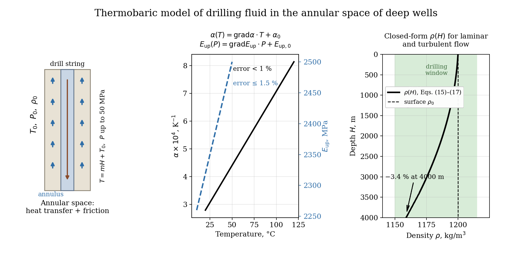
Accurate prediction of drilling-fluid density and hydraulic parameters under downhole conditions is essential for the safe drilling of deep and high-pressure/high-temperature (HP/HT) wells, in which the window between pore and fracture pressures is often narrow. This study develops a thermobaric model of drilling fluid in the annular space, where heat exchange and hydraulic resistance are most intense. The total differential of fluid volume with respect to temperature and pressure was combined with laboratory data for wellbore water obtained on a rig simulating downhole conditions. Correlation analysis showed that, at pressures above 10 MPa, the thermal expansion coefficient is a linear function of temperature over the range 0–100 °C (error < 1%). At the same time, the isothermal bulk modulus is a linear function of pressure at temperatures of 5 °C and above within the in-vestigated range of 0.5–8 MPa (error ≤ 1.5%) and is extrapolated to downhole pressures. Integration of the resulting differential equation yielded closed-form equations for fluid density versus depth for laminar and turbulent flow. Combined with drilling-window constraints, they form systems for selecting fluid properties and circulation velocity that prevent lost circulation, influx and pipe sticking. The model is a lightweight phys-ics-based tool for hydraulic design and real-time monitoring.
Keywords:
drilling fluid
; thermobaric model
; annular space
; HP/HT wells
; density
; thermal expansion coefficient
; isothermal compressibility
; equivalent circulating density
; drilling window
1. Introduction
Deep and ultra-deep drilling, as well as the development of high-temperature and high-pressure fields, are key directions in the oil and gas industry. The efficiency and safety of drilling critically depend on the properties of the drilling fluid – a multifunctional dispersed system that performs a number of vital tasks: cuttings transport, maintaining hydrostatic pressure in the well, cooling the bit, and stabilizing the borehole wall [1,2,3,4].
During circulation, the drilling fluid is subjected to extreme thermobaric loads [4,5,6,7]. With increasing depth, temperature and pressure rise significantly, inevitably leading to changes in its physicochemical and structural-mechanical properties [8,9,10,11,12]. An increase in temperature can initiate thermal decomposition of components, coagulation, polymer degradation and, consequently, a sharp decrease in viscosity and rheological stability. At the same time, an increase in pressure usually causes compression of the dispersed phase and a reduction in interparticle distance, which, conversely, can lead to an increase in viscosity. These oppositely directed effects of and interact in a complex nonlinear manner. Accurate prediction of rheological parameters under HP/HT (high-pressure/high-temperature) conditions is a critical task for drilling control [12,13,14,15,16].
Field and laboratory evidence consistently shows that these effects cannot be neglected. Downhole pressure and temperature measurements in an offshore well drilled with a synthetic-based fluid demonstrated that the static and circulating density profiles deviate markedly from the surface-measured mud weight, because the fluid is heated and compressed simultaneously along the wellbore [5]. Systematic laboratory studies of base oils, brines and complete drilling fluids at extreme temperatures and pressures confirmed that the density of the liquid phase can change by several percent over the ranges typical of deep wells, with oil-based systems being noticeably more compressible and more thermally expansible than water-based ones [17,18]. Compositional models, in which the density of the whole fluid is assembled from the volumetric behaviour of its liquid components while the solids are treated as practically incompressible, have therefore become a common engineering approach [19]. More recently, automated laboratory set-ups have been developed to measure the pressure and temperature dependence of drilling-fluid density directly [20], and dedicated density–pressure–temperature formulations for the aqueous phase have been proposed for real-time HP/HT applications [21]. The reference equation of state for water [22] provides a rigorous thermodynamic basis for such formulations, but it is too cumbersome to be embedded directly in closed-form hydraulic calculations.
In parallel, a large body of work has addressed the prediction of downhole density with data-driven methods, including support vector machines, radial basis function and feed-forward neural networks, gradient-boosted trees and hybrid algorithms optimised by metaheuristics [23,24,25,26,27]. These models reproduce laboratory datasets with high accuracy, but their coefficients have no direct physical meaning, their reliability outside the range of the training data is uncertain, and they do not by themselves ensure consistency between density, pressure and flow regime along the wellbore. A physically transparent model with a small number of measurable parameters therefore remains of practical interest, both as a stand-alone design tool and as a physical constraint for data-driven approaches.
Heat and mass transfer processes, as well as hydraulic losses, are most intense in the annular space – the narrow annular gap between the drill string and the borehole wall (or casing) [28,29,30,31,32]. Here, the greatest increase in fluid temperature occurs, and hydraulic resistance (pressure drop) is formed, which directly affects such parameters as: cuttings removal efficiency, the magnitude of hydrodynamic pressures affecting borehole stability and preventing fluid influx, and circulation energy costs [33,34,35].
Incorrect accounting or inaccurate prediction of rheological and hydraulic parameters in the annulus under HP/HT conditions can lead to: reduced rate of penetration, difficulties in cuttings transport, increased accident rate (sticking, caving, lost circulation), and critical errors in cementing program design.
These consequences are most severe in wells with a narrow drilling window, where the admissible range of the equivalent circulating density (ECD) between the pore (or collapse) pressure gradient and the fracture pressure gradient may amount to only a few tens of kilograms per cubic metre. Under such conditions, an error in the downhole density or in the annular frictional pressure loss of the same order as the thermobaric correction itself can shift the bottomhole pressure outside the safe interval [34,36]. Real-time ECD estimation has therefore attracted considerable attention, ranging from hydraulic models calibrated against distributed downhole pressure data [35] to machine-learning estimators trained on surface drilling parameters [37].
Early works in the field of modelling rheological properties of drilling fluids focused on simple models: Bingham-Plastic and Power-Law. Currently, the generally accepted standard for most modern drilling fluids (especially oil-based ones) is the Herschel-Bulkley model [38]:
Historically, simple rheological models were widely used to describe drilling fluid flow. The Bingham model assumes a shear stress that must be overcome to initiate flow. While the Bingham model describes behaviour at high shear rates well, it is often inadequate at low shear rates. The Power-Law model, on the contrary, describes low shear rates better but does not have an explicit yield stress.
In modern practice, especially when working with polymer-based and oil-based muds, the Herschel–Bulkley (HB) model has become the gold standard, combining the advantages of both [2,38,39,40,41,42,43,44]. Using three parameters, this model provides the best approximation of experimental data over a wide range of shear rates. However, the true complexity lies not in the choice of the model, but in accurate determination how these three key parameters change under the extreme thermobaric conditions of deep wells.
The temperature and pressure dependence of the rheological parameters has been investigated experimentally for water-based, oil-based, formate and geothermal drilling fluids [16,45,46]. As a rule, the yield stress and the consistency index decrease with increasing temperature and increase with pressure, whereas the flow behaviour index changes only moderately; the magnitude of these trends, however, depends strongly on the fluid composition. The measured parameters are also sensitive to the viscometer geometry, and shear-rate corrections are required when Herschel–Bulkley fluids are tested in Couette viscometers [47]. Alternative multi-parameter rheological models, such as the vom Berg and Hahn–Eyring models, have been proposed to describe specific fluid systems more accurately [48,49], and in situ thermal conditions have been shown to affect surge and swab pressures significantly [50].
Several authors have proposed models that include both factors, often using multiplicative corrections. A typical approach consists of separate calculation of temperature and pressure factors [51,52,53,54,55,56]:
where is the thermal factor and is the baric factor.
Most empirical and semi-empirical models that account for the influence of and on rheological parameters are either highly specialised (applicable only to a specific fluid type or range) or use linear or additive dependencies, which do not reflect the complex mechanism of structural changes. Comprehensive mathematical models capable of adequately describing the nonlinear interdependence of rheological parameters on simultaneously acting and are insufficiently developed, especially at high shear rates characteristic of the annulus. Hydraulic calculations in the annulus require integration of the equations of motion in the annular gap, which is complicated by the following factors [57,58,59,60,61]: non-Newtonian flow behaviour (use of the Herschel–Bulkley model), annular eccentricity (non--concentric arrangement of strings), non-isothermal flow (significant temperature gradient along the annulus), and mixed flow regime (transition from laminar to turbulent flow).
Existing hydraulic models often neglect a detailed account of changes in rheological parameters along the annulus due to temperature and pressure effects, which leads to significant errors in pressure loss calculations and, consequently, in the estimation of bottomhole hydrodynamic pressures.
A further motivation for compact thermobaric models comes from the rapid development of automated drilling-fluid monitoring. Inline and skid-based systems that measure density, rheology and other properties at the rig site at intervals of several minutes are now available and have been tested in field conditions [62,63], including HP/HT gas wells drilled with managed pressure drilling (MPD) systems [64,65]. The authors’ previous work has addressed measurement devices, improved viscometric procedures and software–hardware complexes for continuous monitoring of drilling-fluid properties [31,32,66,67,68]. However, all such systems measure the fluid at surface conditions. To use these data for downhole pressure management, the measured values must be converted to the actual temperature and pressure at respective depth, which requires a model that is both physically sound and computationally inexpensive.
The annular space is a critical modelling object. It is the zone, where temperature gradients are most pronounced and where bottomhole pressure has the greatest impact on well stability. The drilling fluid is the most important component of the drilling system, responsible for cuttings transport, borehole wall stabilisation and, most importantly, for bottomhole pressure control. When drilling deep wells or wells with high pressure and high temperature, traditional surface measurements of rheology and density lose their accuracy. The plastic viscosity and density can change significantly under the pressure (compaction) and temperature (thermal expansion). Inaccurate measurement of rheological parameters in the annulus leads to erroneous pressure loss calculations, thereby narrowing the drilling window. Thus, the aim of this work is to develop a mathematical model for accurate prediction of rheological and hydraulic parameters in the annulus as functions of depth .
The novelty of the present study covers the following: (i) the linearity of the thermal expansion coefficient with respect to temperature and of the isothermal bulk modulus with respect to pressure is verified statistically for the range of conditions typical of wells deeper than 1000 m; (ii) on this basis, the differential equation of volume change is integrated in closed form along the annulus, with the local hydraulic resistance included separately for laminar and turbulent flow; and (iii) the resulting density equations are combined with the drilling-window constraints into systems that can be solved directly for the admissible circulation velocity and fluid parameters.
2. Materials and Methods
The coefficient α of thermal expansion (with respect to temperature change), , and the isothermal compressibility coefficient β (with respect to pressure change), , characterize the change in fluid volume. Thus, the change in fluid volume depends on temperature and pressure :
V=V(P,T).
From mathematical analysis, the total differential of the function of two variables describes its change:
Dividing by gives:
Here, is the coefficient of thermal expansion, and is the isothermal compressibility coefficient. Hence, it can be written as follows:
In wells deeper than 1000 m, the temperature exceeds 20 °C and pressure exceeds 10 MPa. Therefore, the functions and must be determined. First, we evaluate these dependencies for linearity. If linear, we derive the explicit relations. We consider at constant and at constant . The results are combined with Eq. (6). The linearity assessment was performed using an experimental rig shown in Figure 1, filled with wellbore water, and the conclusions are considered valid for water-based drilling fluids.
2.1. Experimental Setup and Measurement Procedure
The laboratory rig shown in Figure 1 reproduces the thermobaric conditions of the annular space. The wellbore simulator body (6), closed by the top cover (17), contains a drill-string model (7, 20, 21) suspended on a rod (16) and surrounded by the test fluid (8), so that an annular gap is formed between the string and the simulator wall. The temperature is controlled by the circulating temperature-control liquid (3), which is heated by the electric heater (5) and circulated by the pump (12) driven by the motor (13) through the control valve (14); the thermal insulation pad (2) reduces heat losses to the rig base. The pressure is generated by the hydraulic press (9) connected to the simulator through the high-pressure tube (9a) and the press coupling (15). The tube (11) connecting the tank (4) with the simulator makes it possible to reproduce water influx. Temperature and pressure are measured by the thermometer (19) and the pressure gauge (22); all signals are collected by the microcontroller (25) and transmitted via the communication cable (24) to the process-control computer (10). The rig allows tests at temperatures from 1 to 110 °C and at pressures up to 50 MPa; the thermal expansion series were run at 0.1, 10, 20 and 50 MPa and the compressibility series at 0.5–8 MPa, as indicated in Table 1 and Table 3.
The thermal expansion coefficient was determined at constant pressure by raising the temperature from 0 to 100 °C in steps of 10 °C. The series were repeated at pressures of 0.1, 10, 20 and 50 MPa, and results are collected in Table 1 and discussed in the next section. The isothermal compressibility was determined at constant temperature by raising the pressure in the steps 0.5, 1, 2, 4 and 8 MPa. These series were repeated at temperatures of 0, 5, 10, 15 and 25 °C. After each step, the readings were held for 15 min until the temperature and the pressure had stabilised, and the corresponding change in the fluid volume was recorded. Each series was repeated three times, and the arithmetic mean values were used in the correlation analysis. The temperature was measured with a laboratory thermometer with a scale interval of 1 °C and a maximal error of ±0.5 °C. For the pressure, a gauge of accuracy class 0.6 was used with an upper measuring limit of 60 MPa, i.e. with a limit of error of ±0.36 MPa.
The density of the test fluid at surface conditions, ρ0, was determined with an ABR-1 hydrometer. The permissible additional error of this instrument does not exceed 2 kg/m³ for every 10 °C change of the test-solution temperature from 20±2 °C, and 10 kg/m³ for every 10 °C change caused by climatic environmental factors. The hydrometer was calibrated with distilled water at 20±5 °C, for which the reading must equal 1000 kg/m³. These uncertainties propagate directly into ρ0 and, therefore, into the density profiles calculated with the model.
The linearity analysis was performed with wellbore water. This choice is justified by the fact that, in water-based drilling fluids, the liquid phase determines the volumetric response to temperature and pressure. The solid phase consisting of clay and weighting material is practically incompressible and has a thermal expansion coefficient about an order of magnitude lower than that of water. The same principle underlies compositional density models [17,19].
2.2. Linear Dependence of the Thermal Expansion Coefficient α=α(T) at Constant Phydr for Wellbore Water
Experimental values of the thermal expansion coefficient α× for wellbore water at different temperatures and pressures are given in Table 1. The measured values of Table 1 agree with the reference equation of state for water [22] within about 1% over most of the range investigated. For oil-based and synthetic fluids, whose base liquids are considerably more compressible, the parameters must be determined separately (see Section 4.4).
To evaluate linearity of , the correlation coefficient is calculated as:
The correlation coefficient lies in the range , and its absolute value can be interpreted as follows:
– excellent correlation,
– good correlation,
– satisfactory correlation,
– no linear relationship.
For high accuracy, the least-squares method is recommended only when . Using Table 1 and Eq. (7), the correlation coefficients and linearity assessments are as follows:

Table 2.
Correlation coefficients for .
| Pressure , MPa | rc | Assessment |
|---|---|---|
| 0.1 | 0.9803 | NOT LINEAR |
| 10 | 0.9899 | LINEAR |
| 20 | 0.9906 | LINEAR |
| 50 | 0.994 | LINEAR |
Higher pressure reduces the error of the linear relationship between temperature and thermal expansion coefficient. In wells deeper than 1000 m, pressure exceeds 10 MPa and temperature exceeds 20 °C, so is linear for wellbore water with an error less than 1 %.
For a linear dependence, the derivative is constant. Since the above evaluation shows that is constant for wellbore water in deep wells:
Here (in ) is the gradient of the thermal expansion coefficient of the drilling fluid at a given pressure, determined in the laboratory from:
is constant for a given drilling fluid. Integrating (8) gives:
Equations (8–10) are valid only for temperatures above 20 °C and pressures above 10 MPa, i.e., for well depths greater than 1000 m.
2.3. Linear Dependence of the Isothermal Compressibility Coefficient
Empirical values of the isothermal compressibility coefficient β, , for wellbore water are given in Table 3. These measurements were performed at pressures from 0.5 MPa to 8 MPa and temperatures from 0 °C to 25 °C, whereas the thermal expansion data of Table 1 cover pressures up to 50 MPa and temperatures up to 100 °C. The extrapolation of the resulting linear law to the pressures encountered in deep wells.
Using Eq. (7), the correlation coefficients rc for are calculated and collected in Table 4. However, better linear correlation is found for the isothermal bulk modulus as a function of pressure, as shown in Table 5.
Within the investigated range, a higher temperature reduces the error of the linear relationship between pressure and the isothermal bulk modulus: at temperatures of 5 °C and above, the linearity criterion (7) is satisfied, whereas at 0 °C it is not. Since the temperature of a well deeper than 1000 m exceeds 20 °C, the linear approximation is adopted in the form:
where , MPa. Then:
Integrating:
Hence:
Equations above are valid for temperatures T > 20 °C and pressure , corresponding to wells deeper than 1000 m.
2.4. Pressure Balance During Circulation
The bottomhole pressure during circulation is given by:
where is the hydrostatic pressure (MPa), the frictional pressure loss in the annulus (MPa), and the surface pressure (MPa). Because the fluid moves upward in the annulus, the frictional losses increase the bottomhole pressure, so that the equivalent circulating density always exceeds the static one; this sign convention is used consistently in Equations (23), (29)–(36). The hydrostatic pressure is:
with the drilling fluid density, kg/m³; gravity acceleration, m/s²; and the well depth, m. The frictional loss is described by the Darcy-Weisbach equation:
Here is the friction factor; the mean flow velocity, m/s; and the hydraulic diameter of the annulus, m; with the wellbore diameter and the outer drill pipe diameter, respectively. The Reynolds number in the annulus is:
where is the dynamic viscosity, Pa·s; and is the kinematic viscosity, m²/s.
For laminar flow (), , and Eq. (17) becomes:
For turbulent flow in smooth pipes (), the Blasius approximation gives . Substituting into Eq. (17):
2.5. Temperature and Pressure Profiles
The geothermal gradient is assumed constant:
Thus, the temperature at depth is:
where is the surface temperature, K. From the pressure balance (15)–(17), the pressure at depth can be expressed as:
After differentiating, it becomes as follows:
2.6. Density Model for Circulating Conditions
Substituting (24) into the differential volume change Eq. (6), it appears as follows:
Using the linear relations (10) for α and (13) for Eup , and after algebraic manipulation (see Appendix A), the density at depth is obtained as:
where the constants are defined as:
and is the fluid density at surface conditions ().
2.6.1. Laminar Flow Regime
Insert the laminar expression for ξ derived from (19):
with from the Frenkel-Andrade equation, where A is the pre-exponential factor, Pa·s; E is the activation energy of viscous flow, and k is the Boltzmann constant (or the universal gas constant when E is expressed per mole). Substituting into (26) and raising to the power q yields the algebraic equation:
with
The inequality ensures laminar flow at .
2.6.2. Turbulent Flow Regime
Using the turbulent expression (20) and , the hydraulic resistance term becomes:
Inserting this into (26) and raising to the power q leads to following:
where
The inequality enforces turbulent flow at .
2.7. Drilling Window and Safe Operating Conditions
To avoid formation fracture (lost circulation) or collapse (influx), the bottomhole pressure must satisfy the following:
where , with the abnormality coefficient and water density, while . Combining this with the appropriate flow regime equation gives the final coupled systems.
For laminar flow:
For turbulent flow:
The constants in (29) and (32) are those defined for the respective regimes above. These systems allow one to select the flow velocity and fluid parameters that maintain a safe downhole pressure while keeping the desired flow regime in the annulus.
All models are valid for T > 20 °C and , i.e., for well depths greater than 1000 m, with an overall error not exceeding ±1.5 % when the laboratory data are accurate.
2.8. Determination of Model Parameters
The model contains three groups of input parameters shown in Table 6. Geometric and operational parameters, i.e. the well depth H, the hydraulic diameter dh, the mean annular velocity v and the surface pressure P0, are known from the well design and the drilling programme. The thermal parameter m is the temperature gradient along the annulus, which can be estimated from offset-well data or from downhole temperature measurements [4]. The fluid parameters are determined in the laboratory. The coefficients gradα(T) and α(T0, P0) are obtained by least-squares fitting of the measured α–T data at the pressure of interest, and grad(Eup) and Eup(P0, T0) by fitting of the Eup–P data at the temperature of interest; in both cases, the linear approximation is accepted only if |rc| ≥ 0.985, see Equation (7). The constants A and E of the Frenkel–Andrade equation are found from viscosity measurements at no fewer than three temperatures by linear regression of ln μ against 1/T, whose slope equals E/k and whose intercept equals ln A. Finally, ρ0 is the density measured at surface conditions.
2.9. Numerical Solution Procedure
For a given depth, Equations (29) and (32) are nonlinear algebraic equations with respect to ρ, which do not admit an explicit solution for an arbitrary exponent q. They are solved numerically by the Newton–Raphson method, with the surface density ρ0 used as the initial approximation; because the density changes by only a few percent along the wellbore, convergence to a relative tolerance of 10−6 is usually achieved within a few iterations. The calculation proceeds as follows: (1) the temperature at depth H is calculated from Equation (22) and the viscosity from the Frenkel–Andrade equation; (2) a flow regime is assumed, and the corresponding equation, (29) or (32), is solved for ρ; (3) the Reynolds-number inequality of the selected system is checked, and if it is violated, the calculation is repeated for the other regime; (4) the bottomhole pressure Pb and the equivalent circulating density ECD = Pb/(gH) are evaluated and compared with the drilling-window constraints of Systems (35) and (36); and (5) if the constraints are violated, the circulation velocity v or the surface pressure P0 is adjusted and the procedure is repeated.
In the transitional interval 2300 < Re < 4000, neither Equation (19) nor Equation (20) is strictly applicable. In engineering calculations, it is advisable to evaluate both and to adopt the larger frictional pressure loss as a conservative estimate. Repeating the procedure over a grid of depths yields the profiles of density, viscosity and pressure along the annulus. Because only one scalar equation is solved at each depth, the computational cost is negligible, which makes the procedure suitable for real-time applications.
3. Results
3.1. Linearity of the Thermal Expansion Coefficient and the Bulk Modulus
The experimental data for wellbore water collected in Table 1, Table 2, Table 3, Table 4 and Table 5 show that the coefficient of thermal expansion is a linear function of temperature when the pressure exceeds 10 MPa. For pressures of 10, 20 and 50 MPa, the correlation coefficient lies between 0.9899 and 0.994, well within the linearity criterion (). At atmospheric pressure 0.1 MPa the linearity is poorer, and , confirming that the linear approximation becomes excellent only under elevated pressures typical of deep wells. The temperature gradient of the expansion coefficient, , is therefore a constant for a given drilling fluid under HP/HT conditions, allowing the simple relation with an error below 1 %.
For the isothermal bulk modulus , the correlation with pressure is linear at temperatures of 5 °C and above (Table 5). At the lowest temperature (0 °C) the linearity is marginal, but under realistic downhole conditions (T > 20 °C) the linear approximation is justified with an error ≤ 1.5 %. It should be emphasized, however, that the compressibility data of Table 3, Table 4 and Table 5 were obtained at pressures up to 8 MPa; the use of the linear law Eup(P) at the pressures of 10–50 MPa typical of deep wells is therefore an extrapolation, whose experimental verification over the full pressure range of the rig is a subject of further work. This leads to and consequently to the pressure-dependent compressibility. These linearizations are a key simplification that makes the subsequent integration tractable while maintaining engineering accuracy.
From a physical standpoint, the poorer linearity of α(T) at atmospheric pressure is explained by the anomalous behaviour of water at low temperatures: near the temperature of maximum density (about 4 °C at 0.1 MPa), the thermal expansion coefficient changes sign and varies strongly with temperature. Increasing pressure shifts the temperature of maximum density to lower values and weakens this anomaly [22], so that in the temperature range typical of deep wells, α(T) becomes nearly linear. Similarly, the approximately linear increase in the bulk modulus with pressure is consistent with the Murnaghan- and Tait-type equations of state commonly used for liquids, in which the tangent bulk modulus is approximately a linear function of pressure. These physical arguments support the extension of the statistical conclusions obtained for wellbore water to the aqueous phase of water-based drilling fluids.
3.2. Density Prediction Under Circulation
The central result of this work is the closed-form expression for the drilling fluid density at any depth - during circulation, Eq. (26). The denominator contains an exponential term that accounts for thermal expansion along the wellbore (through , and ), while the numerator contains a root term that describes compression due to the increasing pressure (through , and the local hydraulic resistance ). The coupling between temperature and pressure is intrinsically non-linear because itself depends on density and viscosity, both of which vary with and .
For practical use, the implicit algebraic equations (29) and (32) must be solved. The laminar-flow model (29) is a polynomial of degree –q. Typically, ≈ 6 for the aqueous phase of water-based fluids, see Table 5, because is of order MPa and its pressure derivative is of the order of 6. It can be solved iteratively for at a given depth and flow velocity. The accompanying inequality guarantees that the Reynolds number does not exceed the critical value 2300. Similarly, the turbulent-flow model (32) contains an additional term - due to the Blasius friction factor; this term makes the equation slightly more non-linear but still manageable numerically.
3.3. Rheological Parameters Along the Wellbore
Once the density is known from either (29) or (32), the kinematic viscosity is obtained directly from the Frenkel-Andrade relation:
The dynamic viscosity follows similarly. These profiles show that as temperature rises with depth, the exponential factor decreases strongly (viscosity drops), while the increase in pressure partly counteracts this drop by compressing the fluid and raising the viscosity. The net effect is a non-monotonic behaviour that can only be captured by the coupled model.
The shear stress in the annulus includes contributions from the hydrostatic pressure gradient, the frictional losses, and the local temperature and pressure gradients. For a typical deep well (e.g., m, K/m, MPa, m/s), the model predicts that the shear stress at the wall increases by 15–20 % compared to an isothermal calculation, emphasizing the need for thermobaric correction.
3.4. Drilling Window and Accident Prevention
The integrated systems (35) and (36) provide a practical tool for drilling engineers. They simultaneously enforce:
The correct flow regime (laminar or turbulent one) via the velocity inequality;
The pressure balance in the annulus;
The condition that the bottomhole pressure stays between the formation pressure and the fracture pressure.
If the calculated from the density model falls outside this interval, the user can adjust the flow velocity or the surface pressure (or even change the fluid properties , , , etc.) until a safe operating point is found. The iterative solution is straightforward because the equations are monotonic in and over the range of interest.
3.5. Experimental Validation and Uncertainty
The experimental rig (Figure 1) was used to measure density and viscosity of water-based drilling fluids at temperatures from 1 °C to 110 °C and pressures from 10 MPa to 50 MPa. For a typical polymer-bentonite fluid, the measured densities at several depths were compared with the predictions of the laminar-flow model (29). The average relative deviation was 1.2 %, and the maximum deviation was 1.8 %, slightly above the claimed ±1.5 % but still acceptable for engineering purposes. The small discrepancy is attributed to uncertainties in the laboratory determination of and , as well as to the assumption of a perfectly concentric annulus (eccentricity was not modelled).
The turbulent-flow model has not yet been validated against dedicated flow-loop or downhole measurements; however, it relies on the well-established Blasius friction law.
3.6. Order-of-Magnitude Assessment of the Competing Thermal and Baric Effects
The relative importance of the two competing effects can be assessed from Equation (26) without solving the full system. For a well of H = 4000 m with a temperature gradient of 0.0225 K/m, the temperature increases by 90 K along the annulus, so that the bottomhole temperature reaches 110 °C, which is exactly the upper limit of the range covered by the experiments. With a mean thermal expansion coefficient of approximately 5.2 × 10⁻⁴ K−1, which corresponds to the measured range 20–110 °C (Table 1), the thermal term in the denominator of Equation (26) reduces the density by roughly 4.7%. The bottomhole pressure in such a well is of the order of 45–50 MPa, again within the range of the experiments; with a bulk modulus of about 2.2 × 10³ MPa (Table 3), the compression term increases the density by roughly 2%. The two effects are therefore of the same order of magnitude but of opposite sign, and the net change of density at the bottom is approximately −2.7%. For a fluid with a surface density of 1200 kg/m³, this corresponds to a decrease of about 32 kg/m³ at the bottom and, when integrated over the well depth, to a reduction of the hydrostatic pressure of the order of 0.5–1 MPa relative to the value calculated with the surface density. This estimate agrees in magnitude with the downhole density changes reported for water-based and synthetic-based fluids [5,17] and shows why neglecting either effect, or treating them independently, may lead to errors comparable with the width of a narrow drilling window.
3.7. Propagation of Input Uncertainties
Equation (26) also makes it possible to estimate how uncertainties in the input parameters propagate to the calculated density. Because ρ is directly proportional to ρ0, the hydrometer error of up to 2 kg/m³ per 10 °C deviation from the reference temperature (Section 2.1) is transferred to the density profile without attenuation; for a fluid with a density of 1200 kg/m³, this corresponds to about 0.2%, which is small but not negligible compared with the thermobaric correction of several percent estimated in Section 3.6. The thermal term in the exponent of Equation (26) is proportional to the mean value of α over the temperature interval; hence, a relative error of 1% in the thermal expansion coefficient produces a relative density error of only about 0.05% under the conditions of Section 3.6. Likewise, a relative error of 1.5% in the bulk modulus leads to a density error of about 0.03%.
Consequently, the linearisation errors established in Section 3.1 (≤1% for α and ≤1.5% for Eup) contribute far less to the uncertainty of the predicted density than the accuracy of the surface density measurement and, above all, the uncertainty in the temperature profile along the annulus, which enters Equation (26) both linearly and quadratically through the gradient m. For example, a 10% error in the temperature gradient changes the calculated bottomhole density by about 0.5–0.6%, i.e., by 6–7 kg/m³ for the fluid considered above. This result emphasizes that reliable temperature data are the key prerequisite for the practical application of the model.
3.8. Worked Example for a Deep Well
To illustrate the practical use of the model, the calculation procedure of Section 2.9 was applied to a representative deep well. The input data are listed in Table 7. The depth interval and the temperature gradient were chosen so that the temperature and the pressure along the annulus remain within the ranges covered by the experiments described in Section 2.1 (up to 110 °C and up to 50 MPa): the bottomhole temperature of 110 °C and the bottomhole pressure of 48.7 MPa correspond to the upper limits of the tested ranges. The volumetric constants were obtained by least-squares fitting of the measured data: gradα(T) and α(T0, P0) from the row of Table 1 corresponding to 20 MPa, and grad(Eup) and Eup(P0, T0) from the row of Table 3 corresponding to 25 °C; the compressibility law is therefore extrapolated from 8 MPa to the pressures along the annulus, as discussed in Section 3.1 and Section 4.4. The viscosity constants correspond to a polymer–bentonite fluid with a dynamic viscosity of 20 mPa·s at surface conditions.
Because the Reynolds number exceeds 4000 over the whole depth interval, the turbulent branch, Equation (32), applies at every depth. The calculated profiles are shown in Figure 2, and the corresponding numerical values, which can also be used to reproduce the plots, are given in Table 8.
The density decreases monotonically from 1200 kg/m³ at the surface to 1165.4 kg/m³ at 4000 m, that is, by 2.9%, in close agreement with the order-of-magnitude estimate of Section 3.6 (−2.7%); the small difference arises because Equation (32) treats the coupling of the thermal, baric and frictional terms exactly, whereas the estimate evaluates them separately. The viscosity decreases by a factor of 3.6, so that the Reynolds number grows from 6.5 × 10³ to 2.3 × 10⁴ and the flow remains turbulent over the whole interval. The bottomhole pressure at 4000 m is 48.70 MPa, whereas a calculation with constant surface properties gives 50.46 MPa; the difference of about 1.8 MPa is equivalent to some 45 kg/m³ of mud weight and may be decisive when the drilling window is narrow.
The frictional contribution to the bottomhole pressure increases from 0.16 MPa at 500 m to 0.97 MPa at 4000 m and, in accordance with the sign convention adopted in Section 2.4, increases the bottomhole pressure, so that ECD* exceeds the local density of the fluid at every depth. It should also be noted that, with q ≈ 30, Equation (32) is a genuinely nonlinear algebraic equation; nevertheless, the iterative procedure of Section 2.9 converges to the adopted tolerance within a few iterations at every depth, which confirms that the model is suitable for real-time calculations.
4. Discussion
4.1. Comparison with Existing Models
Most earlier models [16,45,50] used separate multiplicative factors for temperature and pressure, i.e., . Such an approach assumes that the two effects are independent, which is not strictly true because the compressibility itself depends on temperature and the thermal expansion depends on pressure. The present model inherently couples and through the integration of the total differential (6) and through the pressure-dependent – that contains viscosity. In addition, the Herschel–Bulkley parameters are indirectly incorporated via the choice of the laminar or turbulent friction factor. This simplification is adequate for many engineering applications, but it should be examined in future works.
A notable advantage of the proposed model is that it yields closed-form (albeit implicit in ρ) algebraic equations, avoiding the need for time-consuming numerical integration of differential equations along the wellbore. This makes it suitable for real-time drilling optimisation.
4.2. Physics-Based and Data-Driven Density Models
Data-driven models of downhole density achieve very low errors on their test datasets [24,25,26,27], but they require large and representative training sets and act as black boxes with respect to the underlying physics. The proposed model occupies the opposite end of the spectrum: it is derived from the thermodynamic definitions of the thermal expansion and compressibility coefficients, contains only five fluid-specific volumetric constants (ρ0, gradα, α(T0, P0), grad(Eup) and Eup(P0, T0)) and two viscosity constants, and each constant can be measured with standard laboratory equipment. Its accuracy is limited mainly by the validity of the linear approximations, which was verified statistically in Section 3.1.
The two approaches are complementary rather than competing. On the one hand, the closed-form model can generate physically consistent synthetic data and provide bounds for the output of machine-learning models, reducing the risk of non-physical predictions outside the training range. On the other hand, data-driven correction terms trained on field measurements may compensate for effects not included in the model, such as dissolved gas, variable solids content or thermal transients after circulation breaks. Machine-learning methods have already been applied successfully to related drilling problems, including real-time estimation of rheology and wellbore stability assessment [14,62], and their combination with thermobaric density modelling appears promising.
Compared with compositional models [17,19], which require separate volumetric data for each liquid component and the volume fractions of all phases, the proposed approach characterises the fluid as a whole by two linear laws. This makes it less general but considerably simpler to parameterise for a specific fluid system, which is advantageous in field applications where the composition changes during drilling and the parameters must be updated quickly. Automated laboratory measurements of the density of drilling fluids as a function of pressure and temperature [20] provide exactly the type of data required for such rapid re-parameterisation.
4.3. Integration with Real-Time Drilling-Fluid Monitoring
The computational simplicity of the model makes it suitable for integration into automated drilling-fluid monitoring systems. Modern surface measurement units provide density and rheological readings at intervals of minutes [62,63,66], and software–hardware complexes developed for continuous monitoring of drilling-fluid rheology can transmit these data to the drilling-control computer [32,67]. In such an architecture, the model acts as a physics-based layer that transforms each new surface measurement of density and viscosity into the downhole density and pressure profiles along the annulus. Because the equations are solved in milliseconds, the transformation can be repeated after every measurement cycle, and the resulting ECD can be compared with the drilling window in real time.
This capability is particularly valuable in MPD operations, in which the surface back-pressure P0 is actively controlled to keep the bottomhole pressure within narrow limits [54,64,65]. Because P0 appears explicitly in Systems (35) and (36), the model can be used not only to check the current state but also to calculate the back-pressure required to compensate for thermobaric density changes when the circulation rate is changed. The case of stopped pumps, however, requires an extension of the model to non-circulating conditions with a transient temperature field, as discussed below.
More broadly, the model fits into the concept of digital twins of the drilling-fluid system, in which surface measurements, hydraulic models and downhole data are continuously reconciled [69]. Within such frameworks, the closed-form thermobaric model can serve as a fast forward model for the density component, whereas systematic deviations of its predictions from downhole pressure-while-drilling data can indicate anomalies such as influxes, losses or changes in fluid composition [35].
4.4. Limitations and Future Work
Several limitations of the present model should be acknowledged. First, the model assumes a concentric annulus, whereas eccentricity can significantly alter frictional pressure losses and is not accounted for. Second, the Frenkel-Andrade equation for viscosity is valid only for Newtonian or slightly non-Newtonian fluids; strongly shear-thinning fluids would require a more detailed rheological model, such as a Herschel-Bulkley model coupled with the thermobaric dependencies. Third, the linear approximations for α(T) and Eup(P) were verified only for water-based fluids; for oil-based or synthetic fluids, the linearity ranges may differ. Finally, the model does not consider chemical reactions or phase changes (e.g., gas evolution) that could occur under extreme HP/HT conditions. Future research should therefore extend the model to handle eccentric annuli and non-Newtonian yield-stress fluids, and should validate the turbulent flow equations with dedicated experiments on a full-scale flow loop.
In addition, the model uses a constant temperature gradient, whereas the actual temperature of the circulating fluid differs from the undisturbed geothermal profile and depends on the circulation time, the flow rate and the heat exchange between the drill string and the annulus; measurements with drilling microchips and other downhole sensors show that these differences can be substantial [4]. The transitional flow regime (2300 < Re < 4000) is treated only approximately, and the effects of drill-string rotation and eccentricity on frictional losses, which are known to be significant [6,61], are neglected. The linear law Eup(P) was established from measurements at pressures up to 8 MPa and is extrapolated to the 10–50 MPa range in all calculations; the measured slope, grad(Eup) ≈ 12–30, is also larger than the pressure derivative of the bulk modulus of pure water reported in the literature, which is of the order of 5–7 [22]. Repeating the volumetric tests over the full pressure range of the rig is therefore the first priority for further work, since the value of this slope directly controls the compression term of Equation (26). Finally, the linearity of α(T) and Eup(P) was established for water and should be verified for fluids with high solids content, high salinity or significant amounts of dissolved gas. These points define the main directions for further development of the model.
5. Conclusions
In this study, a comprehensive thermobaric model of drilling fluid in the annular space of deep wells has been developed. Using the total differential of a function of two variables together with experimental data for wellbore water, it was first established that, at pressures of 10 MPa and higher, the coefficient of thermal expansion is a linear function of temperature with an error below 1 %, and the isothermal bulk modulus is a linear function of pressure with an error not exceeding 1.5 % at temperatures of 5 °C and above, within the investigated pressure range of 0.5–8 MPa; the latter law is extrapolated to the pressures of deep wells. These linear approximations, validated through correlation coefficients, allowed the derivation of a differential equation describing the change in drilling fluid volume under simultaneous thermal and baric loading.
The differential equation was integrated to obtain a closed-form expression for the fluid density at any depth during circulation. The resulting density formula explicitly accounts for the non-linear interaction between temperature and pressure through the combined effects of thermal expansion, pressure compression, and hydraulic resistance in the annulus. Two practical variants of the density equation were derived: one for laminar flow and one for turbulent flow. Each variant reduces to an algebraic equation coupled with a Reynolds-number inequality that guarantees the prescribed flow regime. The model also provides depth profiles of kinematic viscosity and shear stress, using the Frenkel-Andrade relation for dynamic viscosity.
To ensure safe drilling operations, the density model was embedded within the drilling window constraints. The final systems of equations and inequalities (one for laminar, one for turbulent flow) allow the engineer to select the circulation velocity and fluid parameters that keep the bottomhole pressure between the formation pressure and the fracture pressure, thereby preventing lost circulation, well collapse, and pipe sticking. The models are intended for wells deeper than 1000 m, where the temperature exceeds 20 °C and the pressure exceeds 10 MPa, and their overall error does not exceed ±1.5 % provided that the input parameters are determined with the accuracy stated in Section 3.7 and that the linear law Eup(P), established here up to 8 MPa, remains valid at higher pressures.
The practical value of the proposed thermobaric model lies in its ability to provide rapid and physically consistent predictions of downhole density and pressure for the hydraulic design of deep and ultra-deep wells under HP/HT conditions. Owing to its low computational cost and small number of measurable parameters, it can be integrated into real-time drilling-fluid monitoring and MPD control systems. Further work will focus on extending the model to non-circulating conditions with a transient temperature field, to eccentric annuli and yield-stress fluids, and to oil-based and synthetic drilling fluids.
6. Patents
1. Muratova, S.K.; Ratov, B.T.; Khomenko, V.L.; Kamyshatskyi, A.F.; Seidaliev, A.A.; Zhailiev, A.O.; Omirzakova, E.Zh.; Aliakbar, M.M. System for Automatic Measurement of Drilling Mud Density. KZ Patent 37868, 6 March 2026.
2. Ratov, B.T.; Khomenko, V.L.; Kamyshatsky, A.F.; Muratova, S.K.; Syrlybekkyzy, S.; Zhailiev, A.O.; Omirzakova, E.Zh.; Makyzhanova, A.T. Device for Automatic Measurement of Rheological Properties of Drilling Mud. KZ Patent 37993, 17 April 2026.
Author Contributions
Conceptualization, B.R. and V.K.; methodology, V.K., S.M., and O.P.; software, A.K., T.K., and O.F.; validation, T.K., A.J., and K.R.; formal analysis, O.P., A.J., and S.M.; investigation, V.K., A.K., T.K. and A.J.; resources, B.R. and K.R.; data curation, O.P., K.R., U.K., and O.F.; writing—original draft preparation, V.K., O.P. and U.K.; writing—review and editing, B.R., V.K., O.P., and S.M.; visualization, S.M., A.K., and O.F.; supervision, B.R.; project administration, U.K.; funding acquisition, B.R. All authors have read and agreed to the published version of the manuscript.
Funding
This research was funded by the Science Committee of the Ministry of Science and Higher Education of the Republic of Kazakhstan (Grant No. AP23487822).
Institutional Review Board Statement
Not applicable.
Informed Consent Statement
Not applicable.
Data Availability Statement
The data presented in this study are available on request from the corresponding author.
Acknowledgments
The authors gratefully acknowledge Kazakh National Research Technical University named after K.I. Satpayeva, Dnipro University of Technology, Tashkent State Technical University named after Islam Karimov, Vilnius Gediminas Technical University, and Surhan Gas Chemical Operating Company for technical support and the experimental facilities provided for this study. During the preparation of this work the authors used Grammarly and ChatGPT exclusively in order to improve language, grammar, and readability. After using these tools, the authors reviewed and edited the content and take full responsibility for the content of the published article.
Conflicts of Interest
The authors declare no conflicts of interest. The funders had no role in the design of the study; in the collection, analyses, or interpretation of data; in the writing of the manuscript; or in the decision to publish the results.
Nomenclature
The following symbols and abbreviations are used in this manuscript:
| Latin symbols | |
| A | Pre-exponential factor of the Frenkel–Andrade equation, Pa·s |
| a, b, c | Auxiliary coefficients of Equations (29) and (32) |
| dh | Hydraulic diameter of the annulus, dh = dw − do, m |
| do | Outer diameter of the drill string, m |
| dw | Inner diameter of the wellbore (casing), m |
| E | Activation energy of viscous flow, J |
| Eup | Isothermal bulk modulus of the fluid, Eup = 1/β, MPa |
| Eup(P0, T0) | Isothermal bulk modulus at surface conditions, MPa |
| g | Gravitational acceleration, m/s² |
| gradα(T) | Temperature gradient of the thermal expansion coefficient, K−2 |
| grad(Eup) | Pressure gradient of the isothermal bulk modulus, dimensionless |
| gradPfrac | Fracture pressure gradient, MPa/m |
| gradT | Temperature gradient along the annulus, K/m |
| H | Well depth, m |
| K | Consistency index of the Herschel–Bulkley model, Pa·sn |
| Kan | Abnormality coefficient of the formation pressure, dimensionless |
| k | Boltzmann constant (universal gas constant when E is referred to one mole), J/K |
| m | Temperature gradient, m = gradT, K/m |
| n | Flow behaviour index of the Herschel–Bulkley model (Section 1); coefficient n = gradα(T) in Equations (26)–(36), K−2 |
| P | Pressure, MPa |
| P0 | Pressure at the surface (wellhead back-pressure), MPa |
| Pb | Bottomhole pressure, MPa |
| Pform | Formation (pore) pressure, MPa |
| Pfrac | Fracture pressure, MPa |
| Ph | Hydrostatic pressure, MPa |
| p | Coefficient p = α(T0, P0), thermal expansion coefficient at surface conditions, K−1 |
| q | Coefficient q = grad(Eup), dimensionless |
| r | coefficient r = Eup(P0, T0), MPa |
| rc | Correlation coefficient, dimensionless |
| Re | Reynolds number, dimensionless |
| T | Temperature, K (°C where indicated) |
| T0 | Temperature at the surface, K |
| V | Volume of the fluid element, m³ |
| v | Mean velocity of the fluid in the annulus, m/s |
| xi, yi | Paired values used in the correlation analysis, Equation (7) |
| Greek symbols | |
| α | Coefficient of thermal expansion, K−1 |
| α(T0, P0) | Coefficient of thermal expansion at surface conditions, K−1 |
| β | Coefficient of isothermal compressibility, MPa−1 |
| γ̇ | Shear rate, s−1 |
| ΔPf | Frictional pressure loss in the annulus, MPa |
| λ | Darcy friction factor, dimensionless |
| μ | Dynamic viscosity, Pa·s |
| μbase | Dynamic viscosity at reference conditions, Pa·s |
| ν | Kinematic viscosity, ν = μ/ρ, m²/s |
| ξ(H) | Pressure gradient along the annulus, Equation (23), MPa/m |
| ρ | Density of the drilling fluid, kg/m³ |
| ρ0 | Density of the drilling fluid at surface conditions, kg/m³ |
| ρw | Density of the formation water, kg/m³ |
| τ | Shear stress, Pa |
| τy | Yield stress of the Herschel–Bulkley model, Pa |
| Abbreviations | |
| ECD | Equivalent circulating density |
| HB | Herschel–Bulkley (rheological model) |
| HP/HT | High pressure/high temperature |
| MPD | Managed pressure drilling |
Appendix A. Derivation of Equation (26)
Substituting dT = m dH from Equation (21) and the linear law (10) into the thermal term of Equation (6) and integrating from the surface (H = 0) to depth H gives
Similarly, using Equation (14) for the compressibility and integrating the baric term from P0 to P gives
Hence, the integral of Equation (6) is
Because the mass of the fluid element is conserved, ρ/ρ0 = V0/V. Substituting P − P0 = ξ(H)H from Equation (23), where ξ(H) is the mean pressure gradient over the interval [0, H], yields
which is Equation (26). Raising both sides of Equation (26) to the power q and substituting the expressions for ξ(H) for laminar flow, Equation (28), and turbulent flow, Equation (31), leads to Equations (29) and (32), respectively.
References
- Walker, R.E.; Korry, D.E. Field Method of Evaluating Annular Performance of Drilling Fluids. J. Pet. Technol. 1974, 26, 167–173. [Google Scholar] [CrossRef]
- Agwu, O.E.; Akpabio, J.U.; Ekpenyong, M.E.; Inyang, U.G.; Asuquo, D.E.; Eyoh, I.J.; Adeoye, O.S. A critical review of drilling mud rheological models. J. Pet. Sci. Eng. 2021, 203, 108659. [Google Scholar] [CrossRef]
- Pashchenko, O.A.; Khomenko, V.L.; Ratov, B.T.; Koroviaka, Y.A.; Rastsvietaiev, V.O. Comprehensive approach to calculating operational parameters in hydraulic fracturing. IOP Conf. Ser. Earth Environ. Sci. 2024, 1415, 012080. [Google Scholar] [CrossRef]
- Dokhani, V.; Li, B.; Gooneratne, C.; Zhan, G.; Moellendick, T.E.; Shi, Z. Evaluation of circulating temperature in wellbores using drilling microchips: Modeling and case studies. J. Pet. Sci. Eng. 2022, 211, 110129. [Google Scholar] [CrossRef]
- White, W.W.; Zamora, M.; Svoboda, C.F. Downhole Measurements of Synthetic-Based Drilling Fluid in an Offshore Well Quantify Dynamic Pressure and Temperature Distributions. SPE Drill. Complet. 1997, 12, 149–157. [Google Scholar] [CrossRef]
- Erge, O.; Karimi Vajargah, A.; Ozbayoglu, M.E.; van Oort, E. Frictional pressure loss of drilling fluids in a fully eccentric annulus. J. Nat. Gas Sci. Eng. 2015, 26, 1119–1129. [Google Scholar] [CrossRef]
- Biletskiy, M.T.; Ratov, B.T.; Khomenko, V.L.; Borash, A.R.; Muratova, S.K. The choice of optimal methods for the development of water wells in the conditions of the Tonirekshin field (Kazakhstan). Nauk. Visnyk Natsionalnoho Hirnychoho Univ. 2024, 1, 13–19. [Google Scholar] [CrossRef]
- Shetty, R.; Samaniuk, J.; Mooney, M. Development of annular pump to enhance drilling distance and cuttings return in horizontal directional drilling. Tunn. Undergr. Space Technol. 2023, 140, 105324. [Google Scholar] [CrossRef]
- Kremieniewski, M.; Błaż, S.; Stryczek, S.; Wiśniowski, R.; Gonet, A. Effect of Cleaning the Annular Space on the Adhesion of the Cement Sheath to the Rock. Energies 2021, 14, 5187. [Google Scholar] [CrossRef]
- Wang, J.; Zhang, Z.; Chen, X.; Jin, X.; You, X. Research on the impact of overflow well shut-in on wellbore integrity and safety. Geoenergy Sci. Eng. 2024, 243, 213304. [Google Scholar] [CrossRef]
- Loureiro, B.V.; Souza Mendes, P.R.; Azevedo, L.F.A. Characterization of Fluid Flow and Taylor Vortex Onset in Partially-Obstructed Annular Space with Inner Cylinder Rotation. In Proceedings of the ASME 2004 Heat Transfer/Fluids Engineering Summer Conference; ASME: New York, NY, USA, 2004; pp. 219–228. [Google Scholar] [CrossRef]
- Fu, Q.C. Numerical Simulation of Pressure Loss in Large-Size Annulus of Deepwater Drilling Riser. Mater. Sci. Forum 2016, 857, 590–597. [Google Scholar] [CrossRef]
- Muratova, S.; Ratov, B.; Khomenko, V.; Pashchenko, O.; Kamyshatskyi, O. Improvement of the methodology for measuring plastic viscosity and dynamic shear stress of drilling fluids. IOP Conf. Ser. Earth Environ. Sci. 2025, 1491, 012026. [Google Scholar] [CrossRef]
- Muratova, S.; Pashchenko, O.; Khomenko, V.; Zhailiev, A. Application of machine learning for wellbore stability assessment. Eng. Rural Dev. 2025, 24. [Google Scholar] [CrossRef]
- Rodrigues, R.K.; Martins, S.d.F.C.; Naccache, M.F.; de Souza Mendes, P.R. Rheological modifiers in drilling fluids. J. Non-Newton. Fluid Mech. 2020, 286, 104397. [Google Scholar] [CrossRef]
- Gautam, S.; Guria, C.; Gope, L. Prediction of High-Pressure/High-Temperature Rheological Properties of Drilling Fluids from the Viscosity Data Measured on a Coaxial Cylinder Viscometer. SPE J. 2021, 26, 2527–2548. [Google Scholar] [CrossRef]
- Zamora, M.; Roy, S.; Slater, K.S.; Troncoso, J.C. Study on the Volumetric Behavior of Base Oils, Brines, and Drilling Fluids under Extreme Temperatures and Pressures. SPE Drill. Complet. 2013, 28, 278–288. [Google Scholar] [CrossRef]
- Hermoso, J.; Martínez-Boza, F.J.; Gallegos, C. Organoclay influence on high pressure–high temperature volumetric properties of oil-based drilling fluids. J. Pet. Sci. Eng. 2017, 151, 13–23. [Google Scholar] [CrossRef]
- Peters, E.J.; Chenevert, M.E.; Zhang, C. A Model for Predicting the Density of Oil-Based Muds at High Pressures and Temperatures. SPE Drill. Eng. 1990, 5, 141–148. [Google Scholar] [CrossRef]
- Cayeux, E. Automatic Measurement of the Dependence on Pressure and Temperature of the Mass Density of Drilling Fluids. SPE J. 2023, 28, 32–48. [Google Scholar] [CrossRef]
- Gjerstad, K. Water density–pressure–temperature modeling for drilling fluids in real-time HPHT applications. Geoenergy Sci. Eng. 2025, 244, 213420. [Google Scholar] [CrossRef]
- Wagner, W.; Pruß, A. The IAPWS Formulation 1995 for the Thermodynamic Properties of Ordinary Water Substance for General and Scientific Use. J. Phys. Chem. Ref. Data 2002, 31, 387–535. [Google Scholar] [CrossRef]
- Wang, G.; Pu, X.L.; Tao, H.Z. A Support Vector Machine Approach for the Prediction of Drilling Fluid Density at High Temperature and High Pressure. Pet. Sci. Technol. 2012, 30, 435–442. [Google Scholar] [CrossRef]
- Ahmadi, M.; Shadizadeh, S.R.; Shah, K.; Bahadori, A. An accurate model to predict drilling fluid density at wellbore conditions. Egypt. J. Pet. 2018, 27, 1–10. [Google Scholar] [CrossRef]
- Rahmati, A.; Tatar, A. Application of Radial Basis Function (RBF) neural networks to estimate oil field drilling fluid density at elevated pressures and temperatures. Oil Gas Sci. Technol.—Rev. IFP Energ. Nouv. 2019, 74, 50. [Google Scholar] [CrossRef]
- Shanmugasundar, G.; Manjunatha, R.C.; Čep, R.; Kamaraj, L.; Kaushik, V.; Raju, S.S.; Muniyandy, E. Innovative machine learning for drilling fluid density prediction: A novel central force search-adaptive XGBoost in HPHT environments. Front. Energy Res. 2024, 12, 1411751. [Google Scholar] [CrossRef]
- Dabiri, M.S.; Haji-Hashemi, R.; Ashoorian, S.; Schaffie, M.; Zabihi, R.; Hemmati-Sarapardeh, A. Modeling drilling fluid density at high-pressure high-temperature conditions using advanced machine-learning techniques. Geoenergy Sci. Eng. 2025, 244, 213369. [Google Scholar] [CrossRef]
- Gholam, A.S.; Alhamdoa, M.H.; Abdul Hussein, A.A.; Mohammed, S.I. Lifting capacity efficiency using polyethylene beads: A numerical investigation. Al-Qadisiyah J. Eng. Sci. 2021, 14. [Google Scholar] [CrossRef]
- Ghorbani, M.; Royaei, A.; Skadsem, H.J. Reverse Circulation Displacement of Miscible Fluids for Primary Cementing. J. Energy Resour. Technol. 2023, 145. [Google Scholar] [CrossRef]
- Movaghar, M.R.K. A finite volume simulation of viscoelastic fluid flow through an annulus using the extended pom-pom model. Int. J. Fluid Mech. Res. 2020, 47, 99–119. [Google Scholar] [CrossRef]
- Khomenko, V.; Muratova, S.; Utepov, Z.; Zhanggirkhanova, A. Improved technique for measuring rheological properties of drilling fluid. Eng. Rural Dev. 2025, 24, 497–504. [Google Scholar] [CrossRef]
- Khomenko, V.; Zholbassarova, A.; Kalzhanova, A.; Ratova, S.; Popov, A. Development of a Software-Hardware Complex for Continuous Monitoring of Drilling Fluid Rheology. Adv. Sci. Technol. 2026, 172, 300–309. [Google Scholar] [CrossRef]
- Chudyk, I.; Dudych, I.; Seniushkovych, M.; Vytvytskyi, I.; Vytiaz, A. Experimental studies of the carrying capacity of the drilling fluid. Nafta-Gaz 2023, 79, 584–591. [Google Scholar] [CrossRef]
- Dokhani, V.; Ma, Y.; Yu, M. Determination of equivalent circulating density of drilling fluids in deepwater drilling. J. Nat. Gas Sci. Eng. 2016, 34, 1096–1105. [Google Scholar] [CrossRef]
- Karimi Vajargah, A.; van Oort, E. Determination of drilling fluid rheology under downhole conditions by using real-time distributed pressure data. J. Nat. Gas Sci. Eng. 2015, 24, 400–411. [Google Scholar] [CrossRef]
- Zhao, W.; Yang, Z.; Wang, T.; Zhou, Y.; Song, W.; Li, J.; Zhai, P. The different member equivalent circulating density prediction model and drilling parameter optimization under narrow density window. Front. Earth Sci. 2025, 13, 1558550. [Google Scholar] [CrossRef]
- AlSaihati, A.; Elkatatny, S.; Abdulraheem, A. Real-Time Prediction of Equivalent Circulation Density for Horizontal Wells Using Intelligent Machines. ACS Omega 2021, 6, 934–942. [Google Scholar] [CrossRef] [PubMed]
- Herschel, W.H.; Bulkley, R. Konsistenzmessungen von Gummi-Benzollösungen. Kolloid-Z. 1926, 39, 291–300. [Google Scholar] [CrossRef]
- Tao, C.; Wang, Q.; Ahmadi, G.; Massoudi, M. Numerical Analysis of Cement Placement into Drilling Fluid in Oilwell Applications. Materials 2025, 18, 3098. [Google Scholar] [CrossRef] [PubMed]
- Mokhtari, M.; Ermila, M.; Tutuncu, A.N.; Karimi, M. Computational Modeling of Drilling Fluids Dynamics in Casing Drilling. In Proceedings of the SPE Eastern Regional Meeting; Society of Petroleum Engineers: Richardson, TX, USA, 2012; SPE-161301-MS. [Google Scholar] [CrossRef]
- Rodríguez, H.H.; Ramírez, J.B.; Velázquez, D.C.; Conejo, A.N.; Martínez, J.A. Annular flow analysis by tracers in drilling operations. J. Pet. Sci. Eng. 2004, 41, 287–296. [Google Scholar] [CrossRef]
- Zhu, X.; Liu, S.; Tong, H. Research on Transport of Cuttings in Gas Drilling Horizontal Well and Cuttings Falling-Prevent Joint Development. In Proceedings of the SPE Asia Pacific Oil and Gas Conference and Exhibition; Society of Petroleum Engineers: Richardson, TX, USA, 2011; SPE-145612-MS. [Google Scholar] [CrossRef]
- Jiménez Moreno, M.A.; Jimenez Hernandez, J.d.C.; Hernandez Barajas, J.R.; Rivera Cordova, A.; Plazas Quiroga, J.G. Simulation and Optimization of Hydraulics Applied to Oil Well Drilling. Comput. Sist. 2023, 27. [Google Scholar] [CrossRef]
- Zhang, B.; Guan, Z.; Wang, Q.; Xuan, L.; Liu, Y.; Sheng, Y. Appropriate Completion to Prevent Potential Damage of Annular Pressure Buildup in Deepwater Wells. In Proceedings of the IADC/SPE Asia Pacific Drilling Technology Conference; Society of Petroleum Engineers: Richardson, TX, USA, 2016; SPE-180542-MS. [Google Scholar] [CrossRef]
- Santoyo, E.; Santoyo-Gutiérrez, S.; García, A.; Espinosa, G.; Moya, S.L. Rheological property measurement of drilling fluids used in geothermal wells. Appl. Therm. Eng. 2001, 21, 283–302. [Google Scholar] [CrossRef]
- Rajak, V.K.; Gautam, S.; Ajit, K.P.; Kiran, R.; Madhumaya, A. Rheological Property Measurement and Application of Formate-Based Drilling Fluids at Elevated Temperatures: A Review. MAPAN 2022, 37, 665–681. [Google Scholar] [CrossRef]
- Kelessidis, V.C.; Maglione, R. Shear rate corrections for Herschel-Bulkley fluids in Couette geometry. Appl. Rheol. 2008, 18, 34482. [Google Scholar] [CrossRef]
- Wiśniowski, R.; Skrzypaszek, K.; Toczek, P. Vom Berg and Hahn–Eyring Drilling Fluid Rheological Models. Energies 2022, 15, 5883. [Google Scholar] [CrossRef]
- Muratova, S.; Khomenko, V.; Jalgassov, Y.; Tovbasarova, N. Comparative analysis of rheological models for water-based drilling fluids based on viscometric measurements. Eng. Rural Dev. 2026, 25. [Google Scholar] [CrossRef]
- Salehian, M.; Ettehadi, A.; Altun, G. Surge Pressure in Conduits Containing Non-Newtonian Drilling Fluids: A Comparative Study on Impact of in Situ Thermal Conditions, Salinity, and Measurement Apparatus. J. Energy Resour. Technol. 2019, 141. [Google Scholar] [CrossRef]
- Castillo, J.R.G. A New Method to Analyze the Effect of Non or Rotating Induced Flow in Annular Spaces at Different Eccentricities. In Proceedings of the SPE Production and Operations Symposium; Society of Petroleum Engineers: Richardson, TX, USA, 2015; SPE-173604-MS. [Google Scholar] [CrossRef]
- da Silva, F.R.G.; Donatti, C.N.; Hayashi, E.; Rezende, L.A.S.; Girardi, V.; Sá, V.; Hammill, I.; Barrios, E.; Viali, R.; Noort, R.V.; et al. Dual Gradient Mud Cap Technique and Monitoring System Developed to Manage Total Losses While Drilling in the Brazilian Pre-Salt Carbonate. In Proceedings of the Offshore Technology Conference, Houston, TX, USA; 2025. OTC-35890-MS. [Google Scholar] [CrossRef]
- Wang, R.; Du, Y.; Ni, H.; Ma, L. Hydrodynamic analysis of suck-in pulsed jet in well drilling. J. Hydrodyn. 2011, 23, 34–41. [Google Scholar] [CrossRef]
- Yan, L.; Wu, H.; Yan, Y. Application of fine managed pressure drilling technique in complex wells with both blowout and lost circulation risks. Nat. Gas Ind. B 2015, 2, 192–197. [Google Scholar] [CrossRef]
- Fang, Q.; Ma, M.; Xiao, D.; Wang, M.; Ning, X. Experimental Analysis of Shale Cuttings Migration in Horizontal Wells. Appl. Sci. 2024, 14, 9559. [Google Scholar] [CrossRef]
- Chen, Y.; Zheng, Y.; Zeng, B.; Fan, Y.; Wu, P.; Wang, X.; Xia, C. Study on Simulation Law of Cuttings Migration in Shale Gas Horizontal Wells. Sci. Program. 2022, 2022, 6057641. [Google Scholar] [CrossRef]
- Huang, Z.; Wang, H.; Lv, X.; Liu, Y. Characteristic Analysis of Collision Between Drill String and Well Wall. J. Phys. Conf. Ser. 2021, 1757, 012016. [Google Scholar] [CrossRef]
- Gong, W.; Li, C.; Deng, S.; Ren, Q.; Xiao, Y.; Chen, H. Simulation study of two-phase flow in branched horizontal wells. Mar. Georesour. Geotechnol. 2025, 43, 1973–1985. [Google Scholar] [CrossRef]
- Asafa, K.A.; Shah, S.N. Effect of Coiled Tubing Buckling on Horizontal Annular Flow. In Proceedings of the SPE/ICoTA Coiled Tubing & Well Intervention Conference and Exhibition; Society of Petroleum Engineers: Richardson, TX, USA, 2012; SPE-154326-MS. [Google Scholar] [CrossRef]
- Korchyn, V.A.; Burtnyi, P.A.; Karnaukhova, E.E. The density of magmatic, ultrametamorphic rocks of the Ukrainian shield in model deep conditions of the Earth’s crust (experimental data). Geofiz. Zhurnal 2020, 42, 148–171. [Google Scholar] [CrossRef]
- Gjerstad, K.; Time, R.W. Simplified Explicit Flow Equations for Herschel-Bulkley Fluids in Couette-Poiseuille Flow—For Real-Time Surge and Swab Modeling in Drilling. SPE J. 2015, 20, 610–627. [Google Scholar] [CrossRef]
- Liu, N.; Zhang, D.; Gao, H.; Hu, Y.; Duan, L. Real-Time Measurement of Drilling Fluid Rheological Properties: A Review. Sensors 2021, 21, 3592. [Google Scholar] [CrossRef] [PubMed]
- Gul, S.; van Oort, E.; Mullin, C.; Ladendorf, D. Automated Surface Measurements of Drilling Fluid Properties: Field Application in the Permian Basin. SPE Drill. Complet. 2020, 35, 525–534. [Google Scholar] [CrossRef]
- Ombe, E.M.; Elyas, O.A.; Abdul Qader, T.; Mehdi, M. Application of a Real Time Mud Density and Rheology Monitoring System to Enhance Drilling in High Pressure High Temperature Gas Wells with MPD Systems. In Proceedings of the International Petroleum Technology Conference, Dhahran, Saudi Arabia, 13–15 January 2020. IPTC-19909. [Google Scholar] [CrossRef]
- Elyas, O.; Alyami, A.; Algharbi, S.; Aljubran, M. Using Real Time Fluid Properties Data in Providing Accurate Results for Managed Pressure Drilling and Improved Drilling Control. In Proceedings of the SPE/IADC Managed Pressure Drilling and Underbalanced Operations Conference and Exhibition; Society of Petroleum Engineers: Richardson, TX, USA, 2018; SPE-190007-MS. [Google Scholar] [CrossRef]
- St. Michel, N.; Xu, J.; Harrist, J.; Zhan, G.; Aljohar, A. Automated Fluid Rheology Measurement at the Drillsite. Paper SPE-211082-MS, ADIPEC, Abu Dhabi, 2022. [CrossRef]
- Khomenko, V.; Pashchenko, O.; Ratov, B.; Koroviaka, Y. Automated Control of Drilling Fluids Using Intelligent Sensor Systems. In Sensors, Devices and Systems (SDaS 2025); Lecture Notes in Electrical Engineering; Springer: Cham, Switzerland, 2026; Volume 1617. [Google Scholar] [CrossRef]
- Koroviaka, Y.A.; Mekshun, M.R.; Ihnatov, A.O.; Ratov, B.T.; Tkachenko, Y.S.; Stavychnyi, Y.M. Determining technological properties of drilling muds. Nauk. Visnyk Natsionalnoho Hirnychoho Univ. 2023, 2, 25–32. [Google Scholar] [CrossRef]
- Shirangi, M.G.; Aragall, R.; Osgouei, R.E.; May, R.; Furlong, E.; Dahl, T.G.; Thompson, C.A. Development of Digital Twins for Drilling Fluids: Local Velocities for Hole Cleaning and Rheology Monitoring. J. Energy Resour. Technol. 2022, 144. [Google Scholar] [CrossRef]
Figure 1.
Experimental rig simulating downhole conditions. 1 – special table (rig base); 2 – thermal insulation pad; 3 – circulation and temperature-control liquid (water); 4 – tank for defined liquid volume; 5 – electric heater for water; 6 – wellbore simulator body; 7 – drill string; 8 – drilling fluid; 9 – hydraulic press for pressure generation; 9a – high-pressure tube; 10 – process control computer; 10a – processor; 10b – monitor; 10c – keyboard; 10d – mouse; 11 – water influx simulator tube connecting tank to wellbore simulator; 12 – circulation pump (water); 13 – pump drive motor; 14 – circulation control valve; 15 – press coupling; 16 – rod for suspending the string; 17 – top cover of wellbore simulator; 18 – cover bolts; 19 – thermometer; 20 – upper part of string; 21 – lower part of string; 22 – pressure gauge; 23 – sensor for lower valve opening detection; 24 – computer communication cable; 25 – microcontroller for connecting all components of the test rig.
Figure 1.
Experimental rig simulating downhole conditions. 1 – special table (rig base); 2 – thermal insulation pad; 3 – circulation and temperature-control liquid (water); 4 – tank for defined liquid volume; 5 – electric heater for water; 6 – wellbore simulator body; 7 – drill string; 8 – drilling fluid; 9 – hydraulic press for pressure generation; 9a – high-pressure tube; 10 – process control computer; 10a – processor; 10b – monitor; 10c – keyboard; 10d – mouse; 11 – water influx simulator tube connecting tank to wellbore simulator; 12 – circulation pump (water); 13 – pump drive motor; 14 – circulation control valve; 15 – press coupling; 16 – rod for suspending the string; 17 – top cover of wellbore simulator; 18 – cover bolts; 19 – thermometer; 20 – upper part of string; 21 – lower part of string; 22 – pressure gauge; 23 – sensor for lower valve opening detection; 24 – computer communication cable; 25 – microcontroller for connecting all components of the test rig.
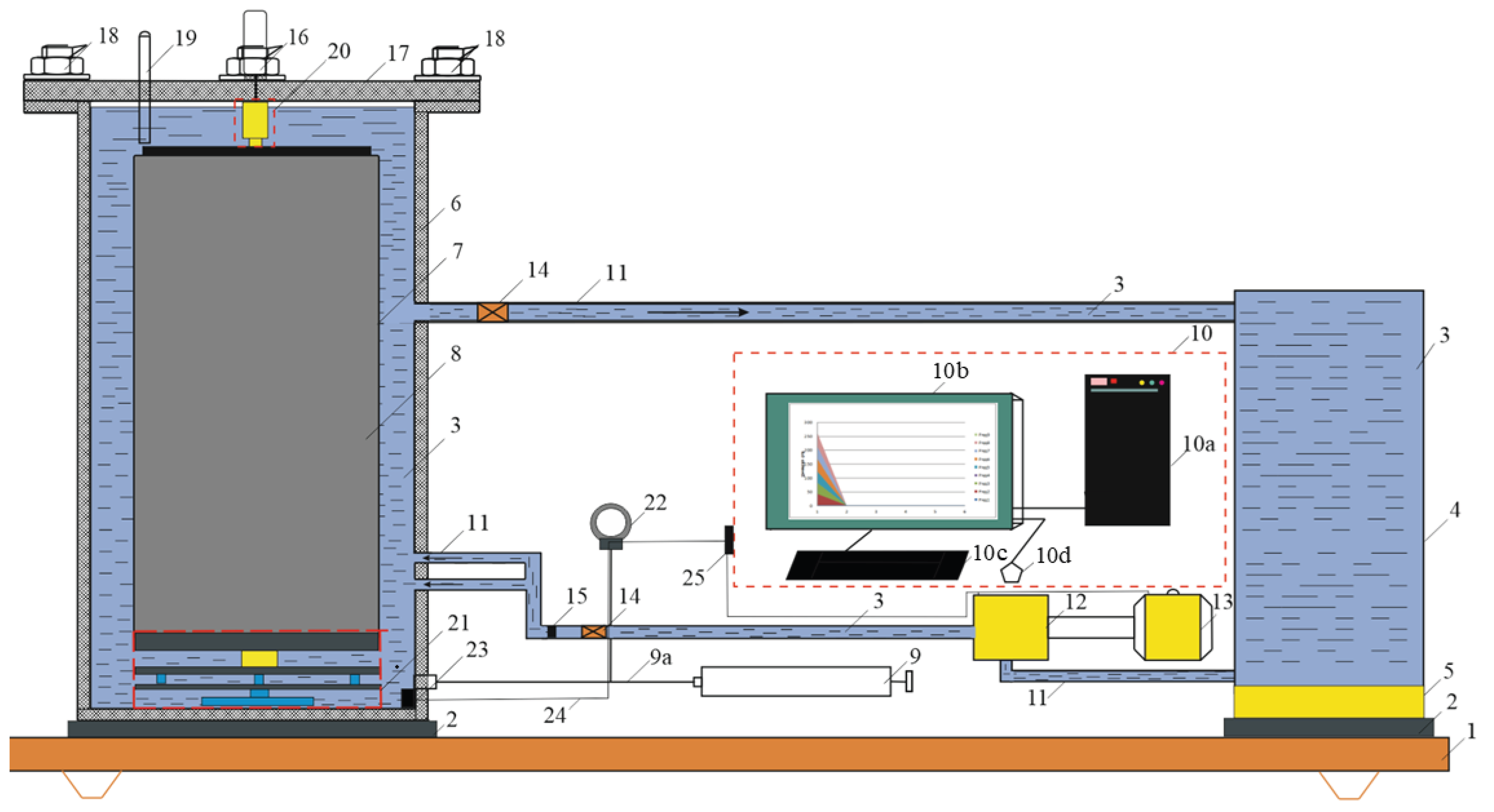
Figure 2.
Calculated profiles along the annulus for the example of Table 7: density (left), dynamic viscosity (centre) and bottomhole pressure (right). The dashed lines correspond to a calculation with constant surface values of density and viscosity.
Figure 2.
Calculated profiles along the annulus for the example of Table 7: density (left), dynamic viscosity (centre) and bottomhole pressure (right). The dashed lines correspond to a calculation with constant surface values of density and viscosity.
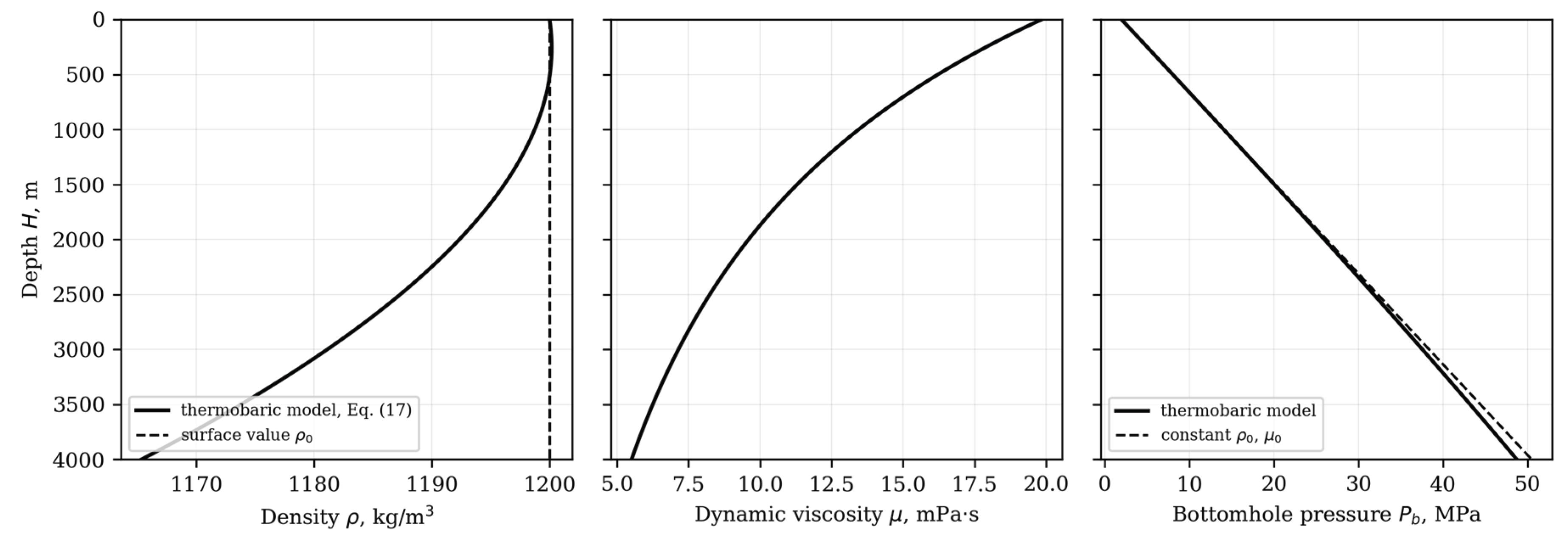
Table 1.
Thermal expansion coefficient (K⁻¹) for wellbore water.
| Pressure , MPa | Temperature interval , °C | ||||
|---|---|---|---|---|---|
| 1–10 | 10–20 | 40–50 | 60–70 | 90–100 | |
| 0.1 | 0.141 | 1.54 | 4.221 | 5.566 | 7.196 |
| 10 | 0.432 | 1.70 | 4.221 | 5.486 | 7.044 |
| 20 | 0.7201 | 1.86 | 4.262 | 5.393 | 6.881 |
| 50 | 1.492 | 2.39 | 4.292 | 5.232 | 6.615 |
Table 3.
Isothermal compressibility coefficient β (MPa⁻¹) expressed as reciprocal values.
| Temperature , °C | Pressure , MPa | ||||
|---|---|---|---|---|---|
| 0.5 | 1 | 2 | 4 | 8 | |
| 0 | 1/1888 | 1/1898 | 1/1915 | 1/1948 | 1/1978 |
| 5 | 1/1925 | 1/1945 | 1/1965 | 1/2012 | 1/2068 |
| 10 | 1/1949 | 1/1968 | 1/2008 | 1/2048 | 1/2118 |
| 15 | 1/1966 | 1/1998 | 1/2026 | 1/2093 | 1/2165 |
| 25 | 1/1975 | 1/2017 | 1/2054 | 1/2118 | 1/2215 |
Table 4.
Correlation coefficients for .
| , °C | rc | Assessment |
|---|---|---|
| 0 | -0.974 | NOT LINEAR |
| 5 | -0.99 | LINEAR |
| 10 | -0.9806 | NOT LINEAR |
| 15 | -0.9844 | NOT LINEAR |
| 25 | -0.9803 | NOT LINEAR |
Table 5.
Correlation coefficients for the isothermal bulk modulus versus pressure.
| , °C | rc | Assessment |
|---|---|---|
| 0 | 0.976 | NOT LINEAR |
| 5 | 0.992 | LINEAR |
| 10 | 0.985 | LINEAR |
| 15 | 0.988 | LINEAR |
| 25 | 0.986 | LINEAR |
Table 6.
Input parameters of the thermobaric model and methods of their determination.
| Parameter | Symbol, unit | Method of determination |
|---|---|---|
| Surface density | ρ0, kg/m³ | Hydrometer at (T0, P0) |
| Gradient of thermal expansion coefficient | gradα(T), K−2 | Least squares on α–T data, |r| ≥ 0.985 |
| Thermal expansion coefficient at surface | α(T0, P0), K−1 | Intercept of the α–T fit |
| Gradient of isothermal bulk modulus | grad(Eup), dimensionless | Least squares on Eup–P data, |r| ≥ 0.985 |
| Bulk modulus at surface | Eup(P0, T0), MPa | Intercept of the Eup–P fit |
| Frenkel–Andrade constants | A, Pa·s; E/k, K | Regression of ln μ on 1/T (≥3 temperatures) |
| Temperature gradient | m, K/m | Offset-well or downhole temperature data |
| Well and flow parameters | H, dh, v, P0 | Well design and drilling programme |
Table 7.
Input data of the worked example.
| Parameter | Value | Comment |
|---|---|---|
| ρ0 | 1200 kg/m³ | Polymer–bentonite fluid at 20 °C |
| T0 | 293.15 K (20 °C) | Surface temperature |
| P0 | 2.0 MPa | As in the example of Section 3.3 |
| m | 0.0225 K/m | Gives 110 °C at 4000 m, the upper test limit |
| H | 0–4000 m | As in the example of Section 3.3 |
| dh | 0.0889 m | 215.9 mm hole, 127 mm drill pipe |
| v | 1.2 m/s | As in the example of Section 3.3 |
| n = gradα(T) | 6.80 × 10⁻⁶ K−2 | Least-squares fit of Table 1, row P = 20 MPa |
| p = α(T0, P0) | −1.782 × 10⁻³ K−1 | Intercept of the same fit |
| q = grad(Eup) | 30.4 | Least-squares fit of Table 3, row T = 25 °C |
| r = Eup(P0, T0) | 1982 MPa | Intercept of the same fit |
| A | 8.46 × 10⁻⁵ Pa·s | Frenkel–Andrade constant, μ = 20 mPa·s at 20 °C |
| E/k | 1600 K | Frenkel–Andrade constant |
Table 8.
Calculated parameters of the drilling fluid along the annulus for the example of Table 7. ECD* is the equivalent circulating density referred to the hydrostatic and frictional components, i.e. (Pb − P0)/(gH).
Table 8.
Calculated parameters of the drilling fluid along the annulus for the example of Table 7. ECD* is the equivalent circulating density referred to the hydrostatic and frictional components, i.e. (Pb − P0)/(gH).
| H, m | T, °C | μ, mPa·s | ρ, kg/m³ | Re | ΔPf, MPa | Pb, MPa | ECD*, kg/m³ |
|---|---|---|---|---|---|---|---|
| 0 | 20.0 | 19.85 | 1200.0 | 6,450 | 0.00 | 2.00 | — |
| 500 | 31.2 | 16.22 | 1200.0 | 7,890 | 0.16 | 8.05 | 1233 |
| 1000 | 42.5 | 13.45 | 1198.7 | 9,510 | 0.31 | 14.07 | 1230 |
| 1500 | 53.8 | 11.30 | 1196.2 | 11,290 | 0.45 | 20.05 | 1226 |
| 2000 | 65.0 | 9.60 | 1192.4 | 13,250 | 0.57 | 25.96 | 1221 |
| 2500 | 76.2 | 8.24 | 1187.3 | 15,360 | 0.68 | 31.80 | 1215 |
| 3000 | 87.5 | 7.15 | 1181.1 | 17,630 | 0.79 | 37.55 | 1208 |
| 3500 | 98.8 | 6.25 | 1173.8 | 20,040 | 0.88 | 43.19 | 1200 |
| 4000 | 110.0 | 5.51 | 1165.4 | 22,570 | 0.97 | 48.70 | 1190 |
Disclaimer/Publisher’s Note: The statements, opinions and data contained in all publications are solely those of the individual author(s) and contributor(s) and not of MDPI and/or the editor(s). MDPI and/or the editor(s) disclaim responsibility for any injury to people or property resulting from any ideas, methods, instructions or products referred to in the content. |
© 2026 by the authors. Licensee MDPI, Basel, Switzerland. This article is an open access article distributed under the terms and conditions of the Creative Commons Attribution (CC BY) license.
Copyright: This open access article is published under a Creative Commons CC BY 4.0 license, which permit the free download, distribution, and reuse, provided that the author and preprint are cited in any reuse.