
Submitted:
01 October 2026
Posted:
13 October 2026
You are already at the latest version
Abstract
Here, we have shown that the temperature \((T)\) of an inert gas is proportional to \(w^{\frac{k_B}{nC_p}}\), where \(w\) is the number of microstates, \(n\) is the number of moles and \(C_p\) is the molar heat capacity at constant pressure and \(k_B\) is the Boltzmann constant. The above relationship has been found to be valid using experimental data in a wide range of temperature, e.g., \([298\,\mathrm{K}\text{--}6{,}000\,\mathrm{K}]\) for all the inert gases and we have documented their respective proportionality constants. On the other hand, for the non-inert gases, we have shown that the number of microstates is proportional to \[ T^{nA/k_B} \times e^{\frac{nBT}{1000k_B} + \frac{nCT^2}{2\times 1000^2\times k_B} + \frac{nDT^3}{3\times 1000^3\times k_B} - \frac{nE\times 1000^2}{T^2\times k_B}}, \] where \(A, B, C, D, E\) are coefficients of the Shomate equation for molar heat capacity at constant pressure. For three non-inert gases, namely, Hydrogen, Nitrogen and Oxygen, here we have estimated the values of the respective proportionality constants as well.
Keywords:
temperature
; microstates
; thermodynamics
; statistical mechanics
; inert gases
; non-inert gases
1. Introduction
Thermodynamics provides a macroscopic framework for describing the equilibrium properties and transformation of a physical system, while statistical mechanics strives to establish the microscopic foundation of these macroscopic laws. A central concept connecting these two disciplines is the number of accessible microscopic configurations of a system, otherwise known as state multiplicities, associated with a given macroscopic state. The statistical interpretation of entropy, expressed by the Boltzmann relation, , demonstrates that the state multiplicity w of a thermodynamic system is directly linked to its entropy S, thereby connecting thermodynamics with statistical mechanics [1]. On the other hand, temperature is one of the fundamental state variables in thermodynamics and the inverse of the temperature is conventionally defined as the partial derivative of the entropy of the system with respect to its internal energy, keeping volume (V) and the number of particles N constant [2]. Mathematically, . Moreover, in the canonical ensemble, temperature determines the statistical distribution of the system among its microscopic energy states, as described by the Boltzmann distribution [3,5]. In addition, in many statistical mechanics literature, temperature appears as a function of Lagrange Multiplier used to maximize state entropy [16]. Although the connection between temperature, entropy, and microscopic states is well established, a direct and general characterization of how the number of accessible microstates varies with temperature and the vice versa remain an important subject for quantitative analysis. In this work, we investigate the relationship between temperature and the number of accessible microstates in a gaseous closed system undergoing a reversible process due to application of heat. Starting from the statistical definition of entropy and the thermodynamic relation between entropy and temperature, we develop a novel thermodynamic framework, expressively connecting temperature and state multiplicities for ideal (inert) and non-ideal (non-inert) gases. To be precise, here we have shown that the temperature (T) of an inert gas is proportional to , where w is the number of microstates, n is the number of moles and is the molar heat capacity at constant pressure and is the Boltzmann constant. On the other hand, for the non-inert gases, we have shown that the number of microstates is proportional to , where are coefficients of the Shomate equation for molar heat capacity at constant pressure.
The rest of the article is organized as follows: Section 2 briefly describes the literature linking temperature with state multiplicities. Section 3 derives the relationship connecting temperature and state multiplicities for inert and non-inert gases. Section 4 explains the methodology used to measure the proportionality constants as derived in the previous section. Section 5 presents the results for 06 inert and 03 non-inert gases. Finally, section 6 concludes the article.
2. Literature Review: Temperature and the Number of Microstates
Statistical mechanics establishes a fundamental connection between the macroscopic quantity temperature (T) and the number of microscopic states (w) accessible to a system. The central concept underlying this connection is entropy, which, in the Boltzmann formulation, is related to the number of microscopic configurations compatible with the given macroscopic state of the system under consideration according to the following equation:
where S is the system entropy and is the Boltzmann constant. The logarithmic form of Eq. (1) is particularly useful as the multiplicities of statistically independent systems are multiplicative, whereas their thermodynamic entropies are additive. Thus, if two independent subsystems have multiplicities and , their combined multiplicity is , resulting in a consolidated entropy of [1,3,5].
The relationship between w and temperature follows directly from the thermodynamic definition of absolute temperature. For a simple closed system at fixed volume V and particle number N, the relationship can be described using the following equation:
where U is the internal energy of the system. Substituting the value of S from Eq. (1) into Eq. (2) results in the following equation:
Consequently, we can say that temperature of a system is not entirely determined simply by the absolute number of its accessible microstates, rather by the rate at which the logarithm of the number of accessible microstates changes with respect to the internal energy of the system, keeping the volume and constituent particles of the system constant. This distinction is important as two systems may have very different values of state multiplicities, while having the same temperature, provided their entropy-energy slopes are equal. Eq: (3) therefore provides a direct microscopic interpretation of temperature as being inversely proportional to the partial derivative of the logarithmic changes in state multiplicity with respect to internal energy of the system.
Moreover, in many statistical mechanics literature, temperature appears out of complex mathematical maneuvers without much physical significance/meaning [16]. For example, in the derivations of Boltzmann’s distribution law using Lagrange Multipliers to maximize system entropy, temperature emerges as the reciprocal of one of such multipliers namely, [18,20]. To be more precise, temperature is defined using the following equation:
Nelson (2019) provides a statistical mechanical interpretation of temperature arguing reciprocal of temperature corresponds to the relative change in the number of microscopic states accessible to a system, when its internal energy changes at fixed volume and composition [16]. This perspective is particularly useful because it complements the conventional presentation of temperature where temperature appears as the inverse of thermal parameter .
In addition, in the canonical ensemble, the probability of a microstate i with energy is defined as follows:
where Z is the canonical partition function. The temperature therefore controls how the statistical weight is distributed among microstates of different energy levels. At low temperatures, the Boltzmann factor strongly favors low-energy microstates, whereas increasing the temperature reduces the energetic bias and allows higher-energy microstates to acquire greater statistical weights [3,5,17]. In this sense, increasing temperature generally increases the set of energetically relevant microstates, although the precise relationship depends on the system’s energy spectrum and constraints.
Moreover, it is reported in the existing literature that the number of accessible energy microstates in a particulate system is temperature dependent and as the total energy of the system increases, as indicated by an increase in temperature or a change of state, the number of accessible energy microstates also increases [19]. For example, Tolley (2022) [19] relates temperature (T) with the number of microstates (W) in the following manner:
This result provides a quantitative route for connecting experimentally measurable thermal properties to the number of energetically accessible microstates. Tolley (2022) [19] specifically examined this connection, arguing heat-capacity measurements can be used to quantify the increase in energetic microstates and relating the temperature integral of heat capacity to the logarithm of the number of microstates. Their analysis is particularly relevant to approaches in which , rather than entropy alone, is treated as a fundamental quantity. The idea can be equivalently extended using molar heat capacity at constant pressure as well.
In summary, we can say that the existing literature reports that the number of accessible microstates increases monotonically with the increase in temperature. But there is no universally accepted proportional/inverse relationship between them. The literature also falls short of identifying any such proportional/inverse relationship between w and any well-defined function of temperature, i.e., as well or the vice versa.
3. Relating Temperature to Microstates
3.1. Inert Gases
Let us consider a closed system containing n moles of an inert gas undergoing a reversible process due to application of an infinitesimal amount of heat at constant pressure. Also, let the initial temperature be T. If the temperature of the system is changed by an amount due to application of heat, then the basic thermodynamic equation relating with is given by the following:
where is the molar heat capacity of the gas at constant pressure.
Moreover, the heat applied is supposed to bring about an infinitesimal change in entropy of the system. If the change in entropy is given by , then we have the following relation:
If we substitute the value of from the above equation into the first equation, we get:
Or equivalently,
Now consider, instead of applying infinitesimal amount of heat , we have applied amount of heat, which changes the temperature of the system from to and raises its entropy from to . So, integrating both sides of the above equation with respect to S and T, we get:
Or,
Moreover, if we substitute the thermodynamic definition of entropy, i.e., , where is the Boltzmann constant and w is the number of microstates, then we get:
Now, for inert gases, the molar heat capacity is temperature invariant and we can take it out of the integration sign and get:
Raising both sides to the power of e, we get:
The above relationship holds for any arbitrary final state of the system as well. For example, if we apply amount of heat to the system and the resulting final temperature and state multiplicity are given by and , then we can show that:
The above equation implies:
Or,
where is the proportionality constant.
3.2. Non-Inert Gases
Now consider a closed system containing n moles of a non-inert gas undergoing a reversible process due to application of an infinitesimal amount of heat at constant pressure. Also, let the initial temperature be T. If the temperature of the system is changed by an amount due to application of heat, then the basic thermodynamic equation relating with is given by the following:
Moreover, for any inert or non-inert gas, the following relationship holds:
Where is the change in entropy of the system due to application of heat . From the above two equations, we can get:
Now, instead of applying infinitesimal amount of heat , we consider applying amount of heat into the system, resulting into a change in entropy from to and a change in temperature from to . So, integrating both sides of the above equation yields:
Or,
Substituting the value of and from Boltzmann’s equation, yields:
At this stage, the derivation diverges from that of an inert gas. For any non-inert gas, the value of molar heat capacity at constant pressure does not usually remain constant over the entire temperature range. Rather, it varies with temperature and thus we cannot simply take it out the integration sign. Instead, we use Shomate equation to approximate at different temperatures. Shomate equations are empirical polynomial formulations used to approximate heat capacity, enthalpy, and entropy of different chemical substances across varying temperatures [4]. For molar heat capacity at constant pressure, Shomate equation can be written as follows:
where . Now, substituting the value of from the above equation into equation 13, yields:
Raising both sides to the power of e, we obtain:
So,
Or,
where
The above relationship holds for any arbitrary final state of the system as well. For example, if we apply an amount of heat to the system and the resulting final temperature and state multiplicity are given by and respectively, then we can show that:
The above equation implies:
Or,
where is the proportionality constant.
The above equation implies:
Substituting the value of w from Boltzmann equation into the above, yields:
Simplifying the above, we get:
Denoting by Q for convenience, we get:
Taking logarithm on both sides of the above equation, we get:
So, after simplification, the logarithm of the proportionality constant is given by the following:
4. Methodology
We collect molar heat capacity and entropy data at different temperatures for all the inert gases, i.e., Helium, Neon, Argon, Krypton, Xenon, Radon and 03 non-inert gases, namely, Hydrogen, Nitrogen and Oxygen from NIST Chemistry Web Book [6]. We use equation 11 to estimate the values of for all the inert gases in the temperature range K. Moreover, we use Boltzmann equation to determine the value of state multiplicities w at different temperatures. On the other hand, to determine the value , we use equation 20. To estimate , we first need to determine the value of Q and A, where A is the first coefficient of the respective Shomate equation for molar heat capacity at constant pressure. In addition, to determine Q, we need to have the values of all the coefficients, i.e., of Shomate equation [4]. It is to be noted in this regard that the values of the coefficients do not remain constant for the non-inert gases in different temperature ranges. For example, for Hydrogen NIST Chemistry Web Book reports 3 sets of values for the coefficients in different temperature ranges: For temperature range K, K and K, the values of are reported to be [33.066178, -11.363417, 11.432816, -2.772874, -0.158558], [18.563083, 12.257357, -2.859786, 0.268238, 1.977990] and [43.413560, -4.293079, 1.272428, -0.096876, -20.533862] respectively. We use appropriate values of the coefficients depending upon the temperature range under consideration.
5. Results
5.1. Inert Gases
In this subsection, we are going to report the estimated value of the proportionality constant as defined in equation 11 for all the 06 inert gases, namely, Helium, Neon, Argon, Krypton, Xenon and Radon in the temperature range K.
5.1.1. Helium
We use equation 11 to estimate the proportionality constant for Helium. To use equation 11, we first need to estimate the value of state multiplicity w and we do so by rearranging the Boltzmann equation into the form , where S is the state entropy and is the Boltzmann constant. We collect the value of state entropy of 1.0 mole of Helium and molar heat capacity at constant pressure from gas phase thermochemistry data for Helium from NIST Chemistry Web Book [8]. It is to be noted in this regard that the molar heat capacity at constant pressure for Helium is and it is constant throughout the temperature range K. On the other hand, the state entropy of 1.0 mole of Helium is reported to be at 298 K, which gradually rises to at 6,000 K at standard pressure. Substituting the value of w and into equation 11 yields the value of the proportionality constant in the temperature range K. The estimated value of the proportionality constant is found to be , which effectively remains constant in the entire temperature range under consideration. This is graphically shown in Figure 1.
5.1.2. Neon
Like before, we collect state entropy data of 1.0 mole of Neon at standard pressure in the temperature range K and molar heat capacity at constant pressure from gas phase thermochemistry data for Neon [10]. It is found that the molar heat capacity of Neon at standard pressure is constant at in the temperature range K. On the other hand, the entropy of 1.0 mole of Neon at standard pressure is found to be at 298 K, which gradually rises to at 6,000 K. Substituting the value of w (as calculated from ) and into equation 11, we get the respective proportionality constant for Neon. The value of is estimated to be 0.26 in the entire temperature range K. This is graphically shown in Figure 2.
5.1.3. Argon
We collect molar heat capacity at constant pressure (standard pressure) and state entropy data of 1.0 mole of Argon in the temperature range K from gas phase thermochemistry data for Argon [7]. Like all other inert gases, the molar heat capacity for Argon at standard pressure remains constant at . On the other hand, the state entropy of 1.0 mole of Argon at 298 K temperature and standard pressure is found to be , which gradually rises to at K and standard pressure. Once we have the values of S and , we can use equation 11 to measure the proportionality constant . The value of is measured to be 0.17 for Argon in the temperature range K. This is graphically shown in Figure 3.
5.1.4. Krypton
Like all other inert gases, molar heat capacity at constant pressure of Krypton at standard pressure is found to be constant at [9]. Moreover, the state entropy of 1.0 mole of Krypton varies between at standard pressure in the temperature range K [9]. Using the values of and S, we can estimate the proportionality constant for Krypton and it is found to be 0.11. This is graphically shown in Figure 4.
5.1.5. Xenon
Molar heat capacity at constant standard pressure of Xenon is [14]. In addition, the entropy of 1.0 mole of Xenon at constant standard pressure is found to vary between in the temperature range K. Substituting these values into equation equation 11, we can estimate the value of for Xenon in different temperature range. The estimated value of is found to be 0.085 and this is graphically shown in Figure 5.
5.1.6. Radon
We collect state entropy of 1.0 mole of Radon at standard pressure and in different temperatures from gas phase thermochemistry data for Radon [13]. Moreover, like all other inert gases, the molar heat capacity at constant standard pressure for Radon is constant at [13]. Using the values of entropy and molar heat capacity at constant pressure, we can estimate the respective proportionality constant for Radon in different temperature range. The value of for Radon is estimated to be 0.062 and it effectively remains constant throughout the temperature range K. The results are graphically shown in Figure 6.
5.2. Non-Inert Gases
In the previous subsection, we have estimated and reported the proportionality constant for all the inert gases in the temperature range K. In this subsection, we are going to report the experimental values of the logarithm of the proportionality constant as defined in equation 20 for three non-inert gases, namely, Hydrogen, Nitrogen and Oxygen.
5.2.1. Hydrogen
For Hydrogen, we collect molar heat capacity data at constant standard pressure in the temperature range K from NIST Chemistry Web Book page for Hydrogen [15]. From the data, it is observed that unlike the inert gases, the molar heat capacity of Hydrogen at constant pressure varies with temperature, starting at 28.84 at 298 K and gradually rising to 41.97 at 6,000 K. It is to be noted in this regard that Shomate equation for molar heat capacity at constant pressure () introduces an empirical polynomial equation relating to temperature with the help of five coefficients and E. The values of and E do not remain constant throughout the temperature range [4]. For Hydrogen, the values of the coefficients are reported to be [33.066178, -11.363417, 11.432816, -2.772874, -0.158558], [18.563083, 12.257357, -2.859786, 0.268238, 1.977990] and [43.413560, -4.293079, 1.272428, -0.096876, -20.533862] respectively in the temperature range K, K and K. We use the appropriate values of these coefficients, when estimating the values of in different temperatures. On the other hand, state entropy of 1.0 mole of Hydrogen changes from 130.70 at 298 K to 230.30 at 6,000 K [15]. Now, as we have the values of S and the values of the coefficients , we can use equation 20 to approximate the values of in different temperatures. The results are depicted in Figure 7.
From Figure 7, we can see that the value of for Hydrogen does not remain constant in the entire temperature range of K. Rather, the values vary in three distinct levels corresponding to three different sets of values of the coefficients of the Shomate equation. For the temperature range K, K and K, the value of is found to be , and respectively.
5.2.2. Nitrogen
We collect state entropy and molar heat capacity () data at constant standard pressure for Nitrogen from NIST Chemistry Web Book page for Nitrogen [11]. Like Hydrogen and all other real gases, does not remain constant in the temperature range K. Rather, it varies between 29.10 at 100 K to 38.27 at 6,000 K. State entropy of 1.0 mole Nitrogen is found to fluctuate between 159.80 at 100 K and 293 at 6,000 K. Moreover, Shomate equation for for Nitrogen reports three sets of values for the coefficients and E. The reported values of and E are found to be [28.98641, 1.853978, -9.647459, 16.63537, 0.000117], [19.50583, 19.88705, -8.598535, 1.369784, 0.527601] and [35.51872, 1.128728, -0.196103, 0.014662, -4.55376] respectively in the temperature range [100-500] K, [500-2,000] K and [2,000-6,000] K. Once we substitute the values of and into equation 20, we get the values of in the temperature range [100-6,000] K. The results are graphically presented in Figure 8.
From Figure 8, we can see that the value of varies with temperature. Like Hydrogen, the graph of looks like a step function, where each step corresponds to each set of values of the coefficients of the Shomate equation. In the temperature range of [100-500] K, [500-2,000] K and [2,000-6,000] K, the value of is found to be , and respectively.
5.2.3. Oxygen
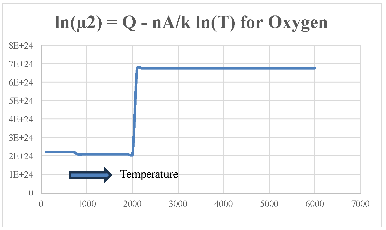
From NIST Chemistry Web Book page for Oxygen [12], it has been observed that molar heat capacity at constant standard pressure for Oxygen varies between 29.10 at 100 K and 44.39 at 6,000 K. Moreover, state entropy of 1.0 mole of Oxygen is 173.30 at 100 K, which rises gradually to 313.50 at 6,000 K. Moreover, the values of the coefficients of the Shomate equation are reported to be , and respectively in the temperature range , and . Substituting the values of S and into equation 20, we get the values of in the temperature range [100-6,000] K. The results are graphically presented in Figure 9.
6. Conclusion
In this study, we have established new relationships between state multiplicity (w), a statistical mechanical quantity and temperature (T), a thermodynamic variable for both inert and non-inert gases. To be more precise, here we have shown that for inert gases, the temperature is proportional to and for non-inert gases, state multiplicity is proportional to . We have explicitly determined the function and and also measured the respective proportionality constants by drawing insights from both thermodynamics and statistical mechanics. The objective of this study is therefore not merely to reinterpret the established entropy-microstate nexus, but to formulate and analyze a temperature-dependent relationship that can provide an explicit bridge between a measurable thermodynamic variable and the state multiplicity of the system. Such a relationship may offer an alternative perspective on the statistical interpretation of thermal processes and provide a basis for further investigation of more complex gaseous and many-particle systems.
Funding
No funding is received to accomplish this work.
Conflicts of Interest
Author of the paper declares that he has no conflict of interest regarding this article. No human participation or animal trial is involved.
References
- Boltzmann, Ludwig. On the relation between the second law of the mechanical theory of heat and the probability calculus, or the theorems on thermal equilibrium. Proc. Imp. Acad. Sci. 1877, 76, 373–435. [Google Scholar]
- Callen, Herbert B. Thermodynamics and an Introduction to Thermostatistics, 2 edition; John Wiley & Sons: New York, 1985. [Google Scholar]
- Callen, Herbert B. Thermodynamics and an Introduction to Thermostatistics, 2 edition; John Wiley & Sons: New York, 1985. [Google Scholar]
- Chase, Jr. Malcolm W. NIST-JANAF Thermochemical Tables. In Journal of Physical and Chemical Reference Data, Monograph 9, 4 edition; American Chemical Society and American Institute of Physics: New York, 1998. [Google Scholar]
- Gibbs, J. Willard. Elementary Principles in Statistical Mechanics; Charles Scribner’s Sons: New York, 1902. [Google Scholar]
- National Institute of Standards and Technology. Nist chemistry webbook. Available online: https://webbook.nist.gov/chemistry/ (accessed on 2026-09-29).
- National Institute of Standards and Technology. Nist chemistry webbook: Argon. In NIST Standard Reference Database 69.
- National Institute of Standards and Technology. Nist chemistry webbook: Helium. In NIST Standard Reference Database 69.
- National Institute of Standards and Technology. Nist chemistry webbook: Krypton. NIST Stand. Ref. Database 69. [CrossRef]
- National Institute of Standards and Technology. Nist chemistry webbook: Neon. NIST Stand. Ref. Database 69. [CrossRef]
- National Institute of Standards and Technology. Nist chemistry webbook: Nitrogen. In NIST Standard Reference Database 69.
- National Institute of Standards and Technology. Nist chemistry webbook: Oxygen. In NIST Standard Reference Database 69.
- National Institute of Standards and Technology. Nist chemistry webbook: Radon. NIST Stand. Ref. Database 69. [CrossRef]
- National Institute of Standards and Technology. Nist chemistry webbook: Xenon. NIST Stand. Ref. Database 69. [CrossRef]
- National Institute of Standards and Technology. Nist chemistry webbook: Hydrogen, 2026. In NIST Standard Reference Database 69.
- Nelson, Peter G. Statistical mechanical interpretation of temperature. Found. Chem. 2019, 21(3), 325–331. [Google Scholar] [CrossRef]
- Reif, Frederick. Fundamentals of Statistical and Thermal Physics; McGraw-Hill: New York, 1965. [Google Scholar]
- Schrödinger, Erwin. Statistical Thermodynamics: A Course of Seminar Lectures; Cambridge University Press: Cambridge, 1946. [Google Scholar]
- Tolley, H. Dennis; Woodfield, Brian F.; Hansen, Lee D. Counting microstates via heat capacity and implications for the third law. J. Chem. Thermodyn. 2022, 171, 106807. [Google Scholar] [CrossRef]
- Tolman, Richard Chace. The principles of statistical mechanics; Courier Corporation, 1979. [Google Scholar]
Figure 1.
Value of the proportionality constant for Helium
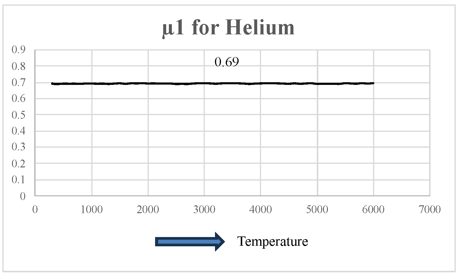
Figure 2.
Value of the proportionality constant for Neon
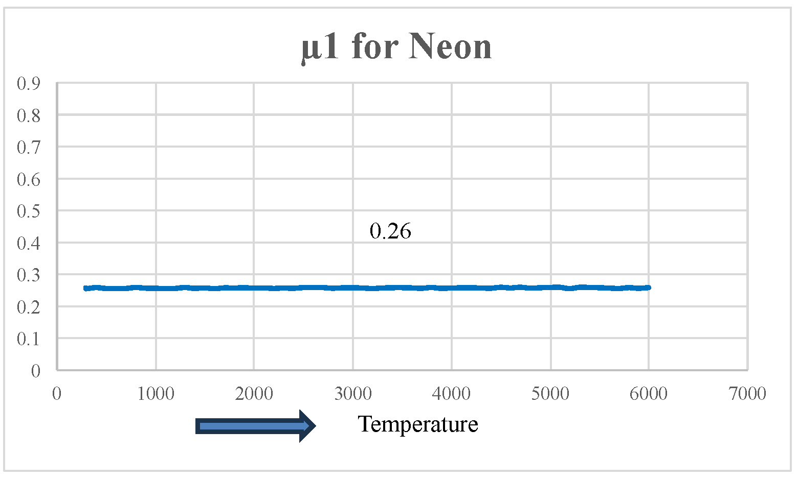
Figure 3.
Value of the proportionality constant for Argon
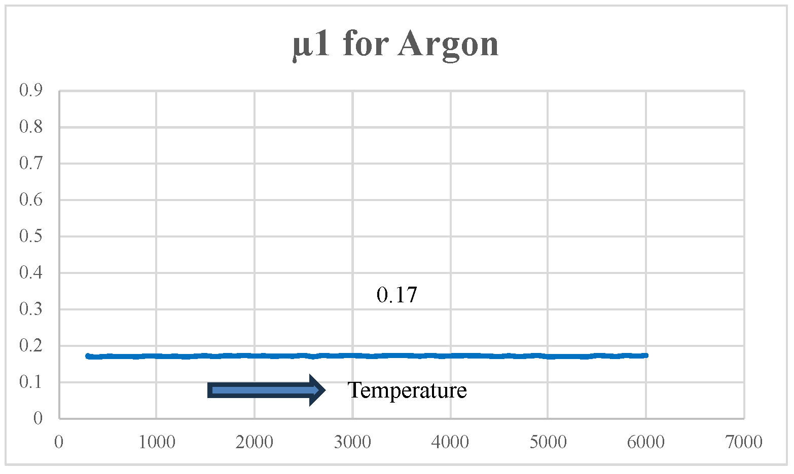
Figure 4.
Value of the proportionality constant for Krypton
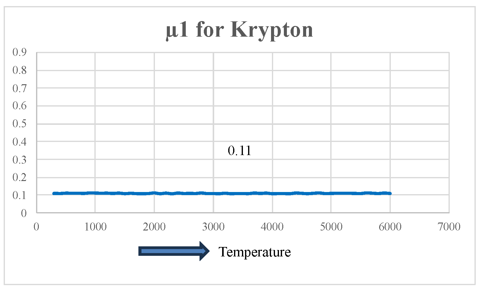
Figure 5.
Value of the proportionality constant for Xenon
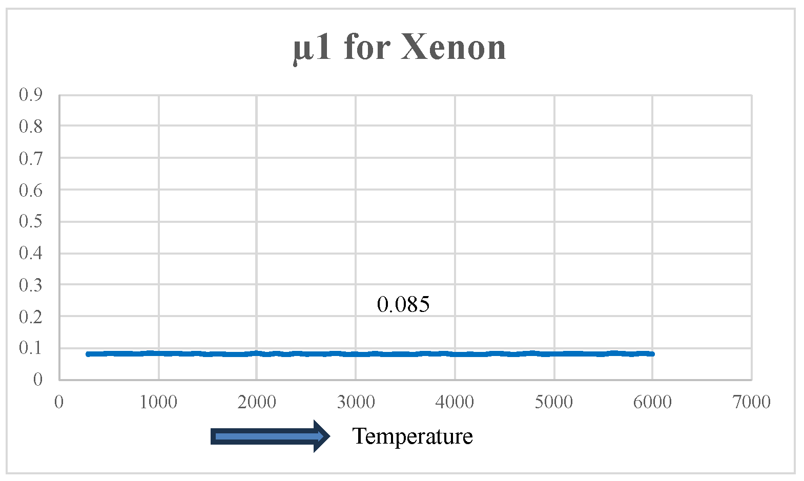
Figure 6.
Value of the proportionality constant for Radon
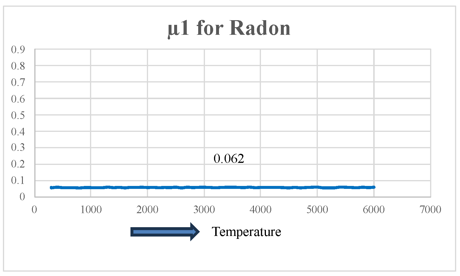
Figure 7.
Value of the logarithm of the proportionality constant () for Hydrogen
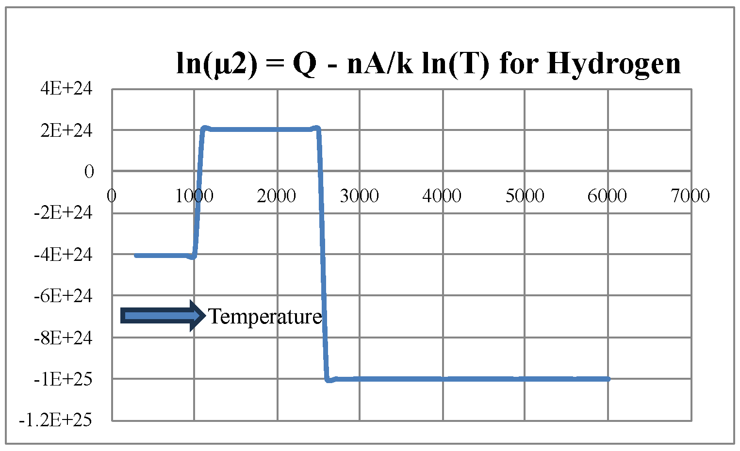
Figure 8.
Value of the logarithm of the proportionality constant () for Nitrogen
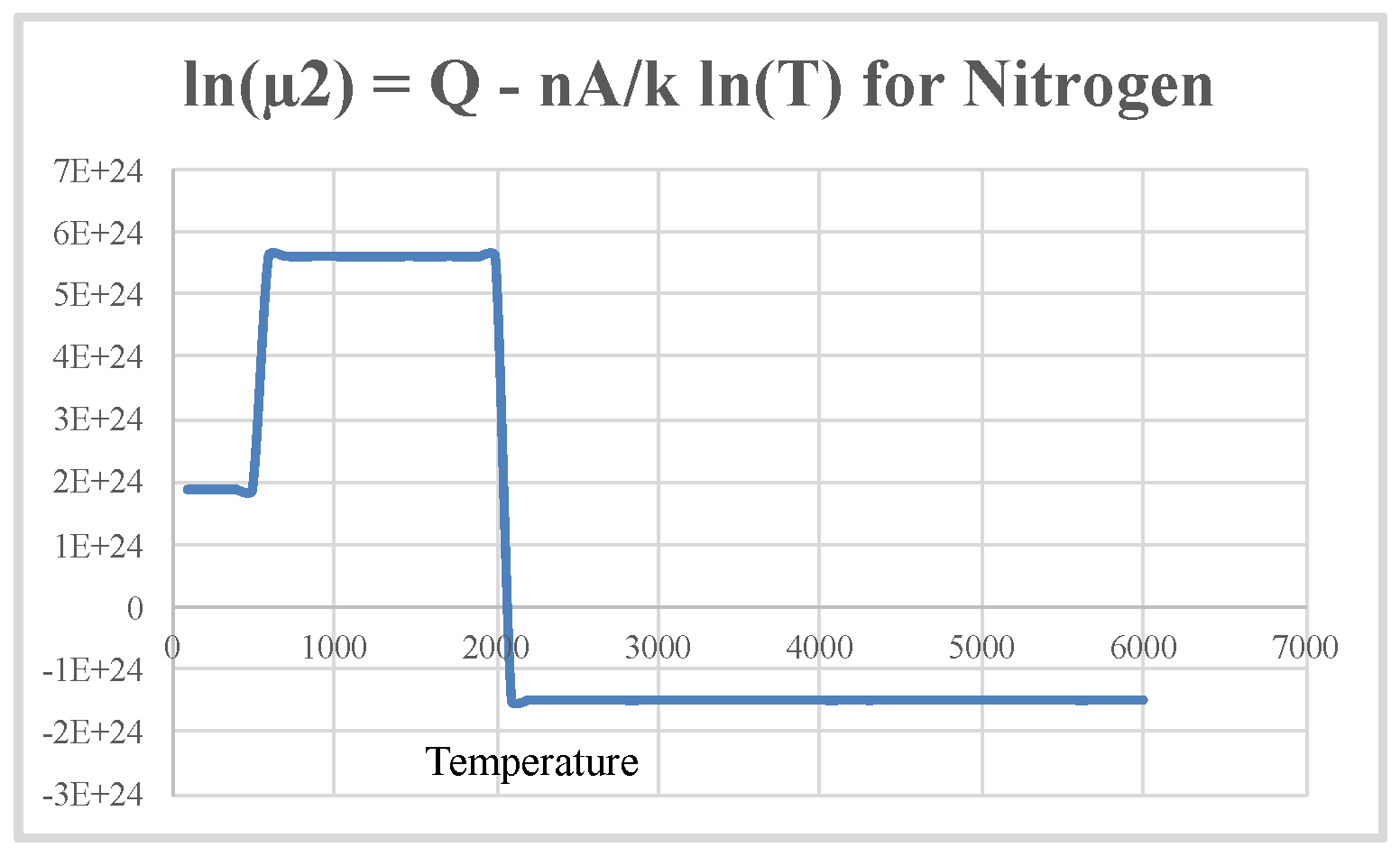
Figure 9.
Value of the logarithm of the proportionality constant () for Oxygen
Disclaimer/Publisher’s Note: The statements, opinions and data contained in all publications are solely those of the individual author(s) and contributor(s) and not of MDPI and/or the editor(s). MDPI and/or the editor(s) disclaim responsibility for any injury to people or property resulting from any ideas, methods, instructions or products referred to in the content. |
© 2026 by the authors. Licensee MDPI, Basel, Switzerland. This article is an open access article distributed under the terms and conditions of the Creative Commons Attribution (CC BY) license (http://creativecommons.org/licenses/by/4.0/).
Copyright: This open access article is published under a Creative Commons CC BY 4.0 license, which permit the free download, distribution, and reuse, provided that the author and preprint are cited in any reuse.