

Submitted:
10 October 2026
Posted:
12 October 2026
You are already at the latest version
Abstract
This work investigates the link between surface topography at the mesoscopic scale and emissivity at the macroscopic scale within the Morphology-Driven Radiative Analysis and Design framework. The analysis is conducted on periodic lamellar titanium gratings characterized by the period P, groove width W, and groove depth H. Their emissivity is investigated by comparing three modelling approaches: the Agababov model, ray-tracing simulations, and Rigorous Coupled-Wave Analysis (RCWA), used as the electromagnetic reference. A numerical design comprising 8,100 configurations is used to investigate the effects of geometry, wavelength, and incidence angle. The results show that the accuracy of the geometrical-optics models (Agababov and ray tracing) is governed by the relative scales of the surface geometry and wavelength, as well as by the incidence angle. The largest discrepancies with respect to the electromagnetic solution occur at small P/λ, particularly when associated with large H/λ. The resulting validity regions and their dependence on incidence angle are consistent with the trends reported by Tang and Fu. Overall, ray tracing does not systematically outperform the Agababov model, which exhibits errors of the same order over substantial regions of the investigated parameter space, highlighting its ability to provide reliable predictions despite its simpler formulation.
Keywords:
surface roughness
; emissivity
; Agababov’s model
; ray tracing
; rigorous coupled wave analysis
; titanium
1. Introduction
Emissivity is a key surface property in radiative heat transfer and is required in a wide range of applications. It governs, for instance, the radiative heat rejection of spacecraft [1], contributes to the passive thermal management of electronic enclosures [2], enters the design of solar absorbers and selective coatings [3], and is a critical parameter in non-contact temperature measurements by radiation thermometry [4]. For real surfaces, emissivity cannot be regarded as an intrinsic material constant. In addition to wavelength, temperature and incident/measurement angle, it depends strongly on the surface state, particularly on surface roughness and oxidation [5,6].
This dependence has motivated numerous studies in which the surface state is modified to control radiative properties. A representative example is the work of [2], who combined sandblasting and chemical etching to create a multiscale rough structure on an aluminium alloy intended for outdoor electronic enclosures. The resulting surface exhibited an infrared emissivity of approximately 0.90 and improved radiative heat dissipation, leading to a reduction of the enclosure internal temperature. Such results illustrate that surface morphology can constitute a direct engineering lever for modifying the radiative response of a component.
The present work is part of a broader Morphology-Driven Radiative Analysis and Design (MORPHORAD) framework, which aims at relating surface morphology to observed radiative properties through physical modelling, experimental measurements and an explicit description of the relevant scales of analysis. Four scales are distinguished, as illustrated in Figure 1. The system scale corresponds to the component in its operating environment. The macro scale refers to the region of interest in which the radiative property is observed or measured under controlled conditions. The meso scale describes the actual surface geometry, including topography, roughness and texture. Finally, the micro scale accounts for the intrinsic properties of the material, including its composition and electronic structure, from which its optical properties and the underlying wave–matter interactions originate.
This work focuses on the link between the meso and macro scales, namely the prediction of macroscopic emissivity from the geometry of the surface. The system scale is therefore left outside the present scope. The micro scale, however, remains necessary because it provides the optical properties entering the surface–radiation interaction. To make the link between the meso and the macro scale, several models have been proposed in the literature, and they may first be classified according to the physics they assume. A first class relies on geometrical optics. In this description, the characteristic dimensions of the surface are sufficiently large compared to the wavelength. Here, phenomena associated with the wave nature of electromagnetic radiation, such as diffraction and interference, are neglected. The validity of this approximation therefore depends on dimensionless ratios involving the characteristic dimensions of the surface and the wavelength, as well as on the incidence angle [7,8,9]. Conversely, when surface dimensions become comparable with the wavelength, wave effects become significant and the electromagnetic nature of the problem must be explicitly accounted for.
Within the geometrical-optics class, the Agababov’s model constitutes one of the simplest reduced descriptions of the roughness effect. Agababov represented a rough surface as an assembly of geometrical depressions and related its effective emissivity to that of a smoother reference surface through a roughness factor [10,11]. The resulting formulation is explicit and computationally inexpensive because the detailed interaction of the radiation with the complete surface does not need to be resolved.
[12] subsequently applied this approach to model the influence of roughness on the emissivity of aluminium alloys. [13] modified the Agababov roughness function to predict the normal spectral emissivity of roughened cobalt, while [14] extended this type of approach by constructing random rough surfaces and evaluated it on several engineering alloys, including GH3044, K465, DD6 and TC4. These studies illustrate the attractiveness of the Agababov’s model for rapidly estimating roughness-induced changes in emissivity.
A more detailed geometrical-optics description is provided by ray tracing. Instead of reducing the topography to a single roughness factor, ray tracing explicitly follows radiation trajectories over the surface. At each interaction, the local incidence angle and reflection coefficient can be evaluated, while shadowing and successive reflections inside surface cavities can naturally be taken into account. This approach has been used extensively to investigate radiative interactions with rough surfaces. [15], for example, used ray tracing to study the absorptivity of micro-rough periodic surfaces and compared its predictions with a wave-based calculation. [16] employed three-dimensional ray tracing to investigate the absorption of light by rough metallic surfaces, with direct relevance to laser–material interactions. Lin used the ray tracing to interpret the spectral radiative properties of advanced high-strength steels from measured surface topographies [17].
Both the Agababov’s model and ray tracing nevertheless remain approximations of the electromagnetic interaction. Their underlying geometrical-optics assumptions progressively lose validity when the characteristic dimensions of the surface approach the wavelength, because phase, interference and diffraction can no longer be neglected. In this regime, the electromagnetic field must be explicitly resolved from Maxwell’s equations. Numerical methods such as the Finite-Difference Time-Domain method (FDTD) [18] and Rigorous Coupled-Wave Analysis (RCWA) [19] provide such a description. RCWA is particularly suited to periodic structures and has also been successfully applied to experimentally measured rough profiles. Sainz-Menchón, for example, showed that RCWA can reproduce the directional spectral emissivity of rolled aluminium while accounting for its multiscale surface roughness [6]. The greater physical completeness of these methods, however, comes at a substantially higher computational cost than geometrical-optics models.
The transition between geometrical-optics and electromagnetic descriptions has been investigated in several studies. Tang compared geometrical-optics predictions with rigorous electromagnetic scattering calculations over broad ranges of roughness, correlation length, wavelength and incidence angle, and established regions of validity for the geometrical-optics approximation [7]. Their analysis was subsequently extended to two-dimensional random rough surfaces [8], while [9] proposed an updated regime map from comparisons between geometrical optics and FDTD calculations . These works provide important criteria for the applicability of geometrical optics. However, these criteria are primarily formulated for numerically generated random rough surfaces. Such surfaces lend themselves particularly well to statistical studies, but their exact reproduction for experimental validation remains a challenge. Furthermore, to conduct such a study rigorously, a sensitivity analysis focused on the choice of roughness parameters and their numerical estimation scale is necessary.
The present work addresses this point using periodic lamellar titanium gratings, selected because their characteristic dimensions can be independently controlled numerically and because the corresponding geometry can, in principle, be reproduced experimentally. Three modelling levels are considered: the Agababov’s model, the ray tracing and the RCWA. Using the RCWA electromagnetic solution as a reference, the study first examines the sensitivity of emissivity to the characteristic dimensions of the generated surface, their relationship to wavelength and the angle of incidence. It then quantifies how the errors associated with Agababov and ray tracing approaches vary across the parameter space. In addition to this aspect, one of the objectives is also to evaluate whether Agababov’s model provides a sufficiently accurate and robust representation of the variations in emissivity induced by roughness, and to identify the conditions under which a more detailed geometric or electromagnetic description becomes necessary.
2. Modelling and Methodology
2.1. Emissivity of an Opaque Surface
For an opaque material, as we assumed for titanium, transmission is neglected and energy conservation gives (Equation (1)):
where is the spectral directional absorptance, is the spectral directional reflectance, is the wavelength, is the zenith angle of incidence measured with respect to the surface normal, and is the azimuthal angle of incidence. At thermal equilibrium (T), Kirchhoff’s law [20] states that the emissivity equals the absorptance:
Thus, for an opaque surface, we have :
2.2. Optical Properties of the Material
For a smooth planar interface, the reflected and transmitted fields are described by the Fresnel relations [21], and formulated within the framework of classical electromagnetism by [22,23]. The incident electromagnetic wave can be decomposed into two independent polarization states: transverse electric (TE), or s-polarization, and transverse magnetic (TM), or p-polarization. For TE polarization, the electric field is perpendicular to the plane of incidence, while the magnetic field lies within this plane. Conversely, for TM polarization, the magnetic field is perpendicular to the plane of incidence, while the electric field lies within it, as illustrated in Figure 2.
For incidence from air onto an absorbing medium characterized by the complex refractive index , where n is the refractive index and k is the extinction coefficient, the Fresnel reflectances associated with the TE and TM polarizations are given by :
where and are the complex amplitude reflection coefficients for s- and p-polarized waves, respectively given by :
For incidence from air, the corresponding refraction angle is related to the incidence angle through Snell–Descartes’s law :
For unpolarized radiation, assumed to contain equal contributions from the two orthogonal polarization states, the Fresnel reflectance is obtained by averaging the TE and TM contributions:
The complex refractive index of titanium is taken from Rakić et al. [24], using their Lorentz–Drude representation.
2.3. Geometry and Its Parameters
The textured surface consists of a periodic rectangular groove geometry characterized by the period P, the ridge width W and the groove depth H, as illustrated in Figure 3.
Periodic lamellar gratings were selected because their geometry can be fully described by a limited number of independently controlled parameters, enabling investigation of the influence of surface geometry on radiative properties. Their periodicity also makes them well suited to an electromagnetic treatment by Rigorous Coupled Wave Analysis tool. From an experimental perspective, rectangular periodic textures also offer the advantage of being fabricated with a high degree of reproducibility, and can therefore be targeted in future experimental validation campaigns using controlled manufacturing techniques such as laser texturing.
2.4. Models Studied
2.4.1. Agababov’s Model
A simple and computationally inexpensive way to introduce the effect of surface roughness into a radiative model is the relation of Agababov [25], which relates the effective emissivity of a rough surface to that of the corresponding smooth surface through a geometric roughness factor R :
where denotes the emissivity of the smooth reference surface. The roughness factor is expressed in terms of the increase in developed surface area, following an approach inspired by the work of [26]. This geometrical contribution is quantified using the ISO 25178 [27] areal parameter , i.e., the developed interfacial area ratio, which represents the percentage increase in the developed area of the topographic surface relative to its projected area. The roughness factor is therefore written as :
For the ideal rectangular lamellar geometry considered here, the developed surface area over one period, per unit length along the grooves, is , whereas the corresponding projected area is P. The geometric roughness factor therefore becomes
and the Agababov relation can be written as
For a given smooth-surface emissivity , this formulation depends on the depth-to-period ratio , but contains no explicit dependence on the ridge width W or the filling fraction . Consequently, it predicts the same emissivity for structures with identical P and H but different ridge widths, although their groove openings differ. This is an intrinsic limitation of the area-based formulation used in this study: reducing the morphology to a single developed-area factor does not retain the geometric information required to distinguish opening-dependent reflection and escape paths. Such effects cannot therefore be expected to be captured by this formulation.
2.4.2. Ray Tracing
Each ray is initialized at a position located above the highest point of the surface and sampled over the projected domain. The initial propagation direction is defined by
where is the polar incidence angle measured from the macroscopic surface normal and is the azimuthal angle measured in the plane. The ray energy is updated at each successive interaction. If denotes the energy carried by the ray immediately before impact j, the absorbed energy and the remaining reflected energy are given by :
where and denote the local absorptance and local Fresnel reflectance at impact j. The total energy absorbed along the trajectory of ray q is :
where is the number of surface interactions experienced by ray q. The effective absorptance estimated from incident rays is given by :
and the effective emissivity predicted by ray tracing follows from Kirchhoff’s law :
The main numerical parameters used for the ray-tracing simulations are summarized in Table 1, and their selection is justified in Section 2.5.
2.4.3. Electromagnetic Reference: Rigorous Coupled Wave Analysis (RCWA)
RCWA is the electromagnetic method used as the reference. The geometry considered is invariant along the y direction, so that the electromagnetic problem is two dimensional and is solved with a 2D RCWA formulation. Assuming harmonic fields, Maxwell’s curl equations are written as :
where and are the electric and magnetic fields, is the angular frequency, and are the vacuum permittivity and permeability, and is the relative permittivity distribution describing the periodic structure. The relative permittivity and the electromagnetic fields are expanded into a finite number of spatial Fourier harmonics along the periodic direction x :
where m is the diffraction order index, is the corresponding reciprocal lattice vector, is the mth Fourier coefficient of the permittivity distribution, and is the total number of retained harmonics. The electric field is expanded in the same basis as :
where denotes the amplitude associated with the mth diffraction order and is the x component of the incident wave vector, so that the tangential wave vector component of order m is . Substituting Equations 18 and 19 into Equation 17 transforms the problem into a system of coupled equations, which is solved order by order in TE and TM. The number of retained harmonics controls the accuracy of the Fourier representation: is the value used, as justified in Section 2.5.
2.5. Convergence Study
The main numerical parameters of the ray-tracing and RCWA solvers were selected from a convergence study. The results are reported in Figure 4.
The estimated emissivity increases with the number of launched rays and reaches a plateau beyond about rays (Figure 4(a)), the value retained, , therefore lying two orders of magnitude inside the converged region. Figure 4(b) shows the dependence on the maximum number of reflections. As a precaution, a large value, , is retained. This choice does not increase the computational cost, since the process can also be terminated earlier when the energy criterion is satisfied. In Figure 4(c), emissivity is insensitive to the energy termination threshold as long as it remains below about , so is a conservative choice. Finally, the emissivity decreases markedly as the number of harmonics increases and stabilizes beyond a few hundred harmonics (Figure 4(d)). The value is therefore a reasonable choice.
2.6. Validation Against Another Solver
Since the reference solution is developed in-house, its predictions is compared with another solver. The comparison is performed with Ansys Lumerical using its finite-difference time-domain (FDTD) solver, which discretizes Maxwell’s curl equations directly in space and time on a staggered grid [28] and therefore shares no formulation with the modal expansion of Section 2.4.3. The comparison is consequently a verification against an independent numerical method. The validation is performed for TE, TM and unpolarized illumination using a rectangular groove geometry with a period , a width , and a height .
The two calculations show close agreement over the investigated spectral range for TE, TM and the unpolarized average (Figure 5).
2.7. Numerical Design of Experiments
The parameter values explored are summarized in Table 2. Among all possible combinations, only those satisfying are retained, so as to avoid generating flat or non-textured profiles. This constraint yields 150 distinct groove geometries. Combined with the six incidence angles and the nine wavelengths, the design contains 8,100 configurations, each of which is computed with the three models.
The constraint ensures that all retained geometries contain a non-zero groove opening. However, applying this constraint to separately specified lists of periods and ridge widths produces an unbalanced numerical design in which P and W are not independently sampled. For example, only is represented at , whereas all seven ridge widths are represented at . Similarly, the largest ridge width occurs only at the two largest periods. A limitation of the present design is therefore that marginal means associated with different values of P or W are calculated over different distributions of the other geometric parameter. These means describe trends within the selected dataset, but do not isolate the individual effects of period and ridge width. For future investigations, a balanced factorial design could instead be constructed using the period P and the filling fraction , with , and setting for each combination. Crossing these variables with groove depth, wavelength and incidence angle would provide the same selected filling fractions at every period while satisfying the geometric constraint. This would facilitate the assessment of period and filling-fraction effects and their interactions.
3. Results and Discussion
3.1. Sensitivity of the Emissivity to the Parameters
Figure 6 shows the marginal mean emissivity predicted by the reference model (), the Agababov model (), and ray tracing () as a function of each investigated parameter. To identify the global trend associated with each parameter, the marginal mean is estimated at each parameter level by averaging the response over all corresponding configurations of the remaining parameters. Only these marginal means are represented. Indeed, the standard deviation associated with a given level would primarily characterize the response variability induced by the simultaneous variation of the other parameters. It would therefore represent neither an uncertainty in the marginal mean nor an estimate of the numerical uncertainty of the models. Its representation as error bars could consequently lead to an ambiguous interpretation of the figure.
The reference emissivity is sensitive to all the investigated parameters, but to different degrees. It decreases markedly with the period, with its marginal mean falling from about at to about at , while the opposite trend is observed with the groove depth, for which the marginal mean emissivity increases from about at to about at . These trends are consistent with increased radiative confinement within the grooves: reducing the period brings successive walls closer together, whereas increasing the groove depth increases the extent of the cavity in which radiation can interact with the surface, thereby increasing the likelihood of multiple reflections. This interpretation is supported by Figure 7, which shows the average number of rebounds obtained from ray tracing as a function of P and H. At a fixed period, the number of rebounds increases systematically with groove depth. Since each interaction provides an additional opportunity for part of the remaining radiative energy to be absorbed, these multiple reflections increase the effective absorption and consequently the emissivity.
The marginal mean reference emissivity decreases from approximately to as the ridge width W increases. However, because the distribution of admissible periods changes with W, this trend does not isolate the influence of ridge width and should not be interpreted as evidence of a comparatively weaker intrinsic dependence on this parameter.
The spectral dependence is the most pronounced. The marginal mean reference emissivity decreases from about at to approximately at , with most of the decrease occurring below approximately . This trend primarily reflects the spectral dependence of the material properties, described by the complex refractive index , which governs the intrinsic reflection and absorption of the titanium surface. The incidence angle also has a clear influence: the marginal mean reference emissivity increases from about at normal incidence to about at .
Both the Agababov and ray-tracing models reproduce these general trends, but differences with the reference are already visible at this level. For the period, both models overestimate the reference at the smallest values. At , for example, the marginal mean emissivity is about for Agababov and for ray tracing, compared with approximately for the reference. The differences progressively decrease as P increases, and the three marginal mean responses become relatively close at the largest periods. Similar overall evolutions to the reference are obtained with W, H, and .
Regarding the angular dependence, at normal incidence (), the Agababov model slightly overestimates the reference, with a marginal mean emissivity of about compared with , whereas ray tracing underestimates it, with a marginal mean close to . Both models approach the reference more closely at intermediate angles. At –, however, ray tracing follows the reference more closely, whereas the Agababov model underestimates it. This difference is consistent with the formulation of the two approaches. Ray tracing explicitly accounts for the local incidence conditions and their evolution through successive interactions with the groove geometry, whereas the roughness factor used in the Agababov model contains no explicit dependence on .
3.2. Relative Error of Agababov and Ray-Tracing Descriptions
Figure 8 shows the marginal mean relative error of the Agababov and ray-tracing predictions with respect to RCWA as a function of each investigated parameter. As for the emissivity, each value is obtained by averaging the relative error over all corresponding configurations of the remaining parameters.
At , the marginal mean error reaches approximately for the Agababov model and for ray tracing. The error then decreases rapidly as P increases, reaching mean values of approximately or less for ray tracing and slightly higher values for Agababov at the largest periods. This evolution indicates that the two models become increasingly consistent with the electromagnetic reference as the characteristic lateral dimension of the structure increases.
The marginal mean relative error decreases from approximately at to around at for both models. However, since these averages involve different distributions of period, this decrease characterizes the selected numerical dataset and cannot be attributed to the ridge width alone. The groove depth H exhibits the opposite tendency. The marginal mean error increases as H increases, rising from approximately at to about for the Agababov model and for ray tracing at . This result shows that increasing a geometrical dimension does not systematically improve the agreement with the electromagnetic reference.
Regarding the wavelength dependence, the two models exhibit an overall increase in marginal mean error with wavelength. For Agababov’s model, the error remains around 12– at the shortest wavelengths before increasing and reaching approximately 17– over part of the long-wavelength range. For ray tracing, the error is lower at short wavelengths and increases progressively up to approximately 18– around –. Overall, this behaviour is consistent with the trends observed for P and W: increasing reduces the ratios between the characteristic dimensions of the surface and the wavelength, bringing the wavelength closer to the characteristic scales of the geometry. Under these conditions, wave phenomena become increasingly relevant, whereas they are not explicitly resolved by geometrical-optics descriptions.
Finally, regarding angular dependence, the marginal mean error decreases from normal incidence toward intermediate angles, reaching its lowest values around –, and then increases toward grazing incidence. At , the marginal mean error reaches approximately for the Agababov model and for ray tracing.
3.3. Validity Maps
To resolve the interactions hidden by the averaged distributions, Figure 9 and Figure 10 represent the mean relative error in the plane for each incidence angle.
The maps reveal a much clearer organization. For both models, the largest errors are concentrated at small , particularly when this is combined with moderate or large . In these regions the error can exceed and, for isolated cells, several hundred percent. Moving toward larger generally leads to substantially lower errors.
At intermediate angles, especially around –, broad low-error regions are visible for both models. At and , high-error cells extend farther toward combinations of relatively large and small-to-moderate . The validity domain is therefore intrinsically angular. This observation is consistent with previous geometrical-optics regime studies, which also identify incidence angle as a variable controlling the transition between electromagnetic and ray-based descriptions [9].
A comparison between Figure 9 and Figure 10 also highlights, in detail, the performance of the two models. Ray tracing exhibits small errors over large portions of the intermediate-angle maps, but its error increases sharply in the wave-sensitive region. Agababov’s model, despite its simplicity, also exhibits errors of the same order in the intermediate-angle maps. For the geometry under consideration, the results therefore do not allow us to establish a systematic hierarchy in which ray tracing would be significantly more accurate than Agababov’s model. This is an important finding in favor of Agababov’s model.
3.4. Comparison with the Geometric-Optics Validity Map of Tang et al.
[7] expressed the transition between electromagnetic theory and the geometric-optics approximation using the dimensionless coordinates and , where and characterize the amplitude and correlation scale of a random rough surface. The boundary between regions was defined using a error threshold relative to the electromagnetic solution. Their regime map is presented in Figure 11 to provide a direct reference for the comparison.
For comparison purposes, the following geometric correspondence is introduced:
which gives
This correspondence is deliberately crude: H is not identified physically with an rms roughness and P is not as a statistical correlation length. Figure 12 projects the Tang geometric-optics domain onto the present mean-error maps using these substitutions.
The purpose of this projection is not to seek a point-by-point match with the Tang boundary. Rather, it aims to verify whether a region of validity established independently for random rough surfaces remains approximately consistent across our geometries. From this perspective, the correspondence is informative. The projected geometric-optics domain covers approximately the region in which the errors are globally below the adopted threshold. The lowest-error cells are concentrated predominantly inside or close to this transposed domain, whereas the largest discrepancies occur mainly on the electromagnetic-theory side of the boundary.
Individual cells above remain within the projected geometric-optics domain, and some low-error cells occur outside or close to its boundary. Such local deviations are expected because the Tang criterion was derived for statistically random rough surfaces, whereas the present study considers deterministic lamellar gratings and uses only the approximate substitutions in Equations (20)–(21). The significant result is therefore that, despite these morphological differences, the independently established Tang domain provides an approximate envelope for the low-error region observed here.
4. Conclusions
This work investigated the link between mesoscopic surface topography and macroscopic emissivity by comparing the Agababov’s model, the ray tracing and the RCWA simulation for periodic lamellar titanium gratings. The analysis shows that emissivity is sensitive to surface geometry, wavelength, and incidence angle, and that the accuracy of the geomtrical-optics descriptions (Agababov and ray tracing) is primarily governed by the relative scales of the geometry and wavelength. In particular, small , especially when combined with large , produces the largest discrepancies with the electromagnetic reference, while incidence angle modifies the extent of the resulting validity regions.
The results also show that ray tracing does not systematically outperform the Agababov model. Despite its considerably simpler formulation, the Agababov model produces errors of the same order as ray tracing over substantial regions of the investigated parameter space. Its use can therefore constitute a relevant reduced description when the surface configuration lies within its validity region.
Finally, the geometrical-optics validity boundaries established by [7] using a error threshold are globally consistent with those identified in the present study when transposed to the coordinates. Despite the differences between the surface descriptions, this consistency highlights the relevance of dimensionless parameters combining surface morphology, wavelength, and incidence angle for estimating the boundaries between geometrical-optics and electromagnetic regimes.
Author Contributions
Gaudens Towanou: Writing – original draft, Visualization, Software, Methodology, Formal analysis, Data curation, Conceptualization. Marvin Nurit: Software, Methodology, Formal analysis, Conceptualization. Edouard Geslain: Validation, Supervision, Resources, Methodology, Conceptualization. Cédric Pouvreau: Validation, Supervision, Methodology, Conceptualization. Philippe Le Masson: Validation, Supervision, Methodology, Conceptualization. Maxence Bigerelle: Validation, Supervision, Resources, Project administration, Funding acquisition, Data curation, Conceptualization. Gaëtan Le Goic: Validation, Supervision, Resources, Project administration, Methodology, Funding acquisition, Conceptualization.
Funding
Carnot ARTS Institute and the French National Research Agency
Institutional Review Board Statement
Not applicable.
Informed Consent Statement
Not applicable.
Acknowledgments
The authors would like to thank the Carnot ARTS Institute and the French National Research Agency (ANR-23-CE10-0017) for their support.
Conflicts of Interest
The authors declare no conflicts of interest.
Abbreviations
The following abbreviations are used in this manuscript:
| FDTD | Finite Difference Time Domain |
| RCWA | Rigorous Coupled Wave Analysis |
| RT | Ray Tracing |
| TE | Transverse Electric |
| TM | Transverse Magnetic |
References
- Jaworske, D.A. Emittance characterization of thermal control paints, coatings and surfaces using a calorimetric technique. Thin Solid Films 1994, 253, 233–237.
- Hao, Z.; Zeng, X.; Zhou, D.; Kan, S.; Chen, P.; Liang, L.; Cao, Q.; Dong, L. Surface modification for radiative heat dissipation and self-cleaning on aluminum alloys. Surfaces and Interfaces 2026, 84, 108614.
- Ding, Z.; Qi, C.; Wang, Y.; Tu, J.; Wang, C.; Du, X. Spectrally selective absorption coatings and their applications: A review. Sustainable Energy Technologies and Assessments 2022, 52, 102031.
- Wen, C.D.; Mudawar, I. Emissivity characteristics of roughened aluminum alloy surfaces and assessment of multispectral radiation thermometry (MRT) emissivity models. International Journal of Heat and Mass Transfer 2004, 47, 3591–3605.
- Jo, H.; King, J.L.; Blomstrand, K.; Sridharan, K. Spectral emissivity of oxidized and roughened metal surfaces. International Journal of Heat and Mass Transfer 2017, 115, 1065–1071.
- Sainz-Menchón, M.; Gabirondo-López, J.; González de Arrieta, I.; Echániz, T.; López, G.A. Experimental and numerical study of the emissivity of rolled aluminum. Infrared Physics & Technology 2022, 127, 104380.
- Tang, K.; DiMenna, R.A.; Buckius, R.O. Regions of validity of the geometric optics approximation for angular scattering from very rough surfaces. International Journal of Heat and Mass Transfer 1997, 40, 49–59.
- Tang, K.; Buckius, R.O. The geometric optics approximation for reflection from two-dimensional random rough surfaces. International Journal of Heat and Mass Transfer 1998, 41, 2037–2047.
- Fu, K.; Hsu, P.F. New regime map of the geometric optics approximation for scattering from random rough surfaces. Journal of Quantitative Spectroscopy and Radiative Transfer 2008, 109, 180–188.
- Agababov, S.G. Effect of the roughness of the surface of a solid body on its radiation properties and methods for their experimental determination. High Temperature 1968, 6, 78–88.
- Agababov, S.G. Effect of the roughness factor on radiation properties of solids (experimental check). High Temperature 1970, 8, 728–731.
- Wen, C.D.; Mudawar, I. Modeling the effects of surface roughness on the emissivity of aluminum alloys. International Journal of Heat and Mass Transfer 2006, 49, 4279–4289.
- Yu, K.; Liu, Y.; Liu, D.; Liu, Y. Normal spectral emissivity characteristics of roughened cobalt and improved emissivity model based on Agababov roughness function. Applied Thermal Engineering 2019, 159, 113957.
- Zhang, Z.; Chen, M.; Zhang, L.; Li, H.; Huang, H.; Zhang, Z.; Yu, P.; Niu, Y.; Gao, S.; Wang, C.; et al. A straightforward spectral emissivity estimating method based on constructing random rough surfaces. Light: Science & Applications 2023, 12, 266.
- Ghmari, F.; Ghbara, T.; Laroche, M.; Carminati, R.; Greffet, J.J. Influence of microroughness on emissivity. Journal of Applied Physics 2004, 96, 2656–2664.
- Bergström, D.; Powell, J.; Kaplan, A.F.H. The absorption of light by rough metal surfaces: A three-dimensional ray-tracing analysis. Journal of Applied Physics 2008, 103, 103515.
- Lin, K.; Suleiman, F.K.; Daun, K.J. Interpreting the radiative properties of advanced high strength steel using the geometric optics ray-tracing approximation. International Journal of Heat and Mass Transfer 2021, 176, 121429.
- Taflove, A.; Hagness, S.C. Computational Electrodynamics: The Finite-Difference Time-Domain Method, 3 ed.; Artech House: Boston, 2005.
- Moharam, M.G.; Pommet, D.A.; Grann, E.B.; Gaylord, T.K. Stable implementation of the rigorous coupled-wave analysis for surface-relief gratings: enhanced transmittance matrix approach. Journal of the Optical Society of America A 1995, 12, 1077–1086.
- Kirchhoff, G. On the relation between the radiating and absorbing powers of different bodies for light and heat. Philosophical Magazine 1860, 20, 1–21.
- Fresnel, A. Mémoire sur la loi des modifications que la réflexion imprime à la lumière polarisée. Annales de Chimie et de Physique 1831, 46, 225–264. Mémoire présenté à l’Académie des sciences le 7 janvier 1823.
- Wooten, F. Optical Properties of Solids; Academic Press: New York, 1972.
- Jackson, J.D. Classical Electrodynamics, 2 ed.; John Wiley & Sons: New York, 1975.
- Rakić, A.D.; Djurišić, A.B.; Elazar, J.M.; Majewski, M.L. Optical properties of metallic films for vertical-cavity optoelectronic devices. Applied Optics 1998, 37, 5271–5283.
- Agababov, S.G. Effect of Secondary Roughness on the Emissive Properties of Solid Bodies. High Temperature 1969. Bibliographic details should be verified from the original Russian source.
- Zhang, Z.; Chen, M.; Yu, P.; Huang, H.; Li, H.; Yu, F.; Zhang, Z.; Niu, Y.; Gao, S.; Wang, C.; et al. Study of the roughness effect on the normal spectral emissivity of GH3044. Infrared Physics & Technology 2023, 133, 104831.
- ISO 25178-2:2021; Geometrical Product Specifications (gps) — Surface Texture: Areal — Part 2: Terms, Definitions and Surface Texture Parameters. ISO: Geneva, Switzerland, 2021.
- Taflove, A.; Hagness, S.C. Computational Electrodynamics: The Finite-Difference Time-Domain Method, 3 ed.; Artech House: Boston, 2005.
Figure 1.
The four scales of analysis.
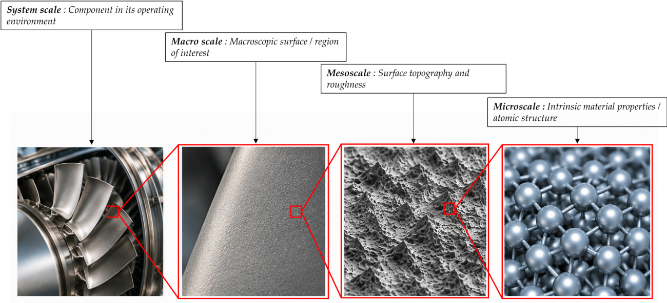
Figure 2.
Incident, reflected, and transmitted electromagnetic waves at a planar interface between two media. The electric and magnetic fields are denoted by and , respectively, and is the wavelength of the incident wave. The angles , , and denote the angles of incidence, reflection, and transmission,respectively, measured with respect to the interface normal, with .
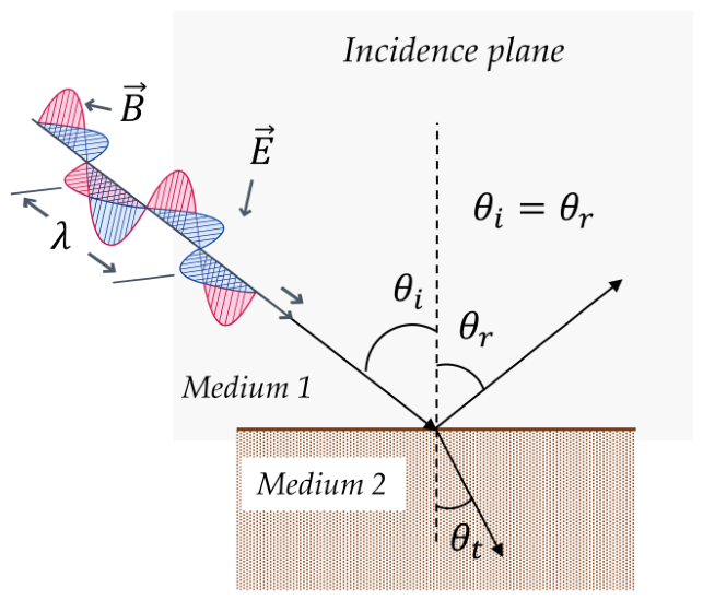
Figure 3.
Rectangular-groove geometry.
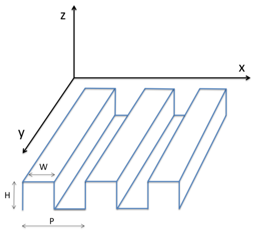
Figure 4.
Convergence study of the two solvers: (a) number of incident rays; (b) maximum number of reflections; (c) energy termination threshold; (d) number of Fourier harmonics retained in the RCWA.
Figure 4.
Convergence study of the two solvers: (a) number of incident rays; (b) maximum number of reflections; (c) energy termination threshold; (d) number of Fourier harmonics retained in the RCWA.
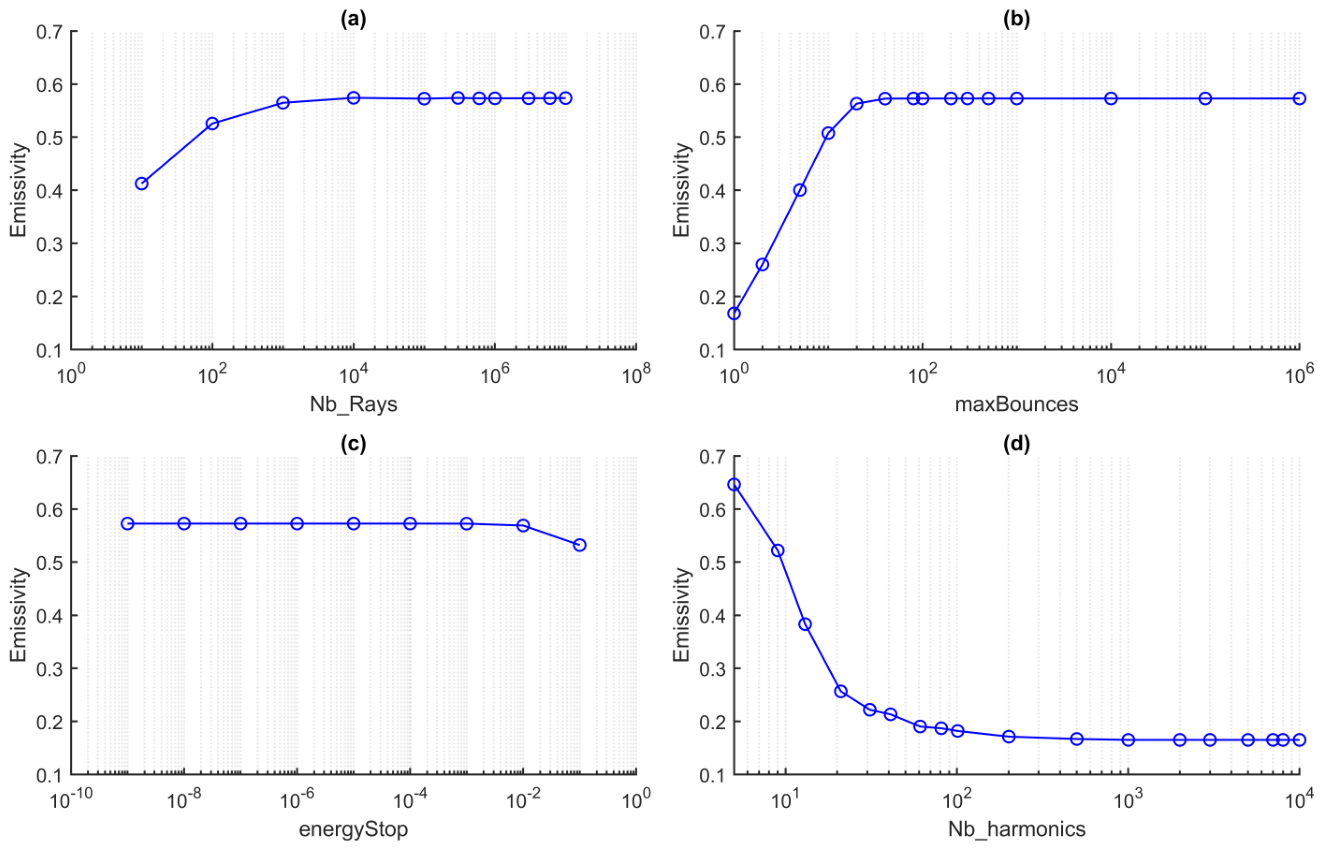
Figure 5.
Emissivity computed in this work and with the Ansys FDTD solver as a function of wavelength, for (a) TE polarization, (b) TM polarization and (c) unpolarized illumination.
Figure 5.
Emissivity computed in this work and with the Ansys FDTD solver as a function of wavelength, for (a) TE polarization, (b) TM polarization and (c) unpolarized illumination.
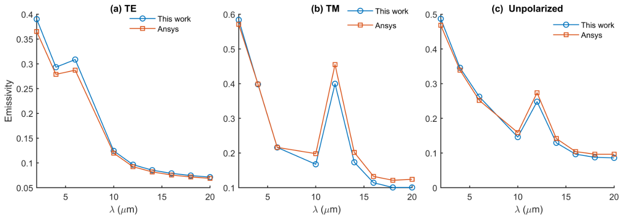
Figure 6.
Marginal mean emissivity predicted by the three models as a function of the period P, ridge width W, groove depth H, wavelength , and incidence angle .
Figure 6.
Marginal mean emissivity predicted by the three models as a function of the period P, ridge width W, groove depth H, wavelength , and incidence angle .
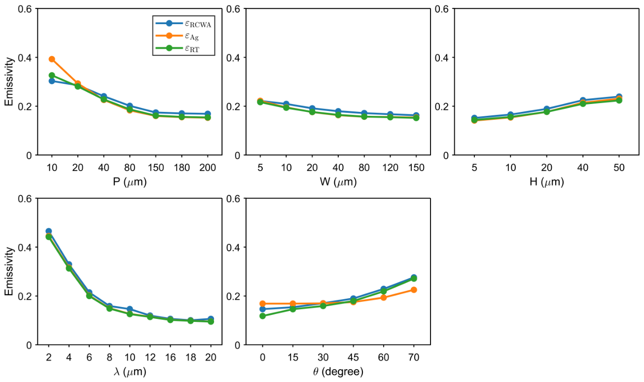
Figure 7.
Average number of rebounds for ray tracing as a function of the period P and groove depth H.
Figure 7.
Average number of rebounds for ray tracing as a function of the period P and groove depth H.
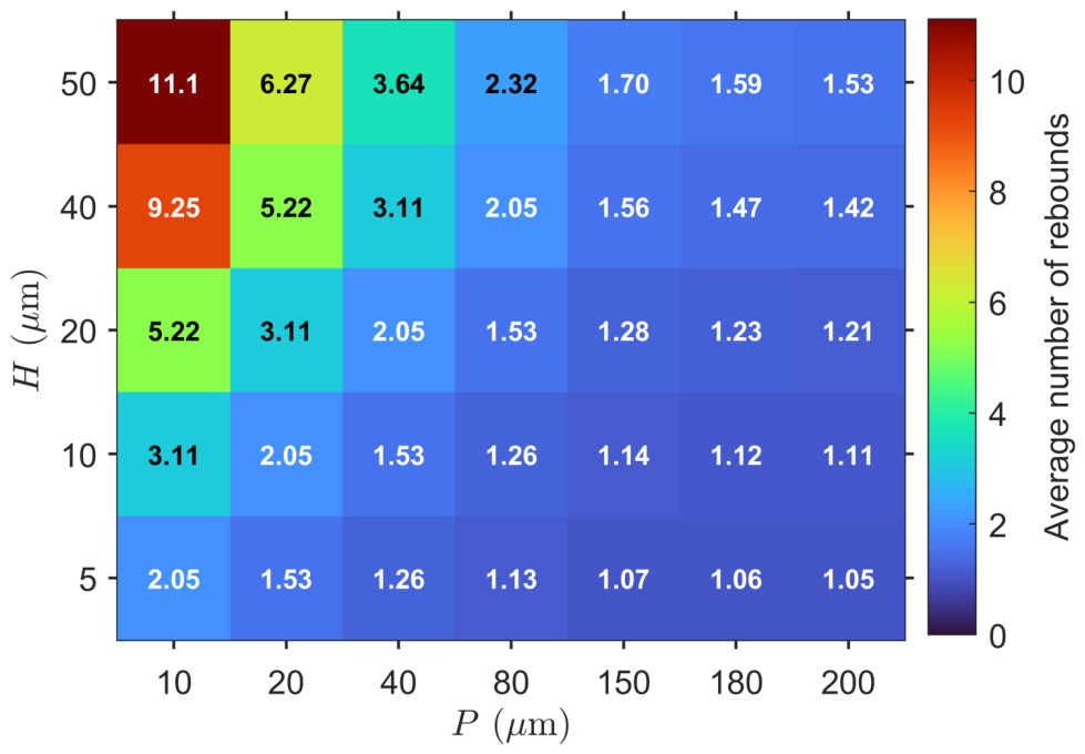
Figure 8.
Marginal mean relative error of the Agababov model and ray tracing with respect to RCWA as a function of the period P, ridge width W, groove depth H, wavelength , and incidence angle .
Figure 8.
Marginal mean relative error of the Agababov model and ray tracing with respect to RCWA as a function of the period P, ridge width W, groove depth H, wavelength , and incidence angle .
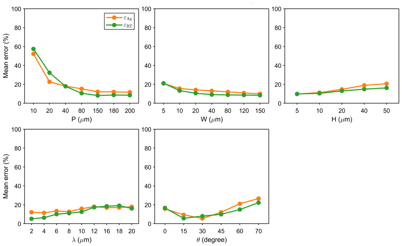
Figure 9.
Mean relative error of the Agababov’s model in the plane for the six investigated incidence angles. Cells marked with a cross correspond to configurations not represented in the numerical design.
Figure 9.
Mean relative error of the Agababov’s model in the plane for the six investigated incidence angles. Cells marked with a cross correspond to configurations not represented in the numerical design.
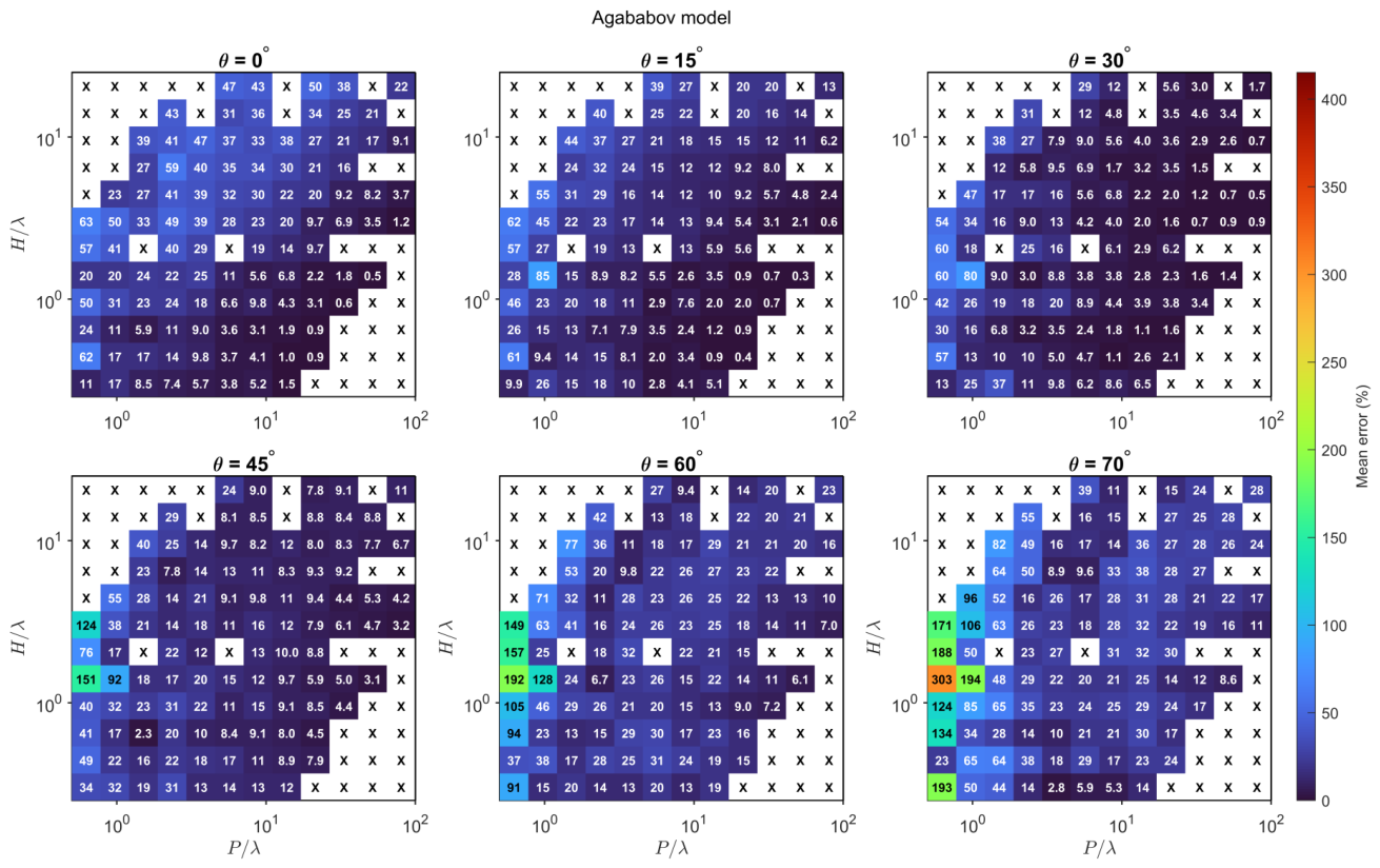
Figure 10.
Mean relative error of ray tracing in the plane for the six investigated incidence angles. Cells marked with a cross correspond to configurations not represented in the numerical design.
Figure 10.
Mean relative error of ray tracing in the plane for the six investigated incidence angles. Cells marked with a cross correspond to configurations not represented in the numerical design.
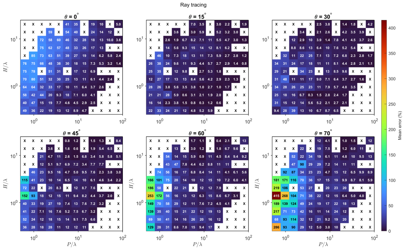
Figure 11.
Geometric-optics validity map reported by Tang et al. [7].
Figure 11.
Geometric-optics validity map reported by Tang et al. [7].
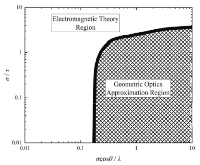
Figure 12.
Mean relative error of the Agababov model (left) and ray tracing (right) represented in the plane. The black boundary and hatched area correspond to the geometric-optics domain reported by [7].
Figure 12.
Mean relative error of the Agababov model (left) and ray tracing (right) represented in the plane. The black boundary and hatched area correspond to the geometric-optics domain reported by [7].
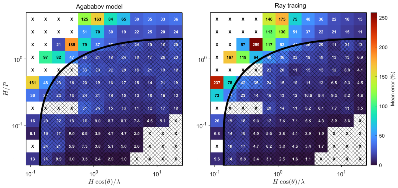

Table 1.
Main numerical parameters used in the ray-tracing simulations.
| Parameter | Value |
|---|---|
| Number of incident rays | |
| Maximum number of reflections | |
| Minimum remaining ray energy |
Table 2.
Parameter values explored in the simulated dataset.
| Parameter | Values |
|---|---|
| Period: P (µm) | 10, 20, 40, 80, 150, 180, 200 |
| Ridge width: W (µm) | 5, 10, 20, 40, 80, 120, 150 |
| Groove depth: H (µm) | 5, 10, 20, 40, 50 |
| Wavelength: (µm) | 2, 4, 6, 8, 10, 12, 16, 18, 20 |
| Incidence angle: (°) | 0, 15, 30, 45, 60, 70 |
Disclaimer/Publisher’s Note: The statements, opinions and data contained in all publications are solely those of the individual author(s) and contributor(s) and not of MDPI and/or the editor(s). MDPI and/or the editor(s) disclaim responsibility for any injury to people or property resulting from any ideas, methods, instructions or products referred to in the content. |
© 2026 by the authors. Licensee MDPI, Basel, Switzerland. This article is an open access article distributed under the terms and conditions of the Creative Commons Attribution (CC BY) license (http://creativecommons.org/licenses/by/4.0/).
Copyright: This open access article is published under a Creative Commons CC BY 4.0 license, which permit the free download, distribution, and reuse, provided that the author and preprint are cited in any reuse.