

Submitted:
09 October 2026
Posted:
12 October 2026
You are already at the latest version
Abstract
We develop an exact computational framework for studying preopen sets, preclosure, and candidate p-bounded witnesses in finite digital windows. The framework combines finite-topology operations, exhaustive subset enumeration, witness filtering, and comparisons between digital topologies. We prove the correctness of the principal algorithms, describe their computational complexity, and give a worked example. We also explain the distinction between a witness found in a finite window and a counterexample in an infinite digital space. Since the term p-bounded witness can depend on the particular problem under investigation, the witness predicate is treated as an explicit input to the algorithm rather than being assigned an unjustified universal meaning.
Keywords:
digital topology
; preopen sets
; preclosed sets
; preclosure
; finite digital images
; exhaustive search
; counterexamples
; p-bounded witnesses
1. Introduction
Finite digital windows provide a natural setting in which to test conjectures in digital topology. Their finiteness makes it possible to enumerate all subsets, compute their topological properties, and search systematically for configurations that satisfy specified hypotheses but violate a proposed conclusion.
The purpose of this section is to develop algorithms for three tasks:
- (i)
- computing all preopen subsets of a finite digital space;
- (ii)
- computing the preclosure of any given subset;
- (iii)
- searching for candidate p-bounded witnesses to a specified property or proposed counterexample.
These computations can support the comparison of different digital topologies and the discovery of explicit finite counterexamples. The general framework of digital topology is discussed in [1,2].
The basic topological computations are independent of the particular digital adjacency convention. Once a finite topology has been constructed, the algorithms apply to it directly. The interpretation of the final witness, however, depends on the exact mathematical definition of p-boundedness used in the problem.
2. Finite Digital Windows
Definition 2.1
(Finite digital window). A finite digital window is a finite set X equipped with a specified topology τ. In a lattice model, one may take
for positive integers m and d, together with a specified adjacency relation and a rule for constructing the topology.
Remark 2.2.
An adjacency relation alone does not uniquely determine a topology unless a construction rule is specified. In particular, the topology obtained by treating a window as a standalone digital space can differ from the subspace topology inherited from a larger digital space. Every computational experiment must state which convention is being used.
For a finite topological space , the interior and closure of are
and
The family of open sets can be stored explicitly. Alternatively, when the topology has a suitable finite-neighborhood representation, interior and closure can be computed from the neighborhood data.
Definition 2.3
(Preopen set). A subset is called preopen if
The family of all preopen subsets of X is denoted by .
Definition 2.4
(Preclosed set). A subset is preclosed if is preopen. Equivalently,
The family of all preclosed sets is denoted by .
Definition 2.5
(Preclosure). The preclosure of is
3. A Formula for Computing Preclosure
Theorem 3.1
(Preclosure formula). For every topological space and every ,
Proof.
Set
Since , monotonicity of interior and closure gives
We show that
Let U be any open subset of B. The set
is open because U is open and is closed. Moreover, it is contained in A, since
Consequently,
But this set is disjoint from . Therefore it is empty, and hence
Taking the union over all open subsets U of B yields
It follows that
Thus B is preclosed and contains A.
Now let F be any preclosed set with . Then
so
Since , we obtain
Therefore B is contained in every preclosed superset of A, and B is itself such a superset. It follows that
□
Remark 3.2.
Preclosure should not be confused with ordinary closure. In general,
The theorem provides a direct method for computing preclosure without enumerating all preclosed supersets.
4. Algorithm for Computing Preopen Sets
4.1. Exhaustive Algorithm
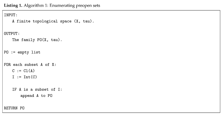
Let . There are exactly subsets of X, so exhaustive enumeration is finite.
Proposition 4.1
(Correctness of Algorithm 1). Algorithm 1 returns exactly the family .
Proof.
Every subset is examined. The algorithm records A if and only if
This condition is precisely the definition of preopenness. Therefore every preopen set is recorded, and no non-preopen set is recorded. □
4.2. Implementation Using Bit Masks
When , represent each subset by an n-bit integer. The i-th bit is 1 exactly when belongs to the subset. Inclusion, union, intersection, and complement can then be computed by bitwise operations.
For small and moderate n, it is useful to precompute
for every subset . This avoids repeated computations when the same subsets are used in multiple tests.
If the topology is given as a list of open sets, the interior can be computed by
Closure then follows from
5. Algorithm for Computing Preclosure
Proposition 5.1
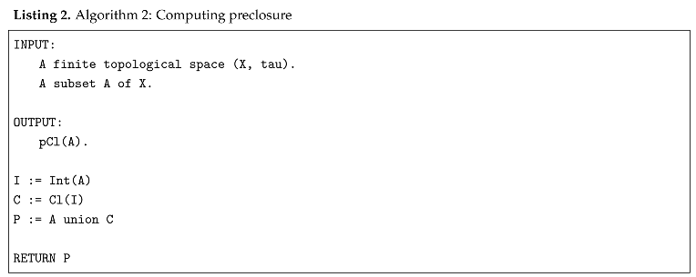
(Correctness of Algorithm 2). Algorithm 2 computes the preclosure of every subset .
Proof.
The algorithm returns
By the preclosure formula proved in the preceding section, this set is exactly . □
5.1. Independent Verification
For small finite spaces, one can verify the formula by a second, independent method:
- 1.
- enumerate all subsets F of X;
- 2.
- retain those satisfying ;
- 3.
- among those containing A, intersect all retained sets;
- 4.
- compare the result with .
Agreement between the two methods is a useful correctness test for a software implementation.
6. Developing Algorithms for Candidate p-Bounded Witnesses
6.1. Formalizing the Witness Condition
The term “p-bounded witness” must be defined in the context of the particular theorem under investigation. It may refer to a subset, a family of subsets, a sequence, or a configuration satisfying additional conditions.
Accordingly, we separate the general search procedure from the problem-specific predicate.
Definition 6.1
(Witness predicate). Let be a finite topological space and let denote auxiliary data required by a problem. A witness predicate is a specified Boolean-valued function
Its meaning must be determined by the precise definition of p-boundedness and the proposed assertion being tested.
Definition 6.2
(Candidate p-bounded witness). A subset is a candidate p-bounded witness if it satisfies a specified structural filter
and the witness predicate
Thus a candidate is retained exactly when
is true.
The structural filter may require, for example,
or that A be preopen, preclosed, or satisfy a relation involving . Such restrictions must come from the mathematical problem rather than being imposed without justification.
6.2. Generic Witness-Search Algorithm
Proposition 6.3
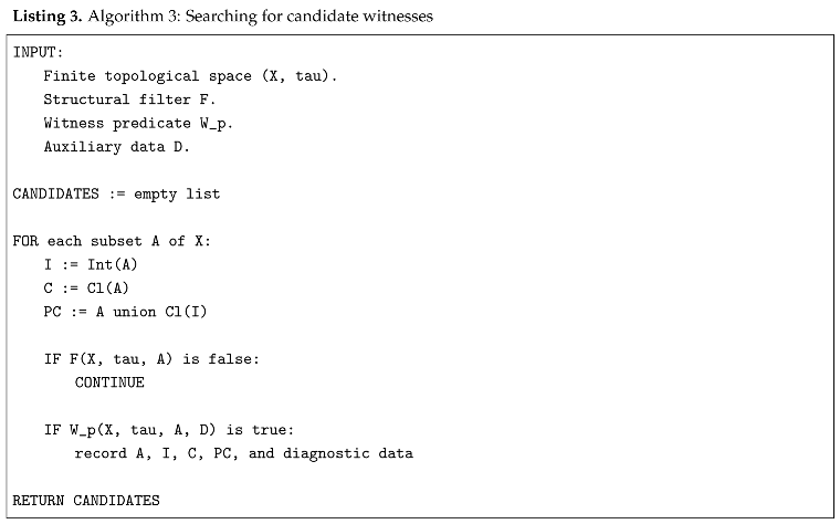
(Soundness relative to the specification). Every set returned by Algorithm 3 satisfies the structural filter and the witness predicate supplied as input.
Proof.
A set is recorded only after the algorithm has verified both
and
Hence every returned set satisfies both conditions. This establishes soundness relative to the supplied specification. The mathematical correctness of the implementation of must be verified separately. □
6.3. Searching for Counterexamples
Suppose a proposed assertion has the logical form
where H denotes the hypotheses and K the conclusion. A counterexample must satisfy
Thus, the correct search predicate is
possibly together with other conditions imposed by the definition of the problem.
Remark 6.4.
For a claim involving sequences, covers, or families of sets, a witness may not be representable by a single subset A. The search space must then consist of the appropriate finite tuples, families, or encoded sequences. The same filtering principle applies.
7. Illustrative Finite Example
Consider the topological space
We calculate the preopen sets and the preclosure of a particular subset.
Let
The only open set contained in A is ⌀. Therefore,
It follows that
To compute ordinary closure, recall that a point belongs to if every open neighborhood of that point meets A. The point a has the neighborhood disjoint from A. The only open neighborhood of c is X, which meets A. Consequently,
No nonempty open set is contained in , so
Therefore,
This example demonstrates that ordinary closure and preclosure need not agree:
For this three-point space, the algorithms can enumerate all eight subsets and classify each one exactly.
8. Comparing Different Digital Topologies
Let and be two topologies on the same finite set X. Compute
and compare the resulting families.
Useful comparison quantities include
and the symmetric difference
The latter identifies subsets that are preopen in one topology but not the other.
For every , one may also compare
This identifies subsets whose preclosures depend on the chosen topology.
A computational comparison should record:
- 1.
- the point set and the adjacency convention;
- 2.
- the construction of each topology;
- 3.
- the number of preopen sets;
- 4.
- the subsets whose preopen status changes;
- 5.
- the subsets whose preclosures differ;
- 6.
- the candidate witnesses found under each topology.
If the two digital spaces have different underlying sets, a comparison requires an explicitly specified identification or map between their point sets.
9. Complexity Analysis
Write and let be the cost of computing the interior or closure of a subset.
The exhaustive preopen-set algorithm has time complexity
up to the cost of testing set inclusion. The preclosure algorithm for one subset requires two topological operations and a union, so its complexity is
under a standard explicit-set representation.
If the witness predicate has cost , a direct exhaustive search has complexity
The exact bound depends on how the topology and witness data are represented.
Several optimizations are possible:
- 1.
- Bit masks: accelerate subset operations.
- 2.
- Caching: store interiors, closures, and preclosures for repeated use.
- 3.
- Symmetry reduction: search one representative from each orbit under a verified group of topology-preserving automorphisms, provided the witness predicate is invariant under that group.
- 4.
- Early filtering: apply inexpensive necessary conditions before evaluating an expensive witness predicate.
- 5.
- Counterexample minimization: attempt to remove points or reduce the window while preserving the witness condition.
A pruning rule is valid only when its necessary-condition or monotonicity argument has been established. In particular, preopenness should not be assumed to be monotone under arbitrary inclusion.
10. From Finite Windows to Infinite Digital Spaces
Suppose an infinite digital space is approximated by finite windows
A subset that is preopen in one finite window need not remain preopen in another. Both interior and closure depend on the topology in which they are computed.
Three logically different conclusions must be distinguished:
- 1.
- a counterexample exists in a particular finite window;
- 2.
- a witness persists under specified inclusions of windows;
- 3.
- the corresponding assertion fails in the infinite digital space.
The first conclusion follows from exhaustive search on the specified finite space. The second requires a persistence argument, and the third requires an infinite-space proof or a theorem connecting the finite models to the ambient space.
In particular, computations using standalone window topologies cannot automatically be interpreted as computations in the subspace topology inherited from an infinite digital space.
Proposition 10.1
(Scope of a finite exhaustive search). Let be a specified finite topological space, and suppose an algorithm examines every subset of X and correctly evaluates the relevant witness predicate. If the algorithm returns no witness, then no witness satisfying that predicate exists in .
Proof.
Every subset of X is examined. If a witness existed, the correct predicate evaluation would retain it. Since no witness is returned, none exists in the enumerated search space. □
This conclusion is restricted to the specified finite space and predicate. It does not imply that a witness is absent from every larger window or from the infinite space.
11. Validation and Reproducibility
A computational study should provide enough information for another researcher to reproduce its results.
For each experiment, record:
- 1.
- the finite point set;
- 2.
- the adjacency and topology conventions;
- 3.
- the representation of open sets or minimal neighborhoods;
- 4.
- the definitions used for preopen and preclosed sets;
- 5.
- the implementation of interior, closure, and preclosure;
- 6.
- the exact witness predicate and all auxiliary data;
- 7.
- any symmetry reductions or pruning rules;
- 8.
- the complete encoding of each reported witness;
- 9.
- an independent verification of each claimed counterexample.
For small windows, useful consistency checks include
and
One should also verify the topology axioms for any topology generated by a digital adjacency rule.
A picture of a digital configuration can be helpful, but it should be accompanied by the precise point set, topology, witness predicate, and diagnostic computations.
12. Conclusion
The algorithms developed here provide a systematic framework for computing preopen sets, preclosure, and candidate p-bounded witnesses in finite digital windows.
The main computational advantages are:
- 1.
- exhaustive and exact classification of preopen subsets;
- 2.
- direct computation of preclosure using ;
- 3.
- systematic searches for counterexamples under an explicit witness predicate;
- 4.
- reproducible comparisons between different digital topologies;
- 5.
- diagnostic data for investigating whether finite witnesses persist under enlargement of the window.
The essential methodological principle is to separate exact finite-topology calculations from the problem-specific definition of a p-bounded witness. With that separation, computational experiments can provide reliable evidence, expose candidate counterexamples, and guide the development of proofs without mistaking finite verification for a theorem about an infinite digital space.
References
- Khalimsky, E.; Kopperman, R.; Meyer, P. R. Computer graphics and connected topologies on finite ordered sets. Topol. Its Appl. 1990, 36, 1–17. [Google Scholar] [CrossRef]
- Kong, T. Y.; Roscoe, A. W.; Rosenfeld, A. Concepts of digital topology. Topol. Its Appl. 1992, 46, 219–262. [Google Scholar] [CrossRef]
- Mashhour, A. S.; Abd El-Monsef, M. E.; El-Deeb, S. N. On precontinuous and weak precontinuous mappings. Proc. Math. Phys. Soc. Egypt 1982, 53, 47–53. [Google Scholar]
- Kuratowski, K. Topology, Vol. I; Academic Press: New York, 1966. [Google Scholar]
Disclaimer/Publisher’s Note: The statements, opinions and data contained in all publications are solely those of the individual author(s) and contributor(s) and not of MDPI and/or the editor(s). MDPI and/or the editor(s) disclaim responsibility for any injury to people or property resulting from any ideas, methods, instructions or products referred to in the content. |
© 2026 by the authors. Licensee MDPI, Basel, Switzerland. This article is an open access article distributed under the terms and conditions of the Creative Commons Attribution (CC BY) license (http://creativecommons.org/licenses/by/4.0/).
Copyright: This open access article is published under a Creative Commons CC BY 4.0 license, which permit the free download, distribution, and reuse, provided that the author and preprint are cited in any reuse.