

Submitted:
10 October 2026
Posted:
10 October 2026
You are already at the latest version
Abstract
Constrained-layer damping in sandwich floors and wall panels is usually analysed with uniform faces and a uniform core, while phononic treatments of periodicity address stop bands rather than the first few forced resonances of a finite plate. A seven-degree-of-freedom rectangular finite element is formulated here for a three-layer sandwich plate whose face thicknesses and core shear moduli vary in the plane as separable cosines. The kinematics follow Mead–Markus: Kirchhoff faces, first-order shear in a soft Kelvin–Voigt core, and a single transverse deflection. Membrane interpolation is bilinear; bending uses the Adini–Clough–Melosh incomplete quartic. A Navier–Galerkin sine series on two single-mass plates verifies the element to within one frequency step. On the modulated plate the Galerkin first peak is f1 = 8.93 Hz and the finite-element first peak is f1 = 9.57 Hz; on the uniform plate both methods give f1 = 7.66 Hz. These three frequencies belong to the materials and planform of those two plates. Three archives then isolate core periodicity, face periodicity, and the layout of a fixed total attached mass. The first resonance of the core-campaign reference stays near 12 Hz; its height follows the area-averaged storage modulus. The two mean face thicknesses c1m and c3m dominate the higher peaks; at fixed sum an unequal split is stiffer than two equal faces. Relocating the attached masses onto midlines or a diagonal rearranges the centre-point frequency-response function more than reweighting the 3 × 3 lattice. The spectra contain no phononic stop band.
Keywords:
sandwich plate
; constrained-layer damping
; viscoelastic core
; periodic modulation
; finite element
; Galerkin verification
; harmonic response
1. Introduction
Sandwich plates with a thin viscoelastic core are a standard means of reducing flexural vibration. The faces constrain the core, so bending drives the core into shear and dissipates energy. That mechanism is known as constrained-layer damping (CLD). In buildings a sandwich of this kind is used as a lightweight floor or a wall panel of one bay. The faces are a stiff isotropic polymer composite and the core is a soft viscoelastic polymer. These are modelling values for a structural sandwich, not a named commercial product and not a sub-millimetre damping tape. The viscoelastic core attenuates flexural vibration of that floor or partition under base motion. Kerwin [1] and DiTaranto [2] identified it for beams. Mead and Markus [3] then gave the three-layer kinematics that still underlie most forced-vibration analyses of the stack. Yan and Dowell [4] extended the governing equations to sandwich plates and beams. Rao [5] gave the frequencies and loss factors of sandwich beams for the principal boundary conditions. Finite-element implementations follow the same template, with the core represented either by a complex modulus [6,7,8,9] or by a frequency-domain viscous or fractional operator [10,11,12,13]. Layerwise and zig-zag theories refine the through-thickness kinematics when the core is thick or compressible [14,15,16,17,19,20,21]. Recent plate-level studies still treat a uniform or piecewise-uniform stack: spectral collocation of a viscoelastic sandwich [22], embedded viscoelastic plies [23], soft-core delamination [24], auxetic cores [25], functionally graded constraining layers [26], and active or hybrid CLD and layout optimisation [27,28,29,30,31]. Reviews of viscoelastic damping and of hybrid active–passive treatments set the broader design context [32,33,34].
Those CLD models treat each layer as uniform, or at most piecewise uniform, in the plane. A second literature treats periodicity as a wave-control device. Phononic crystals, locally resonant plates, and ribbed or patched waveguides are analysed through dispersion diagrams and attenuation bands [35,36,37,38,39,40,41,42]. Honeycomb, truss and other discrete cores introduce periodicity through a microstructure [43,44,45], not through a prescribed continuum field on an otherwise homogeneous sandwich. Viscoelastic cores that are periodic by cells do produce stop bands on sandwich beams and plates [46,47,48,49]. Cupiał and Nizioł [50] analysed a viscoelastic mid-layer that remains uniform. The two streams therefore leave an intermediate case: a sandwich plate whose face thicknesses and core shear moduli vary slowly across the planform. That case has already been reduced by a Navier–Galerkin projection of the coupled face-membrane and core-shear equations, first on a sandwich beam with harmonic parameters [51] and then on simply supported sandwich plates with cosine-modulated faces, a viscoelastic core and distributed supported masses [52,53,54]. Those reductions supply frequency-response operators, but they remain tied to a Navier basis on a single rectangle.
That slow modulation is not a phononic crystal. Its wavelength is comparable to the plate, so a coarse structural mesh cannot resolve a Bragg or local-resonance gap, and none should be claimed. It is nonetheless strong enough to change the area-averaged stiffness, the local shear lever arm between the faces, and therefore the forced frequency-response function (FRF). Such fields arise in tapered faces, in a core whose thickness or storage modulus is patterned on the scale of the plate, and as the leading long-wave residual of an imperfect lay-up. A designer who must place or suppress the first few resonances under base motion then needs that FRF: which peaks move, and by how much. A Bloch band diagram does not answer that question.
The present paper addresses the intermediate case with a rectangular finite element that can be assembled on an arbitrary mesh and mass layout. The element is reproduced from the stated kinematics and interpolation: Kirchhoff faces, first-order shear in a Kelvin–Voigt core, bilinear membrane fields, Adini–Clough–Melosh bending [8,55], and cosine modulation of both faces and core. The harmonic problem is solved under base acceleration and attached point masses. Before any parametric scan, a Navier–Galerkin sine series of the same family [52,53] verifies the element on two single-mass plates that share the planform and the total attached mass of the later campaigns: one plate is cosine-modulated and one is uniform. Three archives then isolate independent controls. The first varies the core wavenumbers and the core thickness. The second varies the four face wavenumbers, the relative thickness amplitude, and the two mean face thicknesses. The third relocates a fixed total attached mass on the same plate. The first three centre-point FRF peaks are reported as grid values. That separation is the novelty of the study, and it is numerical. Uniform CLD elements do not carry an in-plane cosine field, and phononic analyses do not give the first forced peaks of a finite modulated plate. The Galerkin reductions do both, but only on one simply supported rectangle. The element is not tied to that basis: the same matrices accept any rectangular mesh and any set of nodal masses. No experiment is used to support these comparisons.
The numerical scope is a soft core with Young’s modulus neglected (), omitted rotatory inertia, a Kelvin–Voigt law whose loss factor grows linearly with frequency [6,12,56], and a rectangular mesh on which the reported spectra have converged. The cosine fields are not claimed to produce phononic stop bands, and no experiment is reported.
2. Kinematics and Finite-Element Formulation
2.1. Kinematics and Constitutive Model
The plate occupies the rectangle . Figure 1 shows the simply supported planform with nine equal point masses on a lattice. Figure 2 is the through-thickness stack: a top face of thickness , a core of constant thickness , and a bottom face of thickness . The core mid-plane is , so the core occupies . The face mid-planes are
The bottom-face/core interface is and the top-face/core interface is . Subscripts c, v and p denote the top (constrained) face, the viscoelastic core and the bottom face.
Face thicknesses and the core shear moduli vary periodically. In global coordinates ,
The four face wavenumbers are independent: act only on , and act only on . If a wavenumber vanishes, the corresponding cosine is identically 1, so that face varies in at most one direction; if both wavenumbers of a face vanish, that face has the uniform thickness . The storage and loss coefficients of the core share the pair . Thus and have the dimension of stress, while and have the dimension of stress times time. If every amplitude vanishes, the plate is uniform. Element integrals use a local frame centred on the element, with and .
Figure 3 shows f for two isotropic pairs. The area average of f on is , where and for . Integer wavenumbers therefore leave the mean modulus or mean thickness unchanged, while gives . The cubic mean that enters bending stiffness still depends on the amplitude when , because .
The kinematic and constitutive hypotheses are as follows. Deformations are small and the strain–displacement relations are linear. The three layers are perfectly bonded and share a z-independent deflection w. Each face is an isotropic Kirchhoff plate in plane stress; face shear is neglected. The core in-plane displacement is linear in z (first-order shear). The core shear law is Kelvin–Voigt,
with and . is the Young’s modulus of layer , that is the in-plane direct stiffness, and is Poisson’s ratio. is that modulus for the core. It is not a shear modulus: core shear is carried by and . The formulation retains core membrane and bending stiffness when . In the examples that stiffness is neglected: changes the reported spectra only negligibly, and it is set to zero. Kinetic energy retains mid-plane translation of each layer and omits rotatory inertia. Variable thickness is treated locally: interface continuity and use the thickness at the integration point.
The independent mid-plane fields are , and w. The Kirchhoff rotations are
so and are not additional independent fields. A nodal generalised displacement is
Through the thickness of each face,
Interface continuity at then gives
and the analogous pair for v. Linear interpolation through the core, together with , yields the Mead–Markus core fields
The shear strain is produced by the relative in-plane slip of the faces together with the lever arm , which is the distance between the face mid-planes. In terms of (8), and .
Membrane strains and the common Kirchhoff curvature are the engineering measures [4,50]
with and from (12)–(13). The curvature is the engineering curvature, linear in the second derivatives of w. That linearisation is the small-displacement hypothesis stated above: the nonlinear terms of the Green strain are omitted. Each isotropic layer uses the plane-stress matrix
membrane stiffness and bending stiffness . The leading diagonal entries are direct stiffnesses. The last diagonal entry is the in-plane shear stiffness . is not the transverse shear stiffness of the core. The local strain in layer is with .
2.2. Finite-Element Discretisation
A uniform partition of into rectangles of size and is the default mesh. If an attached mass does not lie on a node, an additional grid line is inserted through that station, so some rectangles are smaller than the nominal cell; the element below is written for a general rectangle. Each element has four nodes, ordered anticlockwise from the lower-left corner, and 28 degrees of freedom .
The four membrane fields , , and are interpolated with the complete bilinear monomials . The deflection uses the ACM incomplete quartic [8,55]
The seven interpolated fields are collected in a monomial matrix , whose last two rows are and acting on the coefficients of (18). Collocating at the four nodes produces the configuration matrix . The shape-function matrix is , with rows so that , , , , , and . The core interpolants follow from (12)–(15) and (8):
hence , , and .
ACM interpolation enforces and inside the element, but the normal rotation is not continuous across element edges. The element is therefore a nonconforming thin-plate rectangle. Membrane fields are .
The strain–displacement matrices are
When and vary, and depend on thickness, so contains and terms. The shear rows and use the local thicknesses but not their derivatives. That is the local-thickness approximation stated with those hypotheses.
On the local domain , with a and b equal to half the element sides, the element matrices are
If , the core membrane and bending blocks vanish and is not formed. The only damping in is core shear viscosity. A base acceleration produces the consistent inertial load
The integrals are evaluated by four-point Gauss–Legendre quadrature in each local direction, with , , and sampled at the Gauss points. The element matrices, the assembly and the harmonic solve are an in-house implementation in MATLAB. No commercial finite-element package is used. The global matrices , , and are assembled by the standard element-to-global map [8,9].
All four edges are simply supported. On and the essential conditions are ; on and they are . The in-plane displacement normal to the edge and the rotation associated with the normal slope remain free (moment-free natural condition). Constrained degrees of freedom j are treated by zeroing the corresponding rows and columns, setting and , where is the largest unconstrained ratio of diagonal stiffness to diagonal mass; the associated damping diagonal is left at zero.
Each attached mass at a mesh node is added to the five translational entries of that node’s block (rotations receive no mass), and is added only to the transverse force for . Those five entries are , , , and w, and each receives the full . The in-plane inertia is therefore assigned to both faces. That choice is intentional: each face receives the full , rather than a share of one mass or a fixture bonded to one face only. The transverse entry receives once, and that is the inertia which shifts the base-driven flexural spectrum. If the two faces have the same in-plane velocity , the two in-plane entries together store kinetic energy , twice the energy of a single rigid mass moving with one face. The tabulated spectra use this five-entry assembly and have not been recomputed with a one-face attachment. If does not coincide with an existing node, an additional grid line is inserted so that every mass sits on a node.
2.3. Harmonic Analysis
After assembly the discrete system is
The steady state satisfies
The sparse complex system is factored at each frequency. The operator is identical to a complex-stiffness assembly that uses [6,11]. The corresponding loss factor therefore grows linearly with frequency. The reported centre-point spectrum is
plotted as against .
The same operator (29) is used to verify the element against an independent Navier–Galerkin reduction [51,52,53] on two simply supported rectangles with identical faces and one central mass: a cosine-modulated plate and the corresponding uniform plate. The deflection is
with . The membrane fields use the compatible Navier pairs (cosine–sine for u and sine–cosine for v) and are condensed by the in-plane weak form, so the reduced unknown is the coefficient vector . The reduced mass, damping and stiffness come from the same face-membrane, face-bending and core-shear energies as (24)–(26), restricted to and to a common face-wavenumber pair; they are not fitted to the FEM spectrum. The centre-point amplitude reconstructed from (31) is compared with (30) on the same frequency grid.
3. Results and Discussion
Table 1 lists the locked data of the primary geometry. The frequency samples are (188 frequencies). The frequency step is ; every quoted peak is a grid point, not an interpolated maximum. Nine equal point masses occupy a lattice. The nine stations and the common mass are listed in Table 5. The plate is partitioned into a mesh of rectangular elements, and every attached mass lies on a node. The spectra on this mesh have converged.
Two campaigns lock complementary groups so that core periodicity is not confounded with face periodicity. The core campaign varies and holds the faces at , , , , and . The face campaign varies the face fields and holds the core at and ; wavenumber cases are labelled K and amplitude or thickness cases are labelled F. Twenty wavenumber plates (K01–K20) isolate five geometric contrasts, with and locked: equal wavenumbers ; aligned one-dimensional stripes; orthogonal top and bottom stripes; top–bottom mismatch, including one-sided periodicity; and rectangular cells with . Mean-thickness cases hold and , and include both and . Face-campaign F01 and wavenumber K01 are the same plate and serve as the face-campaign reference. Core C01 is a different plate and is used only as the core-campaign reference. A third archive holds that same core-C01 plate and varies only the attached-mass layout at fixed ; the cases are labelled D. Stations and masses are listed in Table 6.
A peak in this section is a local maximum of on the frequency grid. The first three maxima are denoted , and , where .
Figure 4 verifies the finite-element FRF against the Galerkin series (31) on two single-mass plates with , , and . The periodic plate has and relative face amplitude ; the uniform plate sets every amplitude to zero. The two methods use the same geometry, the same frequency grid and the same operator (29); both plates are drawn on Figure 4, with FEM as solid lines and the Galerkin series as markers. These spectra are not overlaid on the campaign.
On the periodic plate the first peak differs by one grid step: Galerkin gives , FEM gives . The next two peaks coincide at and . The first-peak heights are (Galerkin) and (FEM), a gap of .
On the uniform plate both methods place the first two peaks at and , and differs by ( versus ). The third peak differs by one grid step: Galerkin , FEM . The element therefore reproduces the series frequencies to within one grid step on both a modulated and an unmodulated stack, and it is accepted for the parametric campaigns. The values , and are the first peaks of these two verification plates. They move if the materials or the planform change, and they are not properties of the element. The two locked campaign references are different plates and are never overlaid: face-campaign F01 has , whereas core C01 has . All later comparisons stay inside a single campaign.
3.1. Core Shear-Modulus Modulation and Thickness
Table 2 and Figure 5 collect Series I (isotropic ), Series II (thickness at ) and Series III (uniform core and one-dimensional stripes). Raising the core wavenumber from to 1 drops from to 0 and therefore drops the mean storage modulus from to . The first-peak height rises from to (C02), which is the largest first-peak change in Series I, and moves down by one grid step. Further integer or half-integer wavenumbers (C03, C04) stay within of that height. The spatial pattern of the core, once the mean modulus is fixed, is a weak perturbation of on this mesh.
Thickness acts on both mass () and shear strain (). From C05 to C08, falls from to and rises by one step. The third peak moves down in frequency and down in height, so a thicker core is not a pure mass addition.
The uniform high-modulus core C09 (, , ) gives the smallest first peak in Table 2, at . One-dimensional stripes (Figure 6) lie between C01 and C09 when is large (C10) and near the integer-wavenumber plates when (C11). That ordering supports a mean-modulus reading: periodicity of and changes mainly by changing and , not by opening a gap.
On the present mesh, core periodicity therefore acts as a mean-property perturbation. The factor ranks among C01, C02, C10, C11 and C09. Cases with the same differ by at most in , which is small beside the gap between C02 and C09. A design that only “adds periodicity” to without changing therefore moves the fundamental FRF little. This ranking is the continuum counterpart of a long-wave homogenisation argument: when the modulation wavelength is comparable to the plate, the first global mode samples an area average more than a unit-cell band structure [36,41].
Core thickness adds mass, reduces , and changes the lever arm in (14). decreases as increases from to , then changes by less than from C07 to C08. The return therefore diminishes once the core is several times the face thickness, which is consistent with classical CLD optimisation: an excessively thick soft core no longer increases the constrained shear in proportion to the added mass [1].
3.2. Face-Thickness Modulation
Table 3 and Table 4 and Figure 7, Figure 8 and Figure 9 summarise the face campaign. Here and are the top-face wavenumbers in X and Y, while and are the bottom-face pair; they are independent in (2)–(3).
K01–K04 keep the four equal and raise that common value from to 2 (Table 3, Series I; Figure 7a). Those cases leave at or . The second peak falls from (K01) to (K04), a shift of about , while stays near . Raising all four wavenumbers together therefore rearranges the second and third resonances more than it changes the fundamental amplitude.
The remaining sixteen plates let the four wavenumbers differ (Table 3, Series II–V; Figure 8). On these symmetric faces, exchanging the top pair with the bottom pair leaves unchanged to the reported precision: K09 coincides with K10, K13 with K14, and K15 with K16. Aligned x-stripes (K05) and y-stripes (K07) at half-integer wavenumber differ from each other by only in and share , about above the two-dimensional reference K01. The orthogonal arrangement K09 matches K05 in , and , and differs by in . Thus, at the centre point, the relative orientation of the two faces is a weaker control than whether the modulation is one- or two-dimensional, and the latter acts partly through : a one-dimensional half-integer stripe has , whereas K01 has .
Direction does appear once a wavenumber is an integer. Y-aligned integer stripes (K08, K20) place at , one grid step below the corresponding x-aligned plates (K06, K19). The planform is not square (, ), so the two directions are not equivalent; the centre-point FRF feels that anisotropy, but still only at the level of one frequency step.
One-sided periodicity (K15, K16) gives the largest first-peak change in Table 3: at . The inactive face has both wavenumbers zero, so its thickness is the uniform value rather than a zero-mean ripple about . That is again a mean-thickness shift, not a Bragg effect. Rectangular cells with put between the bounding equal-wavenumber cases: K17 and K18 () sit between K01 () and K02 (); K19 and K20 () sit between K01 and K04 ().
Relative amplitude at fixed and moves from () to (). The first-peak height stays inside . Because grows with even when is held fixed, the upward drift of and is the expected stiffening, not evidence of a Bragg mechanism.
Mean face thickness is the strongest control in the archive. Symmetric faces with and give at and at ; falls from to . The second peak more than doubles in frequency over that interval. Those shifts dwarf the core-wavenumber effect in Table 2.
The two means need not be equal (Table 4, last block; Figure 9b). Exchanging with leaves unchanged to the reported precision: F10 coincides with F11, and the same inversion holds for an untabulated pair at . The faces have identical moduli and densities, so turning the stack over does not change the centre-point spectrum. What matters is the unordered pair .
At fixed sum , the equal split F01 has , the mild split F12 has , and the split F10 has with one grid step higher. The same ordering appears at sum : F13 () lies above F08 () in , and . The lever arm in (14) depends on , hence only on the sum, but the bending stiffness of each face scales as . For a fixed sum the convexity of on gives , with equality only when , so an unequal pair is the stiffer plate. The difference that enters (12) does not break the inversion symmetry of on this mesh.
Face periodicity therefore enters mainly through and the higher resonances. To move the fundamental under base excitation, change the pair . To rearrange and at nearly fixed , change the common wavenumber, the thickness amplitude, or the split of a fixed sum. Assigning distinct is a finer correction on this mesh.
3.3. Attached-Mass Layout
The eight layouts in Table 6 keep the core-C01 plate and the total attached mass . Each row of that table gives the occupied stations and . D01 occupies all nine nodes of Table 5 with equal mass and is identical to core C01.

Table 5.
Locations of the nine equal point masses on the campaign plate (, ). Each mass is . The ordering matches the MATLAB driver (rows of increasing Y, then X).
Table 5.
Locations of the nine equal point masses on the campaign plate (, ). Each mass is . The ordering matches the MATLAB driver (rows of increasing Y, then X).
| k | X () | Y () | () |
|---|---|---|---|
| 1 | 234 | ||
| 2 | 234 | ||
| 3 | 234 | ||
| 4 | 234 | ||
| 5 | 234 | ||
| 6 | 234 | ||
| 7 | 234 | ||
| 8 | 234 | ||
| 9 | 234 |
Table 6.
Mass-layout peaks on the core-C01 plate at fixed . Stations lie on the lattice of Table 5 (coordinates in , masses in ). D01 is identical to core C01. Frequencies are grid values in ; .
Table 6.
Mass-layout peaks on the core-C01 plate at fixed . Stations lie on the lattice of Table 5 (coordinates in , masses in ). D01 is identical to core C01. Frequencies are grid values in ; .
| Case | Stations and | ||||||
|---|---|---|---|---|---|---|---|
| D01 | nine nodes of Table 5; | ||||||
| D02 | same; on | ||||||
| D03 | same; on | ||||||
| D04 | , , , , ; | ||||||
| D05 | , , , , ; | ||||||
| D06 | , , ; | ||||||
| D07 | , , ; | ||||||
| D08 | , , ; |
Reweighting the same nine stations is a weak perturbation (Figure 10a). A split along Y (D02) or along X (D03) leaves and moves by at most . The first centre-point peak therefore feels the total mass and the occupied lattice, not a mild row-to-row imbalance.
Relocating the mass onto fewer stations is stronger (Figure 10b). The five-point cross (D05) and the three-point midlines (D06, D08) put more mass on the antinode of the fundamental, so falls to or and rises. The five-point corner-and-centre set (D04) does the opposite: rises one grid step to , because four of the five masses sit nearer the simply supported edges. The three-point diagonal (D07) keeps but drops from to , the largest second-peak shift in Table 6. Thus, at fixed total mass, the useful control is which nodes carry the mass, not a rearrangement of weights on the full lattice. These shifts remain smaller than a change of both mean face thicknesses, and they must not be compared with Table 3 and Table 4: those tables use a different locked face pair.
None of the FRFs exhibits a stop band. The modulation spans half a wave to two waves across the plate, so its wavelength is comparable to the structural modes, and the mesh resolves only those long waves [36,41,47,48]. The spectra should not be read as a phononic-crystal calculation of the kind reported for piecewise-periodic viscoelastic cores [46,47,49].
The Kelvin–Voigt operator over-damps high frequency relative to a constant-loss or fractional model [11,12,56]. Peak heights above about 40 are therefore more model-dependent than . The spectra are computed on a mesh of rectangular elements, with every attached mass on a node. Those results have converged. This mesh is adequate for the first few global modes of a simply supported rectangle [8,9]; it cannot represent steep thickness gradients if the wavenumbers were raised much beyond 2. The frequency step is fixed: . A one-step change in a quoted peak is at that resolution. It is not a smaller shift that the sampling has resolved. Soft-core kinematics omit core compression, which matters for thick or soft cores [14,15,19,24]. On the face-thickness archive the fundamental lies between about and about . ISO 10137 and AISC Design Guide 11 judge floor vibration by frequency-weighted acceleration under walking, not by a strength limit [57,58]. Design Guide 11 treats a floor near or below about as one that can respond resonantly to a walking harmonic, and a stiffer floor as one whose response is essentially transient [58]. The curves in this paper are base-acceleration spectra of a simply supported plate. They are not that walking-load check. They do show where a bay-sized sandwich floor or partition of this construction sits relative to the division those documents use. A lightweight aluminum-foam sandwich slab has been compared with a conventional floor frame under dynamic loading [59]. Crowd walking-load models for vibration serviceability have been compared [60]. The tables describe this element, this grid and this constitutive law.
4. Conclusions
A Mead–Markus rectangular element is formulated for a sandwich plate whose face thicknesses and core shear moduli vary slowly across the planform, and the centre-point frequency-response function is computed under base acceleration and attached point masses. The main conclusions are as follows.
- A Navier–Galerkin sine series verifies the element on two single-mass plates that share the later planform and the later total attached mass, one cosine-modulated and one uniform. First-peak frequencies differ by one grid step on the modulated plate and coincide on the uniform plate; the next peaks agree to the same tolerance. The three later archives lock different layer pairs and are not interchangeable.
- Core periodicity acts mainly through the area-averaged storage modulus. A uniform high-modulus core gives the smallest first peak; an integer-wavenumber core, whose modulation averages to zero, gives the largest. Once that mean is fixed, the in-plane pattern of the core is a weak perturbation. Adding periodicity without changing the area average therefore moves the fundamental little.
- The two mean face thicknesses are the strongest control. Raising both means together moves the fundamental over a far wider interval than any core-wavenumber change in the archive, and it more than doubles the second-peak frequency. At a fixed sum an unequal split is stiffer than two equal faces; exchanging the two means leaves the centre-point spectrum unchanged. Distinct face wavenumbers and the relative thickness amplitude rearrange the higher peaks at a nearly fixed fundamental.
- At fixed total attached mass, occupying a midline, a cross or a diagonal rearranges the centre-point spectrum; reweighting the full lattice does not.
- None of the spectra contains a phononic stop band. The cosine fields span at most two waves across the plate, so the calculation is a long-wave forced-response study, not a dispersion analysis of a phononic crystal. The Kelvin–Voigt core over-damps high frequency relative to a constant-loss model, rotatory inertia is omitted, and the reported spectra have converged on the rectangular mesh used here. The tabulated peaks describe this element, this grid and this constitutive law. Differences of one frequency step remain at the resolution . A comparison with a laboratory frequency-response test, or with an existing solid or shell formulation, was not available for the modulated plates and is left as later work. Two routes are open. A base-excitation test on a simply supported rectangle of the same planform can be set against the first three centre-point peaks. Separately, the uniform plate can be rebuilt with shell faces and a solid core whose shear modulus is , and compared with the Galerkin series of this paper, before the cosine fields are put back.
Author Contributions
Conceptualization, Z.-G.R.; methodology, L.X., Z.-G.R. and H.L.; software, L.X. and Z.-G.R.; validation, L.X. and Z.-G.R.; formal analysis, L.X. and H.L.; investigation, L.X. and H.L.; resources, Z.-G.R.; data curation, L.X.; writing—original draft preparation, L.X.; writing—review and editing, Z.-G.R. and W.W.; visualization, L.X.; supervision, Z.-G.R.; project administration, Z.-G.R.; funding acquisition, L.X. and Z.-G.R. All authors have read and agreed to the published version of the manuscript.
Funding
This research was funded by the Full Time Researchers from Zhejiang University Hainan Research Institute Launch Project, grant number 0210-6602-2025042336, and the Talent Introduction Project of Hubei Polytechnic University, grant number 24xjz22R.
Institutional Review Board Statement
Not applicable.
Informed Consent Statement
Not applicable.
Data Availability Statement
The centre-point spectra for the core, face, wavenumber and mass-layout series are archived as plain-text frequency-response files together with the finite-element drivers. Further data are available from the corresponding author upon reasonable request.
Conflicts of Interest
The authors declare no conflicts of interest.
Nomenclature
| in-plane coordinates on | |
| local element coordinates | |
| z | through-thickness coordinate; core mid-plane at |
| top-face, bottom-face and core thicknesses | |
| mean thicknesses of the top and bottom faces | |
| thickness amplitudes of the top and bottom faces | |
| relative face-thickness amplitude | |
| top-face wavenumbers in X and Y | |
| bottom-face wavenumbers in X and Y | |
| core-modulus wavenumbers in X and Y | |
| Young’s modulus (direct stiffness) and Poisson’s ratio of layer | |
| core Young’s modulus; neglected in the examples () | |
| core storage modulus and Kelvin–Voigt viscosity | |
| mean and amplitude of | |
| mean and amplitude of | |
| top-face mid-plane displacements | |
| bottom-face mid-plane displacements | |
| w | transverse deflection, common to the three layers |
| attached mass at node k | |
| f | cyclic frequency; also the cosine modulation in (6) |
| frequency and of the i-th centre-point peak | |
| centre-point displacement amplitude | |
| area average of the modulation f |
Abbreviations
The following abbreviations are used in this manuscript:
| ACM | Adini–Clough–Melosh |
| CLD | constrained-layer damping |
| FEM | finite-element method |
| FRF | frequency-response function |
| VEC | viscoelastic core |
References
- Kerwin, E.M. Damping of flexural waves by a constrained viscoelastic layer. J. Acoust. Soc. Am. 1959, 31, 952–962. [Google Scholar] [CrossRef]
- DiTaranto, R.A. Theory of vibratory bending for elastic and viscoelastic layered finite-length beams. J. Appl. Mech. 1965, 32, 881–886. [Google Scholar] [CrossRef]
- Mead, D.J.; Markus, S. The forced vibration of a three-layer, damped sandwich beam with arbitrary boundary conditions. J. Sound Vib. 1969, 10, 163–175. [Google Scholar] [CrossRef]
- Yan, M.J.; Dowell, E.H. Governing equations for vibrating constrained-layer damping sandwich plates and beams. J. Appl. Mech. 1972, 39, 1041–1046. [Google Scholar] [CrossRef]
- Rao, D.K. Frequency and loss factors of sandwich beams of dissimilar faces. J. Mech. Eng. Sci. 1978, 20, 271–282. [Google Scholar] [CrossRef]
- Johnson, C.D.; Kienholz, D.A. Finite element prediction of damping in structures with constrained viscoelastic layers. AIAA J. 1982, 20, 1284–1290. [Google Scholar] [CrossRef]
- Moreira, R.A.S.; Rodrigues, J.D. Constrained damping layer treatments: finite element modeling. J. Vib. Control 2004, 10, 575–595. [Google Scholar] [CrossRef]
- Huang, Z.; Qin, Z.; Chu, F. Vibration and damping characteristics of sandwich plates with viscoelastic core. J. Vib. Control 2016, 22. [Google Scholar] [CrossRef]
- Ren, S.; Zhao, G. A four-node quadrilateral element for vibration and damping analysis of sandwich plates with viscoelastic core. J. Sandw. Struct. Mater. 2018. [Google Scholar] [CrossRef]
- Baber, T.T.; Maddox, R.A.; Orozco, C.E. A finite element model for harmonically excited viscoelastic sandwich beams. Comput. Struct. 1998, 66, 105–113. [Google Scholar] [CrossRef]
- Daya, E.M.; Potier-Ferry, M. A numerical method for nonlinear eigenvalue problems application to vibrations of viscoelastic structures. Comput. Struct. 2001, 79, 533–541. [Google Scholar] [CrossRef]
- Galucio, A.C.; Deü, J.F.; Ohayon, R. Finite element formulation of viscoelastic sandwich beams using fractional derivative operators. Comput. Mech. 2004, 33, 282–291. [Google Scholar] [CrossRef]
- Assaf, S.; Guerich, M. Numerical prediction of noise transmission loss through viscoelastic sandwich plates using a finite element formulation. J. Sound Vib. 2008, 316, 1–13. [Google Scholar] [CrossRef]
- Carrera, E. Historical review of zig-zag theories for multilayered plates and shells. Appl. Mech. Rev. 2003, 56, 287–308. [Google Scholar] [CrossRef]
- Frostig, Y.; Baruch, M. Free vibrations of sandwich beams with a transversely flexible core: a high order approach. J. Sound Vib. 1994, 176, 195–208. [Google Scholar] [CrossRef]
- Plagianakos, T.S.; Saravanos, D.A. High-order layerwise mechanics and finite element for the damped dynamic characteristics of sandwich composite beams. Int. J. Solids Struct. 2004, 41, 6853–6871. [Google Scholar] [CrossRef]
- Araújo, A.L.; Mota Soares, C.M.; Mota Soares, C.A. Finite element model for hybrid active-passive damping analysis of anisotropic laminated sandwich structures. J. Sandw. Struct. Mater. 2010, 12, 397–419. [Google Scholar] [CrossRef]
- Koutsawa, Y.; Daya, E.M. Static and free vibration analysis of laminated composite and sandwich beams using a layer-wise Timoshenko-type theory. Compos. Struct. 2007, 80, 504–513. [Google Scholar] [CrossRef]
- Ren, S.; Zhao, G.; Zhang, S. A layerwise finite element formulation for vibration and damping analysis of sandwich plate with moderately thick viscoelastic core. Mech. Adv. Mater. Struct. 2020, 27. [Google Scholar] [CrossRef]
- Hosseini Kordkheili, S.A.; Khorasani, R. On the geometrically nonlinear analysis of sandwich shells with viscoelastic core: a layerwise dynamic finite element formulation. Compos. Struct. 2019, 230. [Google Scholar] [CrossRef]
- Zhang, Y.; Jin, G.; Chen, M.; Ye, T.; Yang, C.; Yin, Y. Free vibration and damping analysis of porous functionally graded sandwich plates with a viscoelastic core. Compos. Struct. 2020, 244. [Google Scholar] [CrossRef]
- Ji, M.; Kang, C.; Sekiguchi, Y.; Naito, M.; Sato, C. Spectral collocation method for free vibration of sandwich plates containing a viscoelastic core. Compos. Struct. 2024, 337. [Google Scholar] [CrossRef]
- Su, J.; Zheng, C.; Zhou, Y.; Wang, X.; Wang, W.; Li, K.; Fu, X.; Li, Q. Free vibration characteristics of composite sandwich plates with embedded viscoelastic layers. Mech. Adv. Mater. Struct. 2023, 31. [Google Scholar] [CrossRef]
- Sadripour, S.; Jafari-Talookolaei, R.A.; Malekjafarian, A. Free vibration analysis of delaminated soft-core sandwich plates. Eur. J. Mech.-A/Solids 2023, 101. [Google Scholar] [CrossRef]
- Namazinia, N.; Alibeigloo, A.; Karimiasl, M. Vibration characteristics of a sandwich plate with viscoelastic auxetic core and graphene nanoplatelets reinforced skins. Arch. Civ. Mech. Eng. 2024, 25. [Google Scholar] [CrossRef]
- Joseph, S.V.; Mohanty, S.C. Free vibration and parametric instability of viscoelastic sandwich plates with functionally graded material constraining layer. Acta Mech. 2019. [Google Scholar] [CrossRef]
- Gupta, A.; Panda, S.; Reddy, R.S. Damping capabilities of viscoelastic composites for active/passive constrained layer damping of the plate vibration: a comparative study. J. Vib. Eng. Technol. 2023, 12. [Google Scholar] [CrossRef]
- Mahesh, V.; Mahesh, V.; Ponnusami, S. Nonlinear active control of thermally induced pyro-coupled vibrations in porous-agglomerated CNT core sandwich plate with magneto-piezo-elastic facings. Acta Mech. 2023. [Google Scholar] [CrossRef]
- Madeira, J.F.A.; Araújo, A.L.; Mota Soares, C.M. Multiobjective optimization of constrained layer damping treatments in composite plate structures. Mech. Adv. Mater. Struct. 2016, 24. [Google Scholar] [CrossRef]
- Madeira, J.F.A.; Araújo, A.L.; Mota Soares, C.M.; Mota Soares, C.A. Multiobjective optimization for vibration reduction in composite plate structures using constrained layer damping. Comput. Struct. 2017, 232. [Google Scholar] [CrossRef]
- Fang, Z.; An, H.; Xiao, Y. Multi-scale optimization design of viscoelastic damping sandwich plate. J. Vibroengineering 2025, 27. [Google Scholar] [CrossRef]
- Nakra, B.C. Vibration control in machines and structures using viscoelastic damping. J. Sound Vib. 1998, 211, 449–465. [Google Scholar] [CrossRef]
- Trindade, M.A.; Benjeddou, A. Hybrid active-passive damping treatments using viscoelastic and piezoelectric materials: review and assessment. J. Vib. Control 2002, 8, 699–745. [Google Scholar] [CrossRef]
- Berthelot, J.M. Damping analysis of laminated beams and plates using the Ritz method. Compos. Struct. 2006, 74, 186–201. [Google Scholar] [CrossRef]
- Kushwaha, M.S.; Halevi, P.; Dobrzynski, L.; Djafari-Rouhani, B. Acoustic band structure of periodic elastic composites. Phys. Rev. Lett. 1993, 71, 2022–2025. [Google Scholar] [CrossRef] [PubMed]
- Mead, D.J. Wave propagation in continuous periodic structures: research contributions from Southampton, 1964–1995. J. Sound Vib. 1996, 190, 495–524. [Google Scholar] [CrossRef]
- Liu, Z.; Zhang, X.; Mao, Y.; Zhu, Y.Y.; Yang, Z.; Chan, C.T.; Sheng, P. Locally resonant sonic materials. Science 2000, 289, 1734–1736. [Google Scholar] [CrossRef] [PubMed]
- Wang, G.; Wen, X.; Wen, J.; Shao, L.; Liu, Y. Two-dimensional locally resonant phononic crystals with binary structures. Phys. Rev. Lett. 2004, 93, 154302. [Google Scholar] [CrossRef] [PubMed]
- Xiao, Y.; Wen, J.; Wen, X. Flexural wave band gaps in locally resonant thin plates with periodically attached spring-mass resonators. J. Phys. D. Appl. Phys. 2012, 45, 195401. [Google Scholar] [CrossRef]
- Chen, S.; Wang, G.; Wen, J.; Wen, X. Wave propagation and attenuation in plates with periodic arrays of shunted piezo-patches. J. Sound Vib. 2013, 332, 1520–1532. [Google Scholar] [CrossRef]
- Hussein, M.I.; Leamy, M.J.; Ruzzene, M. Dynamics of phononic materials and structures: historical origins, recent progress, and future outlook. Appl. Mech. Rev. 2014, 66, 040802. [Google Scholar] [CrossRef]
- Lu, Q.; Liu, C.; Wang, P. Band gap enhancement and vibration reduction of functionally graded sandwich metastructure beam. Compos. Struct. 2022, 292. [Google Scholar] [CrossRef]
- Ruzzene, M. Vibration and sound radiation of sandwich beams with honeycomb truss core. J. Sound Vib. 2004, 277, 741–763. [Google Scholar] [CrossRef]
- Zi, H.; Li, Y. Low-frequency broadband vibration attenuation of sandwich plate-type metastructures with periodic thin-wall tube cores. J. Low. Freq. Noise Vib. Act. Control 2021, 41. [Google Scholar] [CrossRef]
- Yue, Z.; Yang, Z.; Zhang, Q.; Cheng, L.; Lu, T.J. Shock resistance of honeycomb-corrugation core sandwich plate as mechanical metastructure. Int. J. Mech. Sci. 2026, 325. [Google Scholar] [CrossRef]
- Guo, Z.; Sheng, M.; Pan, J. Flexural wave attenuation in a sandwich beam with viscoelastic periodic cores. J. Sound Vib. 2017, 400. [Google Scholar] [CrossRef]
- Sheng, M.; Guo, Z.; Qin, Q.; He, Y. Vibration characteristics of a sandwich plate with viscoelastic periodic cores. Compos. Struct. 2018, 206. [Google Scholar] [CrossRef]
- Guo, Z.; Sheng, M.; Zhang, K. Effect of boundary conditions on vibration characteristics of a sandwich plate with viscoelastic periodic cores. Machines 2025, 13, 863. [Google Scholar] [CrossRef]
- Wang, Y.; Xu, X.; Chen, N.; Wang, W. Flexural wave attenuation in sandwich beams: synergy of discontinuous sandwich cores and embedded acoustic black holes. Eur. J. Mech.-A/Solids 2026, 120. [Google Scholar] [CrossRef]
- Cupiał, P.; Nizioł, J. Vibration and damping analysis of a three-layered composite plate with a viscoelastic mid-layer. J. Sound Vib. 1995, 183, 99–114. [Google Scholar] [CrossRef]
- Ying, Z.G.; Ni, Y.Q. A response-adjustable sandwich beam with harmonic distribution parameters under stochastic excitations. Int. J. Struct. Stab. Dyn. 2017, 17, 1750075. [Google Scholar] [CrossRef]
- Ruan, Z.G.; Ying, Z.G.; Ni, Y.Q. Response adjustable performance of a visco-elastomer sandwich plate with harmonic parameters and distributed supported masses under random loading. Meas. Control 2022, 55, 631–645. [Google Scholar] [CrossRef]
- Ying, Z.G.; Ruan, Z.G.; Ni, Y.Q. Response adjustability analysis of partial and ordinary differential coupling system for visco-elastomer sandwich plate coupled with distributed masses under random excitation via spatial periodicity strategy. Symmetry 2022, 14, 1794. [Google Scholar] [CrossRef]
- Ying, Z.G.; Ruan, Z.G.; Ni, Y.Q. Parametrically excited instability of periodic visco-elastomer sandwich plate with supported masses under quadrilateral longitudinal harmonic excitations. Int. J. Struct. Stab. Dyn. 2023, 23, 2350050. [Google Scholar] [CrossRef]
- Melosh, R.J. Basis for derivation of matrices for the direct stiffness method. AIAA J. 1963, 1, 1631–1637. [Google Scholar] [CrossRef] [PubMed]
- Huang, Z.; Pan, J.; Yang, Z.; Wang, X.; Chu, F. Transverse vibration of viscoelastic sandwich structures: finite element modeling and experimental study. Materials 2021, 14, 7751. [Google Scholar] [CrossRef] [PubMed]
- International Organization for Standardization. Bases for Design of Structures — Serviceability of Buildings and Walkways against Vibrations. ISO 10137:2007; International Organization for Standardization: Geneva, Switzerland, 2007.
- Murray, T.M.; Allen, D.E.; Ungar, E.E.; Davis, D.B. Vibrations of Steel-Framed Structural Systems Due to Human Activity, 2 ed.; American Institute of Steel Construction: Chicago, IL, USA, 2016; AISC Design Guide 11. [Google Scholar]
- Demirağ, Ö.; Öztekin, E. Comparison of aluminum composite sandwich and traditional reinforced concrete slab frame systems in terms of dynamic and global behavior. Buildings 2026, 16, 702. [Google Scholar] [CrossRef]
- Wang, J.; Chen, X.; Wang, L.; Xu, Z. Comparative evaluation of crowd walking load models for structural vibration serviceability. Buildings 2026, 16, 2232. [Google Scholar] [CrossRef]
Figure 1.
Simply supported sandwich plate with nine equal point masses on a lattice. The top face () is thinner than the bottom face (). VEC: viscoelastic core.
Figure 1.
Simply supported sandwich plate with nine equal point masses on a lattice. The top face () is thinner than the bottom face (). VEC: viscoelastic core.
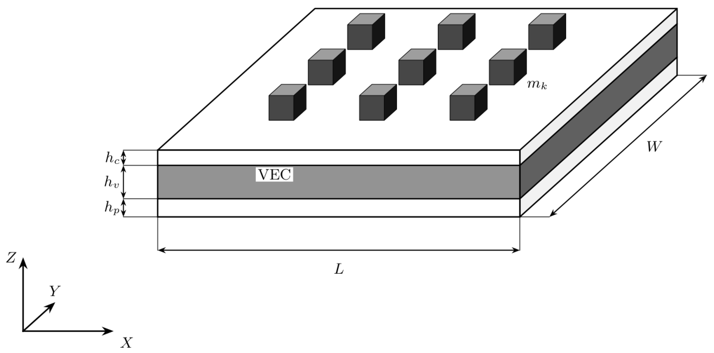
Figure 2.
Sandwich stack with unequal, periodically modulated faces (top thinner, longer wave; bottom thicker, shorter wave). The core thickness is constant. Dashed lines: face and core mid-planes. This section is the X–Z plane. Y points out of the page, so remains the right-handed triad of Figure 1. The horizontal axis drawn here is the local element coordinate x, parallel to X.
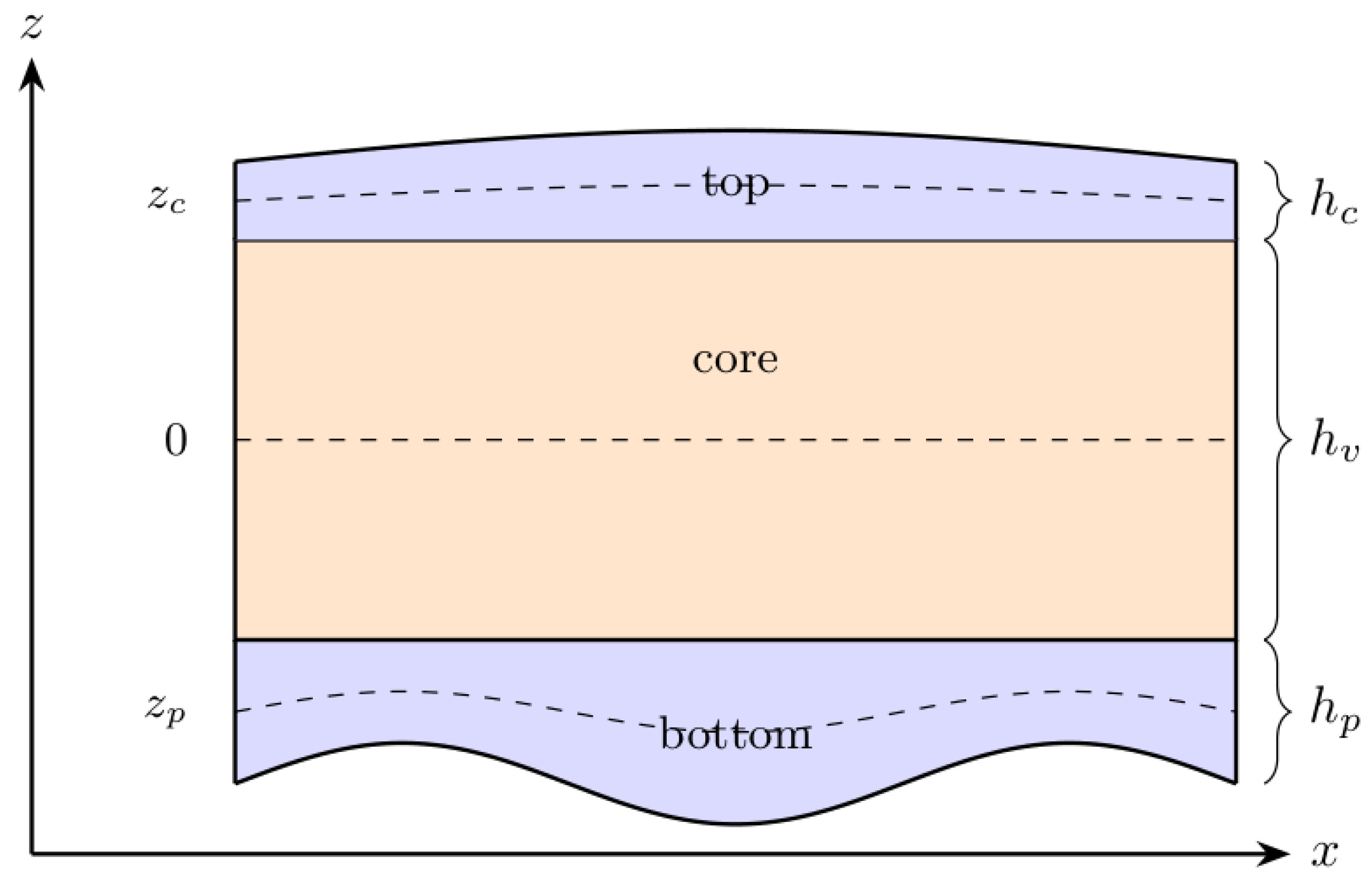
Figure 3.
Normalised field f in (6) for two isotropic wavenumber pairs. (a) Long-wave modulation (). (b) Four half-waves in each direction (). Darker colour denotes a larger local value.
Figure 3.
Normalised field f in (6) for two isotropic wavenumber pairs. (a) Long-wave modulation (). (b) Four half-waves in each direction (). Darker colour denotes a larger local value.
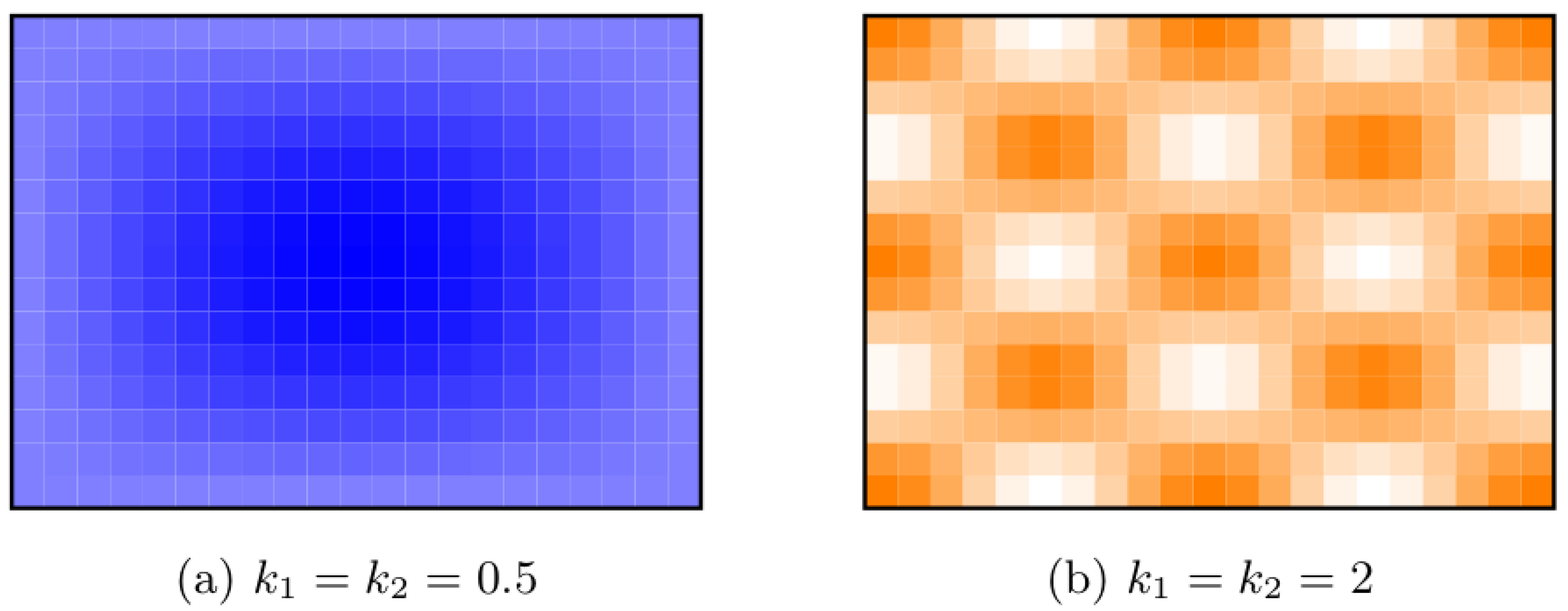
Figure 4.
Galerkin verification of the finite-element FRF on two single-mass plates (, , , symmetric faces). Solid lines: FEM. Markers: Navier–Galerkin series (31). Blue: cosine-modulated faces and core (FEM ). Red: the corresponding uniform plate (). On the modulated plate the Galerkin series peaks at .
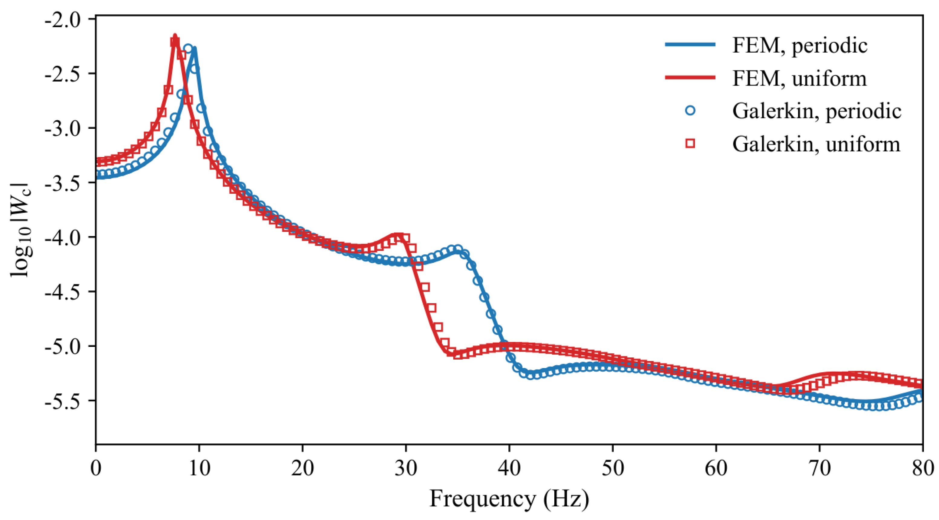
Figure 5.
Centre-point FRFs for varying core wavenumber and thickness.
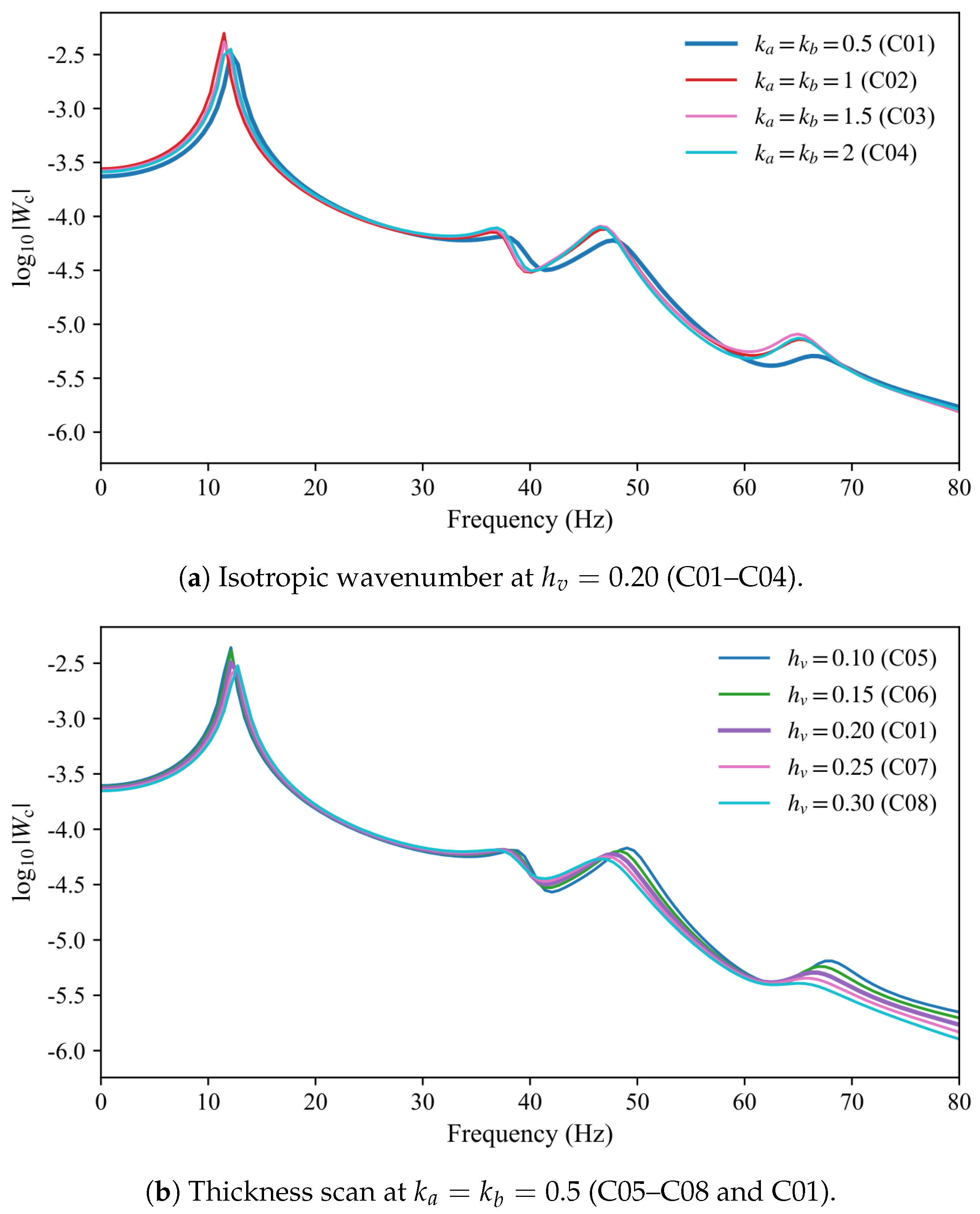
Figure 6.
Centre-point FRFs that isolate the area-averaged core modulus. C09: uniform high-modulus core (). C01: two-dimensional modulation with . C10 and C11: one-dimensional stripes.
Figure 6.
Centre-point FRFs that isolate the area-averaged core modulus. C09: uniform high-modulus core (). C01: two-dimensional modulation with . C10 and C11: one-dimensional stripes.
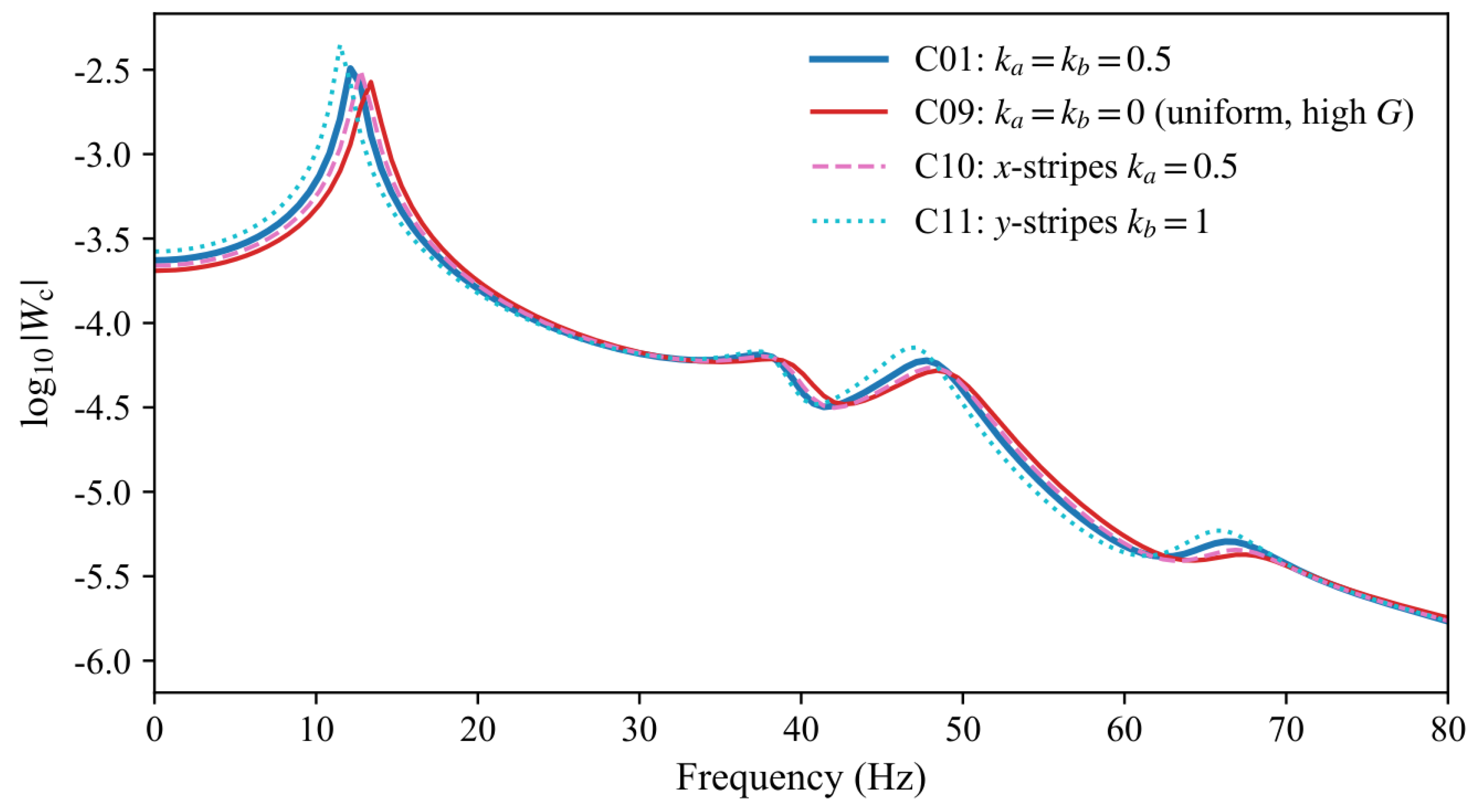
Figure 7.
Centre-point FRFs for face-thickness modulation.
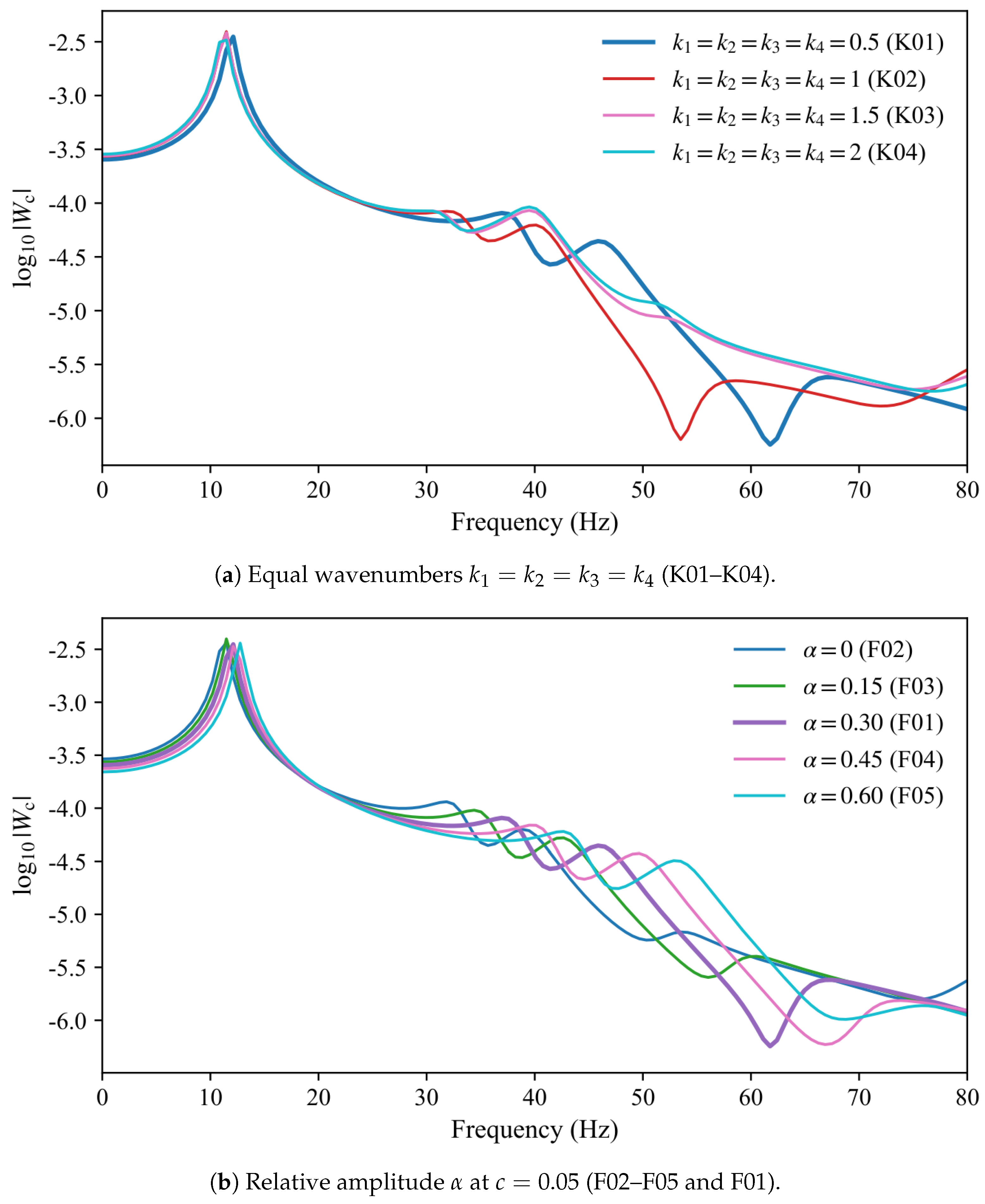
Figure 8.
Centre-point FRFs when are not all equal. Tuples are .
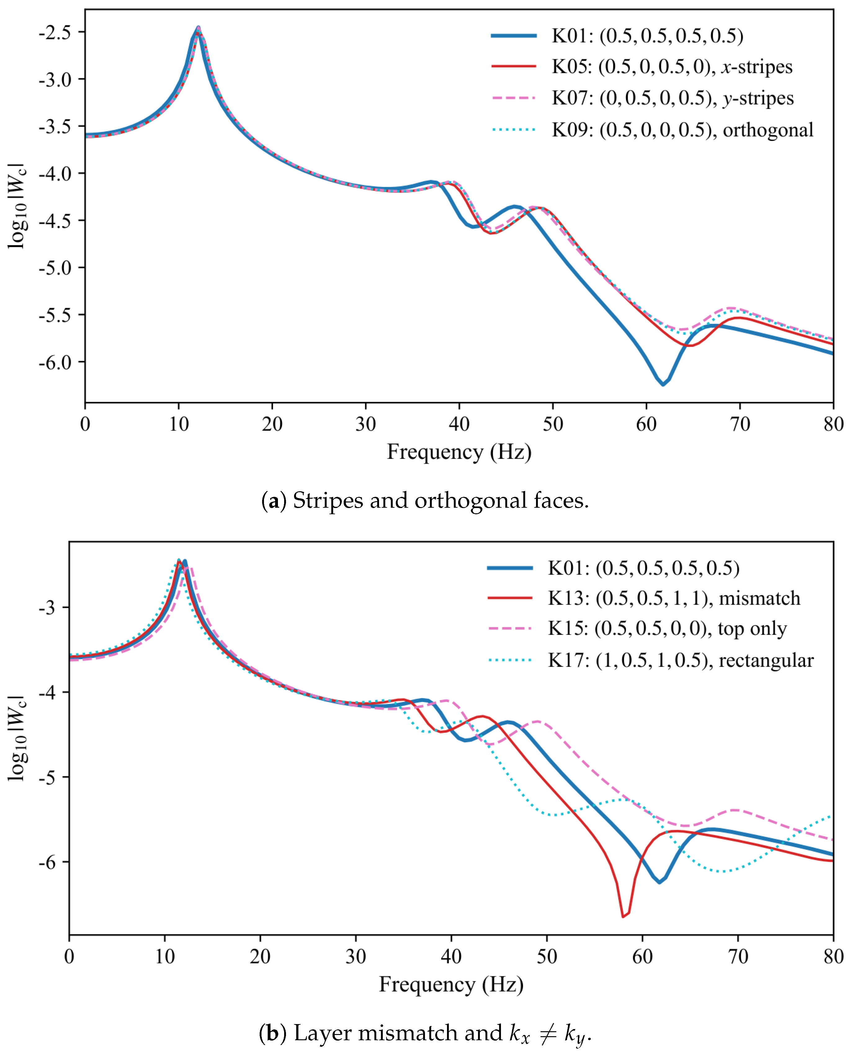
Figure 9.
Centre-point FRFs for face-thickness modulation at and . F10 and F11 overlie each other.
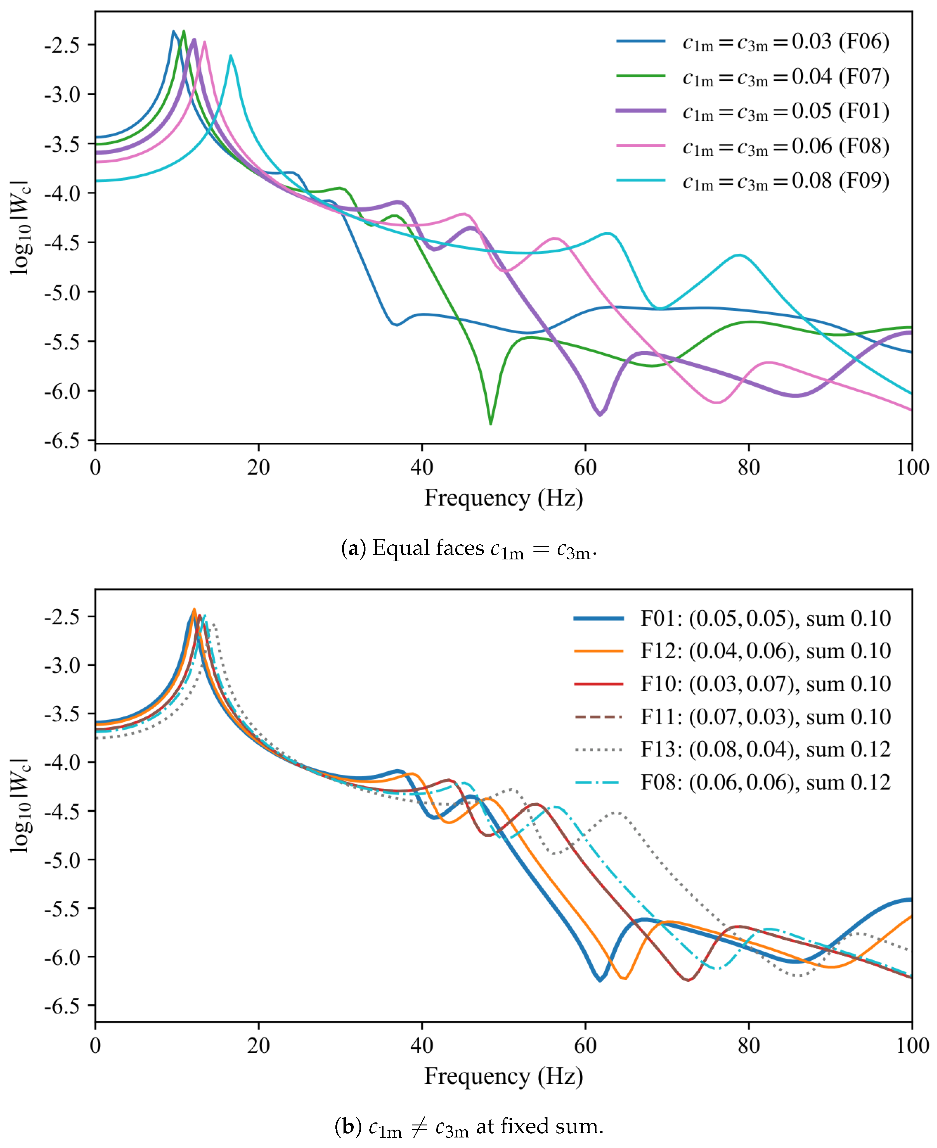
Figure 10.
Centre-point FRFs for the mass-layout archive on the core-C01 plate. D01 is the equal reference of Table 5.
Figure 10.
Centre-point FRFs for the mass-layout archive on the core-C01 plate. D01 is the equal reference of Table 5.
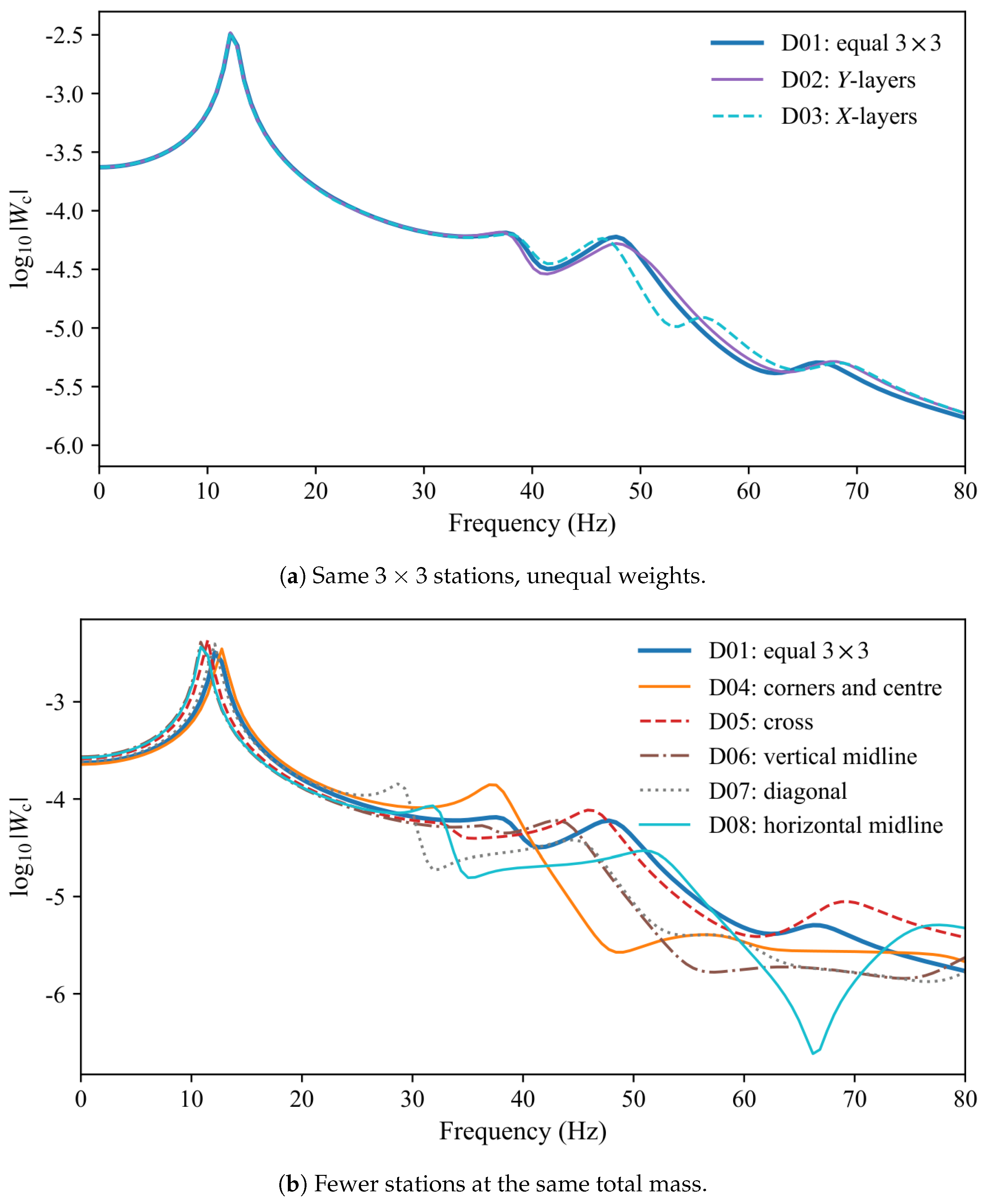
Table 1.
Locked data for the primary campaigns (nine point masses). SI units (metre, kilogram, second): lengths in , moduli in , Kelvin–Voigt viscosities in , densities in . The face row is a stiff isotropic polymer composite. The core row is a soft viscoelastic polymer. The core Young’s modulus changes the reported spectra only negligibly and is set to zero. Neither row is a commercial trade name.
| Quantity | Value |
|---|---|
| Planform | |
| Face E, , | , , |
| Core , | , 0 |
| Core mean , | , |
| Core amplitudes | , |
| Base acceleration | |
| Attached-mass total |
Table 2.
First three centre-point peaks for varying core wavenumber and thickness. Frequencies are grid values (). at .
Table 2.
First three centre-point peaks for varying core wavenumber and thickness. Frequencies are grid values (). at .
| Case | |||||||
|---|---|---|---|---|---|---|---|
| I: isotropic , | |||||||
| C01 | |||||||
| C02 | |||||||
| C03 | |||||||
| C04 | |||||||
| II: thickness at | |||||||
| C05 | |||||||
| C06 | |||||||
| C07 | |||||||
| C08 | |||||||
| III: uniform core and one-dimensional stripes | |||||||
| C09 | |||||||
| C10 | |||||||
| C11 | |||||||
Table 3.
Face-wavenumber peaks at locked and . modulate in X and Y; modulate . Frequencies are grid values; .
Table 3.
Face-wavenumber peaks at locked and . modulate in X and Y; modulate . Frequencies are grid values; .
| Case | ||||||||||
|---|---|---|---|---|---|---|---|---|---|---|
| I: | ||||||||||
| K01 | ||||||||||
| K02 | 1 | 1 | 1 | 1 | ||||||
| K03 | ||||||||||
| K04 | 2 | 2 | 2 | 2 | ||||||
| II: aligned one-dimensional stripes | ||||||||||
| K05 | 0 | 0 | ||||||||
| K06 | 1 | 0 | 1 | 0 | ||||||
| K07 | 0 | 0 | ||||||||
| K08 | 0 | 1 | 0 | 1 | ||||||
| III: orthogonal top and bottom | ||||||||||
| K09 | 0 | 0 | ||||||||
| K10 | 0 | 0 | ||||||||
| K11 | 1 | 0 | 0 | 1 | ||||||
| K12 | 0 | 0 | 1 | |||||||
| IV: top–bottom mismatch | ||||||||||
| K13 | 1 | 1 | ||||||||
| K14 | 1 | 1 | ||||||||
| K15 | 0 | 0 | ||||||||
| K16 | 0 | 0 | ||||||||
| V: rectangular cells, | ||||||||||
| K17 | 1 | 1 | ||||||||
| K18 | 1 | 1 | ||||||||
| K19 | 2 | 2 | ||||||||
| K20 | 2 | 2 | ||||||||
Table 4.
Face amplitude and mean-thickness peaks at . . F01 is the same plate as K01. Frequencies are grid values; .
Table 4.
Face amplitude and mean-thickness peaks at . . F01 is the same plate as K01. Frequencies are grid values; .
| Case | |||||||||
|---|---|---|---|---|---|---|---|---|---|
| Amplitude, | |||||||||
| F01 | |||||||||
| F02 | 0 | ||||||||
| F03 | |||||||||
| F04 | |||||||||
| F05 | |||||||||
| Equal faces , | |||||||||
| F06 | |||||||||
| F07 | |||||||||
| F08 | |||||||||
| F09 | |||||||||
| Unequal faces , | |||||||||
| F10 | |||||||||
| F11 | |||||||||
| F12 | |||||||||
| F13 | |||||||||
Disclaimer/Publisher’s Note: The statements, opinions and data contained in all publications are solely those of the individual author(s) and contributor(s) and not of MDPI and/or the editor(s). MDPI and/or the editor(s) disclaim responsibility for any injury to people or property resulting from any ideas, methods, instructions or products referred to in the content. |
© 2026 by the authors. Licensee MDPI, Basel, Switzerland. This article is an open access article distributed under the terms and conditions of the Creative Commons Attribution (CC BY) license (http://creativecommons.org/licenses/by/4.0/).
Copyright: This open access article is published under a Creative Commons CC BY 4.0 license, which permit the free download, distribution, and reuse, provided that the author and preprint are cited in any reuse.