
Submitted:
09 October 2026
Posted:
10 October 2026
You are already at the latest version
Abstract
Electric bus operators must limit charging-infrastructure investment while supplying enough layover energy to preserve battery reserves during service. Climate changes both energy demand and charging acceptance, linking forecasts to control and infrastructure selection. We propose a scientific machine learning (SciML) framework for climate-adaptive co-design that predicts bus energy from an equipment-based physical prior and multimodal residual learning. Day-level calibration converts forecasts into upper energies that determine inventory targets and charging-window commitments; linear-programming screening is followed by closed-loop qualification of site sets. Public weather and reconstructed Montréal and Singapore duties drive continuous-year simulation with one vehicle configuration. With 28 target fitting days plus 40 calibration days, Singapore-to-Montréal transfer lowers 2025 forecast error by 5.4% against full fine-tuning and 18.7% against gradient boosting. Removing the physical prior and route-network inputs raises error 2.3 to 3.0 times. In 2025, reverse transfer lowers error by 58.0% against the calibrated physical prior and remains 11.3% above gradient boosting. Prediction accuracy and reserve outcomes rank the frozen predictors differently. On Singapore's eight-site design under fixed control in 2025, gradient boosting has the lowest forecast error but 135.03 lost days per operating seed, compared with 9.80 for transfer and 0.43 for the calibrated physical prior. Lost days count failures beyond a forecast-free full-site Reference plus uncommitted dates. Predictor-specific control pairing lowers transfer's lost days from 9.80 to 0.30. In Montréal, qualification restores the terminal needed on the coldest development day. The qualified eight-site predictive design lowers annual charging-subsystem cost by 28.2% against the full-site Reference.
Keywords:
battery-electric buses
; scientific machine learning
; transfer learning
; supervisory charging control
; charging infrastructure co-design
; climate adaptation
1. Introduction
Electrifying city bus fleets links urban transport decarbonisation to long-term decisions about battery capacity and charging infrastructure. For transit operators, the transition must preserve scheduled service while keeping vehicle and charging-system costs affordable [1,2]. Bus duties follow prescribed routes and departure times, so energy replenishment must fit within the charging opportunities available during service. Opportunity charging uses short terminal layovers to replenish the battery, allowing full-day operation with a battery smaller than the duty’s total energy demand [3]. This arrangement makes service continuity depend on where charging is available and how the controller uses each window. The controller must leave the bus with sufficient stored energy for subsequent service while preserving its reserve. A charging plan must therefore match energy delivery to the timing and location of individual duties. Site investment determines charging availability and installed power, while supervisory control determines charging targets and the use of future charging opportunities. Planning consequently needs to couple infrastructure and control around the energy each duty requires and the energy its layovers can deliver. At the wider electric-vehicle network scale, coupled energy–transport planning includes cost, resilience and connectivity objectives [4].
Climate changes both sides of the charging balance. Cold operation increases cabin and battery heating demand [5]. Cabin HVAC also adds cooling loads [6] and humidity control [7]. Low battery temperature also reduces charging acceptance [8]. Measurements from Montréal show seasonal differences in bus energy consumption [9], and regional planning studies select different battery and charger configurations across cities [10]. The energy that must be replenished and the time-dependent power available for replenishment therefore need a common representation. This coupling gives climate-specific energy information a direct role in charging control and site selection.
Physical bus-energy models provide structured estimates of propulsion and auxiliary demand [11,12]. Hybrid models combine physical estimates with data-driven prediction [7,13]. Scientific machine learning (SciML) incorporates physical knowledge into data-driven representations, model structure or training objectives [14,15]. We use this approach to learn residual corrections to an equipment-based energy prior. Uncertainty-aware bus predictors also provide prediction intervals [16]. Transfer learning offers a way to reuse source-domain information when labelled target data are limited [17,18]. Evidence from Canadian buses also shows the importance of adapting energy models to the receiving system [19]. For a cold and a tropical city, the component mix and duty histories differ. Evaluating both transfer directions therefore helps determine which information carries across systems and how much target fitting and calibration contribute.
A forecast enters this decision through the charging supervisor. The supervisor needs an energy requirement that includes the reserve and the future demand that available charging windows must cover. Decision-focused studies motivate evaluating forecasts through their operating consequences [20,21]. Risk-aware microgrid operation similarly trains price forecasts against risk-weighted decision losses induced by forecast errors [22]. Calibrated forecasts already support control of electric-vehicle charging hubs [23], and temperature-dependent reserve rules support bus dispatch [24]. Split-conformal calibration provides an upper-energy estimate with stated coverage conditions [25,26,27]. For opportunity charging, the next step is to translate that estimate into required inventory and commitments within finite windows. Forecast error, calibrated upper energy and the reserve outcomes of the executing controller then describe different aspects of performance.
Infrastructure feasibility depends on the same executing controller. Integrated charger planning and rolling-horizon scheduling connect investment to operation [28], while uncertainty-aware formulations represent variable energy demand in charging and scheduling decisions [29,30]. Data-driven robust planning for residential electric-vehicle car parks jointly determines charger and main-switchboard capacities under uncertain charging demand [31]. Simulation can evaluate charging infrastructure and the operation that uses it [32,33]. Controller-model fidelity also changes planning decisions for electric-vehicle charging sites [34]. The closest studies compared in Table 1 address regional sizing, demand uncertainty, calibrated control or integrated scheduling. The present study connects these decision stages through SciML bus-energy transfer, calibrated inventory requirements and closed-loop acceptance of charging-site sets across climates. This connection allows the same forecast information to be followed from an energy estimate to a charging action and then to an infrastructure outcome.
We develop a SciML-based climate-adaptive co-design framework around this forecast-to-control connection. An equipment-based, component-level physical prior is corrected by supervised residual learning from weather, operating-history and route-network representations. Target adaptation and day-level calibration convert the forecast into upper energies. The supervisor uses these energies to set reserve inventory and backward charging-window commitments. A linear programme (LP) screens the resources offered by each site set, and closed-loop qualification tests its operation with the selected controller and dispatch. The accepted design is evaluated over continuous years with overnight recovery and annual metering.
The evaluation uses public weather and six reconstructed full-day duties in each of Montréal and Singapore, with one common vehicle configuration. Differences between the two cases reflect climate and duty structure. Climate-adaptive design here means that city-specific forecast adaptation and calibration inform the selection and qualification of the supervisor and site set. We evaluate the direction and target-data dependence of transfer, the relationship between forecast information and reserve outcomes, and the charging resources that bind during infrastructure qualification. Annual lost days count failed dates beyond the forecast-free full-site Reference and dates left uncommitted after stranding.
The main contributions of this study are as follows:
- (1)
- We develop a SciML forecast-to-control interface that connects an equipment-based bus-energy prior and multimodal residual transfer to day-level calibrated upper energies, required inventory and backward commitments within charging windows. At 28 target fitting days plus 40 calibration days, Singapore-to-Montréal transfer lowers 2025 error by 5.4% against the closest baseline, full fine-tuning. At the same budget in 2025, reverse transfer improves on target-only learning while gradient boosting remains more accurate.
- (2)
- We evaluate the SciML predictor and its comparators through both forecast accuracy and the operational consequences of predictor–controller pairing. Fixed-control comparisons follow five frozen predictors through inventory decisions to annual reserve outcomes. The calibrated physical prior records the lowest lost days under the fixed Singapore controller. Separately, pairing the anchored transfer variant with its own controller and dispatch reaches 0.30 lost days per operating seed in 2025, against 0.07 for forecast-free dispatch on the same eight sites. These comparisons distinguish forecast accuracy from the performance of the complete pairing.
- (3)
- We develop a closed-loop infrastructure qualification procedure that tests site sets admitted by the LP resource screen under executed control and evaluates the resulting designs over continuous years. In Montréal, qualification adds the terminal required on the coldest development day. The qualified eight-site predictive design has 28.2% lower annual charging-subsystem cost than the twelve-site Reference. At the common 245 kW battery acceptance, charging acceptance and cabin load govern the examined Singapore resource limits, while terminal location governs Montréal’s coldest-day qualification.
2. Methods
2.1. Problem Formulation and Overall Framework
We study the joint selection of charging infrastructure and control for prescribed electric-bus duties through a scientific machine learning (SciML)-based framework. An equipment-based physical prior and supervised residual learning supply the energy forecasts used in this selection. The given inputs are the routes, departure times and terminal layovers, candidate charging terminals, weather records, and vehicle and equipment parameters. A feasible operating case completes the scheduled duties while meeting the registered battery-reserve and cabin-comfort criteria. Terminal locations and finite layover durations determine where and when the fleet can replenish energy before subsequent service.
Co-design selects the active site set S, the common site AC level G, an inventory supervisor and a dispatch policy within prescribed finite candidate domains. Port counts follow maximum scheduled concurrency. The supervisor settings determine the forecast horizon, baseline inventory and credit assigned to future charging windows, while dispatch determines the charging-power request within a layover. A lane combines a design, supervisor and dispatch policy. The learned predictors are fitted by supervised prediction loss before infrastructure and control selection. Each predictive arm then supplies a fixed predictor and calibration margin during design selection.
The co-design framework links SciML energy forecasts to statistical calibration, inventory control and infrastructure selection. The physical plant determines climate-dependent demand and state-dependent charging acceptance. At a layover, causal prediction inputs yield the energy forecasts of complete future decision groups. Day-group calibration converts these forecasts into upper energies, which the supervisor uses to set required inventory and a charge target. Window-budget dispatch also issues group-endpoint and total-energy commitments through backward planning. Charging execution resolves these requests against port allocation, site AC capacity, battery acceptance and the remaining window. In the infrastructure procedure, an LP first screens hardware against fully served reference loads; closed-loop qualification then evaluates the surviving candidate lanes with the executing predictor, supervisor and dispatch. Selected identities remain fixed during continuous-year evaluation.
For each frozen calibrated predictor, staged co-design seeks the lowest-cost passing lane within its prescribed candidate domain:
where A is the annual asset cost (Equation 9), the energy price, and the mean daytime grid energy over the ranking dates . The condition requires zero shortfall within the registered tolerance of the relaxed LP screen. The condition requires full service and compliance with the registered reserve and comfort criteria under the executing supervisor and dispatch. The selection cost combines annual assets with annualised ranking-date daytime energy. Annual evaluation measures J (Equation 14) from assets, complete service-cycle AC energy including overnight recovery, and monthly metered demand charges.
2.2. Cities, Duties and Scenario Inputs
Montréal provides the cold case and Singapore the hot-humid case, with 12 and 9 candidate opportunity-charging terminals (Table 2). The study is a public-data-driven simulation. Hourly NASA POWER data [45] provide temperature, relative humidity, wind, irradiance and precipitation for 2019 to 2025. POWER takes its meteorological variables from the MERRA-2 reanalysis [46] and its irradiance from CERES SYN1deg. The query points are N, W for Montréal and N, E for Singapore (Hourly API v2.10.2, retrieved on 22 September 2026).
Six full-day duties per city are reconstructed from published transport information. Montréal duties link trips in the General Transit Feed Specification (GTFS) snapshot of the Société de transport de Montréal (STM) dated 16 August 2026. Consecutive trips connect at identical stops with layovers of at most 90 minutes, preserving the scheduled GTFS times. Singapore duties follow the SimplyGo stop order and cumulative distance, with a driving speed of 22 km/h, a stop dwell of 20 s and a terminal layover of 10 min. Off-service events connect each duty to a depot at its initial terminal. These fixed timetable snapshots define the networks operated under the historical weather records.
One engineering configuration of vehicle, cabin and electrical equipment serves both cities, so the case differences reflect climate and duty structure. Passenger and traction variation are engineering-scenario draws fixed by the operating seed and shared across compared cases. The plant uses realised weather and these draws to generate demand. Prediction uses the published schedule, completed observations and a causal weather reconstruction, as specified in Section 2.4. Each hourly weather observation becomes available at the end of its hour. Table 2 summarises the weather and reconstructed duties, and Table 3 reports the common equipment parameters and their evidence classes.
2.3. Physical Plant and Energy Labels
The same plant generates the learning labels and executes charging in both cities. It resolves traction, cabin sensible and latent conditioning, reheat, fans, battery thermal management and other auxiliary loads (Table 3). The usable battery capacity is kWh, with a reserve SoC of 0.15, a departure and maximum SoC of 0.95, and charging and discharging efficiencies . Opportunity chargers have a 450 kW DC rating and an AC-to-DC efficiency of 0.92. Depot recovery provides 150 kW of AC and DC intake per vehicle.
Cabin heat and moisture evolve through shell and ventilation exchange, solar gain, passengers, door openings, HVAC delivery and condensation. Heating and cooling set points are 20 and 24 °C, with a 60% humidity set point; comfort spans 18 to 26 °C and relative humidity up to 65%. Cooling dehumidifies with an apparatus dew point capped at 13 °C and reheats the supply air. Delivered heating, cooling and reheat capacities are 32, 35 and 20 kW. Heating and cooling electricity follow temperature-dependent coefficients of performance, while reheat and fan loads enter the same DC-bus demand. Full thermal and moisture equations are given in Section S2.
Actual replenishment depends on supply, concurrent loads and battery acceptance. The connected DC supply is
where is the AC power allocated to the vehicle. Battery acceptance before storage efficiency is
Here E is stored energy, battery temperature and the base charging-rate coefficient. The acceptance plateau is 245 kW. The SoC multiplier is 1 below 0.80, 0.5 from 0.80 to 0.90, 0.25 from 0.90 to 0.95, and zero at the upper limit. The temperature multiplier rises linearly from zero at °C to one at 15 °C, stays at one up to 35 °C, and falls to zero at 55 °C. When supply covers the requested DC-bus load , the stored charging power is ; otherwise the stored-energy discharge rate is . Finite windows, shared site capacity and evolving battery state therefore determine the energy delivered by each charging request.
A decision group contains consecutive operating events through the next layover, inclusive. At the preceding layover, a query forecasts one complete future group beginning within six hours in the learning study; each such query is a forecast event. The component label is the requested DC-bus energy over that group, expressed as stored-battery discharge-equivalent energy:
where is in kW and t in hours, so is in kWh. Labels use realised weather and scenario forcing, while the predictor receives the causal information specified in Section 2.4. Label generation uses a 24-hour warm-up and 60 minutes of preparation before departure. Passenger and traction variation are fixed by the operating seed and shared across compared cases.
Exact exponential relaxation advances the coupled states in steps of at most 10 s. Conservation records close the electrical, cabin-heat, water and battery-heat balances, and annual metered energy reconciles with cycle energy within kWh. Batched FP64 integration on the GPU generates all labels. Independent validation addresses the corresponding physical chains (Section S2). EnergyPlus 25.2.0 [49] reproduces daily HVAC electricity in four aligned cases within 4.8% against a 10% criterion, latent energy within 2.4% against 15%, and relative humidity within 1.3 percentage points against 5 percentage points. OpenModelica 1.27.0 [50] reproduces grid energy in three coupled charging and thermal-management cases within kWh. Halving the time step from 10 to 5 s changes daily energy by at most 0.4%.
Ten measured Zurich trolleybus missions [51] support the temperature dependence of demand. In whole-mission holdouts, mission-energy error is 14.9% for a constant-energy regression, 13.3% with mechanical power, and 5.8% after adding temperature. These measured-data regressions and independent solver comparisons support the model mechanisms; the Montréal and Singapore labels and closed-loop trajectories are generated by the common plant.
2.4. SciML Energy Prediction and Cross-Climate Adaptation
The SciML energy predictor combines an equipment-based physical prior with supervised residual corrections [14,15].
The predictor estimates stored-battery discharge-equivalent energy for each complete future decision group. Its inputs comprise 24 completed hourly weather rows of five channels, six forecast hours, 60 completed minutes of 12 operating variables with availability masks, and an eight-node directed path. Each hourly observation becomes available at the end of its hour. The causal weather forecast repeats the previous day’s values at the same clock hour. The eight-component physical prior evaluates the equipment maps using this forecast and the observed mean occupancy.
Three convolutional sequence encoders summarise weather history, forecast weather and masked operations. A two-layer graph encoder summarises the directed path. Their four 64-value summaries and the eight-component prior enter a 264-input fusion head. A zero-initialised correction layer predicts a scaled residual about the prior,
where is the prior energy, its component scale from the fitting period, the network output and . The untrained network reproduces the prior. The loss adds the mean squared, scale-normalised component errors to the corresponding mean squared total-energy error. The predictor’s physical structure enters through the equipment prior, component decomposition and nonnegative outputs.
The network has 43,656 parameters. Partial adaptation [17] updates 27,080 parameters in the operations encoder, fusion head and correction layer, with the weather-history, forecast and graph encoders frozen. Source training uses Adam [52], learning rate , batches of 256 and at most 200 epochs. Early stopping uses 24 source-city development days of 2022, patience 20 and restoration of the best state. Adaptation runs 80 epochs at . With probability 0.5, training masks either the most recent 1 to 60 operating minutes or a random 0 to 30% of minutes; the prior keeps its full-information value. Training and inference use FP32 on the GPU.
The anchored transfer variant re-estimates input statistics and component scales from the unlabelled inputs of the full 2019 to 2021 target fitting calendar: 1,094 Montréal or 1,093 Singapore days. The source-coordinate variant keeps source normalisation. Directional selection uses mean daily MAE on the target city’s 2022 development queries at 28 fitting days, averaged over three seeds and five subsets. Montréal-to-Singapore selects source coordinates (1.493 versus 1.695 kWh); Singapore-to-Montréal selects anchoring (0.960 versus 0.998 kWh).
Ten comparator arms comprise the physical prior, affine recalibration, source-only prediction, target-calibrated source prediction, source re-anchoring, HGB, target-only training, early fusion, pooled learning and full fine-tuning. HGB [53] uses the scikit-learn histogram implementation [54], with 200 iterations, learning rate 0.05 and 31 leaves. It regresses the total-energy residual on the flattened inputs and prior. Both the neural model and HGB therefore use the equipment-based prior, with component-wise and total-energy residual learning, respectively. Supplementary Material, Section S3, gives layer dimensions, normalisation rules, arm-specific data access and the complete training loss.
2.5. Day-Level Calibration and Forecast Interface
The statistical forecast interface uses split-conformal calibration [25,26,27] to convert each point forecast into an upper energy. For month-stratified calibration days of 2023, the day score is the largest positive residual among that day’s forecast events. The margin is the score of rank :
With and , , so m equals the largest day score. For an exchangeable new day, the nominal simultaneous coverage of all forecast events is 0.975. Calibration uses target-city days for all arms except source-only prediction, which uses source-city days. Measured simultaneous-day coverage is reported separately for 2024 and 2025. Each frozen predictor keeps its calibrated margin constant throughout annual execution; the inventory supervisor receives the upper energy for each complete future decision group.
Fitting and calibration use separate labelled dates. A 28-day arm uses 28 target fitting days and 40 target calibration days, totalling 68 labelled target days. Anchored variants also access the unlabelled target fitting inputs; source-trained arms add source fitting labels and the 24 source development days. Annual deployment uses one frozen fit per learned arm, with model seed 101 and target-day sample 0 at the arm-specific budget defined in Section 2.9.
2.6. Inventory Supervision and Daytime Charging Dispatch
The inventory supervisor applies the calibrated upper energies to the prescribed horizon and charging-credit rule. At a layover decision time , the supervisor collects the complete future decision groups that start before and orders them by their end times. Each group includes its final layover. The calibrated upper energies give the cumulative requirement . Published future charging windows that end by the start of group g provide the stored-energy credit . The credit combines reachable DC power, window duration, charging efficiency and a 2 kW layover auxiliary allowance. The required inventory R, capacity-capped target and saturation shortfall are
Here C is battery capacity, the baseline inventory fraction and the fraction of future charging credit used by the supervisor. A decision is saturated when . Eight controllers span min, and . Controllers 5, 6 and 7 define the annual roles, with of , and . The target specifies desired stored energy; the available window, port allocation and state-dependent acceptance determine the energy attained.
Ports are allocated by arrival time and then vehicle identifier. A dispatch policy sets the requested DC power . The vehicle takes at most , where is the last observed auxiliary power, initially 2 kW. Site AC headroom is allocated in the same arrival order as . Remaining-window dispatch spreads the stored-energy target deficit over the remaining layover, accounts for charging efficiency, adds auxiliary power and caps the request at the charger rating. Maximum-inventory dispatch requests the full DC rating throughout every layover and is the forecast-free daytime reference.
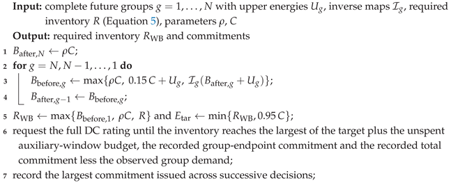
Window-budget dispatch plans backwards from the final post-group floor (Algorithm 1):
The inverse returns the starting stored energy needed for zero-load charging over the available segments of group g to reach its argument. It includes SoC taper, residual site capacity under the scheduled queue and the decision-time battery-temperature multiplier. The backward update passes each before-group requirement to the preceding group’s after-group requirement. The final target is .
Across successive decisions, the planner retains the largest issued endpoint commitment and total commitment , corresponding to and . Let be the delivered group demand in stored-battery discharge-equivalent kWh and the unspent equipment-envelope auxiliary budget of the current window. The command threshold is
Window-budget dispatch requests the full DC rating while and auxiliary power, capped at the rating, afterwards. The detailed plant executes the evolving loads, acceptance and allocation. Inventory requirements, targets, command thresholds and delivered energy therefore have distinct roles. The auxiliary envelope and inverse-map construction are specified in Section S4 of the supplement.
| Algorithm 1: Backward window planning at one layover |
 |
2.7. Infrastructure Screening and Closed-Loop Qualification
A design is a nonempty candidate-terminal subset S with a common site AC level kW. Each active site receives ports equal to its maximum scheduled concurrency. Annual asset cost and annualised unit cost are
Here is installed capital, the real discount rate, T asset life and the maintenance fraction. Capital is CAD 1448823.53 per opportunity port and CAD 301.84 per kW of grid capacity, after consumer-price normalisation and a 20% project allowance (Table 3). Port and grid lives are 15 and 30 years, with maintenance fractions of 0.01 and 0. A one-port site at 300 kW costs CAD 150033.62 annually. Depot capital is common across designs; depot energy and demand charges enter annual operating cost.
Resource screening uses a perfect-information LP independently of the predictive controller. The screen evaluates hardware using fully served reference loads; closed-loop qualification evaluates the resource-feasible designs with the executing predictor and control pairing. A development-date reference runs all sites at 300 kW with controller 7 and maximum-inventory dispatch on the scalar CPU executor, which allocates the raw power request. Its cabin-HVAC trajectory enters the LP when all vehicles and HVAC demand are fully served. The LP combines this trajectory with known traction and hotel loads on an event-aligned clock. Charging opportunities comprise published layovers at installed sites and vehicle depot stays; time-dependent battery thermal-management demand belongs to the detailed plant. For vehicle v, charger j and slot t,
Here is starting stored energy, q charger DC supply, DC energy entering the battery, DC energy supplied by the battery, z unmet load and D requested DC load. All flows are kWh per slot. The LP uses the flat 245 kW acceptance plateau, site AC capacity and fractional port occupancy, with initial energy . It minimises , subject to and terminal restoration , where is terminal energy shortfall and h is the number of slots in the day. Known demand, fixed cabin demand, fractional sharing and a perfect scheduler define the relaxation. An optimum above kWh certifies resource infeasibility; zero shortfall admits the design to closed-loop qualification.
Dates with positive shortfall for all sites at 600 kW receive deficit certificates and leave the ranking population. A monotone cost-ordered search tests 625 Montréal and 32 Singapore designs at 245 kW acceptance within the prescribed domains and . The original search forms a frontier of the two cheapest LP-feasible 300 kW designs per site count.
For a frozen predictor, a lane combines a design, controller and dispatch policy. Original qualification evaluates frontier designs and the all-site reference with the eight controllers and two predictive dispatch policies, alongside the controller-7 maximum-inventory lane. The 26 Montréal and 25 Singapore ranking dates run hardest first from full departure states. A lane passes every date with full service, zero stranding and reserve violation, and temperature and humidity violation fractions at most 0.01 of occupied vehicle-seconds.
The registered selection minimises annual assets plus among passing lanes, where is mean daytime grid energy on the ranking dates. A subsequent development-stage amendment screens the complete Montréal LP-feasible 300 kW domain: all 72 subsets first run with controller 7 and maximum-inventory dispatch; the 16 passing subsets below ten sites then run with the anchored 28-day transfer model, all eight controllers and both predictive policies. Algorithm 2 records both search scopes. Selected identities are fixed before annual execution, which evaluates complete service cycles, continuous overnight recovery and metered demand charges.
| Algorithm 2: Staged infrastructure selection |
| Input: duties, development weather, equipment parameters, frozen predictors, candidate sites, grid levels, controllers and dispatch policies |
| Output: selected design, controller and dispatch, annual reliability and cost |
|
2.8. Continuous-Year Operation and Cost Accounting
All annual roles use the same rolling depot-recovery policy. A service cycle runs from the first departure of one day to the first departure of the next. A three-stage lexicographic mixed-integer linear programme (MILP) replans every 15 minutes and at departure-related events, then executes the first planned slot. Its objectives minimise departure energy shortfall, early-recovery shortfall, and finally energy and monthly peak cost, in that order. The programme includes 90 minutes of cabin preparation and reserves shared port, DC and AC capacity during the final 15 minutes before departure. It models port binaries, grid and charger capacities, SoC acceptance bands, auxiliary loads and peaks already metered. HiGHS [55] solves it on the CPU and selects among equal-cost schedules. Night forecasts combine the latest available observation with the previous day’s weather increment. Battery and cabin states, operating histories and monthly metered peaks continue across service cycles.
Annual execution starts with the preceding 31 December as a context cycle. The final recovery night uses a replay of the scored year’s 1 January weather, from midnight to the latest first departure: seven hourly rows in Montréal and six in Singapore. This replay enters the final service cycle’s recovery and energy. Demand billing covers the twelve local civil months and ends at the midnight before the replay. A stranded vehicle stops its case on that operating seed, and subsequent dates remain uncommitted.
Daytime qualification requires full service, zero reserve-violation time, and temperature and humidity violation fractions at most 0.01 of occupied vehicle-seconds. Night restoration requires each vehicle to depart within kWh of , with its cabin inside the comfort band and zero reserve-violation time during the night. A service cycle passes when both conditions hold. The Reference activates all candidate sites at 300 kW with controller 7 and forecast-free maximum-inventory dispatch. Its failed dates define the reference-failure set on each seed. A role is relatively eligible when every date is committed and every failed date also belongs to that Reference set. Lost days count additional failed dates and dates left uncommitted:
where is the failed-date set of role r on seed w, and counts uncommitted dates. Failed-cycle share includes Reference-failure dates and is the absolute failure rate.
The annual charging-subsystem cost combines annual assets, complete service-cycle AC energy and monthly metered peak intake:
where CAD/kWh, CAD/(kW month), includes daytime operation and overnight recovery, and is the mean AC power at meter over a 15-minute interval in billing month b. Meters cover opportunity sites and the depots; vehicle powers at each intake are summed before taking its monthly maximum. The selection cost of Equation 1 uses annualised ranking-date daytime energy, while J measures the continuous-year account. Role-mean annual costs use complete-record seeds, with every service date committed and every intake metered in all twelve local months. Cost contrasts use the operating seeds on which both roles are relatively eligible.
2.9. Evaluation Protocol and Statistical Analysis
Chronological partitions assign 2019 to 2021 to fitting, 2022 to development, 2023 to calibration, 2024 to the first evaluation year and 2025 to the confirmation year (Table 4). The fitting calendars contain 1,094 Montréal and 1,093 Singapore days. Five nested month-stratified subsets at target budgets of 0, 7, 14, 28 and 56 fitting days, with model seeds 101, 202 and 303 in each transfer direction, form 150 direction, budget, subset and seed cells. A 28-day target arm also uses 40 calibration days; anchored variants use the unlabelled target fitting calendar. Development uses 24 prediction days, 26 Montréal co-design dates and 27 Singapore co-design dates, with 25 Singapore ranking dates after two deficit certificates. Learning evaluation covers 364 dates in 2024 and 363 in 2025, from 2 January to 30 December, whereas annual execution covers all 366 and 365 service dates.
Each annual arm uses one frozen predictor, seed 101 and subset 0 at its arm’s budget. The adapted, gradient-boosting and target-only arms use 28 target fitting days, and the physical-prior, source-only and re-anchored arms use 0. Operating seeds are 1000 to 1009 in 2024 and 2000 to 2029 in 2025; stress tests and network-weather crossing use seed 1000.
Choices called registered were fixed in dated registration files before the runs they govern. Montréal weather of 2025 was available during development, and Singapore weather of 2025 became available with the confirmation runs. Original frontier qualification on the 2022 development dates selected the Registered designs on 24 September 2026. Their annual cases ran from 24 September to 27 September, ending at 04:44. Complete-domain Montréal qualification again used the 2022 development dates, submitted on 27 September at 19:22 and running from 19:28 until stage 2 completed at 20:36. The eight-site cases, selection rule and task definition were registered at 20:42, and annual execution of those cases started on 28 September at 05:33. This amendment followed the original annual runs and preceded the annual runs of the eight-site cases. All stated execution times use America/Toronto time (UTC−4). Annual weather consists of the scored year, the preceding 31 December context cycle and the scored year’s 1 January weather replay used to close the final recovery night, as defined in the annual-execution subsection.
Table 5 separates the annual comparisons. Cases of one city and year share weather, schedule, operating seeds, equipment, prices and night recovery. The all-site adaptation comparison holds hardware and control fixed while changing target fitting and calibration. Predictor swaps hold the Registered design, supervisor and dispatch fixed; predictor-specific joint pairing selects a design, supervisor and dispatch for each information arm. Montréal transfer roles use the anchored variant. In Singapore, the Adapted and Registered roles use source coordinates, while the transfer Joint pairing uses the anchored variant. Infrastructure contrasts compare the full-site Reference, the LP-minimum, the Registered design and the separately selected predictive and forecast-free eight-site Montréal designs. The supplementary registry identifies every executed role and year; Singapore’s joint HGB and target-only cases were executed in 2024.
Learning contrasts average the daily mean absolute error (MAE) over the 15 seed-subset fits of an arm and resample seven-day calendar blocks of consecutive dates. HGB has five distinct subset fits because its fit depends on the target-day subset only. Each direction and year forms a family of 32 comparisons, pairing four target budgets with eight comparators: HGB, target-only training, early fusion, pooled learning, full fine-tuning, the two physical-prior variants and the other transfer variant. The three source-model arms are reported in the supplement.
Annual lost-day contrasts resample operating seeds and seven-day blocks, with moving blocks primary and circular and stationary blocks as sensitivity [56,57,58]. Holm adjustment [59] is primary, and Benjamini-Hochberg adjustment [60] is supplementary within each city, year and outcome over distinct role contrasts. Cost contrasts resample the seeds on which both cases are relatively eligible.
Mechanism contrasts average within each seed and date and resample seven-day date blocks with seeds nested. Forecast rows pair on seed, date, vehicle, decision event and predicted event; decisions pair on the first four keys, vehicle-days on the first three, and cycle outcomes on seed and date. The eight primary metrics of the 2025 transfer-HGB comparison form the mechanism Holm family.
All resampling uses 10,000 GPU draws with generator seed 2026, percentile 95% intervals and an add-one two-sided p-value, with a minimum of 2 in 10,001, or 0.0002. Holm factors of 8, 10, 14, 19 and 32 yield floors of 0.0016, 0.0020, 0.0028, 0.0038 and 0.0064. Values at these floors are written “adjusted ”. Margins are constants of the frozen fits, so their differences are point values. Annual and mechanism intervals describe operating-seed and calendar-block variation for these frozen fits.
3. Results
3.1. Climate-Dependent Energy Demand
Climate changes the composition of requested fleet energy under the common vehicle and equipment configuration (Figure 1). In Montréal, non-traction loads account for 18% to 42% of requested energy. Cabin heating contributes 30% to 32% from December to February, while cooling and dehumidification reach 20% in July. In Singapore, non-traction loads account for 39% to 42%, and cooling and dehumidification contribute 34% to 36% in every month. These are the 2025 Reference-design means over 30 operating seeds. The component structure provides the physical basis for the energy prior and the climate-dependent demand used in co-design.
3.2. Cross-Climate SciML Prediction and Forecast Calibration
Anchored transfer lowers Montréal forecast error against the closest baseline. The adapted predictor combines the equipment-based prior with supervised component-wise residual corrections. With 28 target-fitting days plus 40 calibration days, the Singapore-to-Montréal model reaches an MAE of 0.918 kWh per forecast event in 2025 (Figure 2, Table 6). This is 5.4% below full fine-tuning at 0.971 kWh and 18.7% below HGB at 1.129 kWh. The paired difference against HGB is -0.211 kWh (95% interval -0.256 to -0.164). These learning comparisons average the 15 seed-subset fits of each budget. Annual comparisons in the following subsections use one frozen fit per predictor, with seed 101 and subset 0.
The cold-direction gain persists across budgets and both years. At 28 days in 2024, transfer reaches 0.880 versus 1.072 kWh for HGB, a 17.9% reduction, and lowers MAE by 6.0% against full fine-tuning. All 56 contrasts against the seven baselines, across four budgets and two years, favour transfer after Holm adjustment (adjusted ). At 56 days, transfer remains 9.1% below HGB in 2024 and 14.3% below it in 2025. In both years, Singapore-to-Montréal transfer with 7 and 14 target days is more accurate than gradient boosting with 14 and 28 days (Table 6).
Reverse-direction gains depend on the comparator. The 2022 development error selects source-coordinate transfer for Montréal-to-Singapore. It has lower MAE than full fine-tuning, pooled learning and both physical-prior variants in all eight budget-year comparisons, and than the target-only network in seven of eight. At 28 days, reductions against target-only training are 4.0% in 2024 and 10.0% in 2025. They are 14.7% and 10.1% against full fine-tuning, and 63.2% and 58.0% against the calibrated physical prior; the largest adjusted p of these six contrasts is 0.0096. HGB and transfer have MAEs of 1.771 and 1.772 kWh at 28 days in 2024. In 2025, transfer has 11.3% higher MAE than HGB at 28 days: 1.843 versus 1.656 kWh. The paired difference is 0.187 kWh (95% interval 0.056 to 0.296), with adjusted . Transfer is 9.9% to 18.1% above HGB across the four budgets of 2025 (adjusted ). Early fusion is below transfer at 56 days by 0.175 kWh in 2024 and 0.102 kWh in 2025 (Section S6 of the supplement). The transfer and HGB forecasts both use the physical prior; their differences concern the complete forecast methods. Section 3.3 evaluates the frozen predictors through their inventory supervisor.
Full-path withdrawal and learned-branch ablation measure different information dependencies. Both use the anchored transfer model at 28 target days and evaluate the 2024 dates. Network withdrawal removes the graph input and the horizon table read by the prior, setting all eight prior components to zero. After retraining and recalibration, MAE rises from 2.094 to 6.218 kWh in Montréal-to-Singapore and from 0.880 to 2.036 kWh in Singapore-to-Montréal, factors of 2.97 and 2.31. Learned-branch ablation instead keeps the complete prior. With that prior present, the operating-history branch lowers MAE by 25% in Montréal-to-Singapore (2.794 to 2.094 kWh) and by 6% in Singapore-to-Montréal (0.937 to 0.880 kWh). Removing the learned weather or graph branch changes MAE by at most 0.014 kWh (Table S19 of the supplement).
Measured simultaneous-day coverage is below the nominal target in 15 of 16 combinations of predictor, direction and year. At 28 days, coverage of the annual transfer variant, HGB, target-only network and calibrated physical prior spans 0.929 to 0.976 across both directions and both years. This metric requires every forecast event of an evaluation day to lie below its upper energy. The nominal 0.975 coverage applies to exchangeable new days; later-calendar evaluation reports the measured coverage [61]. For the frozen fits used in annual execution, event-level coverage of these four calibrated predictors exceeds 0.989. Day-level and event-level coverage therefore describe different evaluation units and populations.
3.3. Forecast Accuracy and Reserve Reliability Under Fixed Control
The calibrated physical prior gives the lowest lost days under Singapore’s fixed control, while HGB gives the lowest forecast MAE (Figure 3a,c, Table 7). These comparisons use the Registered eight-site design, controller 5 and remaining-window dispatch, with one frozen predictor per arm. In 2025, the physical prior’s margin of 16.220 kWh accompanies 0.43 lost days per operating seed. Source-coordinate transfer, with a margin of 14.362 kWh, records 9.80 lost days; the target-only network (9.821 kWh) records 48.90, HGB (8.735 kWh) 135.03 and source-only prediction (5.535 kWh) 361.43. HGB reaches an MAE of 1.605 kWh per forecast event, against 1.932 for transfer, 2.013 for the target-only network and 4.386 for the physical prior. The 2024 outcomes follow the same reliability order: 0.40, 8.40, 52.80, 123.80 and 356.10 lost days. Source-only prediction is the only arm that strands.
Across these five frozen predictors, the Spearman correlation of lost days is with the margin and 0.10 with MAE in each year. This is a descriptive association among five deployment fits under one control configuration. The two years execute the same fits. The frozen HGB margin of 8.735 kWh is the smallest of its five distinct subset fits, whose margins span 8.735 to 12.771 kWh. The source-coordinate transfer margin of 14.362 kWh ranks tenth of 15 fits, with a range of 8.667 to 15.248 kWh (Section S6 of the supplement). The annual and mechanism intervals describe operating-seed and calendar-block variation for these frozen fits; the margin ranges separately describe variation across the learning fits.
In 2025, transfer lowers lost days by 125.23 days per seed (95% interval 109.33 to 139.37) relative to HGB and by 39.10 days (29.50 to 48.37) relative to the target-only network (adjusted ). The physical prior lowers them by 9.37 days (5.43 to 13.73) relative to transfer. Montréal’s Registered design records zero lost days for every predictor in both years. At 28 target fitting days, transfer reduces the physical prior’s MAE by 58% to 63% in Montréal-to-Singapore and by 40% in Singapore-to-Montréal in the learning study. The fixed-control comparison therefore assesses the transfer predictor’s accuracy gains together with the physical prior’s stronger reserve reliability in Singapore.
The absolute failed-cycle shares follow the same Singapore order (Figure 3d). Transfer fails on 33.8% of the seed-days of 2025, HGB on 68.2% and the target-only network on 44.6%, against 31.2% for the Reference and 31.3% for the physical prior. Lost days count additional failed dates relative to the Reference plus dates left uncommitted; failed-cycle share includes every failed cycle. Under these four predictors, every vehicle completes its duty. Their additional failures are shallow reserve violations. On failed dates that the Reference serves, the mean minimum SoC is 0.134 to 0.139 for transfer, HGB and the target-only network, against the 0.15 reserve.
3.4. From Calibrated Upper Energy to Inventory and Charging Outcomes
Statistical calibration supplies the upper energies used by the inventory supervisor in Equation 5. At Singapore’s Registered design, paired execution connects the upper-energy forecasts to charge targets, end-of-day energy and reserve outcomes (Table S26 of the supplement). Source-coordinate transfer has a margin 5.627 kWh per forecast event wider than HGB. Its mean upper-energy headroom, the upper energy minus actual requested energy averaged over forecast events, is larger by 5.265 kWh. Headroom equals mean forecast bias plus the calibrated margin.
In the 2025 transfer-minus-HGB comparison, required inventory rises by 14.901 kWh per charging decision (95% interval 14.283 to 15.511), and the charge target rises by 14.540 kWh (13.943 to 15.121). Saturated decisions rise by 4.9 percentage points, and end-of-day energy rises by 3.346 kWh per vehicle-day (3.082 to 3.614). Failed-cycle share falls by 34.4 percentage points (−38.1 to −30.0). The comparison pairs 1,248,300 forecast rows over 30 operating seeds, and the five varying endpoints from required inventory to failed-cycle share each have adjusted . The margin difference is a point comparison of two constants. The 2024 execution shows the same signs, with failed-cycle share lower by 31.6 percentage points. Both predictors keep mean upper-energy exceedance below 0.02 kWh per forecast row; the 2025 exceedance difference of 0.010 kWh has an interval spanning zero (adjusted ).
The target-only network follows the same inventory-to-outcome ordering among the three learned predictors. Its margin is 4.541 kWh narrower than transfer’s, its required inventory is 10.482 kWh lower (95% interval 9.912 to 11.058), and its failed-cycle share is 10.8 percentage points higher (8.1 to 13.3). The paired endpoints therefore show how each frozen calibrated forecast enters the executing supervisor under common hardware and control.
The physical prior achieves fewer failures with lower mean headroom and inventory than transfer. Its margin is 1.858 kWh wider, yet it requires 3.477 kWh less inventory per decision (95% interval 2.774 to 4.185) and fails 2.6 percentage points less often (1.5 to 3.8). Its mean forecast bias of −4.04 kWh per forecast event brings mean upper-energy headroom to 12.2 kWh, 1.3 kWh below transfer’s 13.5 kWh. Margin, mean forecast bias and resulting inventory therefore describe different parts of the operating comparison.
Across the three pairings, the required-inventory difference is 2.7 to 2.8 times the headroom difference. With , Equation 5 takes the maximum over the complete horizon; the factor is consistent with the mean of 2.7 groups per decision, shared by all predictors. Mean headroom orders the inventories of these pairings, while the physical prior reaches fewer failures with less inventory. Section S7 reports its forecast tails and late-day upper-energy profile. The late-day summary conditions on seed-days when transfer fails and the physical prior passes and describes the temporal profile of that selected outcome group. Reliability depends on the calibrated forecast profile together with inventory and charging execution.
3.5. Predictor-Specific Controller and Dispatch Pairing
Predictor-specific pairing reduces lost days on Singapore’s eight-site design (Figure 3b, Table 7). In 2024, HGB falls from 123.80 to 1.90 lost days per seed when controller 6 and window-budget dispatch replace controller 5 and remaining-window dispatch on the same hardware. The target-only network falls from 52.80 to 6.70. These two contrasts keep the predictor fixed and change the controller and dispatch. Source-coordinate transfer under fixed control records 8.40 lost days, while anchored transfer with controller 6 and window-budget dispatch reaches 0.30, with seven of ten seeds relatively eligible. The physical prior keeps 0.40, because its selected pairing coincides with fixed control. Among these 2024 pairings, transfer reaches 0.30 lost days, compared with 0.40 for the physical prior, 1.90 for HGB and 6.70 for the target-only network.
The 2025 confirmation reproduces the anchored-transfer pairing result at 0.30 lost days per seed, with 22 of 30 seeds relatively eligible. This is 9.50 days (95% interval 5.50 to 13.93) below the Registered design (adjusted ). The corresponding 2024 reduction is 8.10 days (3.90 to 13.60, adjusted ). This comparison changes the transfer variant, controller and dispatch together: source-coordinate transfer with controller 5 and remaining-window dispatch becomes anchored transfer with controller 6 and window-budget dispatch. The physical-prior pairing records 0.43 lost days in 2025. HGB and target-only joint pairings were executed in 2024; their joint-pairing entries for 2025 remain unexecuted in Table 7.
3.6. Infrastructure Feasibility and Closed-Loop Qualification
LP screening admits seven-site Montréal designs, while closed-loop qualification requires eight sites. At the registered net acceptance of 245 kW, the cost-ordered search tests 625 designs. Of these, 216 pass the LP on all 26 ranking dates. They comprise 72 site subsets at three AC levels. The subsequent complete-domain qualification evaluates the 72 LP-feasible subsets at 300 kW. Montréal’s LP minimum uses 7 of 12 sites. Its annual assets are CAD 1 050 235, compared with CAD 1 800 403 for all sites, a reduction of 41.7%. Singapore’s LP minimum uses 8 of 9 sites at CAD 1 200 269, 11.1% below all sites.
Peel / Sainte-Catherine separates the passing and failing Montréal designs in the forecast-free qualification screen. With controller 7 and maximum-inventory dispatch, all 36 designs containing this terminal (STM stop 52397) pass all 26 ranking dates (Table 8). All 36 designs omitting it fail on 15 January 2022. This is the coldest day in the 2019 to 2025 weather record, with a daily mean of −29.9 °C. Minimum SoC on that date is 0.314 to 0.320 among the designs containing the terminal and 0.110 among those omitting it. Every failing design accumulates 1,162 s below the 0.15 reserve.
The four LP-minimum seven-site designs all belong to the failing group. Each of the four passing eight-site designs is one of these seven-site designs plus Peel / Sainte-Catherine. Across all 36 pairs differing only at that terminal, its removal lowers minimum SoC by 0.204 to 0.209. In the available removal pairs for other sites, minimum SoC changes by at most 0.0051. The terminal serves an end of the route 61 duty, the longest of the six at 18.9 h including its off-service return to the depot. Under predictive controller 6 with remaining-window dispatch, the four qualified eight-site designs reach 0.219 to 0.220 on the same date.
The complete-domain screen reduces the qualified minimum from the original ten-site selection to eight sites. The smallest passing design has CAD 1 200 269 in annual assets, CAD 150 034 above the seven-site LP minimum and 33.3% below all sites. The original frontier retained the two cheapest LP-feasible designs per site count and selected ten sites at CAD 1 500 336. Its CAD 450 101 premium above the LP minimum comprises CAD 300 067 from candidate coverage and CAD 150 034 from closed-loop qualification. The complete-domain screen finds eight-site designs for both predictive and forecast-free dispatch families. The infrastructure result reflects candidate coverage and closed-loop qualification. LP screening identifies a 41.7% asset reduction relative to all sites; qualification adds the terminal required by the coldest development date.
3.7. Climate-Specific Resource Limits and Stress Outcomes
Singapore’s largest reference cabin loads coincide with resource shortfalls at the registered 245 kW acceptance. Even with all sites at 600 kW, 14 and 18 May 2022 have LP shortfalls of 10.503 and 2.399 kWh (Figure 4a,b). Their reference cabin-HVAC electricity is 1,191 and 1,041 kWh, the two largest values among the development dates. After these certified dates leave the ranking, two eight-site sets tie at CAD 1 200 269 in annual assets. The LP-minimum role uses the first set in identifier order.
Increasing net acceptance to 350 or 525 kW removes both Singapore certificates. At 350 kW, the minimum falls to six sites with 450 kW AC per site and CAD 915 912 in annual assets. At 525 kW, it falls to five sites with 600 kW AC per site and CAD 776 351. At 175 kW, all 27 Singapore development dates are certified infeasible, and 15 January 2022 becomes certified in Montréal. Montréal has zero certified dates at 245, 350 and 525 kW. Its minimum is seven sites at 300 kW AC with 245 kW acceptance, and six sites at 450 kW AC with either 350 or 525 kW acceptance, at CAD 915 912 per year.
Cabin-load changes alter the Singapore resource screen. Multiplying heating and cooling COP by 0.8 certifies 20 of 27 dates as infeasible. Multiplying passenger sensible heat, passenger moisture and door exchange by 1.5 certifies 25 of 27. With a 55% humidity target, zero of the 27 reference dates are fully served; mean cabin-HVAC electricity is 1784 kWh per day. This setting leaves an empty LP ranking population. With a 70% humidity target, all dates enter the LP ranking, all resource certificates disappear, and the LP minimum falls to five sites at 432 kWh of mean HVAC electricity per day. This result is a resource sensitivity to the altered humidity target. Closed-loop comfort qualification retains the 65% RH limit. In Montréal, a 20% higher heating and cooling COP lowers the minimum from seven to six sites; the other cabin variants retain seven.
Stress outcomes depend on the infrastructure and the executing control. The eleven conditions span two two-day windows and use operating seed 1000 (Figure 4c). On the all-site designs, controller 7 with window-budget dispatch gives every tested predictor 44 feasible cycles out of 44 in both cities. The Registered designs use ten Montréal sites with controller 6 and eight Singapore sites with controller 5, both with remaining-window dispatch. On the Singapore Registered design, anchored transfer and the physical prior each give 44 feasible cycles out of 44, HGB gives 19, and the source-only network gives 0. On the Montréal Registered design, anchored transfer gives 44 out of 44, HGB and the physical prior each give 42, and the source-only network gives 35.
The network-weather crossing also uses operating seed 1000 and retains each network’s duties and engineering resources (Figure 4d). Counts pool the all-site and LP-minimum designs over the tested predictor and dispatch pairs. Montréal’s network gives 40 feasible cycles out of 40 under Singapore weather and 35 out of 40 under its own weather. All five failures under Montréal weather occur on the LP-minimum design. Singapore’s network gives 40 out of 40 under its own weather and 20 out of 30 under Montréal weather; the remaining ten cycles end with a stranded vehicle. These counts describe climate and duty interactions within the tested windows of the two reconstructed duty systems.
3.8. Continuous-Year Reliability
Target fitting and target-city calibration improve annual reliability on identical all-site hardware and control. In Singapore, both the adapted and source-only cases use all nine sites, controller 7 and window-budget dispatch (Figure 5a). Adaptation lowers lost days from 5.50 to 0.23 per operating seed in 2025 and from 5.20 to 0.20 in 2024. It adds 28 target fitting days and replaces the source-city calibration margin of 5.535 kWh with the target-city margin of 14.362 kWh. The paired differences are −5.27 days (95% interval −8.37 to −2.30; adjusted ) and −5.00 days (−8.20 to −2.40; adjusted ). Moving, circular and stationary blocks agree. The adapted case is relatively eligible on 23 of 30 seeds in 2025 and 9 of 10 in 2024.
On Singapore’s eight-site design, jointly paired anchored transfer records 0.30 lost days per seed and 22 of 30 relatively eligible seeds in 2025 (Table 7 and Table 9). The calibrated physical prior records 0.43 days and 19 eligible seeds, while the forecast-free LP-minimum design records 0.07 days and 28 eligible seeds. Maximum-inventory dispatch is the strongest forecast-free comparator on this hardware; jointly paired transfer comes within 0.23 lost days per seed of it. The adapted all-site case likewise comes within 0.23 lost days of the full-site Reference.
The Singapore Reference has 113.9 failed dates per seed out of 365 in 2025, or 31.2% of seed-days, and 161.5 out of 366 in 2024, or 44.1%. Mean moist-air enthalpy is 78.3 and 80.0 kJ/kg in those years, against 76.6 kJ/kg in the development year (Table 2). Lost days count additional failed dates beyond this Reference plus dates left uncommitted. Relative eligibility requires every date to be committed and every failure to stay within the Reference failure set. The annual populations comprise 40 operating seeds: 10 in 2024 and 30 in 2025.
All 14 Montréal annual configurations record zero lost days, with every operating seed relatively eligible in both years. The lowest minimum SoC over seeds and dates ranges from 0.166 to 0.597 across roles in 2024 and from 0.160 to 0.615 in 2025. Across the two years, controller 6 with remaining-window dispatch reaches minima of 0.160 to 0.182, against the 0.15 reserve; forecast-free maximum-inventory dispatch reaches 0.354 to 0.615.
3.9. Annual Charging-Subsystem Cost
Montréal’s qualified eight-site predictive design reduces annual charging-subsystem cost by 28.2% against the twelve-site Reference. The saving is CAD 590 922 in 2025 and CAD 588 667 in 2024 (Figure 5b, Table 9). Against the originally Registered ten-site design, the corresponding savings are CAD 321 325 and CAD 319 590, both 17.6%. All three designs record zero lost days in both annual years.
The 2025 saving against the Registered design consists of CAD 300 067 in annual assets and CAD 21 275 in demand charges, with an energy-cost increase of CAD 17 calculated from unrounded values. The combined operating-cost difference is −21 258 CAD (95% interval −21 343 to −21 171; adjusted ). Assets account for 93% of the saving against the Registered design.
The forecast-free eight-site design costs CAD 12 431 less than the predictive design in 2025 (95% interval 12 353 to 12 511), a gap of 0.8%. The two eight-site designs use different site subsets and dispatch policies. Each dispatch family selects its subset using annual assets plus , where is mean daytime grid energy on the ranking dates. This proxy separates candidates of equal asset cost. The annual difference therefore prices the selected site and dispatch configurations under continuous-year operation.
The saving against the Registered design persists when asset prices change. At half and 1.5 times the asset price, it is CAD 171 292 (15.9%) and CAD 471 359 (18.3%). The principal role ordering also remains the same across the nine combinations of energy prices of 0.08, 0.15 and 0.25 CAD/kWh and demand prices of 5, 10 and 20 CAD/(kW month), in each city and year.
In Singapore, the descriptive mean cost is CAD 1 553 489 for joint transfer pairing and CAD 1 553 637 for the Registered design, against CAD 1 720 627 for the full-site Reference, about 9.7% lower (Figure 5c). These roles have different additional failure burdens, as reported in Section 3.5 and Section 3.8. On the same eight-site hardware, jointly paired transfer has an energy cost CAD 52 below the forecast-free LP-minimum role and demand charges CAD 2202 above it. Table 9 reports complete-record role means; paired cost contrasts use the seeds on which both compared roles are relatively eligible.
The Montréal seven-site LP-minimum design costs CAD 1 340 158 in 2025. The qualified eight-site predictive design costs CAD 167 991 more in the descriptive role means, or 12.5%. Both record zero lost days in 2024 and 2025. The lowest daily mean temperature in those annual years is −20.2 °C, above the −29.9 °C of 15 January 2022. Closed-loop qualification adds the terminal required on that development extreme, at CAD 150 034 in annual assets. Annual accounting then prices the qualified site set under the evaluation-year weather. Table 10 collects the principal contrasts.
4. Discussion
4.1. Climate-Specific Constraints and Inventory Decisions
Climate-adaptive charging design depends on both the energy required by a duty and the energy its charging windows can deliver. Under the common vehicle and equipment configuration, Singapore’s resource screen is governed by charging acceptance and cabin load. At the registered 245 kW acceptance, the two development dates with the highest cabin demand have an LP shortfall even with every site at 600 kW. A 20% reduction in heating and cooling COP certifies 20 of 27 dates as infeasible. Raising the humidity target from 60% to 70% lowers the LP minimum from eight to five sites under an altered humidity policy. Closed-loop comfort qualification keeps the 65% RH ceiling. At 175 kW, all Singapore development dates and Montréal’s coldest development date are certified infeasible (Section 3.7). These results connect the cabin-conditioning requirement to the replenishment available within scheduled layovers.
In Montréal, the timing and location of replenishment govern qualification on 15 January 2022. Peel / Sainte-Catherine serves an end of the 18.9 h route 61 duty, the longest of the six reconstructed duties. Among the 72 LP-feasible 300 kW subsets, controller 7 with forecast-free maximum-inventory dispatch gives a minimum SoC of 0.110 for designs omitting this terminal and 0.314 to 0.320 for those containing it. The four qualified eight-site designs reach 0.219 to 0.220 with predictive controller 6 and remaining-window dispatch (Section 3.6). The terminal provides the charging opportunity needed on the coldest development date, while the executing controller and dispatch determine the attained reserve. The two city cases thus select different planning levers under their respective climates and duty structures.
Day-level calibration connects the SciML energy predictor to physical charging operation through the required-inventory map in Equation 5. Under Singapore’s fixed controller 5 and remaining-window dispatch, source-coordinate transfer has a margin of 14.362 kWh per forecast event, compared with 8.735 kWh for HGB. In 2025, its required inventory is 14.901 kWh higher per charging decision (95% interval 14.283 to 15.511), accompanied by higher end-of-day energy and a lower failed-cycle share. That year, across the three paired predictor comparisons, inventory differences are 2.7 to 2.8 times the mean upper-energy-headroom differences, consistent with the mean of 2.7 groups in the controller’s horizon. Headroom equals mean forecast bias plus margin. That year, the physical prior has a wider margin of 16.220 kWh but lower mean headroom, 12.2 versus 13.5 kWh for transfer. It requires 3.477 kWh less inventory per decision and reaches fewer failed cycles. Reserve reliability therefore depends on the calibrated forecast profile, the inventory it induces and the charging that the plant executes. The supplementary late-day summaries describe the forecast profile on dates when transfer fails and the prior passes; their population is defined by those observed outcomes.
4.2. Implications for Predictor, Control and Infrastructure Selection
SciML-based co-design requires receiving-city forecast assessment together with the reserve outcomes of the intended control pairing. With 28 target fitting days plus 40 calibration days, Singapore-to-Montréal transfer lowers 2025 MAE by 5.4% against full fine-tuning, the closest baseline, and by 18.7% against HGB. Reverse transfer improves on target-only learning while remaining 11.3% above HGB at the same budget. These learning summaries average fifteen seed-subset cells. In Singapore’s annual fixed-control comparison, the frozen HGB fit instead has an MAE of 1.605 kWh and a failed-cycle share of 68.2%, compared with 1.932 kWh and 33.8% for frozen source-coordinate transfer. Their 2025 lost days are 135.03 and 9.80 per seed, while the calibrated physical prior reaches 0.43 (Table 7). All predictors at Montréal’s Registered design record zero lost days in both years. These comparisons evaluate forecast accuracy and reserve performance in their respective deployment conditions.
The calibration margin is available before closed-loop execution and enters every upper-energy forecast. Its inverse ordering with lost days across Singapore’s five frozen predictors is a descriptive association under fixed hardware and control. Both annual years reuse the same fits, and each predictor changes bias, error and temporal forecast profile together. The deployed HGB margin of 8.735 kWh is the smallest of five distinct subset fits, whose margins span 8.735 to 12.771 kWh. Transfer’s 14.362 kWh margin ranks tenth of fifteen fits, spanning 8.667 to 15.248 kWh. Day-level calibration gives nominal simultaneous coverage of 0.975 for exchangeable new days; measured later-calendar coverage of the four calibrated predictors spans 0.929 to 0.976 (15-fit means at 28 target days). Calibration, fit variation and closed-loop qualification provide complementary evidence for predictor selection. The resulting inventory and reserve outcomes give the operational assessment of each deployed fit.
Predictors should be qualified with their supervisors and dispatch policies. In Singapore in 2024, controller 6 and window-budget dispatch replace controller 5 and remaining-window dispatch on the same eight sites. HGB lost days fall from 123.80 to 1.90 per seed, and target-only lost days from 52.80 to 6.70. These contrasts hold their predictors fixed. Source-coordinate transfer with controller 5 and remaining-window dispatch is compared with anchored transfer using controller 6 and window-budget dispatch. The anchored pairing reaches 0.30 lost days per seed in both years, with a margin of 9.973 kWh. In 2024, its 0.30 days compare with 0.40 for the physical prior, 1.90 for HGB and 6.70 for target-only learning. Window-budget dispatch turns upper energies into backward endpoint and total-energy commitments, which guide the use of finite charging windows. The HGB and target-only contrasts show the operating consequence of changing control; the transfer result describes the complete predictor and control configuration.
Reliability assessment also needs the absolute failure burden of the Reference. Lost days count additional failed dates beyond the Reference failure set plus dates left uncommitted after stranding. Relative eligibility requires every date committed and every failure within that Reference set. Singapore’s full-site forecast-free Reference fails on 31.2% of seed-days in 2025 and 44.1% in 2024. On the same eight-site hardware in 2025, maximum-inventory dispatch reaches 0.07 lost days per seed, compared with 0.30 for jointly paired transfer, a difference of 0.23 days. On all nine sites with controller 7 and window-budget dispatch, adaptation reduces lost days from 5.50 to 0.23 by adding 28 target fitting days and target-city calibration together. These small lost-day values describe a small additional burden relative to the Reference. Failed-cycle share reports the absolute outcome alongside that comparison.
Site qualification should evaluate every resource-feasible ranking date under the executing control. The LP admits Montréal’s four seven-site minimum designs, which reach a minimum SoC of 0.110 against the 0.15 reserve on 15 January 2022. Qualification adds Peel / Sainte-Catherine at CAD 150034 in annual assets, producing an eight-site minimum. The seven-site annual case nevertheless records zero lost days in both 2024 and 2025. Their lowest daily mean temperature is −20.2 °C, compared with −29.9 °C on the development extreme. This combination assigns distinct roles to extreme-date qualification and continuous-year evaluation. In Singapore, the two certified high-cabin-load dates leave the LP ranking, and qualification evaluates all remaining ranking dates, hardest first. Resource certificates, ranking-date reserve compliance and annual Reference-relative outcomes each describe a different planning condition.
Cost assessment follows the qualified infrastructure and its executing policy. Montréal’s qualified eight-site predictive design reduces annual charging-subsystem cost by 28.2% against the twelve-site Reference and by 17.6% against the originally Registered ten-site design. In 2025, assets account for 93% of the saving against the ten-site design and demand charges for 7%; energy cost increases by CAD 17 from unrounded data. The forecast-free eight-site design costs 0.8% less in 2025. It uses a different site subset and dispatch policy, and its energy cost is CAD 58 higher. That gap compares the outcomes of the two selected site subsets and dispatch policies. Both dispatch families reach qualified eight-site infrastructure, with annual differences arising from the selected locations and metered operation.
Selection and annual accounting price different stages of the decision. The selection proxy combines annual assets with , using mean daytime grid energy on the ranking dates. Annual J includes complete service-cycle AC energy, overnight recovery and twelve local monthly demand peaks, at 0.15 CAD/kWh and 10 CAD/(kW month). Role-mean costs use complete-record seeds; paired cost contrasts use seeds on which both roles are relatively eligible. The complete-domain amendment followed the original annual runs, and the eight-site cases were registered before their own annual execution. This sequence links the expanded candidate search to the executed annual account. Planners can price candidate assets during screening, then use annual metering to assess the energy and demand consequences of the selected design.
4.3. Relation to Prior Work
Region-specific battery and charger sizing has been evaluated with battery thermal and ageing models across four cities, including Singapore and Calgary [10]. Those cases differ in climate, electricity prices and grid-emissions intensity. An agent-based simulation-optimisation study for Quebec City reports winter energy increases of up to 30% and additional vehicle and charger requirements [33]. Montréal’s qualification result places the climate-dependent requirement at a particular opportunity-charging terminal: its annual assets equal 14.3% of the seven-site LP minimum. Robust charging management represents energy-consumption uncertainty with a robust optimisation model [39]. Network design uses box uncertainty and distributionally robust chance constraints [29]. In the high-consumption test instance reported by Momen et al., average-consumption planning leaves up to 55% of trip scenarios infeasible; their reported box-uncertainty design at costs 67% more than planning with average estimates [29]. These results motivate tracing an energy-risk representation through the operating decision that uses it.
The present SciML-based co-design framework follows a calibrated upper-energy forecast through inventory supervision, executed charging, site qualification and annual metering. Day-level split-conformal calibration provides its risk representation, and the inventory map converts that representation into a charging requirement. Singapore’s four calibrated predictors that complete the year have different lost-day outcomes at descriptive annual costs within 0.08% in both years. Montréal’s seven-site LP minimum passes both annual years and fails the colder development date. These cases show why annual cost, Reference-relative reliability and ranking-date qualification each contribute to the charging decision. Seasonal transfer has been studied for electric-vehicle energy prediction [44]; here the receiving-city forecast is also evaluated through the reserve outcomes of its selected control pairing. Electric-vehicle charging-site co-simulation shows that stationary-storage controller-model fidelity affects planning [34]. The opportunity-charging qualification step follows that connection between physical modelling and planning at the level of bus duties and terminal site sets.
Conformal prediction has been used in charging-hub control [23] and uncertainty-aware bus-energy prediction [16]. Physical and data-driven fusion supports bus-energy estimation [13], real-world data support demand prediction [7], and integrated models connect bus-energy consumption to depot charging [40]. The SciML predictor represents equipment physics through the energy prior and learns component-wise residual corrections from weather, operations and network inputs. Its non-negative component estimates sum to the total-energy forecast. HGB also learns a residual about the prior, so their comparison evaluates complete forecast methods with a shared physical starting point. Dynamic conservation is verified in the physical plant, while day-level calibration supplies statistical upper energies for the controller. SciML enters co-design through these calibrated energies, which determine required inventory and finite-window commitments before closed-loop infrastructure qualification.
Related energy-operation studies embed physical constraints in learning-based decisions. Photovoltaic–battery bidding in Singapore incorporates battery health and degradation costs [62], while safe policy learning coordinates multi-energy microgrid operation with hydrogen-enriched gas and congestion management [63]. These studies motivate assessing learned energy decisions within their physical operating constraints.
4.4. Transfer to Other Networks and Outlook
Applying the SciML-based co-design framework to another network begins with its prescribed duties, terminal windows, equipment maps and hourly weather. Target fitting and separate target-city calibration produce upper energies for that network, followed by qualification of the predictor, supervisor and dispatch. LP screening records resource deficits and forms the ranking population; closed-loop execution tests every ranking date and selects the passing site set and control configuration by the stated cost proxy. Continuous-year operation then measures absolute failed-cycle share, Reference-relative lost days and complete-cycle cost. A common energy and demand price pair gives the case comparisons a shared economic basis. The transferable procedure couples SciML forecasting with the forecast-to-inventory interface and qualification of charging execution and infrastructure. Receiving-network data and operating conditions determine the selected predictor, control pairing and terminal set.
5. Conclusions
This study develops a staged framework for scientific machine learning-based climate-adaptive co-design of electric bus charging infrastructure and control. For opportunity charging, the energy predictor combines an equipment-based physical prior with learned multimodal residual corrections and cross-climate adaptation. Day-level calibration connects these forecasts to inventory supervision, finite-window charging commitments and closed-loop infrastructure qualification. Public weather and reconstructed Montréal and Singapore duties are evaluated under one vehicle and equipment configuration. Four findings follow.
- Receiving-city adaptation provides direction-specific forecast gains at a stated target-label budget. With 28 target fitting days plus 40 calibration days, Singapore-to-Montréal transfer lowers 2025 MAE by 5.4% against full fine-tuning and by 18.7% against HGB. In Singapore-to-Montréal, all 56 contrasts against seven baselines across four budgets and two years favour transfer after Holm adjustment. Reverse source-coordinate transfer lowers MAE against target-only learning by 4.0% in 2024 and 10.0% in 2025, and against the calibrated physical prior by 63.2% and 58.0%. At the same 28-day budget in 2025, its MAE is 11.3% higher than HGB’s. The equipment prior and the learned residual each contribute: removing the prior and route-network inputs raises MAE 2.3 to 3.0 times, and the learned residual lowers the prior-only MAE by 40% to 63% at 28 target days. These comparisons describe the forecast methods and receiving-city conditions under which transfer improves accuracy.
- The calibrated forecast-to-inventory interface connects prediction to the reserve outcome of the executing control pairing. Under Singapore’s fixed eight-site design, controller 5 and remaining-window dispatch in 2025, the physical prior, source-coordinate transfer and HGB record 0.43, 9.80 and 135.03 lost days per operating seed. Margin ordering across the five frozen predictors is descriptive, with both years using the same fits. The physical prior requires 3.477 kWh less inventory per decision than transfer and achieves fewer failures. Jointly paired anchored transfer with controller 6 and window-budget dispatch reaches 0.30 lost days in both years, within 0.23 days of forecast-free maximum-inventory dispatch on the same sites in 2025. On identical all-site hardware and control, adding 28 target fitting days and target-city calibration reduces 2025 lost days from 5.50 to 0.23. Lost days measure additional failed dates beyond the Reference and dates left uncommitted; Singapore’s Reference failed-cycle share is 31.2% in 2025 and 44.1% in 2024.
- LP screening and executed qualification locate the charging resource required by each case. At the common 245 kW acceptance, charging acceptance and cabin load constrain Singapore’s resource screen. In Montréal, Peel / Sainte-Catherine separates passing and failing designs on the coldest development date. Controller 7 with forecast-free maximum-inventory dispatch gives minimum SoC of 0.110 without the terminal and 0.314 to 0.320 with it. The qualified eight-site predictive designs reach 0.219 to 0.220 with controller 6 and remaining-window dispatch. The seven-site LP minimum records zero lost days in both annual years and fails on 15 January 2022, assigning distinct roles to annual evaluation and extreme-date qualification.
- Qualified infrastructure reduces annual cost while carrying the terminal required by the development extreme. Montréal’s eight-site predictive design saves CAD 590 922 (28.2%) in 2025 against the twelve-site Reference and CAD 321 325 (17.6%) against the originally Registered ten-site design. The latter saving comprises CAD 300 067 in annual assets from broader candidate coverage and CAD 21 258 in combined energy and demand charges. Assets account for 93% of that saving; the unrounded energy-cost change is CAD +17. The qualified predictive design costs CAD 167 991 (12.5%) more than the seven-site LP minimum, whose development-date minimum SoC is 0.110. The ordering of the principal roles persists across the nine tested energy-and-demand price combinations. The 0.8% lower 2025 cost of the forecast-free eight-site design compares a different selected site subset and dispatch.
Planners assess calibrated forecasts through the inventory and reserve outcomes of their executing control pairing and qualify sites on every ranking date. Annual metering prices the qualified site set using complete service cycles and monthly peaks. Scientific machine learning links energy prediction to infrastructure and control co-design through calibrated forecasts, executed charging decisions and their reserve outcomes.
Data Availability Statement
Hourly weather data are public: NASA POWER Hourly API v2.10.2, retrieved on 22 September 2026. Montréal duties derive from the STM GTFS snapshot of 16 August 2026, released by the Société de transport de Montréal under CC BY 4.0. Singapore duties are reconstructed from SimplyGo route-guide pages of 22 September 2026. The SimplyGo pages remain with their publisher.
Acknowledgments
The weather data were obtained from the National Aeronautics and Space Administration (NASA) Langley Research Center (LaRC) Prediction of Worldwide Energy Resources (POWER) Project, funded through the NASA Earth Science Division.
Nomenclature

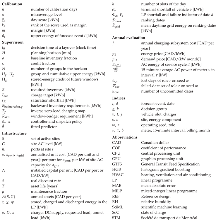
References
- S. S. G. Perumal, R. M. Lusby, J. Larsen, Electric bus planning & scheduling: A review of related problems and methodologies, European Journal of Operational Research 301 (2) (2022) 395–413. [CrossRef]
- Y. He, Z. Liu, Z. Song, Joint optimization of electric bus charging infrastructure, vehicle scheduling, and charging management, Transportation Research Part D: Transport and Environment 117 (2023) 103653. [CrossRef]
- A. Kunith, R. Mendelevitch, D. Goehlich, Electrification of a city bus network: An optimization model for cost-effective placing of charging infrastructure and battery sizing of fast-charging electric bus systems, International Journal of Sustainable Transportation 11 (10) (2017) 707–720. [CrossRef]
- A. P. Zhao, S. Li, Z. Li, Z. Wang, X. Fei, Z. Hu, et al., Electric vehicle charging planning: A complex systems perspective, IEEE Transactions on Smart Grid 16 (1) (2025) 754–772. [CrossRef]
- J. Gu, Q. Liao, K. M. Zhang, Assessing the cold weather impact on battery electric transit buses, Transportation Research Part D: Transport and Environment 145 (2025) 104809. [CrossRef]
- N. A. El-Taweel, A. Zidan, H. E. Z. Farag, Novel electric bus energy consumption model based on probabilistic synthetic speed profile integrated with HVAC, IEEE Transactions on Intelligent Transportation Systems 22 (3) (2021) 1517–1531. [CrossRef]
- M. A. Rahman, D. Holt, Y. Farajpour, A. Mammeri, H. Khiabani, Predictive modeling of energy demands for battery electric buses using real-world data, Energy Informatics 8 (2025) 118. [CrossRef]
- A. Tomaszewska, Z. Chu, X. Feng, S. O’Kane, X. Liu, J. Chen, et al., Lithium-ion battery fast charging: A review, eTransportation 1 (2019) 100011. [CrossRef]
- X. Tian, M. Zhai, S. Wan, H. Peng, Z. Chen, B. Wang, C. An, Assessment of energy efficiency of battery electric buses in cold regions, Transportation Research Part D: Transport and Environment 147 (2025) 104934. [CrossRef]
- J. Dindar, H. Assimi, H. Ranjbar, Sustainable planning of electric bus systems: Degradation-aware and climate-specific techno-economic analysis, Applied Energy 402 (2026) 127039. [CrossRef]
- M. Gallet, T. Massier, T. Hamacher, Estimation of the energy demand of electric buses based on real-world data for large-scale public transport networks, Applied Energy 230 (2018) 344–356. [CrossRef]
- O. A. Hjelkrem, K. Y. Lervåg, S. Babri, C. Lu, C.-J. Södersten, A battery electric bus energy consumption model for strategic purposes: Validation of a proposed model structure with data from bus fleets in China and Norway, Transportation Research Part D: Transport and Environment 94 (2021) 102804. [CrossRef]
- X. Li, T. Wang, J. Li, Y. Tian, J. Tian, Energy consumption estimation for electric buses based on a physical and data-driven fusion model, Energies 15 (11) (2022) 4160. [CrossRef]
- G. E. Karniadakis, I. G. Kevrekidis, L. Lu, P. Perdikaris, S. Wang, L. Yang, Physics-informed machine learning, Nature Reviews Physics 3 (6) (2021) 422–440. [CrossRef]
- J. Willard, X. Jia, S. Xu, M. Steinbach, V. Kumar, Integrating scientific knowledge with machine learning for engineering and environmental systems, ACM Computing Surveys 55 (4) (2023) 66:1–66:37. [CrossRef]
- R. A. Lashaki, Z. Salam, S. Zenhari, M. Mirzamohammadi, Explainable and uncertainty-aware energy prediction for electric bus fleets under heterogeneous operating conditions, Scientific Reports, advance online publication (2026). [CrossRef]
- S. J. Pan, Q. Yang, A survey on transfer learning, IEEE Transactions on Knowledge and Data Engineering 22 (10) (2010) 1345–1359. [CrossRef]
- H. Huang, H. He, Y. Wang, Z. Zhang, T. Wang, Energy consumption prediction of electric vehicles for data-scarce scenarios using pre-trained model, Transportation Research Part D: Transport and Environment 146 (2025) 104830. [CrossRef]
- K. Othman, D. Da Silva, A. Shalaby, B. Abdulhai, Interpretable machine learning models for predicting Ebus battery consumption rates in cold climates with and without diesel auxiliary heating, Green Energy and Intelligent Transportation 4 (2) (2025) 100250. [CrossRef]
- A. N. Elmachtoub, P. Grigas, Smart “Predict, then Optimize”, Management Science 68 (1) (2022) 9–26. [CrossRef]
- L. Sang, Y. Xu, H. Long, Q. Hu, H. Sun, Electricity price prediction for energy storage system arbitrage: A decision-focused approach, IEEE Transactions on Smart Grid 13 (4) (2022) 2822–2832. [CrossRef]
- H. Sheng, Y. Xu, D. Xie, Risk-aware prediction-optimization integrated method for day-ahead microgrid operation, IEEE Transactions on Smart Grid 17 (3) (2026) 2626–2628. [CrossRef]
- D. Fernández-Zapico, T. Hofman, M. Salazar, Stochastic model predictive control of charging energy hubs with conformal prediction, in: 2025 IEEE 64th Conference on Decision and Control (CDC), 2025, pp. 3095–3100. [CrossRef]
- C. Boodoo, Operationalising a digital twin for electric bus dispatch: Quantile-transfer calibration and policy-ready rulebooks, Digital Twins and Applications 3 (1) (2026) e70035. [CrossRef]
- V. Vovk, A. Gammerman, G. Shafer, Algorithmic Learning in a Random World, Springer, New York, 2005. [CrossRef]
- J. Lei, M. G’Sell, A. Rinaldo, R. J. Tibshirani, L. Wasserman, Distribution-free predictive inference for regression, Journal of the American Statistical Association 113 (523) (2018) 1094–1111. [CrossRef]
- A. N. Angelopoulos, S. Bates, Conformal prediction: A gentle introduction, Foundations and Trends in Machine Learning 16 (4) (2023) 494–591. [CrossRef]
- Y. He, Z. Liu, Z. Song, Integrated charging infrastructure planning and charging scheduling for battery electric bus systems, Transportation Research Part D: Transport and Environment 111 (2022) 103437. [CrossRef]
- S. Momen, Y. Maknoon, B. van Arem, S. S. Azadeh, Designing a robust and cost-efficient electrified bus network with sparse energy consumption data, Transportation Research Part C: Emerging Technologies 171 (2025) 105020. [CrossRef]
- L. Ricard, G. Desaulniers, A. Lodi, L.-M. Rousseau, Chance-constrained battery management for electric bus scheduling, European Journal of Operational Research, in press (2026). [CrossRef]
- Z. Yan, T. Zhao, Y. Xu, L. H. Koh, J. Go, W. L. Liaw, Data-driven robust planning of electric vehicle charging infrastructure for urban residential car parks, IET Generation, Transmission & Distribution 14 (26) (2020) 6545–6554. [CrossRef]
- D. Jefferies, D. Göhlich, A comprehensive TCO evaluation method for electric bus systems based on discrete-event simulation including bus scheduling and charging infrastructure optimisation, World Electric Vehicle Journal 11 (3) (2020) 56. [CrossRef]
- J. A. Manzolli, A. V. D’Apice, P. K. Pandey, F. Ciari, L. Miranda-Moreno, Planning resilient electric bus operations in cold regions: An agent-based simulation-optimization framework, Applied Energy 413 (2026) 127735. [CrossRef]
- E. Balogun, E. Buechler, S. Bhela, S. Onori, R. Rajagopal, EV-EcoSim: A grid-aware co-simulation platform for the design and optimization of electric vehicle charging infrastructure, IEEE Transactions on Smart Grid 15 (3) (2024) 3114–3125. [CrossRef]
- H. Hu, B. Du, W. Liu, P. Perez, A joint optimisation model for charger locating and electric bus charging scheduling considering opportunity fast charging and uncertainties, Transportation Research Part C: Emerging Technologies 141 (2022) 103732. [CrossRef]
- Y. Zhou, H. Wang, Y. Wang, R. Li, Robust optimization for integrated planning of electric-bus charger deployment and charging scheduling, Transportation Research Part D: Transport and Environment 110 (2022) 103410. [CrossRef]
- Y. Zhou, G. P. Ong, Q. Meng, H. Cui, Electric bus charging facility planning with uncertainties: Model formulation and algorithm design, Transportation Research Part C: Emerging Technologies 150 (2023) 104108. [CrossRef]
- K. Liu, H. Gao, Y. Wang, T. Feng, C. Li, Robust charging strategies for electric bus fleets under energy consumption uncertainty, Transportation Research Part D: Transport and Environment 104 (2022) 103215. [CrossRef]
- J. A. Manzolli, J. P. F. Trovão, C. Henggeler Antunes, Electric bus fleet charging management: A robust optimisation framework addressing battery ageing, time-of-use tariffs, and energy consumption uncertainty, Applied Energy 381 (2025) 125137. [CrossRef]
- J. N. Hendriks, B. C. P. Sturmberg, An integrated model of electric bus energy consumption and optimised depot charging, npj Sustainable Mobility and Transport 1 (1) (2024) 10. [CrossRef]
- B. Verbrugge, T. Geury, O. Hegazy, Co-design optimization and total cost of ownership analysis of an electric bus depot microgrid with photovoltaics and energy storage systems, Energies 17 (24) (2024) 6233. [CrossRef]
- J. Whitaker, D. Redmond, G. Droge, J. Gunther, Scheduling battery-electric bus charging under stochasticity using a receding-horizon approach, IEEE Transactions on Intelligent Transportation Systems 26 (11) (2025) 19907–19920. [CrossRef]
- R. Lacombe, N. Murgovski, S. Gros, B. Kulcsár, Integrated charging scheduling and operational control for an electric bus network, Transportation Research Part E: Logistics and Transportation Review 186 (2024) 103549. [CrossRef]
- H. Chen, J. Tang, B. Lou, L. Hu, Electric vehicles energy consumption prediction based on seasonal transfer learning model, IEEE Transactions on Transportation Electrification 12 (3) (2026) 4408–4421. [CrossRef]
- NASA Langley Research Center, Prediction of worldwide energy resources (POWER) project: Hourly API, version 2.10.2, accessed 22 September 2026 (2026). URL https://power.larc.nasa.gov/docs/services/api/temporal/hourly/.
- R. Gelaro, W. McCarty, M. J. Suárez, R. Todling, A. Molod, L. Takacs, et al., The Modern-Era Retrospective Analysis for Research and Applications, version 2 (MERRA-2), Journal of Climate 30 (14) (2017) 5419–5454. [CrossRef]
- A. L. Buck, New equations for computing vapor pressure and enhancement factor, Journal of Applied Meteorology 20 (12) (1981) 1527–1532. [CrossRef]
- Buck Research Instruments, LLC, Model CR-2 Hygrometer: Operating Manual, Buck Research Instruments, LLC, Boulder, Colorado, appendix 1: Humidity Conversion Equations, revised July 1996, pp. 19–20 (December 2009). URL https://www.hygrometers.com/wp-content/uploads/CR-2-users-manual-2009-12.pdf.
- D. B. Crawley, L. K. Lawrie, F. C. Winkelmann, W. F. Buhl, Y. J. Huang, C. O. Pedersen, et al., EnergyPlus: Creating a new-generation building energy simulation program, Energy and Buildings 33 (4) (2001) 319–331. [CrossRef]
- P. Fritzson, A. Pop, K. Abdelhak, A. Asghar, B. Bachmann, W. Braun, et al., The OpenModelica integrated environment for modeling, simulation, and model-based development, Modeling, Identification and Control 41 (4) (2020) 241–285. [CrossRef]
- F. Widmer, A. Ritter, C. H. Onder, ZTBus: A large dataset of time-resolved city bus driving missions, Scientific Data 10 (2023) 687. [CrossRef]
- D. P. Kingma, J. L. Ba, Adam: A method for stochastic optimization, in: 3rd International Conference on Learning Representations (ICLR), San Diego, 2015.
- J. H. Friedman, Greedy function approximation: A gradient boosting machine, The Annals of Statistics 29 (5) (2001) 1189–1232. [CrossRef]
- F. Pedregosa, G. Varoquaux, A. Gramfort, V. Michel, B. Thirion, O. Grisel, et al., Scikit-learn: Machine learning in Python, Journal of Machine Learning Research 12 (2011) 2825–2830. URL https://jmlr.org/papers/v12/pedregosa11a.html.
- Q. Huangfu, J. A. J. Hall, Parallelizing the dual revised simplex method, Mathematical Programming Computation 10 (1) (2018) 119–142. [CrossRef]
- B. Efron, Bootstrap methods: Another look at the jackknife, The Annals of Statistics 7 (1) (1979) 1–26. [CrossRef]
- H. R. Künsch, The jackknife and the bootstrap for general stationary observations, The Annals of Statistics 17 (3) (1989) 1217–1241. [CrossRef]
- D. N. Politis, J. P. Romano, The stationary bootstrap, Journal of the American Statistical Association 89 (428) (1994) 1303–1313. [CrossRef]
- S. Holm, A simple sequentially rejective multiple test procedure, Scandinavian Journal of Statistics 6 (2) (1979) 65–70. URL https://www.jstor.org/stable/4615733.
- Y. Benjamini, Y. Hochberg, Controlling the false discovery rate: A practical and powerful approach to multiple testing, Journal of the Royal Statistical Society: Series B (Methodological) 57 (1) (1995) 289–300. [CrossRef]
- R. F. Barber, E. J. Candès, A. Ramdas, R. J. Tibshirani, Conformal prediction beyond exchangeability, The Annals of Statistics 51 (2) (2023) 816–845. [CrossRef]
- Y. Xia, Y. Xu, Learning-based optimal power bidding of an overseas photovoltaic-battery storage plant in Singapore electricity market, Applied Energy 407 (2026) 127328. [CrossRef]
- X. Jia, Y. Xia, Z. Yan, H. Gao, D. Qiu, J. M. Guerrero, Z. Li, Coordinated operation of multi-energy microgrids considering green hydrogen and congestion management via a safe policy learning approach, Applied Energy 401 (2025) 126611. [CrossRef]
Figure 1.
Monthly requested fleet energy at the Reference design in 2025, averaged over 30 operating seeds: (a) Montréal and (b) Singapore. Numbers above bars give non-traction shares (%). Upper curves show mean daily demand on identical right-hand scales (MWh/day): 1.73 to 2.44 in Montréal and 2.61 to 2.71 in Singapore. Montréal heating accounts for 30% to 32% from December to February; Singapore cooling and dehumidification account for 34% to 36% throughout the year. Fans, battery thermal management and other loads together contribute 8.3% to 10.2% and 5.3% to 5.6%, respectively.
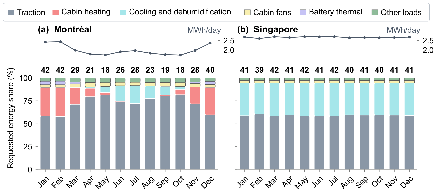
Figure 2.
Directional transfer accuracy. (a, b) Event MAE versus target fitting days for Singapore-to-Montréal; (c, d) Montréal-to-Singapore. Panels (a, c) show 2024 with open markers and (b, d) show 2025 with filled markers. Learning values average 15 seed-subset cells, including five distinct gradient-boosting fits. The calibrated physical prior is independent of target fitting days and appears as horizontal lines in (a, b). In (c, d), it lies above the axis range: MAE is 4.81 kWh in 2024 and 4.39 kWh in 2025. (e, f) Relative MAE differences at 28 fitting days for Singapore-to-Montréal and Montréal-to-Singapore, respectively, against seven comparators. Differences are 100 × (transfer MAE − comparator MAE) / comparator MAE; intervals are 95% seven-day calendar-block bootstraps. Open and filled circles retain the year encoding; negative values favour transfer. The ns labels indicate Holm-adjusted p ≥ 0.05 within 32 comparisons per direction and year. In reverse transfer in 2025, transfer MAE is 11.3% higher than gradient boosting (95% interval 3.37% to 17.87%). Transfer uses anchoring for Singapore-to-Montréal and source coordinates for Montréal-to-Singapore.
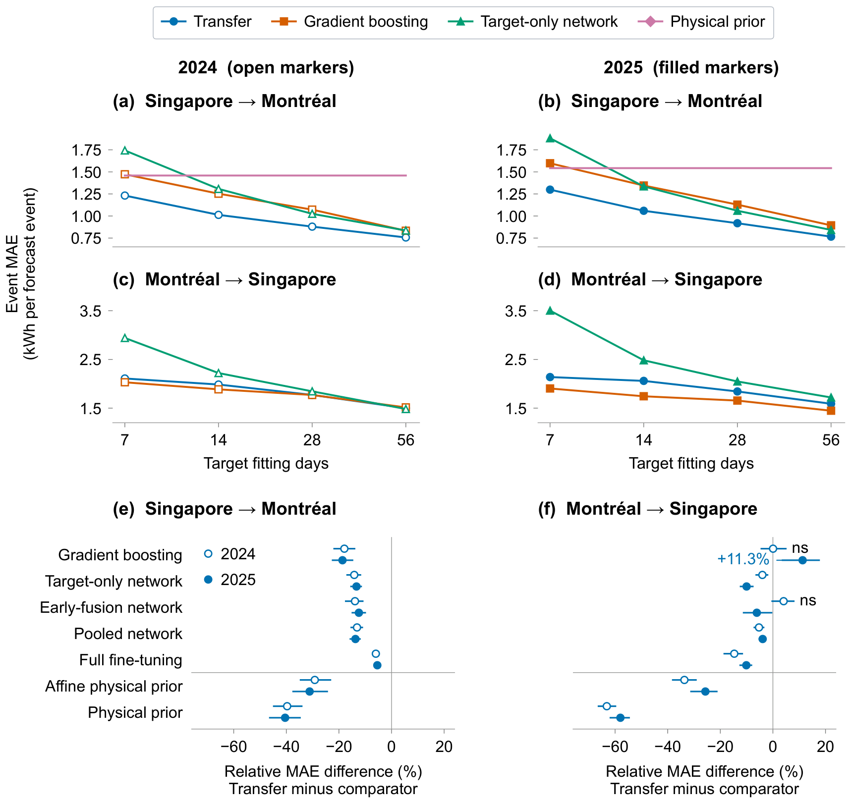
Figure 3.
Forecast characteristics and reserve outcomes, Singapore Registered design. (a) Calibration margin, event MAE and fixed-control annual lost days for five predictors ordered by margin: source-only (SRC), gradient boosting (HGB), target-only network (TGT), source-coordinate transfer (TRF) and calibrated physical prior (PHY). Both years use the same fits. Spearman loss correlations with margin and MAE: −1.00 and 0.10 each year (descriptive, n = 5). (b) 2024 annual lost days: fixed control (controller 5, remaining-window dispatch) versus predictor-specific pairing (controller 6, window-budget dispatch). TRF pairing includes anchoring; PHY retains fixed control. (c) Monthly Reference-relative lost days, including uncommitted dates; (d) absolute failed-cycle share, including Reference (REF) failures. Matrix blocks: 2024 (left, N = 10), 2025 (right, N = 30); columns: operating seeds. SRC strands on every seed before year-end; uncommitted dates count as lost. Reference’s zero relative loss excludes it from (c); SRC’s incomplete years exclude it from (d). Seeds sample passenger and traction randomness around one frozen fit per predictor. Matrices are descriptive; inference uses annual paired contrasts and block bootstraps.
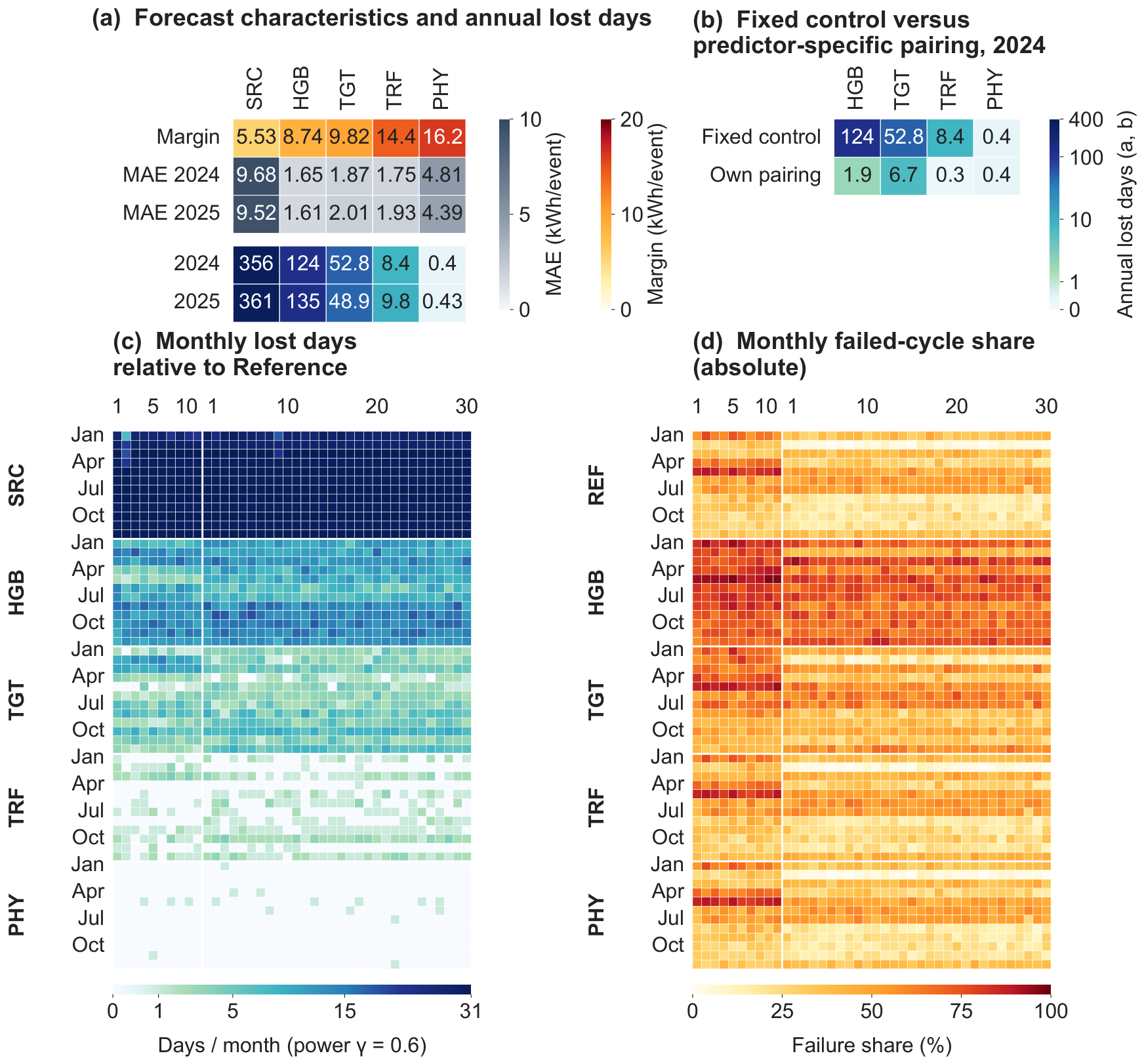
Figure 4.
Resource sensitivities and closed-loop stress outcomes. (a) Cheapest LP-feasible design versus net battery acceptance. Lines connect registered acceptance values as reading guides. AC rating per site is 300 kW at 175 and 245 kW, 450 kW at 350 kW, and 450 kW in Montréal or 600 kW in Singapore at 525 kW. Singapore has no LP-ranked day at 175 kW: all 27 dates are certified infeasible. (b) LP-ranked, certified-infeasible and unserved shares of reference dates (Montréal: 26; Singapore: 27). Base denotes the 245 kW baseline; COP multiplies heating and cooling coefficients of performance (1.2 or 0.8); Load multiplies passenger sensible and latent loads and door exchange (1.5); RH denotes the humidity target (70% or 55%). At 55%, Singapore has no fully served reference date; the comfort ceiling remains 65% RH. (c) Feasible cycles across 11 stress conditions at Registered designs (44 cycles per network and predictor). (d) Weather-crossing feasibility: a run stops at its first stranded vehicle; labels give feasible over executed cycles. Singapore’s network under Montréal weather executes three cycles per arm (20/30 feasible). Stress and crossing use operating seed 1000.
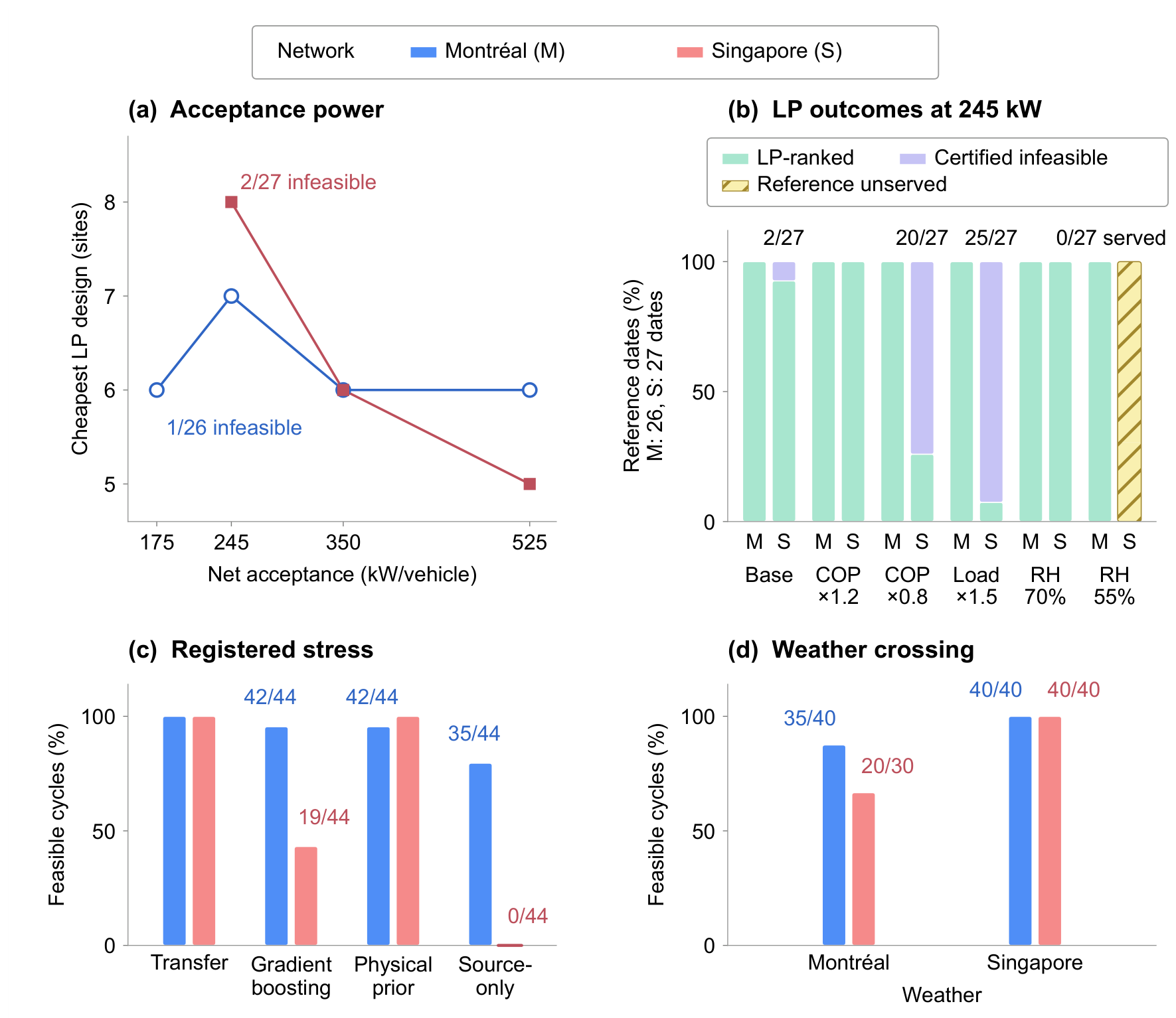
Figure 5.
Reliability and charging-subsystem cost, 2025 (30 operating seeds). (a) Same-seed Reference-relative lost days (symlog): additional failures and uncommitted dates. Dots: seeds; white circles: means; horizontal ticks: medians; vertical lines: Q1–Q3. Eligible seeds and mean lost days of all ten roles: Table S36 (supplement). First five: Registered hardware, controller 5, remaining-window dispatch. Source-only, Adapted transfer: all sites, controller 7, window-budget dispatch. Last three: eight-site designs and Reference. Joint pairing: anchored transfer, controller 6, window-budget dispatch. Singapore Adapted and Registered transfer: source coordinates. (b, c) Costs average complete annual records. Ref., Reg., Qual., F-free, LP-min.: Reference, Registered, qualified predictive, forecast-free, LP minimum. Montréal qualified eight-site savings: 28.2% versus Reference, 17.6% versus Registered (30 paired seeds, both designs relatively eligible). The forecast-free design uses different sites and dispatch; Singapore’s three eight-site costs differ by under 0.2%. Singapore Joint pairing: 9.7% lower mean cost than Reference (descriptive means). Hatching: Montréal’s seven-site LP minimum fails the coldest development date. Singapore Reference averages 113.9 absolute failed days despite zero relative loss. The Registered source-only network strands on every seed before year-end and has no complete annual cost.
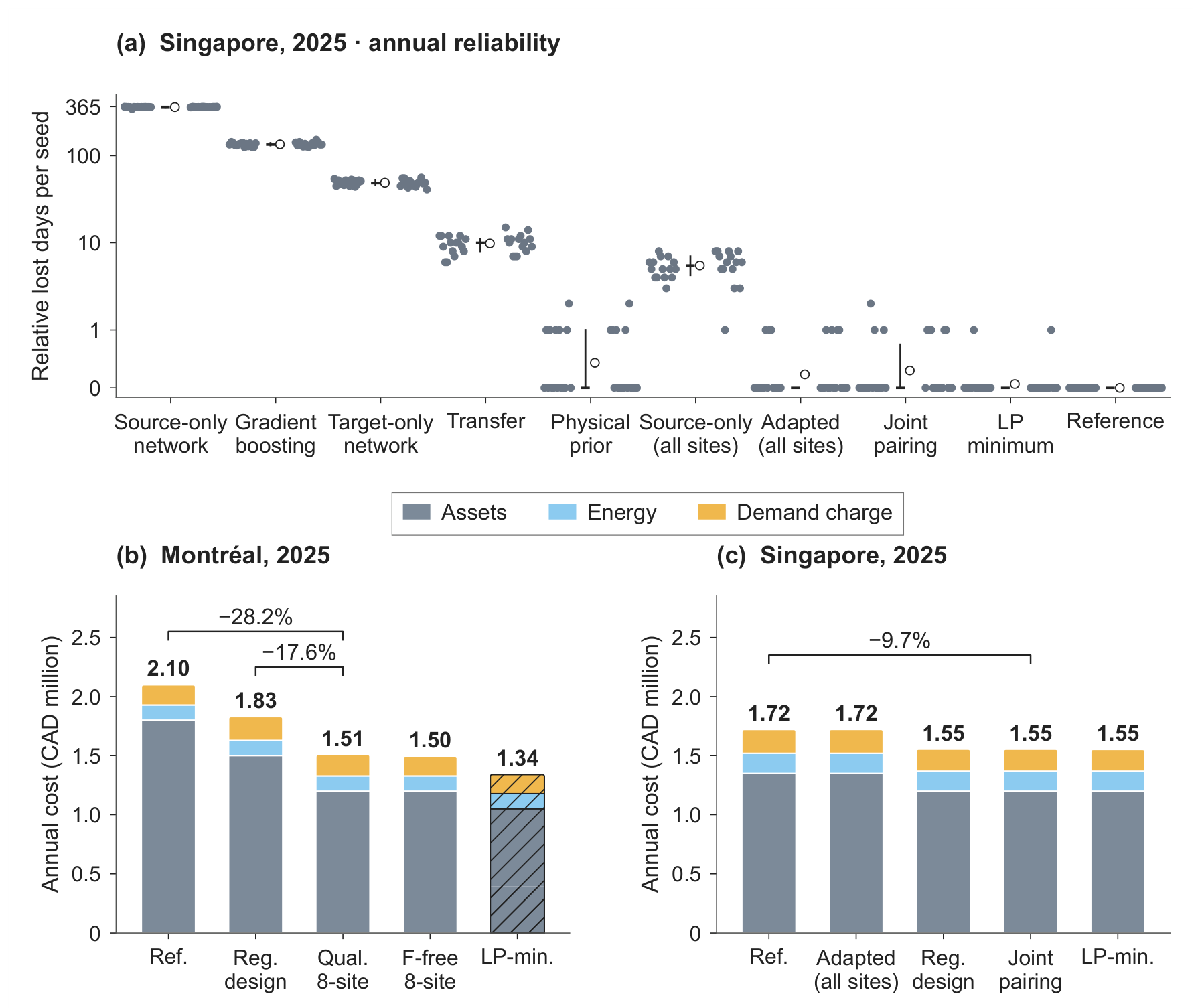

Table 1.
Closest published studies and the capabilities that this study couples. Marks identify capabilities documented in the examined abstracts and methods. Pred., learned energy prediction; Unc., modelled or calibrated energy uncertainty; Transfer, transfer across climates or seasons; Ctrl., supervisory charging control; Infra., charging infrastructure selection; Loop, closed-loop qualification; Cost, annual cost of the charging subsystem.
| Study | Pred. | Unc. | Transfer | Ctrl. | Infra. | Loop | Cost |
| He et al. 2022 [28] | (✓) | ✓ | ✓ | (✓) | ✓ | ||
| He et al. 2023 [2] | (✓) | ✓ | ✓ | ||||
| Hu et al. [35] | (✓) | (✓) | ✓ | ✓ | |||
| Zhou et al. 2022 [36] | ✓ | (✓) | ✓ | (✓) | |||
| Zhou et al. 2023 [37] | (✓) | (✓) | ✓ | (✓) | ✓ | ||
| Liu et al. 2022 [38] | ✓ | (✓) | (✓) | ||||
| Momen et al. [29] | ✓ | ✓ | (✓) | ||||
| Ricard et al. [30] | ✓ | (✓) | (✓) | ||||
| Manzolli et al. 2025 [39] | ✓ | (✓) | (✓) | ||||
| Dindar et al. [10] | n.v. | ✓ | n.v. | ✓ | |||
| Manzolli et al. 2026 [33] | (✓) | (✓) | ✓ | ✓ | |||
| Jefferies and Göhlich [32] | (✓) | (✓) | ✓ | (✓) | ✓ | ||
| Hendriks and Sturmberg [40] | ✓ | ✓ | (✓) | ✓ | |||
| Verbrugge et al. [41] | ✓ | (✓) | (✓) | ✓ | |||
| Whitaker et al. [42] | (✓) | ✓ | (✓) | (✓) | |||
| Lacombe et al. [43] | (✓) | ✓ | (✓) | (✓) | |||
| Fernández-Zapico et al. [23] | ✓ | ✓ | ✓ | (✓) | (✓) | ||
| Boodoo [24] | ✓ | ||||||
| Lashaki et al. [16] | ✓ | ✓ | |||||
| Chen et al. [44] | ✓ | ✓ | |||||
| This study | ✓ | ✓ | ✓ | ✓ | ✓ | ✓ | ✓ |
A mark in parentheses records one element of the capability. The elements are a scenario treatment of uncertain travel time, dwell time, passenger demand or energy use (Unc.), an offline charging schedule or a rule-based charging logic (Ctrl.), depot assets with fixed chargers (Infra.), a closed-loop test of the controller alone or of the design with a rule-based controller (Loop), and charger assets or operation alone (Cost). Ctrl. covers supervisory control of charging or of the storage that serves it. A blank cell indicates a capability not established in the examined sources. For Dindar et al., n.v. identifies control and closed-loop details awaiting full-text verification.
Table 2.
Climate and duties of the two cases. Panel A lists the NASA POWER weather of the development year and the evaluation years, with extremes over daily means of complete local days; the moist-air enthalpy uses the saturation vapour pressure of Buck [47], with coefficients from the July 1996 revision [48] (Section S2 of the supplement) at 101.325 kPa. Panel B lists the six reconstructed duties of each city with the route, the daily distance in km and the daily span in hours (h), both including the off-service return to the depot.
| A. Weather inputs of the development year and the evaluation years | |||||||
| Montréal | Singapore | ||||||
| 2022 | 2024 | 2025 | 2022 | 2024 | 2025 | ||
| Mean temperature [°C] | 6.9 | 8.5 | 7.2 | 27.1 | 27.8 | 27.4 | |
| Mean relative humidity [%] | 79.9 | 80.6 | 77.9 | 85.2 | 86.0 | 86.4 | |
| Mean moist-air enthalpy [kJ/kg] | 22.5 | 25.5 | 22.4 | 76.6 | 80.0 | 78.3 | |
| Lowest daily mean temperature [°C] | -29.9 | -20.2 | -20.2 | 25.0 | 25.6 | 25.0 | |
| Highest daily mean temperature [°C] | 28.1 | 27.1 | 28.7 | 29.2 | 29.7 | 29.3 | |
| B. Reconstructed duties | |||||||
| Montréal | Singapore | ||||||
| Duty | Route | km | h | Route | km | h | |
| 1 | 204 | 311.1 | 18.6 | 169 | 234.5 | 15.3 | |
| 2 | 123 | 180.6 | 18.0 | 61 | 226.2 | 14.3 | |
| 3 | 127 | 237.2 | 18.0 | 67 | 266.8 | 16.4 | |
| 4 | 125 | 148.2 | 18.0 | 854 | 223.0 | 14.6 | |
| 5 | 121 | 204.8 | 17.9 | 966 | 254.0 | 13.3 | |
| 6 | 61 | 233.0 | 18.9 | 985 | 258.5 | 15.5 | |
| Candidate terminals | 12 | 9 | |||||
| Operating events | 9640 | 5592 | |||||
Table 3.
Principal plant and economic parameters with their evidence class. Engineering scenarios are common to both cities.
Table 3.
Principal plant and economic parameters with their evidence class. Engineering scenarios are common to both cities.
| Component | Quantity and value | Evidence class |
| Duties | STM GTFS trips (Montréal) and SimplyGo route guide (Singapore); six duties per city | Official schedule, reconstructed linking |
| Weather | NASA POWER hourly reanalysis, 2019 to 2025; 61368 hourly rows per city | Official reanalysis |
| Battery | 350 kWh; SoC window 0.15 to 0.95; efficiencies 0.98 | Engineering scenario |
| Acceptance | 245 kW plateau; multipliers 1, 0.5 and 0.25 below SoC 0.80, from 0.80 to 0.90 and above 0.90; temperature factor 0 at °C to 1 at 15 °C | Engineering scenario |
| Chargers | 450 kW DC rating; AC-to-DC efficiency 0.92; depot 150 kW per vehicle | Source-anchored engineering scenario |
| Cabin | Heating 32 kW, cooling 35 kW, reheat 20 kW; set points 20 and 24 °C; humidity set point 60%; comfort 18 to 26 °C, relative humidity up to 65% | Engineering scenario |
| Battery thermal | 2 MJ/K; 65 W/K to ambient; control interval 15 to 35 °C | Engineering scenario |
| Capital and life | CAD 1448823.53 per port and CAD 301.84 per kW of grid; lives 15 and 30 years; discount rate 0.04 | Source-anchored engineering scenario |
| Prices | Energy 0.15 CAD/kWh; demand 10 CAD/(kW month) | Engineering scenario |
| Plant reference | Zurich trolleybus missions, ten whole-mission holdouts | Measured, other platform |
Table 4.
Chronology of the study.
| Period | Role | Units | Seeds |
| 2019 to 2021 | Predictor fitting | 1094 Montréal and 1093 Singapore days; budgets of 0, 7, 14, 28 and 56 days | 5 subsets; seeds 101, 202, 303 |
| 2022 | Development | 24 prediction days; 26 Montréal and 27 Singapore co-design dates, with 25 Singapore dates ranked after 2 deficit certificates; transfer variant, screening and selection | |
| 2023 | Calibration | 40 days per city for the margin m | |
| 2024 | First evaluation year | 364 learning dates; 366 annual dates | Operating seeds 1000 to 1009 |
| 2025 | Confirmation year | 363 learning dates; 365 annual dates | Operating seeds 2000 to 2029 |
Montréal weather of 2025 was available during development; Singapore weather of 2025 became available with the confirmation runs. The registered joint choices were selected on the 2022 development dates on 24 September 2026, and their annual populations ran from 24 to 27 September. The complete-domain screening of the 72 Montréal designs, submitted on 27 September at 19:22 and running from 19:28 until stage 2 completed at 20:36 (America/Toronto), used the 2022 development dates only. The two eight-site cases were registered at 20:42 the same day, and their annual execution started on 28 September at 05:33.
Table 5.
Annual comparison roles of the main text. Sites and controllers are listed as Montréal; Singapore. All active sites have 300 kW of AC capacity, and the codes follow the supplementary registry, which lists the remaining roles with the transfer variant of each. The roles listed here use the anchored transfer variant in Montréal. In Singapore, the Adapted and Registered roles use the source-coordinate variant and the Joint pairing uses the anchored variant. Fixed control is the controller and dispatch of the Registered design.
| Role | Predictor | Sites | Controller and dispatch | Code |
| Reference | Forecast-free | 12; 9 | 7, maximum inventory | REF |
| LP-minimum design | Forecast-free | 7; 8 | 7, maximum inventory | LPMIN |
| Source-only | Source-only, 0 days | 12; 9 | 7, window budget | A0 |
| Adapted | Transfer, 28 days | 12; 9 | 7, window budget | A1 |
| Registered design | Transfer, 28 days | 10; 8 | 6; 5, remaining window | A3 |
| Predictor swap | Alternative predictor | 10; 8 | 6; 5, remaining window | SWAP |
| Joint pairing | Predictor-specific | 10; 8 | Predictor-specific | JOINT |
| Qualified eight-site design | Anchored transfer, 28 days | 8; not run | 6, remaining window | A3 lattice |
| Forecast-free eight-site design | Forecast-free | 8; not run | 7, maximum inventory | MAXINV lattice |
Table 6.
Event MAE by target fitting budget and paired difference to gradient boosting (HGB). MAE is in kWh per forecast event, averaged over 15 fits. Differences are transfer minus HGB with 95% intervals from seven-day calendar-block bootstraps, and adjusted p is the Holm value within 32 comparisons per direction and year. Percentages in the text use unrounded MAE.
| Days | Transfer | HGB | Target-only | Difference (95% interval) | Relative [%] | Adjusted p |
| Singapore to Montréal (anchored transfer), 2024 | ||||||
| 7 | 1.232 | 1.473 | 1.743 | −0.241 (−0.294 to −0.190) | −16.4 | ≤ 0.0064 |
| 14 | 1.013 | 1.253 | 1.307 | −0.240 (−0.302 to −0.175) | −19.2 | ≤ 0.0064 |
| 28 | 0.880 | 1.072 | 1.025 | −0.192 (−0.237 to −0.148) | −17.9 | ≤ 0.0064 |
| 56 | 0.757 | 0.833 | 0.836 | −0.076 (−0.108 to −0.044) | −9.1 | ≤ 0.0064 |
| Singapore to Montréal (anchored transfer), 2025 | ||||||
| 7 | 1.299 | 1.598 | 1.881 | −0.299 (−0.354 to −0.243) | −18.7 | ≤ 0.0064 |
| 14 | 1.059 | 1.345 | 1.336 | −0.286 (−0.349 to −0.225) | −21.3 | ≤ 0.0064 |
| 28 | 0.918 | 1.129 | 1.060 | −0.211 (−0.256 to −0.164) | −18.7 | ≤ 0.0064 |
| 56 | 0.766 | 0.894 | 0.842 | −0.128 (−0.166 to −0.088) | −14.3 | ≤ 0.0064 |
| Montréal to Singapore (source-coordinate transfer), 2024 | ||||||
| 7 | 2.109 | 2.032 | 2.941 | 0.078 (−0.001 to 0.157) | 3.8 | 0.31 |
| 14 | 1.985 | 1.886 | 2.221 | 0.099 (0.002 to 0.201) | 5.2 | 0.31 |
| 28 | 1.772 | 1.771 | 1.846 | 0.001 (−0.083 to 0.092) | 0.1 | 1.00 |
| 56 | 1.500 | 1.516 | 1.482 | −0.016 (−0.087 to 0.062) | −1.0 | 1.00 |
| Montréal to Singapore (source-coordinate transfer), 2025 | ||||||
| 7 | 2.139 | 1.904 | 3.503 | 0.235 (0.121 to 0.328) | 12.3 | ≤ 0.0064 |
| 14 | 2.060 | 1.744 | 2.483 | 0.316 (0.161 to 0.447) | 18.1 | ≤ 0.0064 |
| 28 | 1.843 | 1.656 | 2.048 | 0.187 (0.056 to 0.296) | 11.3 | ≤ 0.0064 |
| 56 | 1.591 | 1.448 | 1.720 | 0.143 (0.042 to 0.223) | 9.9 | ≤ 0.0064 |
Table 7.
Frozen predictors at Singapore’s Registered design. Learned deployment fits use model seed 101 and target-day subset 0 at each arm’s budget; the physical prior is deterministic. Fixed control uses controller 5 and remaining-window dispatch. Fixed transfer uses source coordinates, and the joint transfer column uses anchoring, as specified in the table note.
| Predictor | MAE | Bias | Margin | Mean headroom |
Failed cycles [%] |
Lost days (eligible seeds) | |
| kWh per forecast event | Fixed | Joint | |||||
| 2025, 30 operating seeds | |||||||
| HGB | 1.605 | −0.534 | 8.735 | 8.201 | 68.2 | 135.03 (0) | n/a |
| Target-only | 2.013 | −0.285 | 9.821 | 9.536 | 44.6 | 48.90 (0) | n/a |
| Transfer | 1.932 | −0.896 | 14.362 | 13.466 | 33.8 | 9.80 (0) | 0.30 (22) |
| Physical prior | 4.386 | −4.040 | 16.220 | 12.181 | 31.3 | 0.43 (19) | 0.43 (19) |
| Source-only | 9.517 | −9.340 | 5.535 | −3.805 | n/a | 361.43 (0) | n/a |
| Reference | forecast-free | 31.2 | 0.00 (30) | n/a | |||
| 2024, 10 operating seeds | |||||||
| HGB | 1.649 | −0.802 | 8.735 | 7.933 | 78.0 | 123.80 (0) | 1.90 (0) |
| Target-only | 1.873 | −0.590 | 9.821 | 9.231 | 58.5 | 52.80 (0) | 6.70 (0) |
| Transfer | 1.754 | −0.913 | 14.362 | 13.449 | 46.4 | 8.40 (0) | 0.30 (7) |
| Physical prior | 4.810 | −4.576 | 16.220 | 11.644 | 44.2 | 0.40 (6) | 0.40 (6) |
| Source-only | 9.678 | −9.499 | 5.535 | −3.965 | n/a | 356.10 (0) | n/a |
| Reference | forecast-free | 44.1 | 0.00 (10) | n/a | |||
Bias is forecast minus actual, the mean headroom is the mean upper energy minus the actual energy, which equals the bias plus the margin (all in kWh per forecast event), and failed cycles are the share of seed-days with a failed service cycle. Lost days are means per seed with the relatively eligible seeds in brackets. Fixed control is controller 5 with remaining-window dispatch, and joint pairing assigns each predictor its own design, controller and dispatch; the joint transfer row uses the anchored variant (margin 9.973 kWh). The margins of all fits span 8.735 to 12.771 kWh for gradient boosting, which has five distinct fits (one per target subset) and a frozen fit with the smallest margin, and 8.667 to 15.248 kWh for transfer. Differences in the text use unrounded values.
Table 8.
Closed-loop qualification of the 72 LP-feasible 300 kW Montréal designs with controller 7 and forecast-free maximum-inventory dispatch, by active-site count. Minimum SoC is the lowest value over all vehicles on 15 January 2022; the reserve is 0.15. A failing design leaves the screen at its first failed date.
| Sites | Assets [CAD per year] |
LP-feasible designs |
Passing designs |
Minimum SoC, passing designs |
Minimum SoC, failing designs |
| 7 | 1 050 235 | 4 | 0 | none | 0.110 |
| 8 | 1 200 269 | 16 | 4 | 0.314 | 0.110 |
| 9 | 1 350 303 | 25 | 12 | 0.314 to 0.320 | 0.110 |
| 10 | 1 500 336 | 19 | 13 | 0.314 to 0.320 | 0.110 |
| 11 | 1 650 370 | 7 | 6 | 0.314 to 0.320 | 0.110 |
| 12 | 1 800 403 | 1 | 1 | 0.320 | none |
| All | 72 | 36 | 0.314 to 0.320 | 0.110 |
Table 9.
Annual charging-subsystem cost in 2025, mean over complete-record operating seeds. Costs are CAD per year, lost days are means per seed, and eligible counts refer to relatively eligible seeds. Paired cost contrasts use seeds on which both roles are relatively eligible. Text differences use unrounded values. Montréal’s two eight-site designs use different subsets; its LP minimum fails the coldest development date. Singapore uses source coordinates in Adapted and Registered roles and anchoring in Joint pairing.
| Case | Sites | Assets [CAD/yr] |
Energy [CAD/yr] |
Demand [CAD/yr] |
Total [CAD/yr] |
Lost days [per seed] |
Eligible seeds |
| Montréal | |||||||
| Reference | 12 | 1 800 403 | 128 399 | 170 269 | 2 099 071 | 0.00 | 30 |
| Registered design | 10 | 1 500 336 | 128 355 | 200 783 | 1 829 475 | 0.00 | 30 |
| Qualified eight-site design | 8 | 1 200 269 | 128 373 | 179 508 | 1 508 150 | 0.00 | 30 |
| Forecast-free eight-site design | 8 | 1 200 269 | 128 431 | 167 019 | 1 495 719 | 0.00 | 30 |
| LP-minimum design | 7 | 1 050 235 | 128 436 | 161 487 | 1 340 158 | 0.00 | 30 |
| Singapore | |||||||
| Reference | 9 | 1 350 303 | 169 347 | 200 977 | 1 720 627 | 0.00 | 30 |
| Adapted | 9 | 1 350 303 | 169 310 | 201 369 | 1 720 981 | 0.23 | 23 |
| Registered design | 8 | 1 200 269 | 169 250 | 184 118 | 1 553 637 | 9.80 | 0 |
| Joint pairing, transfer | 8 | 1 200 269 | 169 262 | 183 958 | 1 553 489 | 0.30 | 22 |
| LP-minimum design | 8 | 1 200 269 | 169 315 | 181 756 | 1 551 339 | 0.07 | 28 |
Table 10.
Principal quantitative contrasts. Change is proposed minus baseline, and lost days are means per operating seed. Annual costs follow the complete service-cycle account. The minimum-SoC row refers to the controller-7 maximum-inventory qualification screen on 15 January 2022; the qualified eight-site designs under predictive controller 6 reach 0.219 to 0.220 on that date. Changes are computed from unrounded values.
| Quantity | Baseline | Proposed | Change | Relative [%] |
| Montréal MAE [kWh] | Gradient boosting 1.129 |
Transfer 0.918 |
−0.211 | −18.7 |
| Singapore lost days [per seed] | Source-only 5.50 |
Adapted 0.23 |
−5.27 | −95.8 |
| Singapore lost days, fixed control [per seed] | Gradient boosting 135.03 |
Transfer 9.80 |
−125.23 | −92.7 |
| Singapore lost days, pairing [per seed] | Registered design 9.80 |
Joint pairing 0.30 |
−9.50 | −96.9 |
| Montréal annual cost [CAD] | Registered design 1 829 475 |
Qualified eight-site 1 508 150 |
−321 325 | −17.6 |
| Montréal annual cost [CAD] | Reference 2 099 071 |
Qualified eight-site 1 508 150 |
−590 922 | −28.2 |
| Montréal annual cost [CAD] | LP-minimum design 1 340 158 |
Qualified eight-site 1 508 150 |
+167 991 | +12.5 |
| Montréal minimum SoC | LP-minimum design 0.110 |
Qualified eight-site 0.314 |
+0.204 | n/a |
All rows refer to 2025 except the minimum SoC, which refers to 15 January 2022. The minimum SoC is the lowest value of the maximum-inventory screen; the qualified eight-site designs under controller 6 with remaining-window dispatch reach 0.219 to 0.220.
Disclaimer/Publisher’s Note: The statements, opinions and data contained in all publications are solely those of the individual author(s) and contributor(s) and not of MDPI and/or the editor(s). MDPI and/or the editor(s) disclaim responsibility for any injury to people or property resulting from any ideas, methods, instructions or products referred to in the content. |
© 2026 by the authors. Licensee MDPI, Basel, Switzerland. This article is an open access article distributed under the terms and conditions of the Creative Commons Attribution (CC BY) license (http://creativecommons.org/licenses/by/4.0/).
Copyright: This open access article is published under a Creative Commons CC BY 4.0 license, which permit the free download, distribution, and reuse, provided that the author and preprint are cited in any reuse.