

Submitted:
08 October 2026
Posted:
10 October 2026
You are already at the latest version
Abstract
This paper presents two related benchmark studies of artificial intelligence (AI)-enabled wake scheduling for ultra-low-power devices in Frequency Range 3 (FR3, 7–24 GHz) ultra-massive multiple-input multiple-output (UM-MIMO) Internet of Things (IoT) networks, evaluated as Pareto-frontier trade-offs between energy and access performance. Study 1 benchmarks wake scheduling for narrowband IoT (NB-IoT) devices under simulated bursty traffic, comparing a classical fixed-interval policy, a genie-aided policy with perfect intensity knowledge, and a learned traffic-intensity estimator, and characterizes the energy–latency frontier together with tail (95th-percentile) latency. Study 2 addresses beam-sweep-aware wake scheduling, in which an idle-mode UM-MIMO IoT device must also account for directional beam-sweep paging overhead, and evaluates listen-window policies against a learned arrival-time predictor on an energy–reliability frontier. In both studies, learned, time-varying state estimates did not uniformly improve on well-designed fixed-policy baselines. They helped in specific regimes, substantially reducing tail latency relative to the genie-aided reference in Study 1 and uniquely reaching near-perfect paging reliability in Study 2, whereas simple classical policies remained preferable elsewhere. The mechanism behind each gain differed between the two problems, indicating that gains from learned prediction are regime- and context-dependent rather than universal.
Keywords:
NB-IoT
; power saving mode
; wake scheduling
; artificial intelligence
; energy efficiency
; beam sweeping
; paging
; FR3
; ultra-massive MIMO
; 6G
1. Introduction
This paper reports two complementary benchmark studies of artificial intelligence (AI)-enabled wake scheduling for ultra-low-power Frequency Range 3 (FR3) ultra-massive multiple-input multiple-output (UM-MIMO) Internet of Things (IoT) devices. The two studies are combined because they address the same underlying trade-off between energy and responsiveness under two different sources of timing uncertainty: bursty application traffic (Study 1) and directional beam-sweep paging overhead (Study 2).
Narrowband IoT (NB-IoT) achieves decade-scale battery life primarily through two mechanisms standardized by the Third Generation Partnership Project (3GPP) [1]: power saving mode (PSM), a deep-sleep state configured with a single fixed cycle length, and extended discontinuous reception (eDRX), which similarly extends the interval between paging-channel checks using one configured period. Both are static by design: the same wake-up timer applies whether the device's actual traffic is perfectly uniform or highly bursty. In the applications this technology increasingly targets (maritime asset tracking, smart agriculture, and environmental sensing, all named as target use cases for the commercial low-power wide-area chipset platforms on which it runs), real traffic is rarely uniform. A scheduled heartbeat report recurs at a fixed interval, but event-driven messages (a geofence crossing, a threshold-crossing sensor reading, or a storm-triggered alert) arrive in bursts, often with a predictable diurnal or seasonal component superimposed on unpredictable event timing.
These mechanisms are specified in the 3GPP standards. PSM is entered when the active timer T3324 expires and lasts until the periodic tracking-area-update timer T3412 (or its extended variant) elapses [2], whereas eDRX lengthens the interval between paging occasions and introduces a paging time window within which the device monitors paging [3]. NB-IoT was designed for low device cost, extended coverage, and long battery life [4], and both analytical energy models validated against commercial devices [5] and measurements on operational networks [6] show that the configuration of these timers is among the dominant factors in device energy consumption. Choosing these settings correctly will matter even more in 6G: the ITU-R IMT-2030 framework extends massive machine-type communication toward connection densities of up to 10⁸ devices per square kilometer [7], so fixed, one-size-fits-all timer configurations will be applied to ever larger and more heterogeneous device populations.
This raises a testable question: can an AI-driven policy that learns a device's traffic pattern schedule wake-ups more efficiently than a single fixed timer, and if so, in what sense? Study 1 addresses this question by building an open simulation of realistic NB-IoT traffic, training a compact neural network to predict the local message-arrival intensity from causal features alone, and benchmarking the resulting adaptive scheduling policy against a classical fixed-timer baseline and a genie-aided reference policy that uses the true intensity. The simulated traffic is a non-homogeneous Poisson process that combines a deterministic periodic heartbeat with a diurnally modulated, bursty event component and is generated via the classical thinning method. All three policies share the same scheduling rule, so any measured difference reflects the value of better intensity estimation rather than a different control strategy.
Study 1 makes three contributions: (1) an open, physically grounded NB-IoT traffic simulator and multi-device dataset, released with full source code; (2) a benchmark that isolates the value of learned traffic-intensity estimation from the scheduling rule itself, using real measured hardware energy data; and (3) a complete account of the result, which is a trade-off rather than a uniform improvement. The learned policy does not dominate the classical baseline in the practically relevant mean-latency range, but it substantially improves tail-latency behavior relative to the genie-aided reference and becomes clearly preferable to the classical baseline for latency-tolerant applications. All reported results were obtained by executing the described simulation and training code. Where the initial single-operating-point comparison proved misleading (Section 3.2), we report the correction (a full energy–latency Pareto-frontier comparison) and explain why it was necessary, rather than presenting only the more favorable framing.
Study 2 addresses a second, related source of wake-scheduling uncertainty that is specific to FR3 UM-MIMO deployments: directional beam-sweep paging.
Directional beam-sweep paging is the standardized mechanism by which a 5G New Radio (NR) base station reaches an idle-mode device under beamformed transmission. Rather than broadcasting omnidirectionally, the base station sweeps its beam sequentially across a set of angular sectors, forming a synchronization signal block (SSB) burst set of typically 4–8 beams and up to 64 in millimeter-wave (mmWave) deployments; a device must wake and listen during the portion of the sweep pointed at its own known location to receive its paging occasion [8,9,10]. As FR3 (7–24 GHz) UM-MIMO base stations, expected to anchor early 6G deployment in this “golden band” [11,12,13], narrow their beams to serve growing IoT device densities, both the number of beams in a sweep and the precision required to catch a device's own slot are expected to increase [14]. The timing of this wake-and-listen decision is therefore a quantifiable energy-management problem in its own right, distinct from and complementary to the classical fixed-timer PSM scheduling addressed in Study 1.
Real deployments do not sweep on a perfectly fixed schedule: per-beam dwell time is varied adaptively according to the real-time, per-sector traffic load, a practice that can be modeled via an exponential moving average of beam residence time. A device therefore knows, from broadcast system information, only the nominal (average) expected arrival time of its own beam slot, not its exact realized timing, and must budget a listening margin around that nominal estimate to catch the slot reliably without excessive wasted awake time. Study 2 builds an open simulation of this timing process and tests whether a learned predictor that exploits persistent (not purely random) per-beam traffic-load structure, modeled here with persistence ρ = 0.85 (Section 5.1), can improve on simple, interpretable classical margin policies.
Study 2 makes three contributions: (1) an open, physically grounded simulation of beam-sweep timing uncertainty, which confirms from simulated data the theoretical prediction that uncertainty accumulates as the square root of a device's position in the sweep order; (2) a benchmark of classical and learned listen-window policies across the full energy–reliability trade-off space rather than at a single operating point; and (3) an account of where the learned policy helps and where it does not. The learned policy is not Pareto-dominant everywhere but is uniquely valuable in the high-reliability regime, and we explain the mechanism responsible (re-centering on a historically informed rather than nominal arrival estimate) rather than reporting the result without explanation.
2. Related Work
Hardware measurements of NB-IoT PSM and eDRX current consumption on a commercial module (Nordic nRF9151-DK) quantify the energy cost of each fixed-timer configuration: the average current falls from approximately 1.16 mA with no power saving to 278.6 μA with eDRX (40.96 s cycle) and to 25.34 μA with PSM (60-minute cycle, 2-minute active window) [15,16]. These measured values are used in the Study 1 energy model (Section 3.3).
The underlying question of Study 1, whether a traffic-adaptive wake schedule can outperform a fixed duty cycle, is not new: the wireless sensor network (WSN) medium access control (MAC) literature addressed it two decades earlier in a different protocol context. S-MAC, one of the earliest energy-efficient WSN MAC protocols, uses a fixed, synchronized duty cycle and prioritizes energy conservation and self-configuration over per-node latency [17]. T-MAC was proposed to address this fixed-cycle limitation of S-MAC by adaptively ending a node's active period as soon as no further traffic is detected rather than following a rigid schedule, and it reported substantial energy savings under variable, bursty traffic relative to the fixed approach of S-MAC [18]. A subsequent analytical treatment formalized this energy–latency trade-off with a Markov-chain model applicable to both synchronized (e.g., S-MAC) and asynchronous (e.g., X-MAC) duty-cycled protocols; it provides a methodological precedent for the trade-off analysis in Study 1 (Section 3.2), albeit through analytical modeling of a MAC protocol rather than a learned, simulation-benchmarked policy for cellular NB-IoT [19]. In this light, the finding of Study 1 that adaptivity does not uniformly dominate a fixed schedule (Section 4) is consistent with two decades of WSN MAC research, in which no single duty-cycling strategy has been shown to dominate under all traffic conditions and latency requirements. The contribution of Study 1 is to test this question with a learned, rather than hand-designed, adaptive policy in the context of standardized cellular NB-IoT PSM/eDRX and realistic maritime, agricultural, and environmental traffic.
A growing literature applies reinforcement learning to NB-IoT PSM selection: a 2025 study applied soft actor–critic (SAC) reinforcement learning to adaptive PSM control in a simulated NB-IoT environment and reported balanced improvements in power conservation and network performance relative to Proximal Policy Optimization and Deep Q-Network baselines [20]. That work optimizes PSM/eDRX timer selection within a reinforcement-learning framework. Study 1 instead asks a narrower, more directly testable question: given a fixed scheduling-rule structure, does a learned, time-varying intensity estimate outperform a classical fixed estimate, and in which regions of the energy–latency trade-off space? It answers this question with a full Pareto-frontier benchmark rather than a single reported operating point.
Closer to the cellular setting studied here, a substantial body of work models and optimizes the energy of NB-IoT power-saving configurations. Analytical energy models validated against commercial hardware [5] or developed for diverse application traffic with eDRX and PSM [21] show that decade-scale lifetimes depend on careful parameter choice; a semi-Markov analysis of PSM with periodic uplink reporting derives energy and delay jointly [22]; and a dedicated optimization of PSM and eDRX timers explicitly treats their configuration as a trade-off between energy and downlink latency [23], the same trade-off that Study 1 evaluates across its full operating range. Learning-based approaches have also been applied to the closely related problem of discontinuous reception (DRX): an online actor–critic scheme adapts DRX cycles to bursty machine-type traffic and approaches a bound that assumes perfect traffic knowledge [24], a comparison structurally similar to the genie-aided benchmark of Study 1, and ensemble traffic prediction has recently been used to set connected-mode DRX timing [25]. Independently measured PSM sleep currents for a related Nordic cellular IoT module [26] are of the same order as the values used in the Study 1 energy model (Section 3.3).
Direct-to-cell and non-terrestrial-network (NTN) developments motivate the application space of this work. On 21 July 2025, AST SpaceMobile and AT&T made the first Voice over Long-Term Evolution (LTE) call and short-message-service exchange over satellite using AT&T's spectrum and core network with a standard, unmodified cell phone [27]. Commercial cellular IoT chipsets have also begun to integrate satellite connectivity: Altair's ALT1350 LTE-M/NB-IoT system-on-chip, for example, offers NTN communication options in a single chip alongside terrestrial cellular connectivity [28]. This trend extends the remote-deployment use cases targeted by the Study 1 traffic model (maritime, agricultural, and environmental) to locations without terrestrial coverage. The classical statistical technique used to generate the bursty event traffic, namely simulating a non-homogeneous Poisson process by thinning a dominating homogeneous process, is the well-established method of Lewis and Shedler [29] and is not a contribution of this work.
Related reinforcement-learning-based sleep and duty-cycle scheduling work includes compressive-data-gathering sleep schedulers, lightweight Q-learning duty-cycle MAC protocols, restoration-aware deep reinforcement learning (DRL) scheduling for energy-harvesting IoT, and clustering-plus-DRL approaches to extending sensor-network lifetime [30,31,32,33].
The 3GPP beam-sweep-based paging framework allocates paging transmissions across different beams in different time slots, following the same SSB burst-set structure used for initial cell search and synchronization [34]. A dedicated efficient beam-sweeping paging design reduces the number of sweeping beams and required time slots on the basis of estimated user-equipment mobility and beam residence time (via an exponential moving average of per-beam dwell time), reporting that this allows devices to wake with a longer DRX cycle and save more power than naive total beam sweeping [35]. Machine learning (ML) approaches to beam-sweep timing have been applied primarily to the initial-access (cell-search) phase rather than to the idle-mode paging-wake-timing problem addressed in Study 2: a recurrent-neural-network approach predicts beam-sweeping patterns from the user-traffic distribution to accelerate initial access in standalone mmWave 5G NR [36], and a broader computer-vision-aided beamforming framework argues that the current handshake-based beam management strategy is inefficient in terms of latency and energy across multiple mmWave use cases [37].
The problem addressed in Study 2, namely how much listening margin an idle-mode device should budget around its broadcast nominal beam-slot arrival time, lies between these two literatures. It involves the same beam-sweep-timing uncertainty that the efficient beam-sweeping paging work [35] addresses from the network side, but it poses a device-side wake-scheduling question, analogous to the classical-versus-learned comparison for NB-IoT PSM scheduling in Study 1, rather than a network-side sweep-design question. To our knowledge, no reviewed study has benchmarked a learned device-side listen-window policy against a hand-derived, physically motivated classical alternative across the full energy–reliability operating range for this problem.
Complementary beam-management literature includes AI/ML survey treatments of beam selection and tracking, learned beam-update-period optimization that substantially reduces sweeping overhead, 3GPP standardization perspectives on AI/ML beam management, and wake-up-signal-based NB-IoT power-saving receiver implementations [38,39,40,41].
The broader beam-management literature provides the physical context for Study 2. Directional cell discovery with swept synchronization signals takes longer than omnidirectional search [42], exhaustive beam sweeping trades discovery delay against coverage and overhead [43], and 3GPP NR beam management organizes synchronization and reference signals into swept bursts that a device must monitor in the correct beam's time slot [8]. On the device side, NR power saving relies on DRX configured through radio resource control (RRC) signaling [44], and a survey of DRX-based device power saving from LTE through NR toward 6G documents the Release-16 power-saving signal [45]; idle-mode paging, the focus of Study 2, lies explicitly outside the scope of that survey. As arrays grow from massive [46,47] toward the far larger arrays anticipated for the upper mid-band [13], beams narrow and the number of beams to sweep increases, which has been identified as a key beam-management challenge for 5.5G and 6G [14]; multi-beam beamforming is already used in massive MIMO base stations to serve many users simultaneously [48].
Taken together, these literatures leave two gaps. For Study 1, learned and analytical approaches to PSM, eDRX, and DRX configuration are usually evaluated at a single operating point or through a single aggregate metric, so it is rarely clear where on the energy–latency trade-off a learned policy helps, or whether mean and tail latency tell the same story. For Study 2, beam-sweep timing has been studied mainly from the network side, through sweep design and initial access, whereas the complementary device-side question (how widely an idle-mode device should listen around its expected beam slot, and whether learning helps) has not been benchmarked across the full energy–reliability range. The two studies address these gaps in turn.
Study 1: Traffic-Driven Wake Scheduling
3. Traffic Simulation and Scheduling Methodology
3.1. Traffic Model
Each simulated device generates messages over a 7-day observation window from two independent sources. A deterministic periodic heartbeat recurs every 60 minutes, representing scheduled status reporting. An event-driven component follows a non-homogeneous Poisson process with rate λ(t), simulated via the classical thinning method [29], which combines a smooth diurnal component (with amplitude and phase randomized per device, representing, e.g., daylight-driven agricultural sensor activity) with one to three short, randomly timed high-intensity burst windows (0.5–3 hours duration, 5–20 events/hour, representing, e.g., an alarm episode or a geofence-crossing period). Device parameters (base rate, diurnal amplitude and phase, and burst count, timing, duration, and intensity) are randomized independently per device (150 training, 40 validation, and 50 held-out test devices, entirely non-overlapping), providing traffic diversity rather than a single repeated pattern. This two-component structure follows the characterization of machine-type traffic in the 3GPP machine-type-communication traffic models as a mixture of regular reporting and synchronized, event-driven bursts [49], and the time-varying-rate Poisson description is consistent with the Markov-modulated Poisson models used for heterogeneous machine-to-machine traffic [50].
3.2. Adaptive Scheduling Rule and the Need for a Pareto-Frontier Comparison
All three scheduling policies compared in Study 1 (Section 3.4) use the same rule: given an intensity estimate λ̂(t) (events/hour), the interval until the next wake-up is C/λ̂(t), clipped to a floor of 1 minute (bounding the worst-case latency) and a ceiling of 180 minutes (bounding energy during idle periods), for a fixed design constant C. Initial testing at a single, arbitrarily chosen value of C = 15 produced a result that would have been misleading if reported alone: the genie-aided policy (using the true intensity directly) achieved approximately 7% lower energy than the classical fixed-average-intensity baseline but at 3–4× higher mean latency. This occurs because the single fixed intensity estimate of the classical baseline (the device's long-run average, inflated by the rare high-intensity bursts) is systematically higher than the true intensity during most of the (non-burst) operating time. The classical baseline therefore polls more frequently than an intensity-aware policy would consider necessary, saving latency at the cost of energy rather than the reverse. Because C sets a single, arbitrary operating point on each policy's energy–latency trade-off curve, comparing policies at one fixed C conflates the choice of C with the value of better intensity estimation. Section 4 therefore reports a full sweep across six C values (5, 10, 15, 25, 40, 60) for each policy and compares the resulting Pareto frontiers rather than single points.
3.3. Energy and Latency Evaluation
Energy is computed using real measured NB-IoT current-consumption values for a commercial module (Nordic nRF9151-DK, measured by Qoitech) [15,16]: a deep-sleep (PSM) current of 25.34 μA between wake events and an active current of 1160 μA (the measured no-power-saving baseline current) for a representative 1.5 s active window per wake-check-and-transmit event, at a nominal 3.3 V supply. For a given wake schedule and the true message-arrival times, the per-message latency is the time from message readiness to the next scheduled wake at or after that time, and the energy is the sum of the sleep-time and active-time contributions over the full 7-day window. Mean latency, 95th-percentile (P95, tail) latency, and total energy are reported per device and averaged across the test set. This state-based accounting follows NB-IoT energy models that compute consumption from the time spent in each power state and its measured current [5,21]. Tail latency is reported alongside the mean because rare, long delays can dominate the experience of a service even when the average latency is low [51], and the policies are compared as Pareto frontiers because energy and latency are conflicting objectives with no single optimum [52].
Formally, for a device woken n times over an observation window of duration T, the energy is E = V[I_a n t_a + I_s (T − n t_a)], where V = 3.3 V; I_a = 1160 μA and t_a = 1.5 s are the active-state current and duration per wake event; and I_s = 25.34 μA is the sleep current. Each wake event therefore costs about 5.7 mJ, whereas sleeping costs about 84 μW, or about 7.2 J per day. This makes the role of the wake interval explicit: at the 1-minute floor of the scheduling rule, a device wakes 1440 times per day and spends about 8.3 J per day on wake events, more than its entire daily sleep energy, whereas at the 180-minute ceiling it wakes 8 times per day and spends only about 0.05 J. For a message that becomes ready at time τ, the latency is L = w(τ) − τ, where w(τ) is the first scheduled wake time at or after τ; the reported mean and 95th-percentile latencies are computed over all messages generated by a device during the 7-day window.
3.4. Scheduling Policies
Classical: λ̂ is fixed at the device's long-run average intensity (total messages divided by the observation duration) and does not change over time, which is exactly how a real PSM/eDRX timer is configured today: a single value set once and not adapted to subsequent traffic. Genie-aided: λ̂(t) is the true intensity used to generate the traffic (Section 3.1); this perfect-knowledge reference shows the effect of perfect, rather than merely improved, intensity knowledge. Learned (this study): λ̂(t) is the output of a compact multilayer perceptron (two hidden layers of 32 units, rectified linear unit (ReLU) activation, and a softplus output layer to enforce positivity) that takes as input only information causally available at prediction time: message counts in eight 30-minute sub-windows of the preceding 4 hours, a sine/cosine time-of-day encoding, and the time since the most recent message (11 features in total). The model was implemented in PyTorch [53] and trained with the Adam optimizer [54] using a log-space mean-squared-error (MSE) loss, because the intensity spans two orders of magnitude across the dataset (from 0.05 to 26 events/hour) and a plain MSE loss would be dominated by the rare high-intensity examples. It converged to a held-out test log-MSE of 0.049, a 63% reduction relative to a naive constant-prediction baseline (log-MSE 0.132).
The three policies therefore differ only in the intensity estimate supplied to the common rule of Section 3.2, which allows differences in energy and latency to be attributed to estimation quality alone. Energy and latency are computed per device over the full 7-day window and averaged across the 50 held-out test devices, and each policy is evaluated at all six values of C, giving six points per policy on each energy–latency frontier. Training, validation, and test devices are generated with independent random parameters and never overlap, so the learned model is always evaluated on traffic patterns it has not seen. All simulation, training, and evaluation code is provided as supplementary material (see the Data Availability Statement), so every reported figure can be regenerated.
4. Results
All results were obtained by running the code described in Section 3 and evaluating it on the 50-device held-out test set; no result was written before the corresponding code had been executed.
4.1. Energy–Latency Pareto Frontier
Figure 1 shows that the curve of the classical baseline lay below (better than) or close to that of the learned policy for mean latencies up to approximately 20 minutes, and that the classical baseline reached substantially lower latency (down to 1.5 min at C = 5) than either the learned or the genie-aided policy within the tested C range. Beyond a mean latency of approximately 20–22 minutes, the learned policy's curve moved slightly ahead of the classical baseline's. The genie-aided reference did not dominate either alternative across the tested range, a direct consequence of the single-C conflation identified in Section 3.2: at matched C, the genie-aided policy achieved lower energy but higher latency than the classical policy, not a strict improvement.
4.2. Energy Saving at Matched Latency
Figure 2 quantifies this comparison. Across the practically relevant mean-latency range of 5–20 minutes (appropriate for most periodic IoT reporting applications), the learned policy showed a small negative-to-neutral energy saving relative to the classical policy (−1.3% to +0.3%), and the genie-aided policy was more clearly negative (−3.1% to −0.1%); neither adaptive policy provided a clear energy advantage in this range. The learned policy's saving became modestly positive (up to +0.9%) only beyond a mean latency of roughly 22 minutes. Interpolated values below approximately 5 minutes are not reported quantitatively, because the tested C grid does not sample that region densely and linear interpolation there is unreliable (Section 8).
4.3. Tail (95th-Percentile) Latency
Figure 3 shows a materially different picture from the mean-latency comparison (Figure 1). The tail-latency Pareto curve of the learned policy lay consistently to the left of (better than) the genie-aided curve across the entire tested range: at every matched energy level, the P95 latency of the learned policy was substantially lower than that of the genie-aided policy (e.g., at approximately 14.7 mWh, the learned P95 latency was 31.1 min versus 56.2 min for the genie-aided policy). The learned policy's curve also crossed ahead of the classical baseline's for P95 latencies beyond approximately 20 minutes, similar to the mean-latency crossover in Figure 1 but more pronounced. This tail-latency advantage over the genie-aided policy, despite the use of strictly less information (a learned estimate rather than the true intensity), is explained in Section 4.4.
4.4. Mechanism: Prediction Smoothing as an Implicit Safety Margin
Figure 4 shows why the learned policy outperformed the genie-aided reference on tail latency despite using less accurate information: the learned model tracked the diurnal baseline reasonably well but systematically undershot the sharp burst peaks (predicting 3.9–5.4 events/hour against true peaks of 7.4–7.7 events/hour in this example). Because the scheduling rule shortens the wake interval more aggressively as the intensity estimate increases, the genie-aided policy, which uses the true (higher) peak intensity, commits to very short intervals during bursts and, conversely, to very long intervals during the deepest troughs of the true intensity between bursts. The smoothed, regularized predictions of the learned model approach neither extreme as closely; this costs it a small part of the genie-aided policy's energy saving (Figure 1) but avoids the very long worst-case intervals that cause the poor tail latency of the genie-aided policy (Figure 3). Thus, under this reciprocal scheduling rule, imperfect learned prediction acts as an implicit safety margin against the extreme scheduling decisions that perfect information would otherwise select.
Figure 4 also shows that the classical fixed-average estimate (dashed line) lay above the diurnal baseline for most of the observation window, confirming the mechanism proposed in Section 3.2. Because the long-run average is inflated by the brief, high-intensity bursts, the classical policy polls more frequently than the actual (non-burst) local intensity would justify for most of the trace; this is the direct cause of its better mean and tail latency at matched C, at the cost of the additional energy quantified in Figure 1.
Study 2: Beam-Sweep-Aware Wake Scheduling
5. System Model and Methods
5.1. Beam-Sweep Timing Model
A base station sweeps its beam sequentially across N = 8 angular sectors (matching a representative real SSB/paging burst-set size). The true dwell time of each beam in a given cycle equals a nominal value (10 ms, a representative paging-occasion dwell time) plus real-time jitter, which is modeled with two components: a slowly varying, persistent per-beam load level and faster, memoryless per-cycle noise. The load level follows a first-order autoregressive (AR(1)) process [55] and represents traffic-load persistence across consecutive sweep cycles, since a beam sector serving a consistently busier area tends to have longer dwell times over many cycles rather than purely independent per-cycle noise. A device assigned to beam index k receives its paging occasion at the true (realized) arrival time of beam k within that cycle, which depends on the cumulative true dwell times of all k preceding beams in the sweep. This reflects the structure of NR synchronization and paging, in which SSBs are transmitted as a time-ordered sequence of beam-indexed occasions and paging is transmitted in multiple beams within a paging occasion [9,10]. With independent per-beam jitter, the variance of the arrival time of beam k grows linearly with k, so its standard deviation grows as the square root of k; this accumulated-uncertainty law is tested in Section 6.1.
Formally, in sweep cycle c, the true dwell time of beam j is d_j(c) = d_0 + u_j(c) + ε_j(c), where d_0 = 10 ms is the nominal dwell time, u_j(c) = ρ u_j(c−1) + η_j(c) is the persistent per-beam load component with persistence ρ = 0.85, and ε_j(c) is independent per-cycle noise. A device assigned to beam k therefore receives its paging occasion at t_k(c) = Σ_{j<k} d_j(c) after the start of the sweep, whereas the broadcast nominal arrival time is k·d_0. A listen window of width W centered on an estimate t̂_k scores a hit if it overlaps the true dwell interval of the beam; its awake-time cost is the time from the start of the window until detection on a hit, or W on a miss. The classical policies center the window on k·d_0, whereas the learned policy centers it on its predicted arrival time and sets W from its predicted standard deviation (Section 5.3).
5.2. Listen-Window Policies
A device wakes to listen in a window of width W centered on an estimated arrival time and succeeds (a hit) if its window overlaps the true arrival window of its beam slot. On a miss, the device must wait for its next long-cycle wake attempt, which adds a large latency. The awake-time (energy) cost is the time from the start of the listen window until the beam signal is detected on a hit, or the full window width on a miss. Three policies are compared, all evaluated across a common range of reliability targets by scaling a base window width by a common multiplier z (1.0–3.0): (i) fixed margin, which uses the same window width for every device regardless of its beam index; (ii) beam-index-aware, a hand-derived classical policy that scales the window width with the square root of the target beam index, reflecting the accumulated-jitter growth law confirmed in Section 6.1; and (iii) ML-adaptive (Section 5.3), which re-centers its window on a learned, historically informed predicted arrival time and sizes its width from a learned predicted uncertainty, rather than centering on the broadcast nominal time as both classical policies do.
5.3. Learned Arrival-Time Predictor
A compact multilayer perceptron (two hidden layers of 64 units, ReLU activation) is trained to predict the Gaussian mean and log-standard deviation of a device's beam-slot arrival-time offset from nominal. This mean–variance estimation network is the standard approach for heteroscedastic (input-dependent) uncertainty estimation with neural networks [56,57,58]. Its inputs are a causal window of the dwell times of all beams up to and including the target beam over the five most recent sweep cycles, plus the target beam index (41 input features). The model was implemented in PyTorch [53] and trained with the Adam optimizer [54] using a Gaussian negative-log-likelihood loss on 22,000 examples from 400 simulated devices; it was validated on 5,500 held-out examples from 100 non-overlapping devices and converged without overfitting. At inference, the predicted mean re-centers the listen window, and the predicted standard deviation, scaled by the same multiplier z used for the classical policies, sets its width.
Evaluation uses 150 simulated devices over 55 sweep cycles, with the multiplier z swept from 1.0 to 3.0 so that each policy traces a full energy–reliability curve rather than a single operating point; as described above, the training and validation devices of the learned model do not overlap. The simulation and training code is provided as supplementary material (see the Data Availability Statement), so every reported figure can be regenerated.
5.4. Generative AI Disclosure
Literature retrieval, the beam-sweep-timing and listen-window-policy simulation code, model training, figure generation, and manuscript drafting for this article were carried out with the assistance of an AI language model (Claude, Anthropic) under direct human supervision and iterative review. All reported quantitative results were computed by executing the described simulation and training code. The authors are responsible for verifying, and take full responsibility for, the accuracy of all reported figures, model assumptions, and citations.
6. Results
All results were obtained by running the code described in Section 5; no result was written before the corresponding code had been executed.
6.1. Timing Uncertainty Grows with Sweep Position
Figure 5 confirms from simulated data that timing uncertainty accumulates as a device's target beam moves later in the sweep order, closely matching the theoretical square-root scaling expected when independent per-beam dwell-time jitter accumulates across the preceding beams (standard deviation of 1.51 ms at beam index 1, rising to 4.00 ms at beam index 7, versus a theoretical prediction of 1.51 × √7 = 3.99 ms). This has a practical implication independent of any learned model: devices assigned to later positions in a beam sweep face inherently greater uncertainty about the timing of their own paging occasion and, all else being equal, should be expected to require proportionally larger listening margins than devices earlier in the sweep. A real deployment's beam-index assignment policy could account for this structural effect.
6.2. Energy–Reliability Pareto Frontier
Table 1 and Figure 6 show a trade-off rather than a uniform advantage for the learned policy. In the moderate-reliability regime (hit rates up to approximately 97%), the hand-derived beam-index-aware classical policy was Pareto-optimal, requiring lower energy at a matched hit rate than both the fixed-margin and ML-adaptive policies. A well-designed classical heuristic, grounded in the accumulated-jitter law confirmed in Section 6.1, is thus the most efficient choice in this operating range. The fixed-margin policy was dominated by the beam-index-aware policy over most of the tested range and should generally not be used in preference to it; only at z = 3.0 did the fixed-margin policy reach a slightly higher hit rate (98.2% vs. 97.3%), at a longer mean awake time (5.64 ms vs. 4.30 ms).
The learned policy's curve, however, was the only one of the three to reach near-perfect reliability without disproportionate energy cost: at the highest tested margin multiplier (z = 3.0), it achieved a 99.8% hit rate at a mean awake time of 6.19 ms, whereas the beam-index-aware and fixed-margin policies plateaued at 97.3% and 98.2%, respectively, at the same multiplier, with neither approaching the reliability of the learned policy within the tested range. Reaching comparably high reliability with either classical policy would require extrapolation to substantially larger multipliers than those tested here, at a disproportionate (super-linear, based on the curvature visible in Figure 6) energy cost.
6.3. Mechanism: Re-Centering on Predicted Rather Than Nominal Arrival Time
The advantage of the learned policy in the high-reliability regime has a specific, verifiable mechanism rather than being a mere correlation with model sophistication. Both classical policies center their listen window on the broadcast nominal arrival time and can adjust only the window width, not its position, to trade energy against reliability. Widening a poorly centered window is a comparatively inefficient way to increase the hit probability, because much of the added width covers time ranges in which, given the modeled persistent per-beam load structure (Section 5.1; persistence ρ = 0.85), the true arrival is less likely to fall. The learned policy instead exploits recent per-beam dwell-time history to shift its window toward where, given that history, the true arrival is expected to fall, and then sizes a comparatively narrower window around this better-centered estimate. This re-centering, rather than margin tuning alone, is the source of its efficiency advantage in the high-reliability regime; neither classical policy has this capability by construction, since neither uses per-cycle historical information.
7. Joint Discussion
The central finding of Study 1 is a trade-off rather than a uniform improvement, and this qualification is itself its main contribution. Much of the literature on AI-driven PSM control (Section 2) reports overall improvement metrics without decomposing performance across the full energy–latency operating range, which the results in Section 4 suggest may obscure important structure. A reader evaluating whether to adopt a learned, adaptive wake-scheduling policy for a specific NB-IoT deployment needs to know not only whether it helps on average but also for which target latency and which latency statistic (mean or tail) it helps, because these can point in different directions simultaneously. The same learned policy that failed to beat the classical baseline on mean-latency-matched energy in the 5–20 minute range substantially outperformed the genie-aided reference on tail latency across the entire tested range.
The tail-latency finding (Section 4.3 and Section 4.4) has an actionable implication for real deployments. Applications in which occasional very late message delivery is costly (e.g., a delayed alarm in environmental-hazard monitoring) should treat tail latency, rather than mean latency, as the primary evaluation metric; in that case, the advantage of the learned policy over both alternatives is clearer and appears earlier (at lower target latency) than the mean-latency results alone would suggest. Conversely, applications with strict low-latency requirements throughout (e.g., near-real-time command and control) are better served by the classical fixed-timer approach at low C, at least under the reciprocal scheduling rule tested here; whether a different rule structure (Section 8) could close this gap is an open question for future work rather than a limitation of adaptive scheduling in general.
The mechanism identified in Section 4.4, whereby the smoothing of the learned model's predictions acts as an implicit safety margin against the extreme scheduling decisions that perfect information would select, suggests a testable design implication: an explicitly regularized or uncertainty-aware intensity estimator (even a classical one, e.g., a shrinkage estimator blending the local and long-run averages) might reproduce some of this benefit without requiring a trained model at all. By isolating the estimator from the scheduling rule (Section 3.2), the Study 1 benchmark provides the evaluation framework to test this hypothesis, which we identify as a priority for follow-up work.
The Study 2 discussion below addresses the beam-sweep-specific wake-scheduling trade-off. Taken together, the two studies indicate that a learned, time-varying estimate of scheduling-relevant state improves the achievable trade-off over fixed-policy baselines only in specific regimes (tail latency in Study 1 and near-perfect reliability in Study 2), and that the size and character of this improvement depend on which source of timing uncertainty, traffic burstiness or beam-sweep geometry, dominates in a given deployment.
The practical recommendation of Study 2 is regime-dependent rather than universal. For moderate-reliability applications, in which occasional missed paging occasions, recovered by a retry at the next long-cycle wake attempt, are acceptable, the hand-derived beam-index-aware classical policy is both simpler to implement and more energy-efficient than a learned alternative and should be preferred. For applications requiring near-perfect paging reliability, the learned policy is the only tested option that reaches this regime without disproportionate energy cost, because it is the only policy that exploits the persistent per-beam traffic-load structure modeled here (ρ = 0.85) rather than treating each sweep cycle as independent; the simulation thus shows that learning helps when such persistence is present. Such applications are increasingly relevant as FR3 UM-MIMO networks scale to serve dense IoT deployments, in which missed paging occasions compound into network-wide retry congestion.
This finding is consistent with, and extends, a pattern observed in the authors' companion studies: AI-driven approaches to wireless scheduling and resource allocation do not uniformly dominate well-designed, physically motivated classical heuristics, but they tend to deliver their clearest, most defensible advantage in tail or high-reliability operating regimes, where the inability of classical approaches to exploit historical or structural information becomes most costly. Study 2 adds a mechanistic explanation specific to this problem (window re-centering versus window widening) to that broader pattern and explicitly identifies the underlying enabler (persistent, not purely random, per-beam traffic-load structure), rather than treating the learned policy's advantage as an unexplained black-box outcome.
These results have practical implications beyond the simulated settings. For operators and device makers configuring NB-IoT fleets, Study 1 indicates that learned intensity estimation is worth deploying mainly where latency tolerance is high or tail latency matters, such as environmental alarms or asset tracking with occasional urgent events, whereas a well-chosen fixed timer remains adequate for strict low-latency applications. Because the decision rule is shared, a learned estimator can replace the fixed intensity implicitly assumed when PSM and eDRX timers are configured today without changing the standardized mechanisms themselves [2,3]. For FR3 base-station and chipset designers, Study 2 indicates that listen windows should at least scale with beam position, which requires only the beam index already known to the device, and that learned re-centering is worth its added complexity where near-perfect paging reliability is needed, for example, in dense deployments where missed pages trigger retries. Both findings are relevant to satellite-enabled IoT, where direct-to-device links [27,28] and integrated 5G–satellite IoT architectures [59] extend battery-powered devices to remote locations in which replacing batteries is costly and energy efficiency is correspondingly valuable.
8. Limitations and Future Research Directions
Study 1 has several limitations. First, the traffic model (Section 3.1) is a representative, physically motivated but synthetic non-homogeneous Poisson process; it is not fitted to or validated against real maritime, agricultural, or environmental NB-IoT deployment data, which were not available for this study. Second, the single reciprocal scheduling rule (interval = C/λ̂, Section 3.2) is a simple and interpretable, but not necessarily optimal, control law. A more sophisticated policy (e.g., one incorporating explicit uncertainty quantification, or one separating the known deterministic heartbeat component from the learned bursty-event component rather than treating both as a single intensity) might shift the results reported in Section 4; testing this is left for future work. Third, the interpolated matched-latency comparison (Figure 2) is unreliable below a mean latency of approximately 5 minutes because the tested C grid (5, 10, 15, 25, 40, 60) does not sample that region densely; a finer low-C grid would be needed to characterize the low-latency regime with the same confidence as the rest of the range. Fourth, energy accounting uses real measured current values for one commercial module under one PSM configuration. Different hardware or configurations would shift the absolute energy figures, although the qualitative Pareto-frontier comparison between policies is a property of the traffic model and scheduling rule rather than of the particular current values used. Fifth, this is a single-realization benchmark (one trained model and one 50-device test set); repeating training with multiple random seeds would strengthen confidence in the reported gains. Sixth, Study 1 does not report field measurements or a hardware implementation; it is a simulation-based benchmark, and the absolute energy and latency figures should be interpreted as illustrating a methodological finding (the mean/tail-latency distinction and its cause) rather than as validated operational targets for a specific deployed system.
Study 2 also has limitations. First, the persistent traffic-load model (Section 5.1; AR(1) process with persistence 0.85) is a representative, physically motivated but synthetic model; it is not fitted to or validated against real beam-sweep dwell-time measurements from an operational FR3 or mmWave deployment, which were not available for this study. Second, the comparison uses a single representative sweep configuration (8 beams, 10 ms nominal dwell time). Other beam-count or dwell-time configurations, particularly the much larger beam counts (up to 64) possible in mmWave deployments, were not evaluated and could shift the specific quantitative results, although the qualitative mechanism (accumulated timing uncertainty growing with sweep position, and learned re-centering exploiting persistent structure) is a property of the sweep-timing process in general rather than of the particular configuration tested. Third, the learned predictor (Section 5.3) is a deliberately compact feedforward network operating on a fixed causal window; a sequence-aware architecture might extract additional value from a longer historical context. Fourth, Study 2 compares listen-window policies in isolation from the device's own long-cycle (PSM/eDRX-scale) wake-timing decision addressed in Study 1; a real device makes both decisions jointly, and their interaction was not modeled here. Fifth, Study 2 does not report field measurements or a hardware implementation; it is a simulation-based benchmark, and the absolute hit-rate and energy figures should be interpreted as illustrating its comparative findings (accumulated-uncertainty scaling, regime-dependent policy preference, and the re-centering mechanism) rather than as validated operational targets for a specific deployed system.
Beyond the next steps identified above, several broader research directions follow. For traffic-driven scheduling, the benchmark should be repeated on measured traffic traces and on standardized machine-type traffic models [49], with energy parameters drawn from independent measurements of other modules [26]; the learned estimator should be compared with learning-based PSM and DRX controllers [20,24,25] under the same Pareto-frontier protocol; and explicitly uncertainty-aware estimators [57,58] should be tested as a principled replacement for the implicit safety margin identified in Section 4.4. For beam-sweep-aware scheduling, the natural extensions are larger sweeps approaching the 64 SSBs permitted in higher frequency ranges [10], dwell-time statistics measured in operational deployments, and joint optimization of the device's short listen window with its long-cycle DRX and paging configuration [44,45]. Finally, both studies take the perspective of a single device; network-level evaluation, in which the wake decisions of many devices interact through paging load and retries, is needed before deployment at the massive-IoT densities anticipated for 6G [7].
9. Conclusions
Study 1 built an open, physically grounded simulation of realistic NB-IoT traffic, combining periodic heartbeat reporting with diurnally modulated, bursty event arrivals, and used it to benchmark a learned, adaptive wake-scheduling policy against a classical fixed-timer baseline and a genie-aided reference policy, using real measured hardware energy data throughout. Rather than a uniform improvement, the results showed a metric-dependent trade-off. The learned policy did not achieve a clear energy advantage over the classical baseline at matched mean latency in the practically relevant 5–20 minute range, and the classical baseline remained preferable for applications with low latency tolerance. However, the learned policy achieved substantially better tail (95th-percentile) latency than the genie-aided reference at matched or lower energy throughout the tested range, because its smoothed, imperfect predictions avoid the extreme scheduling decisions that perfect intensity knowledge would otherwise select. For latency-tolerant applications, the energy–latency curve of the learned policy moved ahead of the classical baseline beyond a target latency of approximately 20 minutes. These findings indicate that evaluations of AI-driven adaptive power-saving policies should report the full energy–latency operating range and both mean and tail latency statistics rather than a single averaged metric; evaluated at only one arbitrarily chosen operating point, the results of Study 1 would have supported a misleadingly simple “AI improves efficiency” headline. Future work should test whether a scheduling rule that separates the deterministic heartbeat component from the learned bursty-event component, or an explicitly uncertainty-aware classical estimator, can close the low-latency gap identified here, and should validate the traffic model against real deployment data as they become available.
Study 2 built an open simulation of beam-sweep-aware wake scheduling for FR3 UM-MIMO IoT networks, confirming that beam-sweep timing uncertainty accumulates in close agreement with the theoretical square-root-of-sweep-position scaling for independent per-beam jitter. With cycle-to-cycle persistence of the per-beam dwell time modeled as a first-order autoregressive process (ρ = 0.85), benchmarking three listen-window policies across the full energy–reliability trade-off space showed that a hand-derived, position-aware classical heuristic is Pareto-optimal for moderate reliability targets. In contrast, a compact learned predictor, by re-centering its listen window on a historically informed rather than broadcast-nominal arrival estimate, is uniquely able to reach near-perfect reliability without disproportionate energy cost; this is a specific, mechanistically explained advantage rather than a uniform improvement, and it shows that learning helps when such persistence is present. This regime-dependent finding suggests that AI-enabled wake scheduling should be deployed selectively, where high reliability is required, rather than being assumed to be universally beneficial. Future work should validate the persistent traffic-load model against real deployment measurements, extend the benchmark to the larger beam counts representative of mmWave systems, and jointly model this beam-sweep-level timing decision with the longer-cycle PSM wake-timing decision addressed in Study 1.
Author Contributions
Conceptualization, M.A. and S.C.E.; methodology, M.A., I.U.N. and C.O.N.; software, M.A.; validation, I.U.N., F.E., C.O.N., Z.A. and S.T.U.; formal analysis, M.A., I.U.N. and C.O.N.; investigation, Z.A., C.O.N., F.E. and L.D.A.; resources, S.T.U., M.E., E.I. and S.A.; data curation, M.A.; writing—original draft preparation, M.A. and I.U.N.; writing—review and editing, F.E., Z.A., C.O.N., L.D.A., M.U.H., S.C.E., I.U.N. and S.T.U.; visualization, M.A.; supervision, S.C.E.; project administration, S.C.E. All authors have read and agreed to the published version of the manuscript.
Funding
This research received no external funding.
Institutional Review Board Statement
Not applicable. Neither study involved humans, animals, or field data collection; all data were synthetically generated from the physically motivated models described in Section 3.1 and Section 5.
Informed Consent Statement
Not applicable.
Data Availability Statement
The simulation code (traffic simulation for Study 1; beam-sweep timing simulation for Study 2), the trained models (intensity-prediction model; arrival-time predictor), and the full benchmark results (Study 1: 50 held-out test devices across six scheduling-constant values; Study 2: 150 simulated devices across five margin multipliers) underlying every number in the Results sections are provided as supplementary material accompanying this submission. The complete training dataset (Study 1) and results (Study 2) can be regenerated in full from the released code, which is deterministic given a random seed, and will also be deposited in a public repository (e.g., Zenodo) with a permanent DOI upon publication; the DOI will be added here.
Acknowledgments
The single-operating-point comparison in Study 1 that would have produced a misleadingly simple result was identified during initial testing (Section 3.2) and replaced by a full Pareto-frontier comparison; it is disclosed in the paper rather than left as the reported finding. References to commercial chipset platforms and direct-to-cell operators (Section 2) are based on publicly available material and do not imply an endorsement, partnership, or access to non-public specifications. The authors have reviewed and take full responsibility for the content of this publication.
Conflicts of Interest
The authors declare no conflicts of interest.
References
- Lukic, M.; Sobot, S.; Mezei, I.; Vukobratovic, D.; Danilovic, D. In-depth Real-World Evaluation of NB-IoT Module Energy Consumption. In Proceedings of the 2020 IEEE International Conference on Smart Internet of Things (SmartIoT), Beijing, China, 14–16 August 2020; pp. 261–265. [Google Scholar] [CrossRef]
- 3GPP. TS 24.301 V17.9.0; Non-Access-Stratum (NAS) Protocol for Evolved Packet System (EPS); Stage 3 (Release 17); published as ETSI TS 124 301 V17.9.0 (2023-01); ETSI. Sophia Antipolis, France, 2023. Available online: https://www.etsi.org/deliver/etsi_TS/124300_124399/124301/17.09.00_60/ts_124301v170900p.pdf (accessed on 29 September 2026).
- 3GPP. TS 36.304 V17.5.0; Evolved Universal Terrestrial Radio Access (E-UTRA); User Equipment (UE) Procedures in Idle Mode (Release 17); published as ETSI TS 136 304 V17.5.0 (2024-01); ETSI. Sophia Antipolis, France, 2024. Available online: https://www.etsi.org/deliver/etsi_ts/136300_136399/136304/17.05.00_60/ts_136304v170500p.pdf (accessed on 29 September 2026).
- Wang, Y.-P.E.; Lin, X.; Adhikary, A.; Grövlen, A.; Sui, Y.; Blankenship, Y.; Bergman, J.; Razaghi, H.S. A Primer on 3GPP Narrowband Internet of Things. IEEE Commun. Mag. 2017, 55, 117–123. [Google Scholar] [CrossRef]
- Andres-Maldonado, P.; Lauridsen, M.; Ameigeiras, P.; Lopez-Soler, J.M. Analytical Modeling and Experimental Validation of NB-IoT Device Energy Consumption. IEEE Internet Things J. 2019, 6, 5691–5701. [Google Scholar] [CrossRef]
- Michelinakis, F.; Al-Selwi, A.S.; Capuzzo, M.; Zanella, A.; Mahmood, K.; Elmokashfi, A. Dissecting Energy Consumption of NB-IoT Devices Empirically. IEEE Internet Things J. 2021, 8, 1224–1242. [Google Scholar] [CrossRef]
- ITU-R. Recommendation ITU-R M.2160-0: Framework and Overall Objectives of the Future Development of IMT for 2030 and Beyond; International Telecommunication Union: Geneva, Switzerland, 2023; Available online: https://www.itu.int/rec/R-REC-M.2160-0-202311-I/en (accessed on 29 September 2026).
- Giordani, M.; Polese, M.; Roy, A.; Castor, D.; Zorzi, M. A Tutorial on Beam Management for 3GPP NR at mmWave Frequencies. IEEE Commun. Surv. Tutor. 2019, 21, 173–196. [Google Scholar] [CrossRef]
- ETSI. TS 138 304 V18.4.0; 5G; NR; User Equipment (UE) Procedures in Idle Mode and in RRC Inactive State (3GPP TS 38.304 Version 18.4.0 Release 18); ETSI. Sophia Antipolis, France, 2025. Available online: https://www.etsi.org/deliver/etsi_ts/138300_138399/138304/18.04.00_60/ts_138304v180400p.pdf (accessed on 29 September 2026).
- ETSI. TS 138 213 V18.8.0; 5G; NR; Physical Layer Procedures for Control (3GPP TS 38.213 Version 18.8.0 Release 18); ETSI. Sophia Antipolis, France, 2026. Available online: https://www.etsi.org/deliver/etsi_ts/138200_138299/138213/18.08.00_60/ts_138213v180800p.pdf (accessed on 29 September 2026).
- Aruma Baduge, G.; Vaezi, M.; Dassanayake, J.K.; Hameed, M.Z.; Ollila, E.; Vorobyov, S.A. Frequency Range 3 for ISAC in 6G: Potentials and Challenges. IEEE Commun. Mag. 2026, early access. [Google Scholar] [CrossRef]
- Kang, S.; Mezzavilla, M.; Rangan, S.; Madanayake, A.; Venkatakrishnan, S.B.; Hellbourg, G.; Ghosh, M.; Rahmani, H.; Dhananjay, A. Cellular Wireless Networks in the Upper Mid-Band. IEEE Open J. Commun. Soc. 2024, 5, 2058–2075. [Google Scholar] [CrossRef]
- Björnson, E.; Kara, F.; Kolomvakis, N.; Kosasih, A.; Ramezani, P.; Salman, M.B. Enabling 6G Performance in the Upper Mid-Band by Transitioning From Massive to Gigantic MIMO. IEEE Open J. Commun. Soc. 2025, 6, 5450–5463. [Google Scholar] [CrossRef]
- Heng, Y.; Andrews, J.G.; Mo, J.; Va, V.; Ali, A.; Ng, B.L.; Zhang, J.C. Six Key Challenges for Beam Management in 5.5G and 6G Systems. IEEE Commun. Mag. 2021, 59, 74–79. [Google Scholar] [CrossRef]
- Samuelsson, V. Measuring LTE Power Save Modes on Nordic's nRF9151-DK. Qoitech. 19 June 2025. Available online: https://www.qoitech.com/blog/measuring-lte-power-save-modes-on-nordic-nrf9151-dk/ (accessed on 29 September 2026).
- Samuelsson, V. Performance of LTE Power Save Modes on Nordic's nRF9151-DK. Qoitech. 5 January 2026 (updated 15 January 2026). Available online: https://www.qoitech.com/blog/performance-of-lte-power-save-modes-on-nordics-nrf9151-dk/ (accessed on 29 September 2026).
- Ye, W.; Heidemann, J.; Estrin, D. An Energy-Efficient MAC Protocol for Wireless Sensor Networks. In Proceedings of the Twenty-First Annual Joint Conference of the IEEE Computer and Communications Societies (INFOCOM 2002), New York, NY, USA, 23–27 June 2002; Volume 3, pp. 1567–1576. [Google Scholar] [CrossRef]
- van Dam, T.; Langendoen, K. An Adaptive Energy-Efficient MAC Protocol for Wireless Sensor Networks. In Proceedings of the 1st International Conference on Embedded Networked Sensor Systems (SenSys 2003), Los Angeles, CA, USA, 5–7 November 2003; pp. 171–180. [Google Scholar] [CrossRef]
- Yang, O.; Heinzelman, W. Modeling and Performance Analysis for Duty-Cycled MAC Protocols with Applications to S-MAC and X-MAC. IEEE Trans. Mob. Comput. 2012, 11, 905–921. [Google Scholar] [CrossRef]
- Anbazhagan, S.; Mugelan, R.K. Adaptive Power-Saving Mode Control in NB-IoT Networks Using Soft Actor-Critic Reinforcement Learning for Optimal Power Management. Sci. Rep. 2025, 15, 34618. [Google Scholar] [CrossRef]
- García-Martín, J.P.; Torralba, A. Energy Consumption Analytical Modeling of NB-IoT Devices for Diverse IoT Applications. Comput. Netw. 2023, 232, 109855. [Google Scholar] [CrossRef]
- Bello, H.; Jian, X.; Wei, Y.; Chen, M. Energy-Delay Evaluation and Optimization for NB-IoT PSM with Periodic Uplink Reporting. IEEE Access 2019, 7, 3074–3081. [Google Scholar] [CrossRef]
- Sultania, A.K.; Blondia, C.; Famaey, J. Optimizing the Energy-Latency Tradeoff in NB-IoT with PSM and eDRX. IEEE Internet Things J. 2021, 8, 12436–12454. [Google Scholar] [CrossRef]
- Zhou, J.; Feng, G.; Yum, T.-S.P.; Yan, M.; Qin, S. Online Learning-Based Discontinuous Reception (DRX) for Machine-Type Communications. IEEE Internet Things J. 2019, 6, 5550–5561. [Google Scholar] [CrossRef]
- Yu, J.-H.; Choi, Y.-J.; Seo, S.-H.; Choi, S.-G.; Jeong, H.-Y.; Kim, J.-E.; Baek, M.-S.; You, Y.-H.; Song, H.-K. Improved Connected-Mode Discontinuous Reception (C-DRX) Power Saving and Delay Reduction Using Ensemble-Based Traffic Prediction. Mathematics 2025, 13, 974. [Google Scholar] [CrossRef]
- Skrastins, V.; Medvedevs, V.; Orlovs, D.; Ormanis, J.; Judvaitis, J. Experimental Evaluation of NB-IoT Power Consumption and Energy Source Feasibility for Long-Term IoT Deployments. IoT 2026, 7, 7. [Google Scholar] [CrossRef]
- AST SpaceMobile; Inc. Quarterly Report (Form 10-Q) for the Quarterly Period Ended September 30, 2025; U.S. Securities and Exchange Commission: Washington, DC, USA, 2025; Available online: https://www.sec.gov/Archives/edgar/data/1780312/000119312525274391/asts-20250930.htm (accessed on 29 September 2026).
- Altair Semiconductor. Altair Announces Commercial Availability of the Revolutionary ALT1350 LPWA Chipset. Press Release, Hod Hasharon, Israel, 21 February 2024 (originally issued by Sony Semiconductor Israel). Available online: https://www.altairsemi.com/press-releases/sony-semiconductor-israel-announces-commercial-availability-of-the-alt1350-lpwa-chipset/ (accessed on 29 September 2026).
- Lewis, P.A.W.; Shedler, G.S. Simulation of Nonhomogeneous Poisson Processes by Thinning. Nav. Res. Logist. Q. 1979, 26, 403–413. [Google Scholar] [CrossRef]
- Wang, X.; Chen, H.; Li, S. A Reinforcement Learning-Based Sleep Scheduling Algorithm for Compressive Data Gathering in Wireless Sensor Networks. EURASIP J. Wirel. Commun. Netw. 2023, 28. [Google Scholar] [CrossRef]
- Savaglio, C.; Pace, P.; Aloi, G.; Liotta, A.; Fortino, G. Lightweight Reinforcement Learning for Energy Efficient Communications in Wireless Sensor Networks. IEEE Access 2019, 7, 29355–29364. [Google Scholar] [CrossRef]
- Ko, H.; Choi, H.; Pack, S. Restoration-Aware Sleep Scheduling Framework in Energy Harvesting Internet of Things: A Deep Reinforcement Learning Approach. IEEE Trans. Sustain. Comput. 2025, 10, 190–198. [Google Scholar] [CrossRef]
- Sinde, R.; Begum, F.; Njau, K.; Kaijage, S. Refining Network Lifetime of Wireless Sensor Network Using Energy-Efficient Clustering and DRL-Based Sleep Scheduling. Sensors 2020, 20, 1540. [Google Scholar] [CrossRef]
- Kela, P.; Costa, M.; Qvarfordt, J.C. Client Device, Network Access Node and Methods for Beam Management in Power Saving State. U.S. Patent 11,606,132, 14 March 2023. [Google Scholar]
- Weng, C.-W.; Sahoo, B.P.S.; Chou, C.-C.; Wei, H.-Y. Efficient Beam Sweeping Paging in Millimeter Wave 5G Networks. In Proceedings of the 2018 IEEE International Conference on Communications Workshops (ICC Workshops), Kansas City, MO, USA, 20–24 May 2018. [Google Scholar] [CrossRef]
- Mazin, A.; Elkourdi, M.; Gitlin, R.D. Accelerating Beam Sweeping in mmWave Standalone 5G New Radios Using Recurrent Neural Networks. In Proceedings of the 2018 IEEE 88th Vehicular Technology Conference (VTC2018-Fall), Chicago, IL, USA, 27–30 August 2018; pp. 1–4. [Google Scholar] [CrossRef]
- Ahn, Y.; Kim, J.; Kim, S.; Shim, K.; Kim, J.; Kim, S.; Shim, B. Toward Intelligent Millimeter and Terahertz Communication for 6G: Computer Vision-Aided Beamforming. IEEE Wirel. Commun. 2023, 30, 179–186. [Google Scholar] [CrossRef]
- Brilhante, D.d.S.; Manjarres, J.C.; Moreira, R.; de Oliveira Veiga, L.; de Rezende, J.F.; Müller, F.; Klautau, A.; Leonel Mendes, L.; P. de Figueiredo, F.A. A Literature Survey on AI-Aided Beamforming and Beam Management for 5G and 6G Systems. Sensors 2023, 23, 4359. [Google Scholar] [CrossRef]
- Marenco, L.; Hupalo, L.E.; Andrade, N.F.; de Figueiredo, F.A.P. Machine-Learning-Aided Method for Optimizing Beam Selection and Update Period in 5G Networks and Beyond. Sci. Rep. 2024, 14, 20103. [Google Scholar] [CrossRef]
- Xue, Q.; Guo, J.; Zhou, B.; Xu, Y.; Li, Z.; Ma, S. AI/ML for Beam Management in 5G-Advanced: A Standardization Perspective. IEEE Veh. Technol. Mag. 2024, 19, 64–72. [Google Scholar] [CrossRef]
- Huang, K.-K.; Luna, R.; Wentzloff, D.D.; Rathonyi, B.; Wang, Y.-P.E.; Chen, J.; Korhonen, J.; Tiri, H.-L. NB-IoT Power-Saving Analysis with Wake-Up Signal and Wake-Up Receiver Implementation. In Proceedings of the 2024 IEEE International Conference on Communications Workshops (ICC Workshops), Denver, CO, USA, 9–13 June 2024. [Google Scholar] [CrossRef]
- Barati, C.N.; Hosseini, S.A.; Rangan, S.; Liu, P.; Korakis, T.; Panwar, S.S.; Rappaport, T.S. Directional Cell Discovery in Millimeter Wave Cellular Networks. IEEE Trans. Wirel. Commun. 2015, 14, 6664–6678. [Google Scholar] [CrossRef]
- Giordani, M.; Mezzavilla, M.; Zorzi, M. Initial Access in 5G mmWave Cellular Networks. IEEE Commun. Mag. 2016, 54, 40–47. [Google Scholar] [CrossRef]
- ETSI. TS 138 331 V18.9.0; 5G; NR; Radio Resource Control (RRC); Protocol Specification (3GPP TS 38.331 Version 18.9.0 Release 18); ETSI. Sophia Antipolis, France, 2026. Available online: https://www.etsi.org/deliver/etsi_ts/138300_138399/138331/18.09.00_60/ts_138331v180900p.pdf (accessed on 29 September 2026).
- Lin, K.-H.; Liu, H.-H.; Hu, K.-H.; Huang, A.; Wei, H.-Y. A Survey on DRX Mechanism: Device Power Saving From LTE and 5G New Radio to 6G Communication Systems. IEEE Commun. Surv. Tutor. 2023, 25, 156–183. [Google Scholar] [CrossRef]
- Marzetta, T.L. Noncooperative Cellular Wireless with Unlimited Numbers of Base Station Antennas. IEEE Trans. Wirel. Commun. 2010, 9, 3590–3600. [Google Scholar] [CrossRef]
- Rusek, F.; Persson, D.; Lau, B.K.; Larsson, E.G.; Marzetta, T.L.; Edfors, O.; Tufvesson, F. Scaling Up MIMO: Opportunities and Challenges with Very Large Arrays. IEEE Signal Process. Mag. 2013, 30, 40–60. [Google Scholar] [CrossRef]
- Enahoro, S.; Ekpo, S.C.; Ji, H.; Chow, K.K.; Karimian, N.; Uko, M.; Elias, F.; Unnikrishnan, R.; Olasunkanmi, N.K.; Alabi, S. Multi-Beam Beamforming in 5G Massive MIMO Networks: Normalization Techniques and Algorithmic Performance Evaluation. IEEE Access 2025, 13, 191707–191726. [Google Scholar] [CrossRef]
- 3GPP. TR 37.868 V11.0.0; Study on RAN Improvements for Machine-Type Communications (Release 11). 3GPP: Sophia Antipolis, France, 2011. Available online: https://www.3gpp.org/ftp/Specs/archive/37_series/37.868/ (accessed on 29 September 2026).
- El Fawal, A.H.; Mansour, A.; Nasser, A. Markov-Modulated Poisson Process Modeling for Machine-to-Machine Heterogeneous Traffic. Appl. Sci. 2024, 14, 8561. [Google Scholar] [CrossRef]
- Dean, J.; Barroso, L.A. The Tail at Scale. Commun. ACM 2013, 56, 74–80. [Google Scholar] [CrossRef]
- Fei, Z.; Li, B.; Yang, S.; Xing, C.; Chen, H.; Hanzo, L. A Survey of Multi-Objective Optimization in Wireless Sensor Networks: Metrics, Algorithms, and Open Problems. IEEE Commun. Surv. Tutor. 2017, 19, 550–586. [Google Scholar] [CrossRef]
- Paszke, A.; Gross, S.; Massa, F.; Lerer, A.; Bradbury, J.; Chanan, G.; Killeen, T.; Lin, Z.; Gimelshein, N.; Antiga, L.; et al. PyTorch: An Imperative Style, High-Performance Deep Learning Library. In Proceedings of the Advances in Neural Information Processing Systems 32 (NeurIPS 2019); Vancouver, BC, Canada, 8–14 December 2019; pp. 8024–8035. [Google Scholar]
- Kingma, D.P.; Ba, J. Adam: A Method for Stochastic Optimization. In Proceedings of the 3rd International Conference on Learning Representations (ICLR 2015), San Diego, CA, USA, 7–9 May 2015. [Google Scholar]
- Box, G.E.P.; Jenkins, G.M.; Reinsel, G.C. Time Series Analysis: Forecasting and Control, 3rd ed.; Prentice Hall: Englewood Cliffs, NJ, USA, 1994. [Google Scholar]
- Nix, D.A.; Weigend, A.S. Estimating the Mean and Variance of the Target Probability Distribution. In Proceedings of the 1994 IEEE International Conference on Neural Networks (ICNN'94), Orlando, FL, USA, 27 June–2 July 1994; Volume 1, pp. 55–60. [Google Scholar] [CrossRef]
- Lakshminarayanan, B.; Pritzel, A.; Blundell, C. Simple and Scalable Predictive Uncertainty Estimation Using Deep Ensembles. In Proceedings of the Advances in Neural Information Processing Systems 30 (NIPS 2017), Long Beach, CA, USA, 4–9 December 2017; pp. 6402–6413. Available online: https://papers.nips.cc/paper_files/paper/2017/file/9ef2ed4b7fd2c810847ffa5fa85bce38-Paper.pdf (accessed on 29 September 2026).
- Kendall, A.; Gal, Y. What Uncertainties Do We Need in Bayesian Deep Learning for Computer Vision? In Proceedings of the Advances in Neural Information Processing Systems 30 (NIPS 2017), Long Beach, CA, USA, 4–9 December 2017; pp. 5574–5584. Available online: https://papers.nips.cc/paper_files/paper/2017/file/2650d6089a6d640c5e85b2b88265dc2b-Paper.pdf (accessed on 29 September 2026).
- Uko, M.; Ekpo, S.; Enahoro, S.; Elias, F. Performance Optimization of 5G-Satellite Integrated Networks for IoT Applications in Smart Cities: A Two-Ray Propagation Model Approach. Smart Cities 2024, 7, 3895–3913. [Google Scholar] [CrossRef]
Figure 1.
Energy–latency Pareto frontier by scheduling policy (50 held-out test devices; mean per policy/C pair; C values of 5, 10, 15, 25, 40, and 60 are annotated on each curve).
Figure 1.
Energy–latency Pareto frontier by scheduling policy (50 held-out test devices; mean per policy/C pair; C values of 5, 10, 15, 25, 40, and 60 are annotated on each curve).
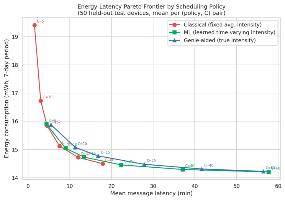
Figure 2.
Energy saving of the learned and genie-aided policies relative to the classical baseline, interpolated at matched mean latency from the Pareto frontiers in Figure 1.
Figure 2.
Energy saving of the learned and genie-aided policies relative to the classical baseline, interpolated at matched mean latency from the Pareto frontiers in Figure 1.
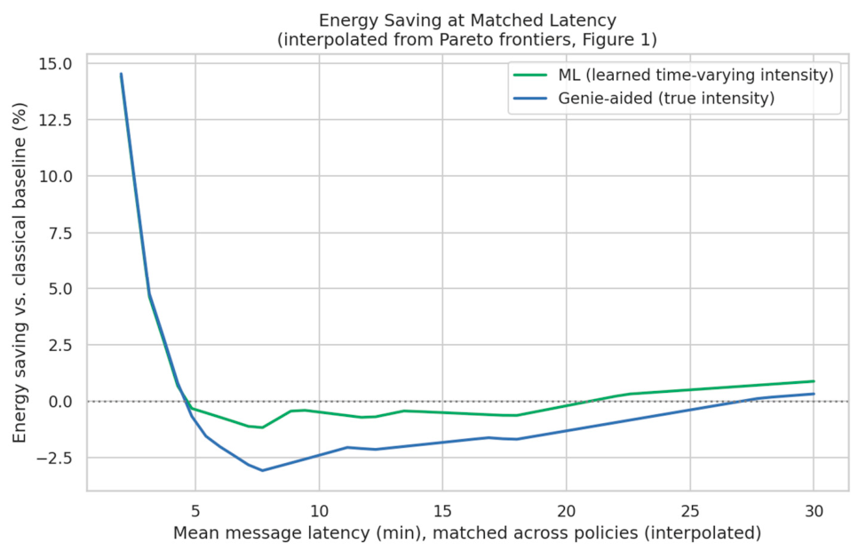
Figure 3.
Energy versus 95th-percentile (tail) message latency by scheduling policy (50 held-out test devices; mean per policy/C pair).
Figure 3.
Energy versus 95th-percentile (tail) message latency by scheduling policy (50 held-out test devices; mean per policy/C pair).
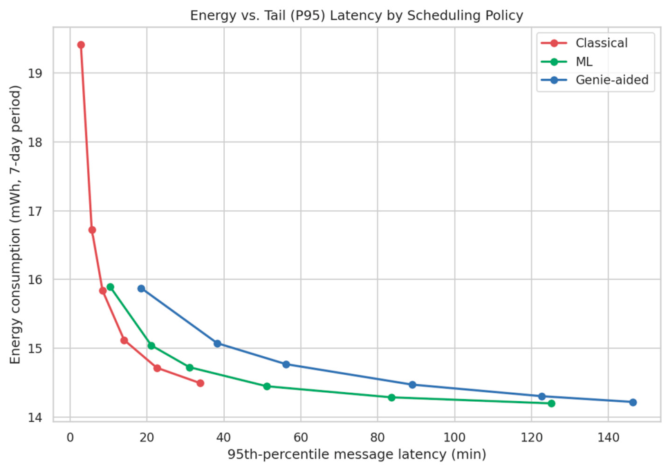
Figure 4.
True versus learned versus classical intensity estimate over an example 7-day held-out device trace.
Figure 4.
True versus learned versus classical intensity estimate over an example 7-day held-out device trace.
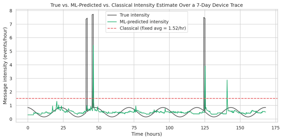
Figure 5.
Standard deviation of the true beam-slot arrival time versus the target beam index (3000 simulated sweep cycles per beam index), compared with the theoretical square-root-of-position scaling for accumulated independent per-beam jitter.
Figure 5.
Standard deviation of the true beam-slot arrival time versus the target beam index (3000 simulated sweep cycles per beam index), compared with the theoretical square-root-of-position scaling for accumulated independent per-beam jitter.
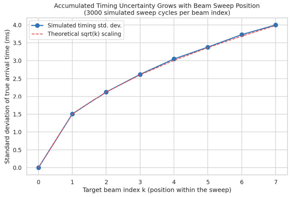
Figure 6.
Energy–reliability Pareto frontier for the three listen-window policies (150 simulated devices, 55 sweep cycles each).
Figure 6.
Energy–reliability Pareto frontier for the three listen-window policies (150 simulated devices, 55 sweep cycles each).
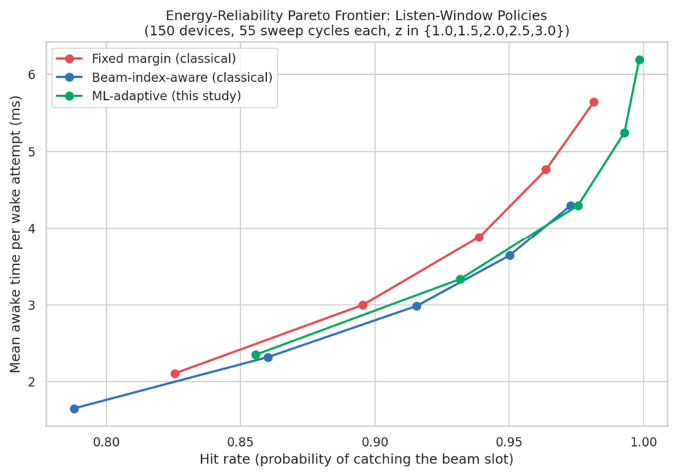

Table 1.
Hit rate and mean awake time per wake attempt by policy and margin multiplier z (150 simulated devices, 55 sweep cycles each).
Table 1.
Hit rate and mean awake time per wake attempt by policy and margin multiplier z (150 simulated devices, 55 sweep cycles each).
| z | Fixed: Hit / Awake (ms) | Beam-Aware: Hit / Awake (ms) | ML: Hit / Awake (ms) |
| 1.0 | 0.826 / 2.11 | 0.788 / 1.65 | 0.856 / 2.35 |
| 1.5 | 0.896 / 3.00 | 0.860 / 2.32 | 0.932 / 3.33 |
| 2.0 | 0.939 / 3.88 | 0.916 / 2.98 | 0.976 / 4.30 |
| 2.5 | 0.964 / 4.76 | 0.950 / 3.64 | 0.993 / 5.25 |
| 3.0 | 0.982 / 5.64 | 0.973 / 4.30 | 0.998 / 6.19 |
Disclaimer/Publisher’s Note: The statements, opinions and data contained in all publications are solely those of the individual author(s) and contributor(s) and not of MDPI and/or the editor(s). MDPI and/or the editor(s) disclaim responsibility for any injury to people or property resulting from any ideas, methods, instructions or products referred to in the content. |
© 2026 by the authors. Licensee MDPI, Basel, Switzerland. This article is an open access article distributed under the terms and conditions of the Creative Commons Attribution (CC BY) license.
Copyright: This open access article is published under a Creative Commons CC BY 4.0 license, which permit the free download, distribution, and reuse, provided that the author and preprint are cited in any reuse.