Genetic Geometry: A Unified View of Genome-Wide Association Studies and LD Score Regression

1. Introduction

LD Score regression was introduced by Bulik-Sullivan et al. [1] to distinguish inflation in genome-wide association study (GWAS) test statistics arising from polygenic signals from that arising from confounding, by examining the relationship between test statistics and linkage disequilibrium (LD). The quantities entering this relationship, however, arise from apparently different mathematical constructions. GWAS association reflects the relationship between genetic variation and phenotype, whereas the LD Score of a locus is constructed from correlations among genetic variants. A direct geometric connection between these quantities is therefore not immediately apparent. Here, we show that they can be represented within a common geometric framework.

LD Score and GWAS association statistics are therefore closely connected empirically. However, their mathematical definitions appear quite different. LD Score is defined from pairwise correlations among genetic variants, whereas a GWAS statistic is derived from the relationship between a genotype and a phenotype. It is therefore not immediately obvious why these two quantities can be related through regression. Genetic association can also be formulated using kernel-based representations. The sequence kernel association test (SKAT), for example, tests the association between a set of genetic variants and a phenotype using a kernel-based framework [2]. Previous work further showed that kernel statistics based on genetic relationship and identity-by-state matrices can be decomposed into calculations involving genotype-value vectors, providing a direct vector representation of genetic association statistics [3]. These observations suggest that vector and matrix representations may provide a useful framework for examining the relationship between genetic association and LD-based quantities. This apparent difference raises a more fundamental question: do LD Score and GWAS association statistics describe different structures, or are they different representations of quantities defined in a common genetic space?

In this study, we address this question by representing SNPs as vectors in the sample space and considering the eigenspace generated by these vectors. Each SNP vector can be expressed as a linear combination of a common set of orthogonal eigenvectors. The component of the phenotype vector contained in the same SNP space can likewise be represented using the same eigenvectors. Consequently, LD Score and phenotype association can both be expressed using coordinates defined with respect to a common eigenbasis. We refer to this representation as Genetic Geometry. This framework provides a unified view of genome-wide association studies and LD Score regression and allows their relationship to be examined within a single geometric coordinate system.

2. Theory

2.1. Vector Representation of Genetic Variants

Vector representations of genotype information have previously been used to decompose genetic relationship and identity-by-state kernel statistics [3]. Here, we use a related vector representation at the level of individual loci.

Consider L genetic loci measured in the same set of samples. For each locus i, we represent the standardized genotype by a unit vector $u_i$ in the sample space. Because the genotype vectors are centered and normalized, the correlation coefficient between loci i and j can be written as their inner product,

$$r_{ij}=u_i^T{u}_j.$$

(1)

Geometrically, this can also be written as

$$r_{ij}=cos{\theta }_{ij},$$

(2)

where ${\theta }_{ij}$ is the angle between $u_i$ and $u_j$. Thus, linkage disequilibrium can be interpreted geometrically in terms of the relative directions of genotype vectors in the sample space.

2.2. LD Score as a Quadratic Form

The LD Score of locus i is defined as

$${\ell }_i={\displaystyle \sum _{j=1}^L}{r}_{ij}^2.$$

(3)

Using the vector representation above,

$${\ell }_i={\displaystyle \sum _{j=1}^L}{\left(u_i^T{u}_j\right)}^2.$$

(4)

Because

$${\left(u_i^T{u}_j\right)}^2=u_i^T\left(u_j{u}_j^T\right)u_i,$$

(5)

the LD Score can be written as

$${\ell }_i=u_i^T\left({\displaystyle \sum _{j=1}^L}{u}_j{u}_j^T\right)u_i.$$

(6)

We define

$$A={\displaystyle \sum _{j=1}^L}{u}_j{u}_j^T.$$

(7)

The LD Score is therefore the quadratic form

$${\ell }_i=u_i^{T}A{u}_i.$$

(8)

The matrix A is symmetric and positive semidefinite and describes the structure generated by the genotype vectors in the sample space.

2.3. Spectral Representation of the SNP Space

Because A is symmetric and positive semidefinite, it can be decomposed into orthonormal eigenvectors $q_k$ and corresponding nonnegative eigenvalues ${\lambda }_k$,

$$A{q}_k={\lambda }_k{q}_k,$$

(9)

with

$$q_k^T{q}_l={\delta }_{kl}.$$

(10)

The spectral decomposition of A is therefore

$$A=\sum _k{\lambda }_k{q}_k{q}_k^T,$$

(11)

where the summation is taken over eigenvectors associated with nonzero eigenvalues.

The space spanned by these eigenvectors is identical to the space spanned by the genotype vectors $u_i$. Consequently, each genotype vector can be expanded in this common orthogonal basis. We write

$$u_i=\sum _k{a}_{ik}{q}_k,$$

(12)

where

$$a_{ik}=q_k^T{u}_i$$

(13)

is the coordinate of locus i along the kth eigenvector.

Substitution into the quadratic-form representation of the LD Score gives

$${\ell }_i={\left(\sum _k{a}_{ik}{q}_k\right)}^T\left(\sum _l{\lambda }_l{q}_l{q}_l^T\right)\left(\sum _m{a}_{im}{q}_m\right).$$

(14)

Using the orthogonality of the eigenvectors, this reduces to

$${\ell }_i=\sum _k{\lambda }_k{a}_{ik}^2.$$

(15)

Thus, the LD Score can be interpreted as the sum of the squared coordinates of a genotype vector in the common eigenspace, weighted by the corresponding eigenvalues.

2.4. Representation of the Phenotype in the Same Eigenspace

Let y denote a centered phenotype vector defined for the same samples. In general, y does not necessarily lie entirely in the space spanned by the genotype vectors.

We therefore decompose y into a component contained in the SNP space and a component e orthogonal to that space,

$$y=(y-e)+e,$$

(16)

where

$$e^T{q}_k=0$$

(17)

for every eigenvector $q_k$ spanning the SNP space.

Because $y-e$ belongs to the same space as the genotype vectors, it can be expanded using exactly the same eigenvectors,

$$y-e=\sum _k{b}_k{q}_k,$$

(18)

where

$$b_k=q_k^T(y-e).$$

(19)

Since $e^T{q}_k=0$, we also have

$$b_k=q_k^{T}y.$$

(20)

The genotype vector and the component of the phenotype contained in the SNP space can therefore be represented in the same coordinate system,

$$u_i=\sum _k{a}_{ik}{q}_k,y-e=\sum _k{b}_k{q}_k.$$

(21)

This common representation is central to the Genetic Geometry framework considered here.

2.5. Association in the Common Eigenspace

Because e is orthogonal to the SNP space,

$$e^T{u}_i=0.$$

(22)

Consequently,

$$y^T{u}_i={(y-e)}^T{u}_i.$$

(23)

Substituting the two eigenvector expansions gives

$$y^T{u}_i={\left(\sum _k{b}_k{q}_k\right)}^T\left(\sum _l{a}_{il}{q}_l\right).$$

(24)

Using $q_k^T{q}_l={\delta }_{kl}$,

$$y^T{u}_i=\sum _k{a}_{ik}{b}_k.$$

(25)

The squared association can therefore be written as

$${\left(y^T{u}_i\right)}^2={\left(\sum _k{a}_{ik}{b}_k\right)}^2.$$

(26)

The squared phenotype–genotype association can also be expressed as a quadratic form of the genotype vector. Because the component e is orthogonal to the SNP space, we have

$${\left(y^T{u}_i\right)}^2={\left[{(y-e)}^T{u}_i\right]}^2.$$

(27)

We define the phenotype-derived matrix

$$B=(y-e){(y-e)}^T.$$

(28)

Then,

$${\left(y^T{u}_i\right)}^2=u_i^{T}B{u}_i.$$

(29)

Thus, phenotype–genotype association and LD Score can both be expressed as quadratic forms of the same locus-specific genotype vector $u_i$. Specifically,

$${\left(y^T{u}_i\right)}^2=u_i^{T}B{u}_i,$$

(30)

where B is derived from the phenotype component contained in the SNP space, whereas

$${\ell }_i=u_i^{T}A{u}_i,$$

(31)

where A is derived from the genotype vectors across loci. The two quantities therefore share the same quadratic-form structure and differ in the matrix acting on $u_i$.

2.6. A Unified Representation of GWAS and LD Score Regression

The preceding derivations express the two locus-specific quantities in a common eigenspace. For locus i, the LD Score is

$${\ell }_i=\sum _k{\lambda }_k{a}_{ik}^2,$$

(32)

whereas the squared phenotype–genotype inner product is

$${\left(y^T{u}_i\right)}^2={\left(\sum _k{a}_{ik}{b}_k\right)}^2.$$

(33)

These expressions show that the two quantities are not constructed in unrelated spaces. Both depend on the same locus-specific coordinates $a_{ik}$ defined with respect to the same orthogonal basis $q_k$.

The LD Score weights the squared coordinates $a_{ik}^2$ by the eigenvalues ${\lambda }_k$ of the genotype-derived matrix A. In contrast, phenotype association combines the same coordinates $a_{ik}$ with the phenotype coordinates $b_k$ in the same eigenspace.

Thus, genome-wide association and LD Score regression can be viewed as different operations performed within a common genetic eigenspace. We refer to this common geometric representation as Genetic Geometry.

3. Numerical Simulation

3.1. Simulation Design

We performed a small numerical simulation to verify the spectral representation proposed in Genetic Geometry. A synthetic genotype matrix consisting of 40 samples and 60 biallelic loci was generated. The loci were divided into three blocks of 20 loci. Within each block, a common binary allele pattern was first generated, and individual loci were produced by randomly altering this pattern with increasing probabilities. The resulting dataset therefore contained groups of correlated loci, providing a simple LD-like structure.

This simulation was not intended to reproduce an explicit population genetic process such as recombination or a genealogical model. Rather, it was designed to provide a controlled genotype matrix containing nontrivial correlations among loci.

For each locus, the binary genotype vector was centered and normalized to unit length to obtain $u_i$. The pairwise correlation between loci i and j was calculated as

$$r_{ij}=u_i^T{u}_j.$$

(34)

The conventional LD Score was then calculated directly as

$${\ell }_i^{\mathrm{direct}}=\sum _j{r}_{ij}^2.$$

(35)

Independently, the matrix

$$A=\sum _j{u}_j{u}_j^T$$

(36)

was constructed and spectrally decomposed as

$$A=\sum _k{\lambda }_k{q}_k{q}_k^T.$$

(37)

Each SNP vector was expressed in this common eigenbasis as

$$u_i=\sum _k{a}_{ik}{q}_k.$$

(38)

The LD Score was then independently calculated from the spectral representation as

$${\ell }_i^{\mathrm{spectral}}=\sum _k{\lambda }_k{a}_{ik}^2.$$

(39)

3.2. Simulation of a Phenotype Vector

To examine the corresponding representation of phenotype association, a synthetic phenotype vector was constructed from components both within and outside the SNP space.

The SNP-space component of the phenotype was defined using the first three eigenvectors as

$$y-e=1.20q_1-0.80q_2+0.55q_3.$$

(40)

An additional random vector was generated and its projection onto the SNP space was removed. This produced a residual component e satisfying

$$e^T{q}_k=0$$

(41)

for every eigenvector spanning the SNP space.

The complete phenotype vector was then defined as

$$y=(y-e)+e.$$

(42)

For each locus, the squared phenotype–genotype association was calculated directly as

$$s_i^{\mathrm{direct}}={\left(y^T{u}_i\right)}^2.$$

(43)

Using the common eigenbasis,

$$y-e=\sum _k{b}_k{q}_k$$

(44)

and

$$u_i=\sum _k{a}_{ik}{q}_k,$$

(45)

the same quantity was independently calculated as

$$s_i^{\mathrm{spectral}}={\left(\sum _k{a}_{ik}{b}_k\right)}^2.$$

(46)

3.3. Numerical Verification

The direct and spectral calculations were compared for all loci. For the LD Score, the conventional calculation

$${\ell }_i^{\mathrm{direct}}=\sum _j{\left({\mathbf{u}}_i^T{\mathbf{u}}_j\right)}^2$$

(47)

was compared with the spectral representation

$${\ell }_i^{\mathrm{spectral}}=\sum _k{\lambda }_k{a}_{ik}^2.$$

(48)

The two calculations agreed to numerical precision for all loci, confirming the identity derived in Eq. (34). Thus, the LD Score calculated from pairwise correlations among SNPs can equivalently be calculated from the coordinates of each SNP in the common eigenbasis and the corresponding eigenvalues.

For phenotype–genotype association, the direct calculation

$$s_i^{\mathrm{direct}}={\left({\mathbf{y}}^T{\mathbf{u}}_i\right)}^2$$

(49)

was compared with the spectral representation

$$s_i^{\mathrm{spectral}}={\left(\sum _k{a}_{ik}{b}_k\right)}^2.$$

(50)

Again, the two calculations agreed to numerical precision for all loci, numerically confirming the representation derived in Eq. (41). The component of the phenotype orthogonal to the SNP space did not contribute to the phenotype–genotype inner product, as expected from Eq. (22).

Together, these results verify that both quantities can be calculated using the common eigenbasis of the SNP space. The numerical agreement does not represent an empirical approximation: it confirms the mathematical identities derived in the preceding sections. The relationship between the two distinct locus-specific quantities, ${\ell }_i$ and ${\left({\mathbf{y}}^T{\mathbf{u}}_i\right)}^2$, is examined separately in the graphical analysis below.

3.4. Graphical Verification

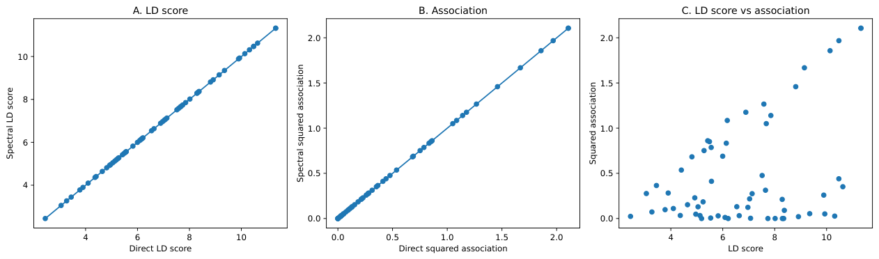
The numerical results were visualized in three complementary ways (Figure 1).

Panel A compares the LD Score calculated directly from pairwise correlations,

$${\ell }_i^{\mathrm{direct}}=\sum _j{\left(u_i^T{u}_j\right)}^2,$$

(51)

with the LD Score calculated from the spectral representation,

$${\ell }_i^{\mathrm{spectral}}=\sum _k{\lambda }_k{a}_{ik}^2.$$

(52)

Because the two expressions are mathematically identical, the points are expected to lie on the identity line.

Panel B compares the squared phenotype–genotype association calculated directly,

$$s_i^{\mathrm{direct}}={\left(y^T{u}_i\right)}^2,$$

(53)

with the corresponding quantity calculated in the common eigenspace,

$$s_i^{\mathrm{spectral}}={\left(\sum _k{a}_{ik}{b}_k\right)}^2.$$

(54)

Again, the two quantities are mathematically identical and therefore are expected to lie on the identity line.

Panel C directly compares the two locus-specific quantities of principal interest,

$${\ell }_i$$

(55)

and

$${\left(y^T{u}_i\right)}^2.$$

(56)

Unlike Panels A and B, there is no mathematical identity requiring the points in Panel C to lie on a straight line. This panel therefore visualizes the relationship between LD Score and phenotype association in the simulated genetic space. In the present simulation, the phenotype component within the SNP space was constructed from the first three eigenvectors. Consequently, Panel C illustrates one particular phenotype geometry rather than a general property of LD Score regression.

4. Discussion

In this study, we showed that genome-wide association studies (GWAS) and LD Score regression can be represented within the same genetic vector space. Although LD Score and phenotype–genotype association are conventionally introduced as different quantities, both can be expressed using coordinates defined with respect to the same orthogonal eigenvectors. Specifically, for locus i,

$${\ell }_i=\sum _k{\lambda }_k{a}_{ik}^2,$$

(57)

whereas

$${\left({\mathbf{y}}^T{\mathbf{u}}_i\right)}^2={\left(\sum _k{a}_{ik}{b}_k\right)}^2.$$

(58)

Although these two expressions involve different operations, they share the same locus-specific coordinates $a_{ik}$ defined in the common eigenbasis of the SNP space. The difference lies in how these coordinates are combined. The LD Score depends quadratically on the coordinates and weights them by the eigenvalues ${\lambda }_k$, whereas phenotype–genotype association depends on the inner product between the genotype coordinates $a_{ik}$ and the phenotype coordinates $b_k$.

This distinction is important for interpreting the present framework. The common eigenspace representation does not by itself imply a linear relationship between the LD Score and the squared phenotype–genotype association at individual loci. Such a relationship would require additional assumptions concerning the distribution of the phenotype coordinates and their relationship to the genetic structure. Rather, the result established here is more fundamental: the quantities entering GWAS association and LD Score can be expressed using coordinates in the same underlying genetic space.

The spectral representation also provides a geometric interpretation of LD structure. The eigenvectors of the matrix

$$\mathbf{A}=\sum _j{\mathbf{u}}_j{\mathbf{u}}_j^T$$

(59)

define orthogonal directions of genetic variation in the sample space, whereas the corresponding eigenvalues quantify the contribution of these directions to the genotype-derived structure. A SNP with a large coordinate along an eigenvector associated with a large eigenvalue makes a correspondingly large contribution to its LD Score. Thus, the LD Score can be interpreted not only as a sum of squared pairwise correlations, but also as a weighted measure of the position of a SNP within the spectral geometry generated by all genotype vectors.

The phenotype can be incorporated into exactly the same coordinate system. Only the component of the phenotype contained in the SNP space contributes to its inner product with a genotype vector, because the orthogonal component has zero inner product with every SNP vector. The association between a phenotype and a locus can therefore be interpreted as an alignment between the coordinate vector of the locus and the coordinate vector of the phenotype within the genetic eigenspace.

The numerical simulation illustrates these identities directly. The conventional calculation of LD Score from pairwise SNP correlations and its spectral representation give the same quantity. Likewise, the direct phenotype–genotype inner product and its expression in the common eigenbasis represent the same association quantity. These agreements follow from the mathematical identities derived above and serve as a numerical verification of their implementation.

The present analysis has several limitations. First, the simulated genotype data were designed to contain a simple correlation structure and were not generated from an explicit population-genetic model. Second, the phenotype was constructed from selected eigenvectors in order to demonstrate the geometry of phenotype association. Therefore, the relationship between LD Score and phenotype association observed in this simulation should not be interpreted as a general model of complex trait architecture. Third, the present study establishes a common coordinate representation but does not derive the statistical expectation underlying conventional LD Score regression.

These limitations also suggest a natural direction for further work. The Genetic Geometry framework separates two components that are often considered through different mathematical formulations: the geometry of genetic variation, represented by ${\lambda }_k$ and $a_{ik}$, and the location of a phenotype within the same space, represented by $b_k$. Investigating statistical models for the phenotype coordinates $b_k$ may provide a direct route from this geometric representation to the expected relationship between association statistics and LD Score.

5. Conclusion

We have shown that LD Score and phenotype–genotype association can be represented within a common eigenspace generated by standardized genotype vectors. In this representation, the LD Score of locus i is

$${\ell }_i=\sum _k{\lambda }_k{a}_{ik}^2,$$

(60)

whereas the squared phenotype–genotype association is

$${\left({\mathbf{y}}^T{\mathbf{u}}_i\right)}^2={\left(\sum _k{a}_{ik}{b}_k\right)}^2.$$

(61)

Both quantities therefore depend on the same locus-specific coordinates $a_{ik}$, while differing in how these coordinates are combined with the genetic eigenvalues or phenotype coordinates. This common representation provides a geometric connection between quantities used in GWAS and LD Score regression without assuming that their locus-specific values are identical or necessarily proportional

References

- Bulik-Sullivan, B. K.; Loh, P.-R.; Finucane, H. K.; Ripke, S.; Yang, J. Schizophrenia Working Group of the Psychiatric Genomics Consortium LD Score regression distinguishes confounding from polygenicity in genome-wide association studies. In Nature Genetics; Patterson, N., Daly, M. J., Price, A. L., Neale, B. M., Eds.; 2015; Volume 47, pp. 291–295. [Google Scholar] [CrossRef] [PubMed]
- Wu, M.C.; Lee, S.; Cai, T.; Li, Y.; Boehnke, M.; Lin, X. Rare-variant association testing for sequencing data with the Sequence Kernel Association Test. Am. J. Hum. Genet. 2011, 89, 82–93. [Google Scholar] [CrossRef] [PubMed]
- Misawa, K. Genotype Value Decomposition: Simple Methods for the Computation of Kernel Statistics. Adv. Genet. 2022, 3, 2100066. [Google Scholar] [CrossRef] [PubMed]
Figure 1.
Numerical verification of Genetic Geometry using simulated genotype and phenotype data. (A) Comparison between LD Scores calculated directly as and those calculated from the spectral representation as . The diagonal line represents equality between the two calculations. (B) Comparison between squared phenotype–genotype associations calculated directly as and those calculated in the common eigenspace as . The diagonal line again represents equality. (C) Relationship between LD Score and squared phenotype–genotype association for each simulated locus. Unlike the comparisons in panels A and B, the quantities shown in panel C are not mathematically required to be identical. The phenotype used in this simulation contained components along the first three eigenvectors of the SNP space. Panel C is included as an exploratory visualization and is not intended to reproduce the statistical assumptions of conventional LD Score regression.
Disclaimer/Publisher’s Note: The statements, opinions and data contained in all publications are solely those of the individual author(s) and contributor(s) and not of MDPI and/or the editor(s). MDPI and/or the editor(s) disclaim responsibility for any injury to people or property resulting from any ideas, methods, instructions or products referred to in the content. |
© 2026 by the authors. Licensee MDPI, Basel, Switzerland. This article is an open access article distributed under the terms and conditions of the Creative Commons Attribution (CC BY) license (http://creativecommons.org/licenses/by/4.0/).
Copyright: This open access article is published under a Creative Commons CC BY 4.0 license, which permit the free download, distribution, and reuse, provided that the author and preprint are cited in any reuse.