

Submitted:
07 October 2026
Posted:
09 October 2026
You are already at the latest version
Abstract
Electromagnetic vibration energy harvesters with magnetic levitation are of interest for powering autonomous low-power devices due to their high output power; however, their narrow operating region makes them sensitive to changes in the parameters of external vibration excitation. This study investigates the effects of excitation frequency and base acceleration amplitude on the harvester’s output characteristics and evaluates mean power retention under combined deviations in these parameters. Numerical simulations of steady-state regimes were performed. Within prescribed neighborhoods of operating points, the minimum mean power and local relative power variation were determined. For the configuration considered, increasing the deviation bounds from ±0.2 Hz and ±0.2 g to ±0.8 Hz and ±0.8 g reduces the highest retained fraction of the global maximum power in the investigated domain from 77.73% to 24.58%, while the local relative power variation at the corresponding operating points increases from 16.46% to 66.48%. These results highlight the risk of selecting a high-power operating point near a sharp power-drop boundary, where excitation deviations can leave the load underpowered. The proposed analysis addresses this risk by evaluating the minimum mean power across the prescribed deviation range and identifying operating regions that satisfy the load’s power requirement.
Keywords:
electromagnetic vibration energy harvester
; magnetic levitation
; nonlinear resonance
; parametric analysis
; power retention
; local relative power variation
; operating region selection
1. Introduction
Wireless sensor nodes are widely used in industry for real-time remote monitoring of facilities, equipment, and industrial processes [1]. For the large-scale deployment of autonomous sensor systems, a reliable and long-term power supply remains one of the key challenges [2]. Regular replacement and maintenance of electrochemical batteries in distributed or hard-to-reach systems are technically challenging and costly [3].
A promising approach to providing autonomous power for sensors and low-power electronic devices is the conversion of ambient energy into electrical energy [3]. In industrial and transportation systems, the conversion of mechanical vibration energy is of particular interest, since vibrations often arise as a byproduct of the operation of machines, engines, structures, and process equipment [4,5]. The use of vibration energy harvesters can reduce dependence on batteries and extend the autonomous operating time of distributed sensor systems [6].
The main methods for converting mechanical energy into electrical energy include piezoelectric, electrostatic, and electromagnetic approaches [7,8,9]. In addition, hybrid solutions that combine several energy conversion mechanisms are being actively developed [10,11]. Electromagnetic transducers are of interest due to their relatively low internal resistance, the ability to generate a useful output current, and their structural simplicity [12,13]. Under low-frequency vibration excitation, the choice of the transducer’s suspension and mechanical structure—which determine its resonant characteristics—is of particular importance.
This study considers an electromagnetic vibration energy harvester with magnetic levitation. In this system, the restoring force is generated through magnetic interactions without mechanical contact, which can reduce the effects of wear and eliminate the need for a conventional elastic element. Furthermore, magnetic levitation gives rise to a nonlinear restoring force, which can significantly affect the device’s resonant behavior and energy output characteristics [13].
Under real operating conditions, the excitation frequency and base acceleration amplitude may vary over time [14]. For a harvester with a narrow region of high power output, such variations can shift the operating point outside this region and substantially reduce the power output. Therefore, high power output under a single fixed excitation condition does not characterize the device’s ability to maintain the required power level as the excitation conditions change. To support an informed selection of the operating regime, it is necessary to determine the minimum mean power retained within the expected deviation bounds for excitation frequency and base acceleration amplitude.
The objective of this study is to investigate the effects of vibration excitation frequency and base acceleration amplitude on the output characteristics of a magnetically levitated electromagnetic energy harvester. Based on a parametric analysis of steady-state regimes, mean power retention under deviations in these parameters is assessed to identify operating regions in which the minimum mean power meets the specified power requirement.
The main contributions of this work are as follows:
— The effects of excitation frequency and base acceleration amplitude on the load voltage and mean output power of the harvester were demonstrated.
— For the investigated harvester, a high nominal power was found to coexist with a low retained minimum when the prescribed frequency–acceleration neighborhood extended across the sharp power-drop boundary. This establishes the importance of the entire deviation neighborhood, rather than the nominal operating point alone, in assessing power availability.
— Based on this finding, a principle for selecting operating regions was formulated: the minimum mean power within the prescribed joint excitation deviations must satisfy the load’s power requirement, while local relative power variation is used to compare regions meeting this condition.
The paper is organized as follows. Section 2 reviews studies on magnetically levitated electromagnetic vibration energy harvesters and discusses the limitations of existing approaches. Section 3 presents the mathematical model and the methodology for the parametric analysis of the harvester’s steady-state output characteristics under harmonic excitation. Section 4 presents the simulation results for the device’s output voltage and mean power, together with assessments of power retention and local relative power variation under specified deviations in excitation frequency and base acceleration amplitude. Section 5 discusses the physical interpretation and practical implications of the results. Section 6 summarizes the main conclusions of the study.
2. Related Work
Electromagnetic vibration energy harvesters (EVEHs) differ in their kinematic arrangement, magnetic system configuration, and suspension type. In magnetically levitated designs, the restoring force is generated by magnetic interaction, which determines the device’s resonant characteristics [13].
The potential of such harvesters to power low-power devices has been investigated in various configurations. In [15], an electromagnetic harvester is used to extend the autonomous operating time of a wearable Internet of Things (IoT) device. Experimental prototypes demonstrate useful power generation both at frequencies of approximately 3–4 Hz and accelerations of around 0.4 g, where the output reaches tens of milliwatts [16], and at higher resonant frequencies [17]. In [18], a levitation-based harvester is combined with a sensor based on giant magnetoimpedance for energy harvesting and mechanical vibration sensing.
Reliable prediction of the behavior of magnetically levitated EVEHs requires coupled electromechanical models that account for the nonlinear magnetic restoring force, coil parameters, load resistance, and electromechanical coupling between the mechanical and electrical subsystems. In [19], a one-dimensional model was proposed in which nonlinearity is represented by the actual magnetic force relationship and position-dependent magnetic flux and electromotive force (EMF). The force and electromagnetic characteristics were validated by comparing numerical simulations with experimental results. In [20], a two-degree-of-freedom system with multiple moving magnets was investigated using a coupled electromechanical formulation. The study showed that magnetic nonlinearity can lead to complex motion regimes and that load parameters and electromechanical coupling coefficients significantly affect the current and output power. Thus, modern models of magnetically levitated EVEHs incorporate a nonlinear description of magnetic interaction, electrical circuit parameters, and experimental validation of numerical results.
The nonlinear dynamics of magnetically levitated EVEHs manifest as amplitude-dependent resonance, changes in effective stiffness, multistability, hysteresis, and abrupt transitions between oscillation regimes. These effects are important both for the physical description of the system and for the practical assessment of the robustness of its output characteristics to variations in excitation parameters and electrical load. Several studies consider the nonlinearity associated with magnetic levitation as a means of broadening the operating bandwidth and improving energy conversion efficiency [14,21]. In [22], an energy harvester based on diamagnetic levitation is presented for ultralow-frequency vibrations and human motion. In [23], a frequency-tunable electromagnetic vibration energy harvester based on diamagnetic levitation is investigated, demonstrating the potential to control resonant properties through the magnetic structure.
The literature places particular emphasis on the effects of magnetic nonlinearity on the shape of the frequency response and the emergence of multiple stable regimes. In [24], the nonlinear magnetic restoring force is shown to produce a softening effect, hysteresis, and multiple resonant response regimes during a frequency sweep. In [25], system nonlinearity is described by a polynomial magnetic force relationship that includes cubic and fifth-order terms, allowing the complex nature of magnetic interaction at finite displacements to be captured. In [26], magnetic levitation also gives rise to a nonlinear restoring force and multiple resonant response regimes that significantly affect the system’s dynamic response.
In our previous study [27], an experimentally validated nonlinear electromechanical model was used to examine how magnetic suspension characteristics influence the resonant response, output power, and power density of a magnetically levitated electromagnetic energy harvester. Variations in suspension geometry modified the magnetic restoring force and effective stiffness, providing a basis for configuration selection under prescribed harmonic excitation. The predicted high-power region was narrow in frequency, indicating sensitivity of the attainable output to deviations of the excitation frequency from resonance.
Active control strategies have also been developed to adapt energy harvesters to changing excitation conditions. Hara et al. [28] proposed a fuzzy-logic-based adaptive switching strategy for a piezoelectric energy harvester. Experiments demonstrated increased output voltage under frequency sweeps, changes in the number of dominant frequencies, and broadband vibrations.
The reviewed studies show that magnetic system design, electrical load parameters, and excitation conditions significantly affect the energy output characteristics of harvesters. However, achieving high power output at a specific combination of parameters does not establish how much power is retained when these parameters deviate from their nominal values. For a harvester with a narrow region of high power output, determining the minimum power level within the expected deviation bounds for excitation frequency and base acceleration amplitude is of practical importance. This assessment is necessary to identify operating regions that meet a specified power requirement.
In this study, this problem is addressed through a parametric analysis of steady-state regimes at fixed combinations of harmonic excitation frequency and base acceleration amplitude. For prescribed neighborhoods of operating points, the minimum mean power normalized to the global maximum power in the investigated parameter domain and the local relative power variation are determined. Considering these metrics together enables the assessment of the retained power level and output variability, as well as the identification of operating regions that meet the specified power requirement.
3. Model and Numerical Study Setup
The mathematical model, experimental prototype, and validation procedure for the magnetically levitated electromagnetic vibration energy harvester are described in detail in our previous study [27]. In the present study, this model is used for a parametric analysis of steady-state output characteristics at various combinations of excitation frequency and base acceleration amplitude. The main equations and assumptions underlying the numerical study are presented below.
3.1. Harvester Configuration and Electromechanical Model
The physical configuration and principal components of the harvester are shown in Figure 1. The device comprises a non-magnetic guide tube, two fixed permanent magnets positioned at its upper and lower ends, a moving permanent magnet located between them, and an induction coil surrounding the central region of the tube. The fixed magnets are oriented so that their poles facing the moving magnet produce repulsive interactions. These interactions provide the magnetic restoring force governing the axial motion of the moving element.
Figure 1a and Figure 1b show the internal arrangement and principal components of the harvester, while Figure 1c presents a photograph of the prototype mounted on a vibration shaker. The guide tube constrains the moving magnet primarily to motion along the common axis of the magnetic assembly and the coil. The fixed magnets and the coil are attached to the housing and move with the vibrating base. Base excitation produces relative motion between the moving magnet and the coil, changing the magnetic flux linked with the coil turns and inducing an electromotive force. When the coil is connected to an external load resistance RL, the induced current delivers electrical power to the load and produces an electromagnetic reaction force on the moving magnet.
To describe the axial motion of the moving magnet relative to the housing, the harvester is represented as a single degree of freedom mechanical system coupled to the coil–load circuit. The equation of motion accounts for mechanical damping, the nonlinear magnetic restoring force, electromagnetic feedback, and excitation due to base acceleration.
In general form, the equation of motion can be written as
where z is the displacement of the moving element, m is the equivalent mass, c is the damping coefficient, Fm(z) is the nonlinear magnetic restoring force, Fe(t) is the electromagnetic force associated with the energy conversion process and Fexc(t) is the external vibration excitation. The nonlinear nature of the magnetic force causes the system's dynamic response to depend on the oscillation amplitude and initial conditions, allowing for the existence of multiple steady-state regimes under identical excitation parameters.
3.2. Nonlinear Magnetic Restoring Force
In the magnetically levitated vibration energy harvester under study, the restoring force is generated through the interaction between the levitating and fixed permanent magnets. Unlike traditional linear elastic systems, such a force is not characterized by a constant stiffness coefficient over a wide range of displacements. Therefore, the magnetic restoring force is treated as a nonlinear function of the moving element's displacement.
In the present work, the magnetic restoring force is defined by an analytical expression describing its nonlinear dependence on the displacement z:
Here, Br is the residual magnetic induction of the magnet material, r is the radius (characteristic dimension) of the magnetic system, hm is the height (thickness) of the magnet, μ0 is the magnetic constant and z is the displacement of the moving element (the coordinate determining the relative position of the magnets). The resulting restoring force Fm(z) is defined as the difference between the forces generated by the lower and upper fixed magnets, each of which is calculated using expression (2) [27].
3.3. Electromechanical Coupling and Output Characteristics
Electromechanical coupling in the energy harvester under study arises from the relative motion between the levitating magnet and the induction coil. As the magnet moves, the magnetic flux linked with the coil turns changes, inducing an electromotive force in the electrical circuit. In the model employed, the induced EMF is assumed to be proportional to the relative velocity of the moving element:
where e(t) is the induced EMF, ke is the electromechanical coupling coefficient and is the relative velocity of the moving element. In the present model, the electromechanical coupling coefficient kₑ is assumed to be constant, corresponding to the approximation of a uniform magnetic flux distribution in the coil's working zone; a more precise dependence of kₑ on the position of the moving element is discussed in [27].
The electrical subsystem is represented by a coil with resistance and inductance connected to an external load resistance RL. The current in the circuit is determined by the equation of the electrical subsystem:
where Lc is the coil inductance, Rc is the coil resistance, RL is the load resistance and i(t) is the current in the circuit.
Lcdi(t)/dt + (Rc + RL)i(t) = e(t),
The electromagnetic reaction on the mechanical subsystem is accounted for by a force proportional to the current in the electrical circuit:
Fe(t) = kei(t)
Thus, the mechanical and electrical subsystems are coupled: the velocity of the moving element determines the induced EMF and the current in the circuit, while the current generates an electromagnetic force that affects the motion of the moving element.
The output characteristics considered are the load voltage and the average power delivered to the load. The voltage across the load is defined as
and the instantaneous power at the load:
uL(t) = RLi(t),
pL(t) = uL(t)i(t) = RLi2(t)
The average output power over a time interval T is calculated using the expression:
These quantities are used to evaluate the effect of excitation frequency and base acceleration amplitude on the output voltage and average power delivered to the load.
3.4. Specification of Harmonic Vibration Excitation
This study investigates the influence of vibration excitation parameters—specifically, the excitation frequency and the base acceleration amplitude —on the output characteristics of an energy harvester. In each individual calculation, the excitation is modeled as steady-state harmonic motion, with parameters varied across specified ranges between calculations; this approach enables an assessment of the sensitivity of the output characteristics to changes in the vibration conditions.
The external input acting on the moving element due to base vibration enters the equation of motion (1) via the force Fexc(t), which is related to the base acceleration ab(t) by the expression:
where m is the equivalent mass of the moving element.
Fexc(t) = −mab(t),
The base acceleration is defined by a steady-state harmonic law:
where Ab is the base acceleration amplitude and f is the excitation frequency.
ab(t) = Absin(2πft),
The parameters f and Ab are assumed constant within each calculation and are varied within specified ranges across a series of numerical simulations (see Section 3.5), enabling an assessment of the influence of excitation frequency and base acceleration amplitude on the output voltage and average load power.
3.5. Numerical Implementation and Calculation Protocol
The numerical study is conducted based on the model presented in Section 3.1, Section 3.2 and Section 3.3, using the harmonic excitation defined in Section 3.4. A separate time-domain calculation is performed for each combination of excitation frequency and base acceleration amplitude. The excitation parameters remain constant throughout each calculation. The geometric, mechanical, and electrical parameters of the harvester remain unchanged across the entire series of calculations.
The system of differential equations is integrated using the “solve_ivp” function from the SciPy library, employing the adaptive Runge–Kutta method of order 5(4) (RK45). All calculations start from identical initial conditions. The ranges for the frequency and base acceleration amplitude, as well as the computational grid steps, are provided in Section 3.6.
The duration of each simulation is 50 s. To exclude the initial transient response, the first 10 s of each time history are omitted from the analysis. The RMS load voltage and mean output power are evaluated over the interval from 10 to 50 s, corresponding to an averaging window of 40 s. The mean power delivered to the load is obtained by time-averaging the instantaneous power according to Equation (8).
The obtained values form a surface representing the dependence of average power on the excitation frequency and base acceleration amplitude. This surface is used to determine the minimum power and local relative power variation within specified neighborhoods of operating points, following the methodology described in Section 3.7.
3.6. Set of Parameters and Modeling Conditions
The main parameters of the energy harvester model are listed in Table 1. The nonlinear magnetic restoring force Fm(z) is defined by the analytical relationship given in Section 3.2.
The external input is defined as base vibration excitation and is characterized by the excitation frequency f and the base acceleration amplitude Ab. To evaluate the influence of the excitation parameters, calculations are performed across a specified frequency range and at several levels of base acceleration. The vibration excitation parameters are listed in Table 2.
The calculations consider steady-state harmonic excitation at various excitation frequencies and base acceleration amplitudes. The parameters of the energy harvester model and the electrical circuit remain constant; only the frequency and acceleration amplitude of the external vibration input are varied. This ensures a valid comparison of the output voltage and average load power under different vibration conditions.
3.7. Assessment of Power Retention and Local Relative Power Variation
To evaluate the effect of excitation parameter deviations, the average output power surface Pavg(f,Ab) is used. The load power is calculated from the steady-state response in accordance with expression (8). For each operating point, the minimum power within a specified neighborhood and the relative power variation within that neighborhood are determined.
The nominal power at an operating point with frequency f0 and base acceleration amplitude Ab0 is equal to
P0 = Pavg(f0,Ab0)
The neighborhood of the operating point is defined by fixed absolute deviation limits:
Ω(f0,Ab0) = {(f,Ab): |f − f0| ≤ hf, |Ab − Ab0| ≤ hA}
Here, hf = 0.2 Hz and hA = 0.2 g — are the limits of frequency and acceleration amplitude deviations used in constructing the maps in Section 4.3. These values define the dimensions of the neighborhood and do not represent the grid spacing. Region (12) encompasses all parameter combinations within the specified limits.
The minimum and maximum powers in the vicinity are determined by the expressions
The values and depend on the position of the neighborhood center. The global maximum over the entire parameter domain under investigation is used to normalize the minimum power:
The retained fraction of the total peak power is characterized by a dimensionless coefficient.
The local relative power variation is determined independently of the global maximum and normalized by the maximum power within the same neighborhood:
For non-negative power and positive denominators, the following conditions hold for neighborhoods Ω ⊆ : 0 ≤ Kglob ≤ 1 and 0 ≤ Dloc ≤ 1. The maps show values 100Kglob% and 100Dloc%, respectively. The coefficient Kglob characterizes the minimum power level relative to the global maximum, while Dloc — represents the relative difference in magnitudes within the neighborhood. When the local relative power variation is undefined.
In the numerical implementation, local extrema are determined based on the internal and boundary computational nodes within the neighborhood, while the global maximum is determined from the nodes of the entire region under study. Consistent conditions for isolating the steady-state response and averaging power are applied in all calculations. Estimating the full range of deviations requires coverage of the entire neighborhood (12) with computational data; truncating this coverage at the boundary of the region under study alters the deviation limits being considered. The resulting extrema pertain to the computational grid and do not define values between its nodes.
The assessment is deterministic and pertains to steady-state conditions obtained using the adopted calculation protocol and specified initial conditions. Probabilistic parameter distributions are not introduced. Changes in power resulting from rapid, time-varying changes in excitation require a separate dynamic analysis.
4. Results
4.1. Basic Characteristics Under Steady-State Excitation
This section examines the basic harmonic excitation regime with a fixed base acceleration amplitude. The 20-second time-history record encompasses both the initial transient process and the subsequent steady-state response. The complete record allows for the observation of the oscillation build-up, while the quantitative characteristics of the regime are determined from its steady-state segment in accordance with Section 3.5. The values obtained are used for the subsequent comparison of regimes across various frequencies and base acceleration amplitudes.
Calculations are performed for a specified load resistance of RL = 1 Ω. The excitation frequency f is varied within the 7–13 Hz range, covering the device's resonance region and adjacent sections of the frequency response.
Figure 2 shows the frequency dependence of the load RMS voltage URMS(f), obtained during the specified frequency sweep. From this characteristic, the resonant frequency fr = 10.8 Hz is determined, at which the maximum voltage URMS,max = 72.60 mV. The corresponding average power delivered to the load is Pavg,max = 5.27 mW.
The obtained frequency response serves as a baseline for the subsequent comparison of steady-state output characteristics at various frequencies and amplitudes of base acceleration. Next, the dynamic response of the system at the identified resonant point fr is examined.
To illustrate the steady-state regime, Figure 3a shows the time-domain waveform of the induced EMF at the resonant frequency fr, demonstrating the initial transient process and the subsequent establishment of oscillations. The signal is quasi-harmonic in nature; however, due to nonlinear magnetic interaction, its shape may deviate from an ideal sinusoid. To monitor the dynamic regime, Figure 3b presents the phase portrait of the moving element's motion z – : the closed trajectory indicates a steady-state periodic oscillation regime. The nonlinear nature of the response is further evidenced by the frequency content of the output signal: Figure 3c shows the amplitude spectrum of the induced EMF, where, in addition to the fundamental component at the excitation frequency, extra harmonic components are observed—a result of the nonlinear form of the magnetic restoring force.
4.2. Output Power Response Surface with Respect to Excitation Frequency and Base Acceleration Amplitude
To evaluate the dependence of the average output power on the excitation parameters, a series of calculations was performed using various combinations of frequency f and base acceleration amplitude Ab. For each combination, the average power was determined from the steady-state portion of the time-domain signal in accordance with Section 3.5.
The calculations yielded a response surface Pavg(f, Ab), representing the dependence of the average output power on the excitation frequency and the base acceleration amplitude. Figure 4 shows the output power dependence obtained by varying both parameters.
Figure 4 shows that maximum average output power values occur within a limited range of the parameters f and Ab. As one moves away from this region, the values Pavg decrease. The maxima of the frequency profiles at various base acceleration amplitudes form a distinct resonant ridge.
At the lower end of the investigated acceleration range Ab = 0.5 g, the power maximum occurs at a frequency of 10.2 Hz. At a higher acceleration of Ab = 2.1 g, the maximum is reached at 12.2 Hz. The corresponding average power values are 2.86 mW and 12.49 mW. Between these points, a sequence of maxima appears at intermediate acceleration levels, forming a sloping ridge on the surface. As acceleration increases, the position of the ridge shifts toward higher frequencies.
At the same time, the increase in power is not solely a function of acceleration amplitude. For identical values of Ab, the output power can vary significantly depending on the excitation frequency. Maximum power values are observed in the region close to the system's resonant frequency, where the energy of the external vibration is most efficiently transferred to the levitating magnet. As the frequency deviates from this region, the output power decreases, even if the acceleration amplitude remains sufficiently high.
The power variation exhibits markedly different characteristics on either side of the ridge. Moving away from the maximum toward lower frequencies, the power declines gradually, forming an extended low-frequency slope. On the high-frequency side, the drop is much sharper: within a narrow frequency interval, the surface transitions from high power values to significantly lower ones. This transition creates a distinct, steep edge adjacent to the resonant ridge. As base acceleration increases, a rise in power is observed across the response surface. In the low-frequency region, this increase occurs gradually, whereas near the steep edge, there is an abrupt transition from low to high power values.
4.3. Power Retention and Selection of Operating Ranges
Section 4.2 establishes that high output power values are concentrated within a limited range of frequencies and base accelerations. The study further examines how the minimum power within a given neighborhood varies depending on the operating point's position relative to the resonance ridge and the region of sharp power drop-off. The results are presented as complementary maps showing the retained fraction of the overall maximum power and the local relative power variation.
Figure 5 shows the distribution of the minimum average power in the vicinity of each operating point, given frequency deviations of ±0.2 Hz and base acceleration amplitude deviations of ±0.2 g. The values are normalized to the maximum power across the entire investigated range and expressed as percentages. Elevated values form a band that shifts toward higher frequencies as the base acceleration increases. The highest values shown occur at a frequency of approximately 11.7–11.8 Hz and a base acceleration of 2.0–2.1 g. As the acceleration decreases, the peak values of the parameter within the corresponding frequency ranges also decrease.
The frequency distribution of the parameter exhibits marked asymmetry. As the frequency approaches the maximum from the low-frequency side, the retained power fraction gradually increases. At a base acceleration of approximately 2.0–2.1 g, the minimum power in the vicinity of the operating point is about 31% of the overall maximum at a frequency of 10.0 Hz, and about 54% at 11.0 Hz.
A sharp drop in the parameter is observed on the high-frequency side of the peak. At the same acceleration level, the retained power fractions for operating points with frequencies around 11.8 and 12.0 Hz are approximately 78% and 3%, respectively. Thus, a frequency shift of the neighborhood center by approximately 0.2 Hz is accompanied by a decrease in the parameter of about 75 percentage points. This transition defines a distinct high-frequency edge of the band characterized by elevated retained power.
At the most favorable operating point, the minimum power within the specified deviations is approximately 77.7% of the overall maximum—falling about 22.3% below it. Beyond the high-frequency side of the identified boundary, the minimum power remains at a level of only a few percent of the overall maximum.
Figure 6 shows the distribution of the local relative variation in average power given deviations of ±0.2 Hz in frequency and ±0.2 g in base acceleration amplitude. This metric is defined as the difference between the maximum and minimum power within each neighborhood, normalized by its local maximum. It complements the power-retention map by characterizing the variability of the energy output within the specified parameter deviations.
A band of elevated local relative power variation, with values of approximately 97%, stands out on the map. As the base acceleration increases, this band shifts toward higher frequencies: at Ab=0.5 g it spans the 10.2–10.8 Hz range, whereas at Ab=2.1 g — it covers approximately 12.0–12.4 Hz. On the high-frequency side of the band, the local relative power variation decreases. Specifically, at Ab=2.1g the values drop from 61.45% at 12.6 Hz to 46.20% at 13.0 Hz.
A comparison of Figure 5 and Figure 6 reveals that the highest retained fraction of the global power maximum on the computational grid is 77.73%, achieved at a frequency of 11.8 Hz and a base acceleration of 2.1 g. The local relative power variation in the vicinity of this point is 16.46%. At the same acceleration but a frequency of 12.0 Hz, the retained fraction drops to 3.02%, while the local relative power variation rises to 96.98%. Thus, adjacent operating points differ significantly in terms of both the minimum retained power level and its variability within the specified parameter deviations.
At the lower end of the acceleration range, a low level of retained power is accompanied by significant local relative power variation. At a base acceleration of 0.5 g and frequencies of 7.0 and 13.0 Hz, the retained fraction of the overall maximum is less than 1%, whereas the local relative power variation amounts to 73.78% and 61.85%, respectively. Consequently, in these low-power regions, low absolute power values are not accompanied by low local relative power variation.
To assess the effect of neighborhood size, results were additionally compared across four combinations of limiting deviations for frequency and base acceleration. Table 3 presents the maximum retained fraction of the total peak power for each range considered. These values were obtained by separately identifying the maximum retention coefficient across operating points for each neighborhood size.
Widening the limits of frequency and acceleration deviations is accompanied by a substantial reduction in the maximum retained power. When shifting from ±0.2 Hz and ±0.2 g to ±0.8 Hz and ±0.8 g, this share decreases from approximately 77.73% to 24.58% of the overall maximum—a roughly 3.2-fold reduction. For the intermediate ranges of ±0.4 Hz and ±0.4 g, as well as ±0.6 Hz and ±0.6 g, the values are 57.58% and 39.71%, respectively. These figures were obtained by selecting, for each deviation range, the specific operating point that yields the highest retention factor.
At the selected operating points, the local relative power variation increases from 16.46% to 66.48%. For the intermediate ranges of ±0.4 Hz and ±0.4 g, as well as ±0.6 Hz and ±0.6 g, the values are 33.24% and 50.15%, respectively. Thus, across the sequence of ranges considered, the decrease in the maximum retained power fraction is accompanied by an increase in local relative power variation at the selected points. At the smallest deviations, a retained fraction of 77.73% corresponds to a local relative power variation of 16.46%, whereas at the largest deviations, the respective values are 24.58% and 66.48%.
When the requirement is to retain at least 70% of the total maximum power, suitable operating points exist only for the narrowest of the considered ranges—±0.2 Hz and ±0.2 g. At the point with the highest retention ratio, this range corresponds to a local relative power variation of 16.46%. When the required fraction is reduced to 50%, the condition is also met for deviations of ±0.4 Hz and ±0.4 g: the retained fraction is 57.58%, and the local relative power variation at the corresponding point is 33.24%. For the two wider ranges, even the highest retained power fractions—39.71% and 24.58%—remain below the specified level.
5. Discussion
5.1. Physical Interpretation of the Obtained Results
In a magnetically levitated electromagnetic vibration energy harvester, the energy of base vibrations is converted into electrical energy through relative motion between the moving magnetic system and the coil. As shown in Section 4.1, the induced EMF deviates from a purely sinusoidal waveform: its spectrum contains additional harmonics alongside the component at the excitation frequency. In the adopted model, the EMF is proportional to the relative velocity of the moving element, with a constant electromechanical coupling coefficient. Consequently, the characteristics of the electrical waveform reflect the nature of the mechanical motion, which is governed in part by the nonlinear magnetic restoring force. The presence of additional harmonics is consistent with a departure from purely harmonic motion. At the same time, the closed trajectory in the phase portrait presented in Section 4.1 is consistent with the periodic nature of the steady-state response: a nonsinusoidal waveform does not preclude periodicity.
The resonant properties of the harvester are reflected in a pronounced peak in the baseline frequency response. The location of this peak defines the resonant frequency at a given excitation level, near which an enhanced electrical response is obtained. The gradual increase in the response on the low-frequency side is followed by a sharp decline on the high-frequency side. A physical explanation of this asymmetry requires consideration of the nonlinear magnetic restoring force governing the dynamics of the moving system.
The shift of the resonance ridge toward higher frequencies with increasing base acceleration amplitude, observed in Section 4.2, is consistent with the nonlinear nature of the magnetic restoring force. Unlike a linear elastic system, the harvester has an effective stiffness that depends on the displacement range of the moving element. Changes in the oscillation range with increasing excitation level are accompanied by changes in the conditions for resonant response. The observed direction of the ridge shift is consistent with an increase in effective stiffness as the oscillation amplitude increases. Thus, the frequency corresponding to maximum power depends on the base acceleration amplitude, which explains why these parameters need to be considered together.
The asymmetry of the power response surface described in Section 4.2 reflects differences in the sensitivity of the power output on either side of the resonance ridge. On the low-frequency side, power decreases gradually with increasing distance from the peak, whereas on the high-frequency side, the transition to low-power regimes occurs over a narrow frequency interval. This surface shape is consistent with the nonlinear resonant behavior of the system and indicates that frequency deviations of equal magnitude in opposite directions can have substantially different consequences for power output. Operating regimes near the high-frequency edge are particularly sensitive, as the region of high power output lies directly adjacent to a region where power decreases sharply.
This feature of the surface explains the distribution of retained power presented in Section 4.3. As long as the prescribed neighborhood of an operating point lies within the region of high power output, the minimum power within that neighborhood remains relatively high. When the neighborhood crosses the boundary of sharp power decline, it includes low-power regimes that determine its minimum power. Consequently, a small shift in the neighborhood center may be accompanied by a substantial decrease in the power retention coefficient Kglob, even if the power at the operating point itself remains high. The retained power level therefore depends not only on the nominal power but also on the position of the entire neighborhood relative to the resonance ridge and its high-frequency edge. The local relative power variation Dloc complements this assessment by expressing the difference between the maximum and minimum power within the neighborhood, normalized by the maximum power in the same neighborhood. Considering both metrics together enables the assessment of the retained power level and relative power variability for the same parameter deviation bounds.
Widening the deviation bounds for frequency and base acceleration increases the influence of the nonuniformity of the power response surface on the assessment results. For a fixed operating point, enlarging the neighborhood cannot increase its minimum power; this minimum decreases when additional regimes with lower power are included. The results in Section 4.3 show that the highest retained fraction of the global maximum power decreases even when the most favorable operating point is selected separately for each deviation range. When the bounds are widened from ±0.2 Hz and ±0.2 g to ±0.8 Hz and ±0.8 g, this fraction decreases from approximately 77.7% to 24.58%. This indicates the limited extent of the region within which high power output is maintained under the specified parameter deviations, as determined by calculations on the adopted grid. Thus, the shape of the resonant response surface, the location of the operating point, and the allowable deviation bounds jointly determine the minimum power level obtained under the adopted computational protocol.
5.2. Practical Implications for Harvester Design
From a practical perspective, the results show that evaluating an energy harvester at a single fixed combination of excitation frequency and base acceleration amplitude is insufficient for selecting an operating regime. The expected range of vibration excitation parameters and the minimum power retained within that range must be considered. The power response surface presented in Section 4.2 identifies regions of high power output, while the assessments in Section 4.3 enable operating points to be compared under specified deviations in frequency and base acceleration amplitude. Since external vibration parameters are determined by operating conditions and are not always adjustable, the practical task is to match the harvester’s operating characteristics to the available vibration excitation.
Operation near the resonant region is of particular importance. The highest output power is achieved in this region; however, on its high-frequency side, a small frequency shift may be accompanied by a substantial reduction in power output. Therefore, when selecting the magnetic system geometry, coil parameters, and load resistance, the position of the boundary of sharp power decline relative to the expected ranges of frequency and base acceleration amplitude must be considered.
The selection of a suitable operating region can be based on the joint use of the power retention coefficient Kglob and the local relative power variation Dloc. It is advisable to first identify operating points for which the minimum power within the prescribed neighborhood meets the specified power requirement and then compare the power variability within these neighborhoods. This sequence allows both the retained power level and the sensitivity of the output to parameter deviations to be considered. Since relative power variation alone does not determine the absolute power level, it should be evaluated alongside whether the specified power requirement is met.
The results in Section 4.3 illustrate the relationship between the required retained power fraction and the allowable deviations in excitation parameters. Among the ranges considered, the requirement to retain at least 70% of the global maximum power is met only for deviations of ±0.2 Hz and ±0.2 g. When the required fraction is reduced to 50%, suitable operating points are also available for deviations of ±0.4 Hz and ±0.4 g, for which the highest retained fraction is approximately 57.58%. For the two wider ranges investigated, this level is not reached even when the most favorable operating point is selected separately for each range. Consequently, allowable parameter deviations must be considered together with power requirements: broadening the range of operating conditions may require reconsideration of the required power level or the device characteristics.
To apply these estimates to a specific load, the relative metrics must be supplemented with the absolute value of the minimum mean power. Retaining a specified fraction of the global maximum power characterizes the behavior of the investigated harvester but does not, in itself, establish whether its power output is sufficient. A practical criterion must compare the minimum mean power within the expected range of excitation conditions with the power required by the load.
The results show that the practical suitability of a resonant operating regime depends not only on the power at the operating point but also on the location of the allowable deviation region relative to the boundary of sharp power decline. Therefore, the selection of an operating regime must account for the extent to which high power output is retained across the expected combinations of excitation frequency and base acceleration amplitude.
5.3. Limitations and Future Work
This study employs a mathematical model of a magnetically levitated electromagnetic energy harvester validated in our previous study [27]. The comparison of theoretical and experimental results in that study confirmed that the model predictions were consistent with the behavior of the investigated device. On this basis, a parametric analysis of the output characteristics was performed, and mean power retention was assessed under specified deviations in excitation frequency and base acceleration amplitude.
The applicability of the resulting estimates is determined by the harvester configuration and excitation range considered. The magnetic system geometry, coil parameters, and load resistance were kept constant, allowing the influence of excitation frequency and base acceleration amplitude on power output to be isolated. Therefore, the identified operating regions and numerical values of the power retention metrics characterize the selected combination of design and electrical parameters. Applying these assessments to other configurations requires calculating the corresponding power response surfaces.
Future research may involve applying the proposed methodology to different combinations of magnetic system and electrical load parameters. Comparing these configurations over the same excitation ranges would allow the influence of the configuration on the minimum mean power retained under specified deviations in frequency and base acceleration amplitude to be assessed. Another research direction is to investigate harvester operation under broadband and random vibration excitation, thereby extending the range of operating conditions considered. In coupled excitable systems, noise-induced transient bursting with exponentially distributed lifetimes has been demonstrated numerically and experimentally [29]. Whether noise-induced transient dynamics affect the power output of the present harvester remains a question for future stochastic analysis.
6. Conclusions
This study investigated the effects of vibration excitation frequency and base acceleration amplitude on the mean output power of a magnetically levitated electromagnetic energy harvester. Numerical simulations of steady-state output characteristics were performed for various combinations of excitation parameters using a previously validated mathematical model. To assess the sensitivity of power output to deviations in these parameters, the minimum mean power and local relative power variation were determined within prescribed neighborhoods of operating points.
For the harvester configuration considered, under deviations of ±0.2 Hz and ±0.2 g, the highest retained fraction of the global maximum power in the investigated parameter domain is 77.73%, and the local relative power variation at the corresponding operating point is 16.46%. When the deviation bounds are widened to ±0.8 Hz and ±0.8 g, the highest retained fraction decreases to 24.58%, and the variation at the corresponding operating point increases to 66.48%. These results quantify the limited range of deviations within which the investigated harvester retains high power output.
The observed sensitivity is of practical importance because the vibration excitation frequency and base acceleration amplitude may vary over time under real operating conditions. For a harvester with a narrow region of high-power output, such changes can substantially reduce the output, making an assessment at a single fixed operating regime insufficient. Therefore, the harvester’s operating region should be selected based on retaining the required minimum mean power under specified combined deviations in excitation frequency and base acceleration amplitude. Local relative power variation serves as an additional criterion for comparing operating regions that satisfy this requirement.
Future research will investigate the effects of electrical load parameters and magnetic system geometry on power retention under specified deviations in excitation frequency and base acceleration amplitude. Comparing different configurations over the same excitation ranges will allow the potential for increasing the minimum mean power and reducing local relative power variation to be assessed. Particular attention will be given to selecting harvester parameters that expand the operating regions in which the specified power requirements are met.
Author Contributions
Conceptualization, N.A., E.K. and B.M.; methodology, N.A., E.K., M.A. and B.M.; software, M.A. and T.N.; validation, M.A., A.I., T.S. and B.M.; formal analysis, N.A. and T.S.; investigation, M.A., A.I. and T.N.; resources, N.A.; data curation, N.A., M.A., T.N. and T.T.; writing—original draft preparation, N.A. and M.A.; writing—review and editing, M.A., A.I. and B.M.; visualization, M.A. and T.N.; supervision, N.A.; project administration, N.A.; funding acquisition, N.A. All authors have read and agreed to the published version of the manuscript.
Funding
This research was funded by the Science Committee of the Ministry of Science and Higher.
Data Availability Statement
Data will be made available upon request.
Conflicts of Interest
The authors declare that they have no known competing financial interests or personal relationships that could have appeared to influence the work reported in this manuscript.:
Abbreviations
The following abbreviations are used in this manuscript:
| EMF | Electromotive force |
| EVEH | Electromagnetic vibration energy harvester |
| RMS | Root mean square |
| IoT | Internet of Things |
References
- Akyildiz, I. F.; Su, W.; Sankarasubramaniam, Y.; Cayirci, E. Wireless sensor networks: a survey. Comput. Netw. 2002, 38(4), 393–422. [Google Scholar] [CrossRef]
- Zuo, L.; Tang, X. Large-scale vibration energy harvesting. J. Intell. Mater. Syst. Struct. 2013, 24(11), 1405–1430. [Google Scholar] [CrossRef]
- Paradiso, J. A.; Starner, T. Energy scavenging for mobile and wireless electronics. IEEE Pervasive Comput. 2005, 4(1), 18–27. [Google Scholar] [CrossRef]
- Elvin, N. G.; Elvin, A. A. An experimentally validated electromagnetic energy harvester. J. Sound Vib. 2011, 330(10), 2314–2324. [Google Scholar] [CrossRef]
- Mou, K.; Ji, X.; Li, X.; Zhou, H.; Wu, Y.; Fang, Y. A Green Electromagnetic Energy Harvester with Up-Frequency and Unidirectional Rotation for Smart Pavement. Materials 2025, 18(4), 786. [Google Scholar] [CrossRef] [PubMed]
- Perrozzi, M. V.; Lo Monaco, M.; Somà, A. Recent Advances in Translational Electromagnetic Energy Harvesting: A Review //Energies (19961073). – 2025. – Т. 18. – №. 7.
- Kurt, E.; Uzun, Y. Nonlinear Problems in Piezoelectric Harvesters under Magnetic Field. In Energy Harvesting and Energy Efficiency Technology, Methods, and Applications; Bizon, N., Tabatabaei, N.M., Blaabjerg, F., Kurt, E., Eds.; Springer International Publishing: Cham, Switzerland, 2017; pp. 107–142. [Google Scholar]
- Aljadiri, R.T.; Taha, L.Y.; Ivey, P. Electrostatic energy harvesting systems: A better understanding of their sustainability. J. Clean Energy Technol. 2017, 5, 409–416. [Google Scholar] [CrossRef]
- Munaz, A.; Lee, B.C.; Chung, G.S. A study of an electromagnetic energy harvester using multi-pole magnet. Sens. Actuators A Phys. 2013, 201, 134–140. [Google Scholar] [CrossRef]
- Yang, X.; Long, H.; Yang, K.; An, G.; Zheng, H.; Yang, W. A magnetic liquid triboelectric-electromagnetic composite energy harvester with hollow cylindrical structure. J. Alloys Compd. 2025, 1026, 180301. [Google Scholar] [CrossRef]
- Zhu, Y.; Zhang, Z.; Zhang, P.; Tan, Y. A magnetically coupled piezoelectric–electromagnetic low-frequency multidirection hybrid energy harvester. Micromachines 2022, 13(5), 761. [Google Scholar] [CrossRef] [PubMed]
- Wei, C.; Jing, X. A comprehensive review on vibration energy harvesting: Modelling and realization. Renew. Sustain. Energy Rev. 2017, 74, 1–18. [Google Scholar] [CrossRef]
- Muscat, A.; Bhattacharya, S.; Zhu, Y. Electromagnetic vibrational energy harvesters: A review. Sensors 2022, 22(15), 5555. [Google Scholar] [CrossRef] [PubMed]
- Kurt, E.; Issimova, A.; Medetov, B. A wide-band electromagnetic energy harvester. Energy 2023, 277, 127693. [Google Scholar] [CrossRef]
- Nekui, O. D.; Wang, W.; Liu, C.; Wang, Z.; Ding, B. IoT-based heartbeat rate-monitoring device powered by harvested kinetic energy. Sensors 2024, 24(13), 4249. [Google Scholar] [CrossRef] [PubMed]
- Russo, C.; Lo Monaco, M.; Fraccarollo, F.; Soma, A. Experimental and numerical characterization of a gravitational electromagnetic energy harvester. Energies 2021, 14(15), 4622. [Google Scholar] [CrossRef]
- Kecik, K.; Mitura, A. Theoretical and experimental investigations of a pseudo-magnetic levitation system for energy harvesting. Sensors 2020, 20(6), 1623. [Google Scholar] [CrossRef] [PubMed]
- Beato-Lopez, J. J.; Royo-Silvestre, I.; Algueta-Miguel, J. M.; Gomez-Polo, C. A combination of a vibrational electromagnetic energy harvester and a giant magnetoimpedance (GMI) sensor. Sensors 2020, 20(7), 1873. [Google Scholar] [CrossRef] [PubMed]
- Imbaquingo, C. E.; Beleggia, M.; Insinga, A. R.; Bahl, C. R.; Mann, B.; Bjørk, R. Analytical force and flux for a 1-D electromagnetic vibration energy harvester. IEEE Trans. Magn. 2020, 56(11), 1–6. [Google Scholar] [CrossRef]
- Kecik, K.; Stezycka, E. Nonlinear dynamics and energy harvesting of a two-degrees-of-freedom electromagnetic energy harvester near the primary and secondary resonances. Appl. Sci. 2023, 13(13), 7613. [Google Scholar] [CrossRef]
- Carneiro, P. M.; Ferreira, J. A.; Kholkin, A. L.; Soares dos Santos, M. P. Towards self-adaptability of instrumented electromagnetic energy harvesters. Machines 2022, 10(6), 414. [Google Scholar] [CrossRef]
- Zhang, K.; Zhang, B.; Feng, W.; Liu, Z.; Shen, H.; Liu, B. Diamagnetic-levitation-based electromagnetic energy harvester for ultralow-frequency vibrations and human motions. Sensor. Mater. 2023, 35(1), 25–38. [Google Scholar] [CrossRef]
- Zhang, J.; Shao, H.; Zhang, L.; Liu, D.; Aw, K. C.; Su, Y. Frequency tunable electromagnetic vibration energy harvester based on diamagnetic levitation. Appl. Phys. A 2024, 130(2), 92. [Google Scholar] [CrossRef]
- Holm, P.; Imbaquingo, C.; Mann, B. P.; Bjørk, R. High power electromagnetic vibration harvesting using a magnetic dumbbell structure. J. Sound Vib. 2023, 546, 117446. [Google Scholar] [CrossRef]
- Saravia, C. M. A formulation for modeling levitation based vibration energy harvesters undergoing finite motion. Mech. Syst. Signal Process. 2019, 117, 862–878. [Google Scholar] [CrossRef]
- Sciuto, G. L.; Bijak, J.; Kowalik, Z.; Szczygieł, M.; Trawiński, T. Displacement and magnetic induction measurements of energy harvester system based on magnetic spring integrated in the electromagnetic vibration generator. J. Vib. Eng. Technol. 2024, 12(3), 3305–3320. [Google Scholar] [CrossRef]
- Alimova, M.; Kadylbekkyzy, E.; Albanbay, N.; Issimova, A.; Ilesibekov, R.; Medetov, B. Optimizing Magnet Spacing to Enhance Power and Energy Density in Magnetically Levitated Electromagnetic Vibration Energy Harvesters. Micromachines 2025, 16(12), 1404. [Google Scholar] [CrossRef] [PubMed]
- Hara, Y.; Otsuka, K.; Makihara, K. Adaptive and robust operation with active fuzzy harvester under nonstationary and random disturbance conditions. Sensors 2021, 21(11), 3913. [Google Scholar] [CrossRef] [PubMed]
- Albanbay, N.; Medetov, B.; Zaks, M.A. Exponential distribution of lifetimes for transient bursting states in coupled noisy excitable systems. Chaos 2021, 31, 093105. [Google Scholar] [CrossRef] [PubMed]
Figure 1.
Physical configuration of the magnetically levitated electromagnetic vibration energy harvester: (a) longitudinal sectional view of the mechanical assembly; (b) three-dimensional cutaway view; (c) prototype mounted on a vibration shaker.
Figure 1.
Physical configuration of the magnetically levitated electromagnetic vibration energy harvester: (a) longitudinal sectional view of the mechanical assembly; (b) three-dimensional cutaway view; (c) prototype mounted on a vibration shaker.
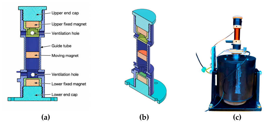
Figure 2.
Steady-state frequency response of the RMS output voltage VRMS(f) under harmonic excitation.
Figure 2.
Steady-state frequency response of the RMS output voltage VRMS(f) under harmonic excitation.
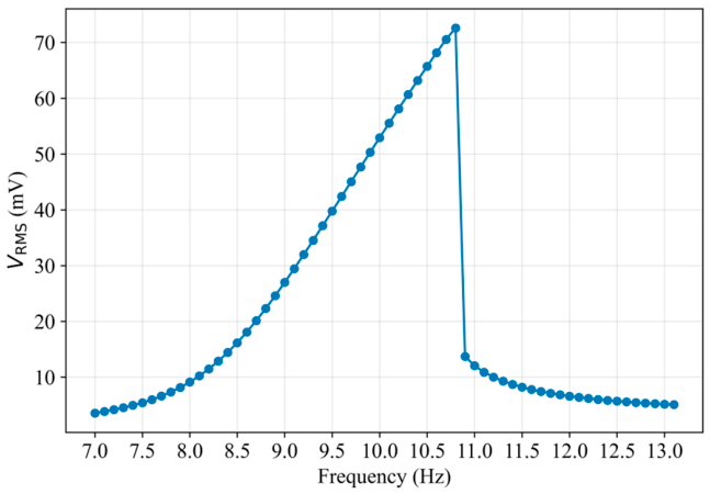
Figure 3.
Dynamic response of the energy harvester under steady-state excitation at the resonant frequency fr: (a) time history of the induced EMF; (b) phase portrait of the mechanical response z – ; (c) amplitude spectrum of the induced EMF.
Figure 3.
Dynamic response of the energy harvester under steady-state excitation at the resonant frequency fr: (a) time history of the induced EMF; (b) phase portrait of the mechanical response z – ; (c) amplitude spectrum of the induced EMF.
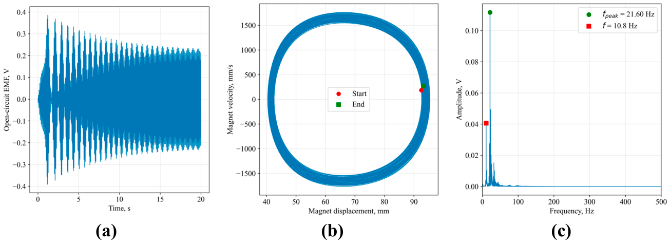
Figure 4.
Response surface of average output power as a function of excitation frequency and base acceleration amplitude: (a) heat map of power distribution; (b) 3D representation.
Figure 4.
Response surface of average output power as a function of excitation frequency and base acceleration amplitude: (a) heat map of power distribution; (b) 3D representation.
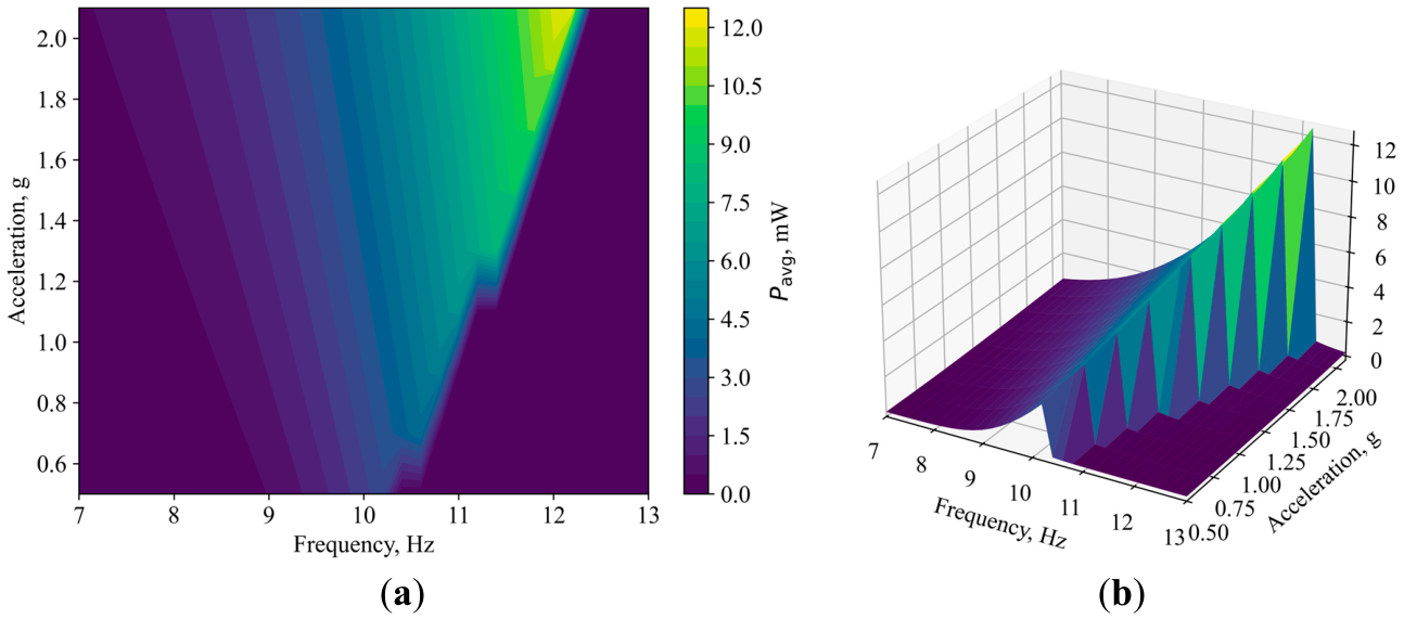
Figure 5.
Minimum average power in the vicinity of each operating point, expressed as a percentage of the overall maximum, given frequency deviations of ±0.2 Hz and base acceleration amplitude deviations of ±0.2 g.
Figure 5.
Minimum average power in the vicinity of each operating point, expressed as a percentage of the overall maximum, given frequency deviations of ±0.2 Hz and base acceleration amplitude deviations of ±0.2 g.
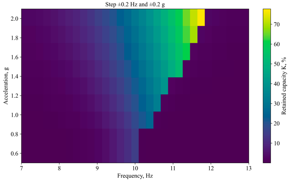
Figure 6.
Local relative power variation of the average output power for frequency deviations of ±0.2 Hz and base acceleration amplitude deviations of ±0.2 g.
Figure 6.
Local relative power variation of the average output power for frequency deviations of ±0.2 Hz and base acceleration amplitude deviations of ±0.2 g.
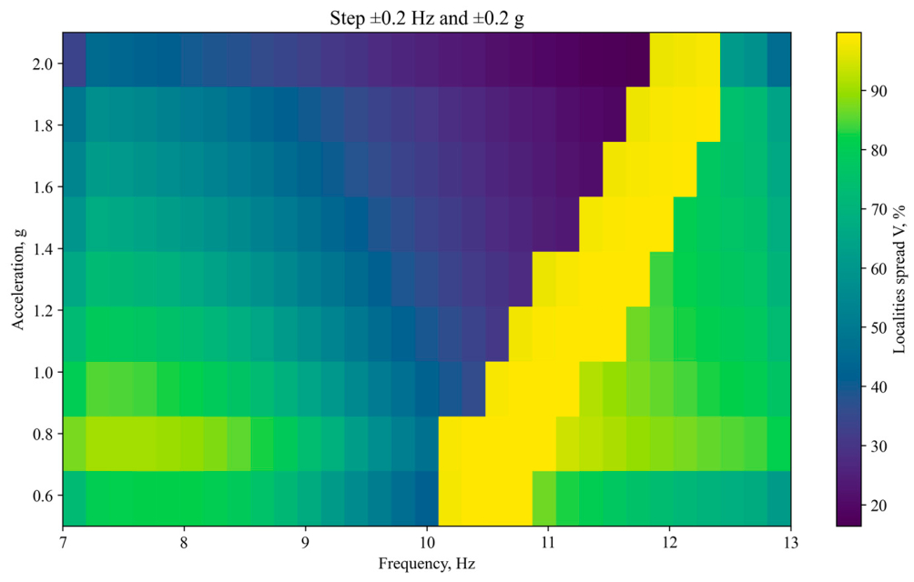

Table 1.
Key parameters of the energy harvester model.
| Parameter | Designation | Value |
|---|---|---|
| Mass of the moving element | m | 42.0 g |
| Residual magnetic induction | Br | 1.11 T |
| Magnet radius | r | 9.75 mm |
| Magnet height | hm | 10 mm |
| Coil resistance | Rc | 1 Ω |
| Coil inductance | Lc | 0.033 mH |
| Load resistance | RL | 1 Ω |
Table 2.
Vibration excitation parameters.
| Parameter | Designation | Value or range |
|---|---|---|
| Excitation frequency range | fmin − fmax | 7-13 Hz |
| Frequency step size | Δf | 0.2 Hz |
| Base acceleration amplitude | Ab | 0.5-2.1 g |
| Averaging time window | Tavg | 40 s |
Table 3.
Retained power fraction and local relative power variation for various limits of excitation parameter deviations.
Table 3.
Retained power fraction and local relative power variation for various limits of excitation parameter deviations.
| Maximum frequency deviation, Hz | Maximum acceleration deviation, g | Maximum retained power fraction Kglob,% | Local relative power variation Dloc, % |
|---|---|---|---|
| ±0.2 | ±0.2 | 77.73 | 16.46 |
| ±0.4 | ±0.4 | 57.58 | 33.24 |
| ±0.6 | ±0.6 | 39.71 | 50.15 |
| ±0.8 | ±0.8 | 24.58 | 66.48 |
Disclaimer/Publisher’s Note: The statements, opinions and data contained in all publications are solely those of the individual author(s) and contributor(s) and not of MDPI and/or the editor(s). MDPI and/or the editor(s) disclaim responsibility for any injury to people or property resulting from any ideas, methods, instructions or products referred to in the content. |
© 2026 by the authors. Licensee MDPI, Basel, Switzerland. This article is an open access article distributed under the terms and conditions of the Creative Commons Attribution (CC BY) license (http://creativecommons.org/licenses/by/4.0/).
Copyright: This open access article is published under a Creative Commons CC BY 4.0 license, which permit the free download, distribution, and reuse, provided that the author and preprint are cited in any reuse.