

Submitted:
08 October 2026
Posted:
09 October 2026
You are already at the latest version
Abstract
The goal of this study is to model the rate of change between spring and winter in groundwater quality for irrigation in coastal wells in the municipality of Guasave, Sinaloa, Mexico. In 58 well-water samples (29 sampled in spring and 29 in winter), the following parameters were measured: pH, electrical conductivity (E.C.), total dissolved solids, temperature, salinity, static water level, Na+, Ca2+, Mg2+, K+, Cl–, SO42–, CO32–, and HCO3–. The original sodium adsorption ratio (SARor), corrected (SARco), and adjusted (SARad) were calculated. For spring and winter and using Pearson and Spearman (Sr) coefficients, ordinary and repeated measures correlations were calculated. To identify differences between seasons, paired tests and Piper diagrams were used. The rate of quality change was modeled using multiple non-linear regressions. All models were rigorously validated. For the quality change rate, three predictive quadratic polynomial models were obtained. These three models presented the following significant values for Sr: 0.653 (E.C. vs. SARor), 0.575 (E.C. vs. SARco), and 0.470 (E.C. vs. SARad). Observed and predicted quality were numerically classified based on E.C. vs. SARor, SARco, and SARad. The information from these models can be applied to prevent soil contamination caused by irrigation with saline and sodic water, potentially boosting agricultural yields in ‘‘the agricultural heart of Mexico.’’
Keywords:
the agricultural heart of Mexico
; observed quality
; predicted quality
; sodium adsorption ratio
1. Introduction
Globally, groundwater is one of the most important freshwater resources [1]. Worldwide, approximately 20% of groundwater is used for agricultural irrigation [2,3]. As this water resource is essential, reliable, and constant [4], it supports the economic sector of any region [5]. In arid and semi-arid regions, the study of groundwater takes on greater importance due to its vulnerability [6,7]. This vulnerability is essentially due to the rate of change of physicochemical variables [8,9], which is accentuated when:
- a)
- b)
- The cumulative precipitation of summer (July–September) is approximately three-quarters of the total annual accumulation [11].
- c)
Groundwater inefficiency depends on multiple phenomena, such as recharge and dilution [4,7,14,15,16], salt dissolution and leaching [15,17], water–rock interaction [15,18], evaporation [19], and the rise and fall of the static water level (s.l.) [4,14]. According to [20,21], s.l. variation is highly related to extreme summer seasonal recharge [12] and is one of the factors most closely associated with variation in quality [9]. Irrigation water quality is evaluated, in accordance with [22,23], based on two parameters; electrical conductivity (E.C.) and sodicity. Multiple proposals have been developed to evaluate sodicity, three of which stand out: original sodium adsorption ratio (SARor), corrected (SARco), and adjusted sodium adsorption rate (SARad) [5,7,24]. According to [24,25], these three formulations require the cations Na+, Ca2+ and Mg2+ for their calculation; however, only two of them account for anion contamination; CO32– (SARco) and HCO3– (SARco and SARad).
In Mexico, multiple efforts have also been made to evaluate groundwater quality for irrigation for the spring and winter seasons [24,26]. These two sampling seasons are essential for understanding, in the context of extreme summer precipitation, for example, the dissolution and leaching of salts derived from agrochemicals [2,11,13,15]. The semi-arid municipality of Guasave is located in the northern part of the state of Sinaloa [27,28]. Due to its high agricultural productivity, this municipality is also known as ‘‘the agricultural heart of Mexico’’ [29]. Although [19] evaluated irrigation water quality (E.C. vs. SARor) for coastal wells in Guasave, predictive models of the rate of quality change between spring and winter are still lacking.
In this study, two groundwater sampling campaigns were conducted for the coastal portion of the Guasave municipality: spring (June 2025) and winter (February 2026). In each campaign, 29 irrigation wells were sampled. For each sample, the following variables were measured: pH, E.C., total dissolved solids (TDS), temperature (Temp), salinity (Sal), s.l., Na+, Ca2+, Mg2+, K+, Cl–, SO42–, CO32–, and HCO3–. SARor, SARco, and SARad were calculated. For all variables, two ordinary and one repeated-measure [30] Pearson (Pr) and Spearman (Sr) correlation were applied. For spring and winter, a paired test [31] was applied and a Piper diagram [23] was constructed. To model quality for spring and winter, as well as the rate of quality change between the two seasons, multiple linear (MLR) and non-linear (MNR) regressions were applied, prioritizing efficiency and ease of application [32]. Observed and predicted quality were numerically classified using the nomogram from [22] and based on E.C. vs. each of SARor, SARco, and SARad. To validate MLR and MNR, six and seven tests were applied, respectively.
The goal of this study is to model the rate of change between spring and winter of groundwater quality for irrigation in coastal wells in the municipality of Guasave, Sinaloa, Mexico.
The models in this study are easily to apply and can contribute to developing an efficient and effective method for preventing soil contamination [33] resulting from irrigation with saline and sodic groundwater. Preventing soil contamination can also foster optimal agricultural yields [18], helping to ensure food sovereignty and the socioeconomic development of one of the municipalities with the highest agricultural productivity in Mexico.
2. Materials and Methods
2.1. Study Area
2.1.1. Irrigated Agriculture, Geology, and Climatology
This study was conducted in the municipality of Guasave, which is considered “the agricultural heart of Mexico,” largely because approximately 181,542 hectares are irrigated; in other words, its economy relies to a large extent on activities associated with irrigated agriculture [29,34]. The crops primarily grown in this municipality are corn, potatoes, beans, green chili peppers, tomatoes, sorghum, and chickpeas [34].
The municipality of Guasave is composed of clastic sediments resting upon irregular igneous, sedimentary, and metamorphic rocks [19]. The deltaic plain is composed of sandy, silty, and clayey sediments, which originated during four epochs; the Oligocene, Miocene, Pliocene, and Pleistocene [35].
In the state of Sinaloa and for the year 2025, an average annual accumulated precipitation of 889.10 mm year⁻¹ was recorded, with the period June–October (the summer season) accounting for 97.64% of this precipitation [36]. The El Playón weather station (located approximately 47 km south of the city of Guasave) recorded an average annual accumulated precipitation of 463.03 mm year⁻¹ for the 1969–2018 period [28].
2.2. Location of the Study Area and Samples
This study focused on the coastal portion of the municipality of Guasave (Figure 1).
A water sample was randomly collected from each of 29 irrigation wells (Figure 1). Samples were collected from the same 29 wells during two seasons; spring (June 9–11, 2025) and winter (February 5–6, 2026), for a total of 58 samples.
2.3. Sample Storage
All samples were stored in 250 mL amber glass bottles at 4–10 °C [37]. Following measurement of s.l., to ensure the homogeneity of ionic concentration, each sample was collected after a minimum of three minutes of pumping. For metal measurement, each sample was acidified with 2.5 mL of 64.7% concentrated nitric acid [38].
2.4. Measurement and Calculation of Physicochemical Variables
Eight variables were measured in situ for each sample: TDS, Temp, pH, E.C., s.l., Na+, Sal, and Ca2+. In the laboratory, six additional variables were measured: Mg2+, K+, Cl−, SO42–, CO32– and HCO3–.
2.5. Normality, Ordinary Correlation, Repeated Measures Correlation, and Correlation Hypothesis Testing for Physicochemical Variables
Prior to calculating correlations between physicochemical variables, a Shapiro–Wilk normality test was applied [31].
Pr was applied to the series that exhibited normality, while Sr was applied to those that did not. Pr and Sr were applied in three instances: a) ordinary correlation for spring, b) ordinary correlation for winter, and c) repeated measures correlation for spring and winter [30], which evaluated the seasonal influence of summer. The values involved in this last correlation were obtained through the following subtraction: values that were applied in repeated measures correlation = winter values – spring values.
Through hypothesis testing, significant correlations were identified that met the criteria of either Pr ≥ ?Pearson’s critical correlation (Pcr)? or Sr ≥ ?Spearman’s critical correlation (Scr)? [42]. The Pcr and Scr coefficients considered in this study were 1) for n = 23 (Pcr = 0.413 and Scr = 0.418) and 2) for n = 29 (Pcr = 0.367 and Scr = 0.370).
2.6. Paired Tests
Paired sample mean difference tests were applied [31]. If both series of values showed normality, the Student’s t-test was applied; if one or both series were non-normal, the Wilcoxon test was applied.
2.7. Hydrochemical Composition
To identify seasonal changes in the hydrochemical composition and characterization of the water, a Piper diagram was constructed for spring and for winter data. This diagram is one of the most widely used plots in the literature, as it is particularly useful for examining evolutions and ionic mixtures [23,43,44].
2.8. Observed Irrigation Water Quality Classification, and Prediction–Classification of Irrigation Water Quality
The Richards nomogram [22] was used to classify the observed (Figure 2a) and predicted qualities (Figure 2b). This classification evaluates quality using two parameters; E.C. and SAR [23,45].
Specifically for observed quality classification, an arbitrary numerical value was assigned to each, ranging from C1–S1 = 1 to C5–S5 = 25 (Figure 2a).
For the predicted quality, polynomial-type MLR models were used as the first option. When an MLR model failed to meet one of the validation criteria, a quadratic polynomial-type MNR model was used as the second option. For the MLR and MNR dependent variables, the observed numerical values for three water quality parameters were used; E.C. vs. SARor, E.C. vs. SARco, and E.C. vs. SARad. Prioritizing ease of application, it was decided to use four and six independent variables; pH, E.C., Temp, and s.l. for MLR and pH, E.C., TDS, Temp, Sal, and s.l. for MNR. Once the numerical values for predicted quality were obtained, they were also classified using equivalence intervals from C1–S1 = 0.01–1.00 to C5–S5 = 24.01–25.00 (Figure 2b). Quality was predicted for three conditions: a) spring, b) winter, and c) difference between winter and spring.
2.9. Salinity (Sal) Estimation Regressions
It was decided to provide predictive models for Sal, based on E.C. This is in the case where salt meters in the wells are dispensed with.
To predict Sal, simple linear regressions were first applied. When normality was not observed in the residuals of these linear regressions, simple non-linear regressions were used as a second option, through a quadratic polynomial. Since the observed and predicted salinity series did not exhibit normality, Sr was applied. For the predicted Sal models to be considered significant, the condition Sr ≥ ?Scr? had to be met (Scr = 0.418, n = 23).
2.10. Validation of Predictive Quality Models
2.10.1. Normality, Homoscedasticity, Homogeneity and Independence of Residuals, Minimal Multicollinearity and Performance Metrics
Four validation tests were applied to the MLR residuals: 1) Shapiro–Wilk normality [46], 2) homoscedasticity (Breusch–Pagan and White) [47,48], 3) homogeneity [49], and 4) independence (Durbin–Watson) [50], (Box–Pierce) [51], (Ljung–Box) [51], and (McLeod–Li) [52].
Furthermore, for the MLR, it was verified that all independent variables exhibited minimal multicollinearity—specifically, a low variance inflation factor (VIF < 3.0) [53,54].
Seven performance tests were applied to the MLR and MNR; Sr (fit), coefficient of determination (), root mean square error (RMSE), mean square error (MSE), Nash–Sutcliffe efficiency (NSE), percent bias (PBIAS), and mean error (ME). These tests are widely used to evaluate the performance of predictive models [55,56,57,58,59,60]. According to [42,61], the optimal performances are Sr ?Scr? (Scr = 0.418, n = 23), R2 , RMSE 0.000, MSE 0.000, 0.750 NSE 1.000, PBIAS 10.000, and ME 0.000.
2.11. Software, Equipment, and Statistical Significance
The following software programs were used in this study: Paleontological Statistics (PAST) version 5.3, Microsoft Office 365, XLSTAT Advanced version 2026.1.0, and CorelDRAW 2019 version 21.0.0.593.
The following equipment was also used: a Garmin Map 62s GPS, two Hanna Instruments photometers models HI83399–01 (for Mg2+, K+, and Cl−), and HI83325–01 (for SO42−), a Hanna Instruments potentiometer HI98130 (for E.C., pH, Temp, and TDS), three Horiba LAQUAtwin ion-selective meters (for Na+, Ca2+, and Sal), and a level probe and Truper tape measure. CO32− and HCO3− were measured via volumetry, in accordance with [62].
The significance level for all statistical analyses isα = 0.05.
3. Results
3.1. Spring
3.1.1. Spatial Variability of Physicochemical Parameters
As shown in Table 1, the maximum, minimum, and average values for the physicochemical parameters are 8.23, 6.90, and 7.59 (pH); 14,910.00 μS cm⁻¹, 560.00 μS cm⁻¹, and 2,193.45 μS cm⁻¹ (E.C.); 7.46 ppt, 0.27 ppt, and 1.09 ppt (TDS); 40.10 °C, 27.00 °C, and 30.03 °C (Temp); 8.20% NaCl, 0.30% NaCl, and 1.26% NaCl (Sal); 5.89 m, 1.98 m, and 3.42 m (s.l.); and 117.44 mEq L⁻¹, 2.26 mEq L⁻¹, and 23.54 mEq L⁻¹ (Na⁺). The further maximum, minimum and average values are 20.96 mEq L–1, 0.42 mEq L–1, and 6.31 mEq L–1 (Ca2+); 33.74 mEq L–1, 0.66 mEq L–1, and 3.03 mEq L–1 (Mg2+); 1.38 mEq L–1, 0.04 mEq L–1, and 0.15 mEq L–1 (K+); 22.99 mEq L–1, 0.42 mEq L–1 and 3.42 mEq L–1 (Cl–); 14.16 mEq L–1, 0.35 mEq L–1, and 4.39 mEq L–1 (SO42–); all values zero for CO32–; 13.33 mEq L–1, 6.66 mEq L–1, and 10.25 mEq L–1 (HCO3–); 31.25, 1.33, and 12.55 (SARor ); 74.11, 3.29, and 31.00 (SARco); and 37.53, 2.09, and 17.03 (SARad) (Table 1).
3.1.2. Observed Irrigation Water Quality Classification
Based on the E.C. vs. SARor results (Figure 3a), the following quality classifications were recorded: one well with C5–S3 (well 20), one well with C3–S5 (well 17), six wells with C4–S4 (wells 1, 6, 9–11, and 21), four wells with C3–S4 (wells 13, 18, 28, and 29), two wells with C3–S3 (wells 12 and 24), eight wells with C3–S2 (wells 5, 8, 14–16, 22, 23, and 25), four wells with C3–S1 (wells 4, 7, 19, and 27), and three wells with C2–S1 (wells 2, 3, and 26). Figure 3b (E.C. vs. SARco) shows the following quality classifications: one well with C5–S5 (well 20), six wells with C4–S5 (wells 1, 6, 9–11, and 21), six wells with C3–S5 (wells 13, 17, 18, 24, 28, and 29), eight wells with C3–S4 (wells 5, 8, 12, 14, 16, 22, 23, and 25), two wells with C3–S3 (wells 15 and 27), three wells with C3–S2 (wells 4, 7, and 19), two wells with C2–S2 (wells 2 and 3), and one well with C2–S1 (well 26). Figure 3c (E.C. vs. SARad) shows the following quality classifications: one well with C5–S4 (well 20), one well with C4–S5 (well 9), two wells with C3–S5 (wells 17 and 28), five wells with C4–S4 (wells 1, 6, 10, 11, and 21), five wells with C3–S4 (wells 12, 13, 18, 24, and 29), four wells with C3–S3 (wells 5, 22, 23, and 25), seven wells with C3–S2 (wells 7, 8, 14–16, 19, and 27), one well with C3–S1 (well 4), and three wells with C2–S1 (wells 2, 3, and 26).
3.2. Winter
3.2.1. Spatial Variability of Physicochemical Parameters
As shown in Table 2, the maximum, minimum, and average values for the parameters are 8.09, 6.64, and 7.18 (pH); 10,230.00 μS cm⁻¹, 600.00 μS cm⁻¹; and 1,849.31 μS cm⁻¹ (E.C.); 5.13 ppt, 0.31 ppt, and 0.93 ppt (TDS); 29.10 °C, 21.70 °C, and 26.71 °C (Temp); 8.30% NaCl, 0.40% NaCl, and 1.22% NaCl (Sal); 6.80 m, 1.29 m, and 2.30 m (s.l.); and 213.14 mEq L⁻¹, 9.57 mEq L⁻¹, and 38.08 mEq L⁻¹ (Na⁺). The maximum, minimum, and average values for the remaining parameters are 23.95 mEq L–1, 0.55 mEq L−1, and 6.72 mEq L−1 (Ca2+); 40.32 mEq L–1, 0.74 mEq L–1, and 5.00 mEq L–1 (Mg2+); 1.85 mEq L–1, 0.04 mEq L−1, and 0.19 mEq L–1 (K+); 119.88 mEq L–1, 0.04 mEq L−1, and 7.13 mEq L–1 (Cl–); 13.12 mEq L–1, 0.92 mEq L–1, and 3.66 mEq L–1 (SO42–); all values zero for CO32–; 51.74 mEq L−1, 7.45 mEq L–1, and 17.83 mEq L–1 (HCO3–); 52.07, 3.60, and 18.51 (SARor); 89.92, 3.99, and 34.06 (SARco); and 66.91, 6.24, and 24.62 (SARad) (Table 2).
3.2.2. Observed Irrigation Water Quality Classification
The quality classifications for E.C. vs. SARor (Figure 4a) are: one well with C5–S5 (well 20), four wells with C3–S5 (wells 9, 13, 18, and 28), four wells with C4–S4 (wells 1, 6, 21, and 29), four wells with C3–S4 (wells 5, 11, 12, and 24), seven wells with C3–S3 (wells 8, 10, 14, 22, 23, 25, and 27), seven wells with C3–S2 (wells 2–4, 7, 16, 17, and 19), one well with C3–S1 (well 26), and one well with C2–S1 (well 15). For E.C. vs. SARco (Figure 4b), the quality classifications are: one well with C5–S5 (well 20), four wells with C4–S5 (wells 1, 6, 21, and 29), nine wells with C3–S5 (wells 9–13, 17, 18, 24, and 28), seven wells with C3–S4 (wells 5, 8, 14, 16, 22, 23, and 25), one well with C3–S3 (well 27), five wells with C3–S2 (wells 2–4, 7, and 19), one well with C3–S1 (well 26), and one well with C2–S3 (well 15). Figure 4c (E.C. vs. SARad) shows the following quality classifications: one well with C5–S5 (well 20), three wells with C4–S5 (wells 6, 21, and 29), four wells with C3–S5 (wells 9, 13, 18, and 28), one well with C4–S4 (well 1), seven wells with C3–S4 (wells 5, 10–12, and 23–25), eight wells with C3–S3 (wells 2, 3, 8, 14, 16, 17, 22, and 27), four wells with C3–S2 (wells 4, 7, 19, and 26), and one well with C2–S2 (well 15).
3.3. Correlational Analysis Between Physicochemical Variables
3.3.1. Ordinary Correlation for Spring
As presented in Table 3, the following Sr values for E.C. were significant: 0.997 (TDS), 0.933 (Sal), –0.463 (s.l.), 0.859 (Na+), 0.426 (Ca2+), 0.544 (Mg2+), 0.775 (Cl–), 0.843 (SO42−), 0.619 (SARor), 0.695 (SARco), and 0.668 (SARad).
SARor showed the following significant correlations: Pr = 0.489 (pH), Sr = 0.619 (E.C.), Sr = 0.611 (TDS), Sr = 0.531 (Sal), Sr = 0.880 (Na+), Sr = 0.563 (SO42–), and Pr = 0.541 (HCO3−). SARco was significantly correlated with E.C. (Sr = 0.695), TDS (Sr = 0.687), Sal (Sr = 0.604), Na+ (Sr = 0.927), Cl– (Sr = 0.406), SO42– (Sr = 0.638), and HCO3– (Pr = 0.489). SARad was significantly correlated with pH (Pr = 0.452), E.C. (Sr = 0.668), TDS (Sr = 0.659), Sal (Sr = 0.576), Na+ (Sr = 0.909), Cl– (Sr = 0.398), SO42– (Sr = 0.610), and HCO3– (Pr = 0.545).
Temp and K+ showed no significant correlation with E.C., SARor, RASco, or SARad.
3.3.2. Ordinary Correlation for Winter
As shown in Table 4, the significant values of Sr and for E.C. are 0.999 (TDS), 0.992 (Sal), 0.738 (Na+), 0.482 (Mg2+), 0.906 (Cl–),0.635 (SO42–),0.377 (SARor), and 0.499 (SARco).
SARor showed the following significant correlations for Sr: 0.741 (pH), 0.377 (E.C.), 0.377 (TDS), 0.860 (Na+), –0.625 (Ca2+), and –0.389 (Mg2+). SARco showed the following significant correlations: Pr = 0.708 (pH), Sr = 0.499 (E.C.), Sr = 0.501 (TDS), Sr = 0.479 (Sal), Sr = 0.867 (Na+), Sr = −0.370 (Ca2+), Sr = 0.424 (Cl–), and Sr = 0.511 (SO42–). The significant correlations for Sr and for SARad are 0.707 (pH), 0.370 (TDS), 0.826 (Na+), −0.576 (Ca2+), and –0.447 (Mg2+).
Temp, s.l., K+, and HCO3– showed no significant correlations with E.C., SARor, SARco, or SARad.
3.3.3. Repeated Measures Correlation (Difference Between Winter and Spring)
Table 5 shows the following significant correlations with E.C.: TDS (0.977), Sal (0.563), and SO4²⁻ (0.773).
As seen in Table 5, the significant Sr correlations are 0.671 for SARor vs. Na+ and −0.393 for SARor vs. Mg2+, 0.524 for SARco vs. Mg2+ and 0.605 for SARco vs. HCO3–, and 0.623 for SARad vs. Na+ and −0.455 for SARad vs. Mg2+.
S.l., Temp, K+, and SO4²⁻ showed no significant correlation with E.C., SARor, SARco, or SARad.
3.4. Paired Tests
Of 17 physicochemical variables (Table 6), only four did not show significant changes in the means: Sal (p-value = 0.101), Ca2+ (p-value = 0.503), Cl– (p-value = 0.756), and CO32– (p-value = identical samples).
3.5. Hydrochemical Composition
3.5.1. Spring
As seen in Figure 5, out of 29 samples, 18 have a sodium-bicarbonate composition, 8 are sodium chloride-sulfate, 2 are magnesium-calcium-sulfate-chloride, and 1 is a magnesium-calcium-bicarbonate. All samples were associated with two cations: Na+ (26 samples) and Ca2+ (3 samples). Twenty-three associations with anions were observed: 19 with HCO3– and 4 with Cl–, while 6 samples showed no dominant anion.
3.5.2. Winter
As shown in the Piper diagram in Figure 6, 22 wells had sodium-bicarbonate water, 5 had sodium-chloride-sulfate water, and 2 had calcium-magnesium-bicarbonate water. Twenty-seven samples were associated with Na+, and two samples showed no dominant cations. There were 24 associations with HCO3– and two with Cl–. Three samples showed no dominant anion.
3.6. Quality Predictive Models
Nine models were obtained for quality prediction: four MLR models (Equations 6 and 8–10) and five MNR models (Equations 7 and 11–14).
3.6.1. Salinity (Sal) Estimation Regressions
To predict Sal content based on E.C., two simple non-linear regressions were obtained (Equations 15 and 16). For observed and predicted spring Sal (Equation 15), the p-values were p(normal) = 7.903, p(normal) = 6.496, and Sr = 0.905, respectively. For observed and predicted salinity in winter (Equation 16), the p-values were p(normal) = 4.583, p(normal) = 3.658, and Sr = 0.993, respectively.
3.7. Validation of Predictive Quality Models
3.7.1. Normality, Homoscedasticity, Homogeneity and Independence of Residuals, Minimal Multicollinearity and Performance Metrics
In the results shown in Table 7, the residuals exhibiting normality ranged from p(normal) = 0.063 [winter (E.C. vs. SARor)] to p(normal) = 0.274 [winter (E.C. vs. SARco)]. Two models were non-normal; p(normal) = 0.030 [winter (E.C. vs. SARad)] and p(normal) = 0.002 [winter–spring (E.C. vs. SARor)].
Homoscedasticity ranged from p-value = 0.079 [Breusch–Pagan test for spring (E.C. vs. SARor)] to p-value = 0.878 [Breusch–Pagan test for winter (E.C. vs. SARco)]. Only one series was heteroscedastic: p-value = 0.040 (Breusch–Pagan test for spring [E.C. vs. SARco]).
All series that exhibited normality and homoscedasticity also exhibited homogeneity; that is, the means of the residuals were 0.000.
Models with independence ranged from p(value) = 0.117 [Ljung–Box test for winter–spring (E.C. vs SARco)] to p(value) = 0.942 [Durbin–Watson test for spring (E.C. vs SARor)]. One series showed autocorrelation, with a p-value of 0.036 [McLeod–Li test and for winter–spring (E.C. vs. SARad)] (Table 7).
3.7.2. Minimal Multicollinearity
As shown in in Table 7, the minimal multicollinearity of the predictors ranged from VIF = 1.053 (for Temp) to VIF = 1.372 (for E.C.) across two models; [winter (E.C. vs. SARor) and spring (E.C. vs. SARad)]. One series showed severe multicollinearity; namely VIF = 25.412 (for E.C.) in [winter–spring (E.C. vs. SARco)].
3.7.3. Performance Metrics
As seen in Table 7 and Figure 7, the correlations ranged from Sr = 0.470 (R² = 0.221) for winter–spring (E.C. vs. SARad, Figure 7i) to Sr = 0.922 (R² = 0.851) for spring (E.C. vs. SARco, Figure 7b). Further performance metrics, the maximum and minimum values, respectively, were 2.033 (Figure 7a) and 0.804 (Figure 7b) for RMSE, 4.134 (Figure 7a) and 0.646 (Figure 7b) for MEC, 1.000 (Figure 7g and Figure 7i.991 (Figure 7d) for NSE, 4.628 (Figure 7b) and 2.672 (Figure 7a) for PBIAS, and 7.405 (Figure 7b) and 3.669 (Figure 7i) for ME.
4. Discussion
According to [63], normal and non-alkaline water values (6.50 < pH < 8.40) like those shown in Table 1 and Table 2 indicate good nutrient availability [24]. These values indicating the lack of alkalinity are also decisive for the occurrence of zero CO32– concentrations [63]. In general, the decreases in the values of E.C., TDS, Temp, Sal, and SO₄²⁻ (Table 2) can be attributed to the fact that summer precipitation, accounting for 72.96% of the total annual accumulation [11], tends to recharge the Sinaloa river aquifer [19,35]. This recharge dilutes the ionic concentration of the water [19] and decreases the depth of s.l. [35]. Table 2 presents, in general terms, an incremental effect on the average values of six ions (Na+, Ca2+, Mg2+, K+, Cl–, and HCO3–) and three indices (SARor, SARco, and SARad). This incremental effect can be attributed to heterogeneous hydrochemical responses such as mineral dissolution [24,64], soil salt leaching [65], cation exchange [65], and mixing with seawater [66].
In this study, 43 samples (73.13% of the total; Figure 3 and Figure 4) align with the results found by [23], as these authors also identified a high salinity hazard (C3 classification). Waters classified as C3 can only be used to irrigate alfalfa, wheat, oats, and barley [24], as these are salt-tolerant rather than salt-sensitive crops [67]. Based on Figure 4, to avoid water with a high sodification hazard (S4 classification) and thereby prevent a negative impact on soil structure [68] and undesirable crop development [69], it is suggested to use the water during winter, as this tends to lower SARor, SARco, and SARad values.
As shown in Table 3, the highest correlations for E.C. were obtained with s.l., Na+, Ca2+, Mg2+, and SO42–, and for SAR with Na+, Cl–, SO42–, and HCO3–. These correlations can be attributed to an increase in ionic concentration due to evaporative and minimal recharge effects [17,19].
According to [17], the highest correlations in Table 4 [(E.C. vs. Cl–) and (SAR vs. pH, Ca2+, and Mg2+)] can be attributed to the effects of soil leaching, cation exchange, and salt dissolution. According to [70], the significant correlations in Table 5 demonstrate high consistency in the quality of E.C. vs. SO42–, SARor vs Na+, and HCO3–, and SARad vs Na+, and HCO3–. The opposite is true for SARor and SARad, which exhibit high inconsistency with Mg²⁺ [70].
As shown in Table 6, only four parameters (Sal, Ca²⁺, Cl⁻, and CO₃²⁻) showed no significant change in their mean values [31], a result attributable to the fact that recharge from precipitation has little influence on the magnitude of these four parameters [17].
Figure 5 presents 18 sodium bicarbonate water compositions, that is, four fewer samples than in Figure 6. This difference is attributed to the fact that recharge generates Na+ dissolution and reconcentration [24]. The opposite is true for the sodium chloride sulfate composition; in other words, Figure 5 presents 8 samples, three more than Figure 6. This effect is attributed to two causes; a) the precipitation of less soluble ions during the low-flow period [24], and b) the mobilization and redistribution of Cl⁻ of agricultural [71] or marine [72] origin.
The MLR (Equations 6 and 8–10) efficiently predict water quality because, as shown in Table 7, they satisfy the conditions of normality, homoscedasticity (absence of heteroscedasticity), homogeneity, independence (absence of autocorrelation), and minimal multicollinearity, while demonstrating reliable performance [39,42,48,53]. As stated by [39,42], MNR (Equations 7 and 11–14) demonstrate reliable performance.
The Sal models (Equations 15 and 16) showed a good fit, as they met the condition Sr > ?Scr? [42].
The quality models (Equations 6–14) might not be highly efficient, as only a single year of measurement is considered, for both spring and winter. It is recommended to evaluate quality over multiple years to attempt to capture the potential occurrence of extreme variability in precipitation, temperature, and evaporation events in Sinaloa [73]. This extreme variability can destabilize [74] the results regarding observed vs. predicted quality, which are shown in Figure 7 of this study. Another limitation of the models is the complexity and uncertainty inherent in non-linearity [75], as well as the potential failure to select the best-performing function [76].
5. Conclusions
To classify and predict irrigation water quality in spring and winter and based on the relationship of E.C. vs. SARor, SARco, and SARad, 17 physicochemical parameters were measured in 29 well-water samples. The study was conducted in the coastal portion of the municipality of Guasave, Sinaloa, Mexico.
A non-alkaline pH results in good nutrient availability, which is a major factor in all CO3²⁻ measurements being zero. The decreases in E.C., TDS, Temp, Salinity, and SO₄²⁻ during winter are due to dilution and a reduction in the depth of s.l. The increases observed in winter for the parameters evaluating sodicity (Na+, Ca2+, Mg2+, HCO3–, SARor, SARco, and SARad) were due to mineral dissolution, leaching of soil salts, cation exchange, and mixing with seawater.
Approximately three-quarters of the total samples showed a high salinity hazard (C3 classification); in other words, the use of these waters is recommended only for irrigating alfalfa, wheat, oats, and barley. To avoid a high risk of sodification (S4 classification), it is suggested to use the water only in winter.
The decline in quality depends significantly on the evaporative effect, minimal recharge, soil leaching, cation exchange, and salt dissolution. High quality consistency is evident when four dependencies are present: 1) E.C. vs. SO42–, 2) SARor vs. Na+, 3) SARco vs. Mg2+ and HCO3−, and 4) SARad vs. Na+. Mg2+ is significant for the occurrence of two major quality inconsistencies related to sodicity (SARor and SARad).
The means for Sal, Ca2+, Cl–, and CO32– are not significantly sensitive to dilution from seasonal summer recharge.
91.34% of the total hydrochemical compositions were sodium bicarbonate and sodium chloride sulfate types; spring (18 and 8 compositions, respectively) and winter (22 and 5 compositions, respectively).
Nine predictive models (four MLR and five MNR) of the water quality of wells intended for irrigation are provided. Predicting the rate of change in quality (Equations 12–14) for spring and winter is a methodology that has not previously been applied for the state of Sinaloa. This methodology can encourage the development of early strategies for soil and crop protection against the impacts of irrigation with saline and sodic water.
All models are mathematically validated; however, their predictive capacity could diminish with the occurrence of possible extreme weather events.
This methodology can be applied to any region of the world, and can thus be used to help increase crop yields without compromising the structural stability of the soils.
Author Contributions
Conceptualization, O.L.C.; investigation, L.C.A., N.P.M.S., L.A.S.G., and R.E.P.G.; data analysis, O.L.C., M.N.C., and L.C.A.; writing—original draft preparation, O.L.C; data curation, R.E.P.G., and J.A.A.D.; writing—review and editing, M.N.C., and L.C.A.
Funding
This research received no external funding.
Data Availability Statement
Data is contained within the article.
Acknowledgments
The authors thank the Secretariat of Research and Postgraduate from the National Polytechnic Institute for financial support provided through research projects with the following registration numbers: 20250798, 20254812, 20260688, and 20261040.
Conflicts of Interest
The authors declare no conflicts of interest.
References
- Singh, S.; Mondal, N.C.; Kaur, R.S. Assessment of groundwater quality for drinking and irrigation purposes using water quality index and statistical analysis in Nalanda district, South Bihar, India. Sci. Rep. 2026, 4, 406. [Google Scholar] [CrossRef]
- Raheja, H.; Goel, A.; Pal, M. An evaluation of groundwater quality and its suitability for drinking and irrigation uses under the GIS framework. Water Pract. Technol. 2022, 17, 11. [Google Scholar] [CrossRef]
- Dimple; Kumar, M.H.; Kumar, S.P.; Yadav, K.K.; Ram, B.S.; Rajput, J. Groundwater quality parameters for irrigation utilization: A review. Indian J. Agric. Sci. 2022, 92, 7. [Google Scholar] [CrossRef]
- Kumar, S.S.; Sharma, A. Evaluation and prediction of groundwater quality for irrigation using regression and machine learning models. Water Qual. Res. J. 2025, 60, 1. [Google Scholar] [CrossRef]
- González, V.A.C.; Chong, T.; Arrocha, J.; Lloyd, J.; Olmos, J.; Vergara, F.; Denvers, M.; Jaén, J.; Jiménez, O.S.; García, N.F.J. Geochemical Characterization of Soil andWater in an Agricultural Area for the Sustainable Use of Natural Resources. Agriculture 2025, 15, 702. [Google Scholar] [CrossRef]
- Yazdi, S.H.; Robati, M.; Samani, S.; Hargalani, F.Z. Assessing the sustainability of groundwater quality for irrigation purposes using a fuzzy logic approach. Environ. Sustain. Ind. 2024, 22, 100342. [Google Scholar] [CrossRef]
- El Hassan, G.; Naser, R.S.M.; Mahdaly, R.; Darwesh, N.; El-Bakkali, M.; Belghyti, D. Assessment of irrigation groundwater quality in Souk El Arbaa, Morocco. Water Sci. 2025, 39, 1. [Google Scholar] [CrossRef]
- Ha, K.; Lee, E.; An, H.; Kim, S.; Park, C.; Kim, G.B.; Ko, K.S. Evaluation of Seasonal Groundwater Quality Changes Associated with Groundwater Pumping and Level Fluctuations in an Agricultural Area, Korea. Water 2021, 13, 51. [Google Scholar] [CrossRef]
- Guo, Z.; Fogg, G.E.; Chen, K.; Pauloo, R.; Zheng, C. Sustainability of regional groundwater quality in response to managed aquifer recharge. Water Resour. Res. 2023, 59, e2021WR031459. [Google Scholar] [CrossRef]
- Beisenova, R.; Orkeyeva, A.; Rakhmetova, A.; Rakhymzhan, Z.; Tazitdinova, R. Hydroclimatic Variability andWater Balance Instability in Semi-Arid Steppe Ecosystems Under ClimateWarming. Resources 2026, 15, 97. [Google Scholar] [CrossRef]
- Llanes, C.O. Predictive association between meteorological drought and climate indices in the state of Sinaloa, northwestern Mexico. Arab. J. Geosci. 2023, 16, 79. [Google Scholar] [CrossRef]
- Thomas, B.F.; Behrangi, A.; Famiglietti, J.S. Precipitation Intensity Effects on Groundwater Recharge in the Southwestern United States. Water 2016, 8, 90. [Google Scholar] [CrossRef]
- Gebrehiwet, M.; Tafesse, N.T.; Habtu, S.; Alemaw, B.F.; Laletsang, K.; Lasarwe, R. The Contribution of Groundwater to the Salinization of Reservoir-Based Irrigation Systems. Agronomy;Agronomy 2021, 11, 512. [Google Scholar] [CrossRef]
- Sun, M.; Zhang, J.; Qin, J.; Li, H.; Zhang, L. Alternative to Groundwater Drip Irrigation for Tomatoes in Cold and Arid Regions of North China by Rainwater Harvesting from Greenhouse Film. Agronomy 2026, 16, 132. [Google Scholar] [CrossRef]
- Missaoui, R.; Gentilucci, M.; Hamed, Y.; Hadji, R.; Bouri, S.; Pambianchi, G. Irrigation-Driven Groundwater Recharge and Quality Degradation in Semi-Arid Regions: Hydrochemical, GIS-Based, and Explainable Machine Learning Assessment in Central Tunisia. Appl. Sci. 2026, 16, 7014. [Google Scholar] [CrossRef]
- Moges, S.S.; Dinka, M.O. Evaluation of shallow groundwater suitability for irrigation purposes: A case study from Doornfontein area, South Africa Evaluation of shallow groundwater suitability for irrigation purposes: A case study from Doornfontein area, South Africa. J. Water Land Dev. 2023, 58. Available online: https://www.jwld.pl/files/2023-03-JWLD-21.pdf. [CrossRef]
- Amouyal, A.; Reichmann, O.; Litaor, M.I. Modeling salinity and sodicity risks under long-term irrigation with medium salinity water: kinnerest catchment as a case study. Agric. Water Manag. 2026, 326, 110245. [Google Scholar] [CrossRef]
- Tejashvini, A.; Thimmappa, C.S.; Mudalagiriyappa, D.C.H.; Ramamurthy, V. Assessment of irrigation water quality for groundwater in Semi-Arid Region, Bangalore, Karnataka. Water Sci. 2024, 38, 1. [Google Scholar] [CrossRef]
- Peinado, G.H.J.; Green, R.C.R.; Herrera, B.J.; Escolero, F.O.A.; Delgado, R.O.; Belmonte, J.S.I.; Ladrón, G.M.A. Calidad y aptitud de uso agrícola y doméstico del agua del acuífero del río Sinaloa, porción costera. Hidrobiológica 2011, 21(1), 63–76. Available online: https://www.scielo.org.mx/scielo.php?script=sci_arttext&pid=S0188-88972011000100006.
- Duc, H.D.; Dan, N.H.; Binh, N.C.; Oanh, N.T. Evaluation of Groundwater Quality and Effects of Exploitation on Static Groundwater Levels in Dong Thap Province, Viet Nam. Water Resour. 2025, 52, 5. [Google Scholar] [CrossRef]
- Gbadebo, A.M.; Egbedara, T.A.; Gbadebo, O.O.; Dimowo, B.O. Geochemical evaluation of groundwater quality in Yewa for drinking and irrigation purposes. Water Sci. 2026, 40, 54. [Google Scholar] [CrossRef]
- Richards, L.A. Diagnosis and Improvement of Saline and Alkali Soils. In LWW; Washington, D.C. USA, 1954; Volume 78, Available online: https://www.ovid.com/jnls/soilsci/abstract/00010694-195408000-00012~diagnosis-and-improvement-of-saline-and-alkali-soils?redirectionsource=fulltextview.
- Kherouf, M.; Maoui, A.; Boumaaza, M.; Belaadi, A.; Abdullah, M.; Mukalazi, H.; Ghernaout, D.; Al-Khawlani, A. Evaluation and Prediction of Seybouse River Water Quality Using Response Surface Methodology and Machine Learning. Sci. Rep. 2026, 1, 1. [Google Scholar] [CrossRef] [PubMed]
- Can, C.A.; Ortega, E.H.M.; Sánchez, B.E.I.; Cruz, C.E. Calidad del agua para riego en la Sierra Norte de Puebla, México. Tecnol. Cienc. Agua 2014, 5, 5. Available online: https://www.scielo.org.mx/scielo.php?pid=S2007-24222014000500005&script=sci_arttext.
- Lesch, S.M.; Suarez, D. L. Technical note: a short note on calculating the adjusted SAR index. Trans. ASABE 2009, 52(2), 493–496. [Google Scholar] [CrossRef]
- Mancilla, V.O.R.; Villafaña, C.F.; Can, C.Á.; Guevara, G.R.D.; Olguín, L.J.L.; Cruz, C.E.; Luna, F.J.A.; Avelar, R.J.U. Quality of Surface and Groundwater in the Sierra de Amula Region, Jalisco, Mexico. Agriculture 2025, 15, 278. [Google Scholar] [CrossRef]
- Franco, O.C.; García, P.F.; Plata, R.W.; Montoya, R.J.M.; Vergara, S.M.A. Observaciones y análisis de parámetros hidromorfológicos de la playa Las Glorias, México. Tecnol. Cienc. Agua 2019, 10, 2. [Google Scholar] [CrossRef]
- González, G.G.E.; Llanes, C.O.; Norzagaray, C.M.; García, S.L.A.; Parra, G.R.E.; Ávila, D.J.A.; Arciniega, G.M.A. Variability, Prediction, and Simulation of Rainfall Erosivity Risk in the State of Sinaloa, Northwest Mexico. Atmosphere 2026, 17, 80. [Google Scholar] [CrossRef]
- Ahumada, C.R.; González, M.L.C.; Martínez, A.I.G.; Rodríguez, G.H.B. Exploring climate change perceptions, climate trends and the level of knowledge on the subject in farmers from Guasave, Mexico. Geo J. 2023, 88, 6453–6465. [Google Scholar] [CrossRef]
- Bakdash, J.S.; Marusich, L.R. Repeated Measures Correlation. Front. Psychol. 2017, 8, 456. [Google Scholar] [CrossRef] [PubMed]
- Alciaturi, G. Seasonal and spatial effects of land use and land cover on stream water quality in a South American rice producing region. Discov. Water 2026, 6, 40. [Google Scholar] [CrossRef]
- Molla, K.S.; Zewdu, W.B.; Kacprzak, G.; Bewket, D.M.; Dires, S.S. Machine learning models for predicting soil shear strength using geotechnical parameters and explainable artificial intelligence. Sci. Rep. 2026. [Google Scholar] [CrossRef]
- Ataklti, B.; Tesema, W.F.; Abadi, B.B. Integrated evaluation of groundwater irrigation suitability using hydrochemical indices and irrigation water quality index (IWQI) in Aksum, Tigray, Ethiopia. Sci. Rep. 2026, 16, 11072. [Google Scholar] [CrossRef] [PubMed]
- Ahumada, C.R.; Veázquez, A.G.; Ahumada, C.B. Adaptación del sector agrícola ante el cambio climático: propuesta de medidas a escala espacial fina en Guasave, Sinaloa, México. Acta Univ. 2018, 28(1), 46–56. [Google Scholar] [CrossRef]
- Norzagaray, C.M.; Muñoz, S.P.; Le Bail, M. Hydrological Stress and Climate Change Impact in Arid Regions with Agricultural Valleys in Northern Mexico. Adv. Environ. Monit. Assessment. IntechOpen 2019, 1, 3–19. [Google Scholar] [CrossRef]
- Comisión Nacional del agua (CONAGUA). Precipitación por entidad federativa para el año 2025. Available online: https://smn.conagua.gob.mx/tools/DATA/Climatología/Pronóstico%20climático/Temperatura%20y%20Lluvia/PREC/2025.pdf (accessed on 12 June 2026).
- Norma oficial mexicana NOM-014-SSA1-1993; Procedimientos sanitarios para el muestreo de agua para uso y consumo humano en sistemas de abastecimiento de agua públicos y privados (8p.). Secretaría de Salud: México, D.F. Available online: https://www.comapareynosa.gob.mx/resources/other/reglamentos/NOM-014-SSA1-1993.pdf (accessed on 05 June 2026).
- Norma mexicana NMX-AA-051-SCFI-2016. Análisis de agua.- medición de metals por absorción atómica en aguas naturales, potables, residuals y residuals tratadas-método de prueba. 39p. Available online: http://www.economia-nmx.gob.mx/normas/nmx/2010/nmx-aa-051-scfi-2016.pdf (accessed on 09 June 2026).
- Hussein, E.E.; Derdour, A.; Zerouali, B.; Almaliki, A.; Wong, Y.J.; Ballesta; de los Santos, M.; Minh, N.P.; Hashim, M.A.; Elbeltagi, A. Groundwater Quality Assessment and IrrigationWater Quality Index Prediction Using Machine Learning Algorithms. Water 2024, 16, 264. [Google Scholar] [CrossRef]
- Bower, C.A.; Ogata, G.; Tucker, J.M. Sodium Hazard of Irrigation Waters as Influenced by Leaching Fraction and by Precipitation or Solution of Calcium Carbonate. Soil Sci. 1968, 106(1), 29–34. Available online: https://www.ovid.com/jnls/soilsci/abstract/00010694-196807000-00005~sodium-hazard-of-irrigation-waters-as-influenced-by-leaching?redirectionsource=fulltextview. [CrossRef]
- Langelier, W.F. The Analytical Control of Anticorrosion Water Treatment. J. Am. Water Work. Assoc. 1936, 28, 1500–1521. Available online: https://cpoclass.com/wp-content/uploads/2021/08/Journal-of-the-American-Water-Works-Association-1936-10_-Vol-28-Iss-10.pdf. [CrossRef]
- Oxford Cambridge and RSA (OCR). Statistical Problem Solving: Formulae and Statistical Tables (ST1). Manual. Available online: https://www.ocr.org.uk/Images/727354-question-paper-statistical-problem-solving-formulae-and-statistical-tables.pdf (accessed on 15 August 2026).
- Musa, O.K.; Kudamnya, E.A.; Omali, A.O.; Akuh, T.I. Physico-chemical characteristics of Surface and groundwater in Obajana and its environs in Kogi State, Central Nigeria. Afr. J. Environ. Sci. Technol. 2014, 8, 9. [Google Scholar] [CrossRef]
- Malagón, J.P.; Piña, A.; Argüello, S.; Leonardo, D.D. Análisis hidrogeoquímico-multivariado del agua subterránea del sistema acuífero del Valle Medio del Magdalena, Colombia: Estudio a escala regional. Bol. Soc. Geol. Mex. 2021, 73(3), 00020. [Google Scholar] [CrossRef]
- Camacho, B.A.; Ortega, E.H.M.; Sánchez, B.E.I.; Can, C.A. Indicadores de calidad físico-química de las aguas residuales del estado de Oaxaca, México. Terra Latinoam. 2020, número especial: 38–2, 361–375. [Google Scholar] [CrossRef]
- Fasahat, P.; Solhdar, K.R.J.; Piepho, H.P. Using diagnostic residual plots to validate statistical assumptions in multi-environment sugar beet trials. Discov. Agric. 2026, 4, 175. [Google Scholar] [CrossRef]
- Hossain, M.I.; Jahan, E.; Ara, B.M.E. Climatic and non-climatic impacts on fish production in Bangladesh by using autoregressive distributed lag model. Discov. Environ. 2026, 4, 195. [Google Scholar] [CrossRef]
- Johannes, H.N.; Romeo, A.A.; Pangeiko, N.J. Interannual climate variability and hydropower generation sensitivity at Ruacana station with implications for energy security in Namibia. Discov. Sustain. 2026, 7, 646. [Google Scholar] [CrossRef]
- Carrasquilla, B.A.; Chacón, R.A.; Núñez, M.K.; Gómez, E.O.; Valverde, J.; Guerrero, B.M. Regresión Lineal Simple y Múltiple: Aplicación en la Predicción de Variables Naturales Relacionadas con el Crecimiento Microalgal. Tecnol. Marcha 2016, Encuentro de Investigación y Extensión, 33–45. Available online: https://www.scielo.sa.cr/scielo.php?script=sci_arttext&pid=S0379-39822016000900033.
- Almojel, S. Wheat yield dynamics in Saudi Arabia: evidence on short and long-run determinants. J. Saudi Soc. Agric. Sci. 2026, 25, 62. [Google Scholar] [CrossRef]
- Horváth, L.; Hušková, M.; Rice, G. Test of independence for functional data. J. Multivar. Anal. 2013, 117, 100–119. [Google Scholar] [CrossRef]
- Grivas. An Automatic Portmanteau Test For Nonlinear Dependence. Econom. Stat. 2025, 35, 71–83. [Google Scholar] [CrossRef]
- Khudari, M.; Hashimi, A.N.; Hamisham, H.N. Asymmetric impacts of global competitiveness and foreign direct investment on green total factor productivity in Oman. Discov. Sustain. 2026, 7, 602. [Google Scholar] [CrossRef]
- Kapetanakis, K.M.; Floros, C. Exploring the trade-offs between environmentally oriented policies and financial performance in U.S. banks: non-linear and heterogeneous effects. Oper. Res. 2026, 26, 67. [Google Scholar] [CrossRef]
- Liu, D.; Wang, K.; Bian, Y.; Wang, X.; Zhang, Y. Correlation analysis between the collapsibility of loess and physicomechanical indices in Longdong region and prediction of the collapsibility coefficient based on machine learning. Sci. Rep. 2026, 16, 15939. [Google Scholar] [CrossRef] [PubMed]
- Dhage, H.B.; Khedkar, N.K.; Naidu, M.J.; Salunkhe, S.; Cepova, L.; Nasr, E.A. Predictive modeling and experimental validation of mechanical–microstructural relationchips in 3D-printed Onyx–fibre composites. Sci. Rep. 2026, 16, 14715. [Google Scholar] [CrossRef] [PubMed]
- Bicák, D.; Brodsky, L. Efficiency of spatially multiscale machine learning models in addressing spatial non-stationarity and enhancing predictive accuracy. J. Geogr. Syst. 2026. [Google Scholar] [CrossRef]
- Gopika, S.V.; Shwetha, V.; Maddodi, B.S.; Kesiya, K.W. Machine learning-based predictive modelling and feature importance analysis of geomorphometric parameters in the Gangolli River Basin, Western Ghats, India. Discov. Appl. Sci. 2026, 8, 666. [Google Scholar] [CrossRef]
- Balacumaresan, H.; Imteaz, M.A.; Hossain, I.; Aziz, M.A.; Choudhury, T. Evaluation of Deep Learning and Physically Based Models for Urban Streamflow Estimation Under Historical and Future Climate Conditions. Water Resour. Manag. 2026, 40, 347. [Google Scholar] [CrossRef]
- Pankaj, D. Package “PerMat” (version 0.1.0): Performance metrics in predictive modeling in R. Available online: https://cran.r-project.org/web/packages/PerMat/PerMat.pdf (accessed on 01 June 2026).
- Kashavar, M.M.; Shahbazi, Y.; Amirkhiz, H.S.; Pedrammehr. Ensemble predictive structural health monitoring of space frame structures using deep learning models. Discov. Civ. Eng. 2026, 3, 192. [Google Scholar] [CrossRef]
- Norma oficial mexicana NOM-021-RECNAT-2000. Que establece las especificaciones de fertilidad, salinidad y clasificación de suelos. Estudios, muestreo y análisis. 73p. Available online: https://www.dof.gob.mx/nota_detalle.php?codigo=717582&fecha=31/12/2002#gsc.tab=0 (accessed on 21 June 2026).
- Can, C.A.; Ortega, E.H.M.; García, C.N.E.; Reyes, O.A.L.; González, H.V.A.; Flores, R.D. Origen y calidad del agua subterránea en la cuenca oriental de México. Tecnol. Cienc. Agua 2011, 29. Available online: https://www.scielo.org.mx/scielo.php?script=sci_arttext&pid=S0187-57792011000200189.
- Amihere, A.P.; Monney, I.; Okyere, D.C.; Adjei, K.A.; Appiah, A.E.K. Assessing the potential of managed aquifer recharge using rooftop rainwater harvesting with shallow wells in peri-urban communities in Kumasi, Ghana. Discov. Water 2025, 5, 52. [Google Scholar] [CrossRef]
- Dong, Y.; Shen, Z.; Li, J.; Sang, S.; Liu, C.; Sun, Z.; Gao, Y. Spatial-seasonal variability of hydrochemistry and lake water-groundwater interaction in the Poyang Lake Basin, China. Environ. Earth Sci. 2026, 85, 232. [Google Scholar] [CrossRef]
- Hu, C.; Yuan, X.; Wang, X. Impacts of geothermal exploitation on hydrochemical evolution in coastal granite fissure systems: evidence from Baoquan hot spring. Environ. Earth Sci. 2025, 84, 583. [Google Scholar] [CrossRef]
- González, P.E.; Ortega, E.H.M.; Yáñez, M.M.J.; Rodríguez, G.A. Diagnóstico de indicadores de calidad físico-química del agua en efluentes del río Atoyac. Tecnol. Cienc. Agua 2019, 10, 1. [Google Scholar] [CrossRef]
- Sattari, M.T.; Feizi, H.; Colak, M.S.; Ozturk, A.; Apaydin, H.; Ozturk, F. Estimation of sodium adsorption ratio in a river with kernel-based and decision-tree models. Environ. Monit. Assess. 2020, 192, 575. [Google Scholar] [CrossRef] [PubMed]
- Achite, M.; Katipoğlu, O.M.; Elshaboury, N.; Kartal, V.; Aktürk, G.; Ertugay, N. Modeling of irrigation water quality parameter (sodium adsorption ratio) using hybrid swarm intelligence-based neural networks in a semi-arid environment at SMBA dam, Algeria. Theor. Appl. Climatol. 2024, 155. [Google Scholar] [CrossRef]
- Kondo, M.; Nagashima, K.; Sato, Y. Weighted Repeated Measures Correlation Coefficient: A New Correlation Coefficient for Handling Missing Data With Repeated Measures. Stat. Med. 2025, 44, e70046. [Google Scholar] [CrossRef] [PubMed]
- Huepa, B.J.A.; Florez, Y.G.Y.; Hernandez, D. Causes and effects of contamination of water sources due to excessive use of agrochemicals and pesticides: bibliometric analysis. Water Policy 2024, 26, 11. [Google Scholar] [CrossRef]
- Costall, A.R.; Harris, B.D.; Teo, B.; Schaa, R.; Wagner, F.M.; Pigois, J.P. Groundwater Throughflow and Seawater Intrusion in High Quality Coastal Aquifers. Sci. Rep. 2020, 10, 9866. [Google Scholar] [CrossRef] [PubMed]
- Mora, F.Z.D.; Monjardin, A.S.A.; Rangel, P.J.G.; Rentería, G.S.A.; Sanhouse, G.A.J.; Bustos, T.Y. 92-year meteorological datasets from 50 meteorological stations in Sinaloa, Mexico with daily, monthly, and yearly resolutions. Data Brief. 2025, 62, 112041. [Google Scholar] [CrossRef] [PubMed]
- Riley, R.D.; Collins, G.S. Stability of clinical prediction models developed using statistical of machine learning methods. Biomed. J. 2023, 65, 8. [Google Scholar] [CrossRef] [PubMed]
- Nuttall, W.; Patelli, E.; Smith, E.; Wood, D.W.; Middleburgh, S. Perspectives on Engineering Uncertainty; Springer: Switzerland, 2025; pp. 1–101. [Google Scholar] [CrossRef]
- Dankers, F.J.W.M.; Traverso, A.; Wee, L.; Van Kuijk, S.M.J. Prediction Modeling Methodology in Fundamentals of Clinical Data Science; Springer, 2025; pp. 101–120. [Google Scholar] [CrossRef] [PubMed]
Figure 1.
Study area (coastal portion of the municipality of Guasave).
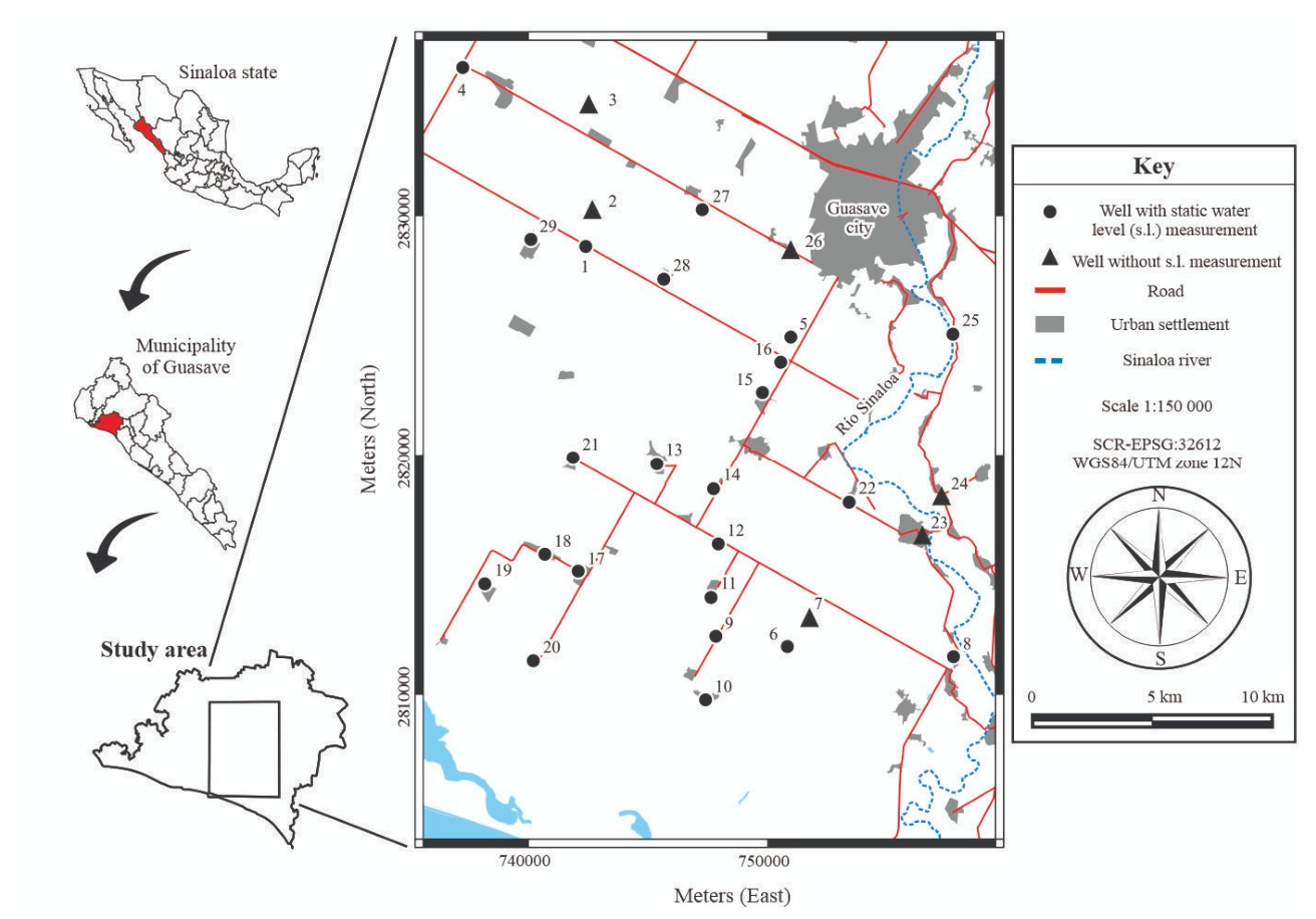
Figure 2.
Numerical intervals proposed for classifying irrigation water quality: a) observed and b) predicted.
Figure 2.
Numerical intervals proposed for classifying irrigation water quality: a) observed and b) predicted.
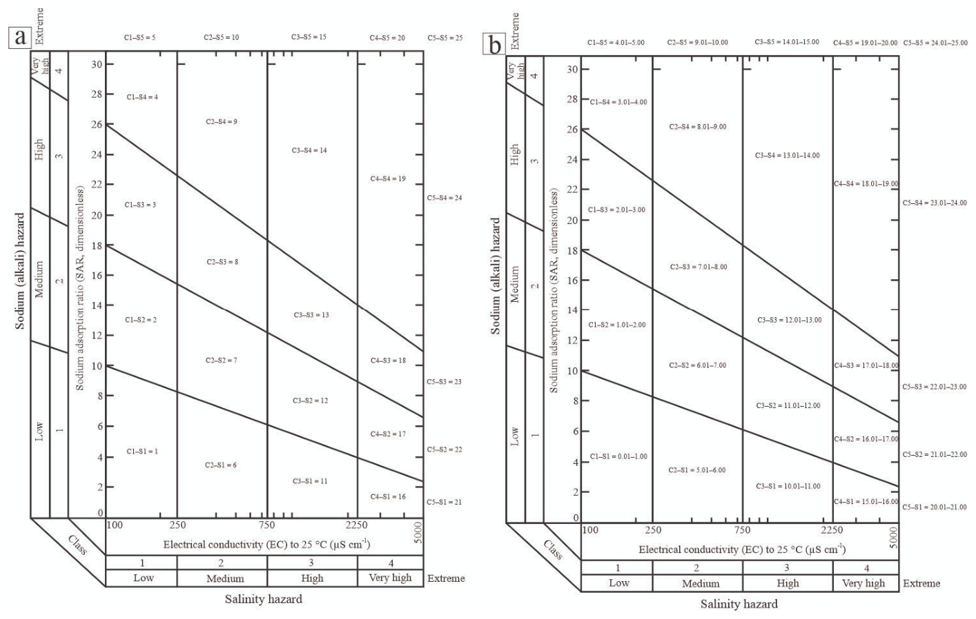
Figure 3.
Classification of observed irrigation water quality in spring, which evaluates electrical conductivity (E.C.) vs. sodium adsorption ratio (SAR): a) E.C. vs. original SAR (SARor), b) E.C. vs. corrected SAR (SARco), and c) E.C. vs. adjusted SAR (SARad). Wells with extreme E.C. and SAR values are not shown.
Figure 3.
Classification of observed irrigation water quality in spring, which evaluates electrical conductivity (E.C.) vs. sodium adsorption ratio (SAR): a) E.C. vs. original SAR (SARor), b) E.C. vs. corrected SAR (SARco), and c) E.C. vs. adjusted SAR (SARad). Wells with extreme E.C. and SAR values are not shown.
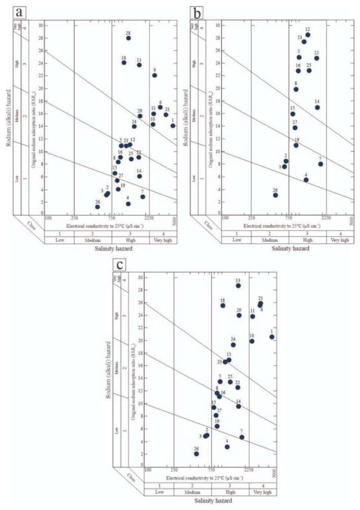
Figure 4.
Classification of observed irrigation water quality in winter, which evaluates electrical conductivity (E.C.) vs. sodium adsorption ratio (SAR): a) E.C. vs. original SAR (SARor), b) E.C. vs. corrected SAR (SARco), and c) E.C. vs. adjusted SAR (SARad). Wells with extreme E.C. and SAR values are not shown.
Figure 4.
Classification of observed irrigation water quality in winter, which evaluates electrical conductivity (E.C.) vs. sodium adsorption ratio (SAR): a) E.C. vs. original SAR (SARor), b) E.C. vs. corrected SAR (SARco), and c) E.C. vs. adjusted SAR (SARad). Wells with extreme E.C. and SAR values are not shown.
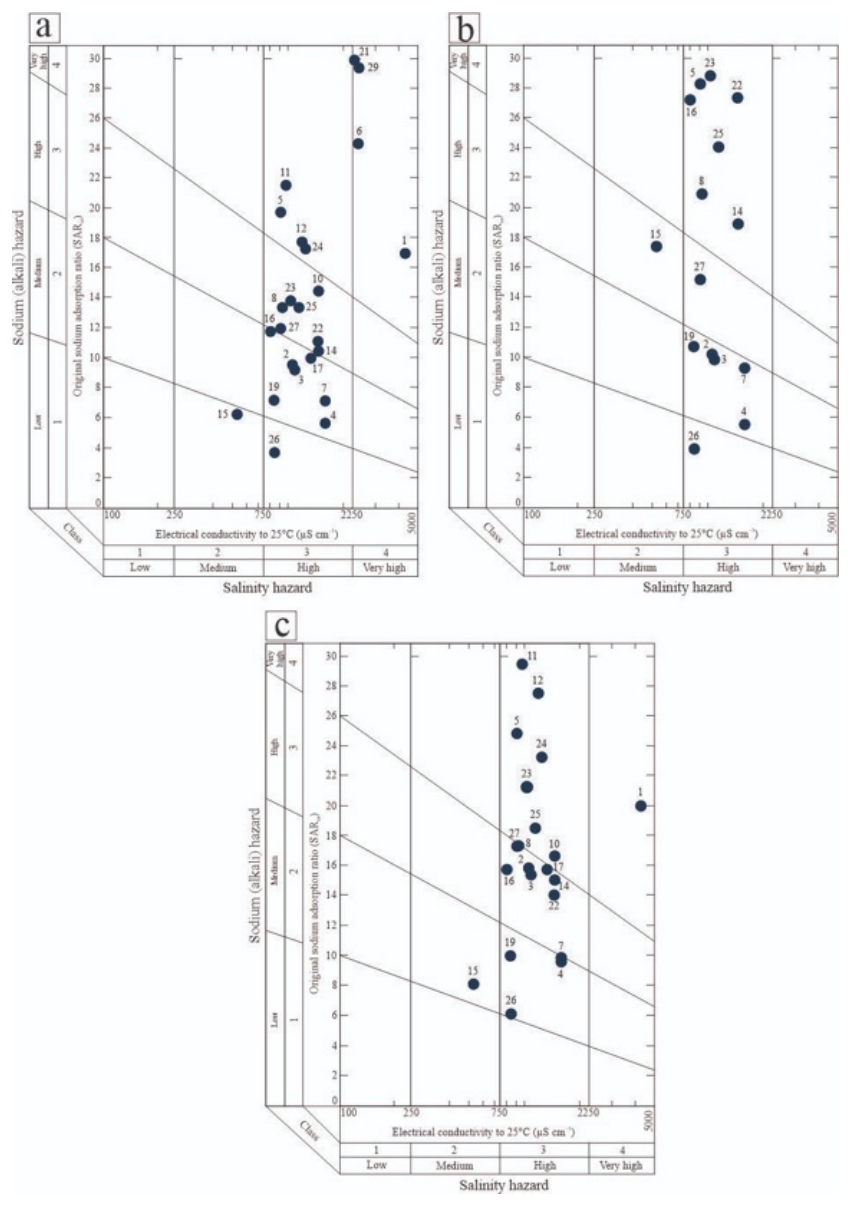
Figure 5.
Hydrochemical composition for spring shown as a Piper diagram.
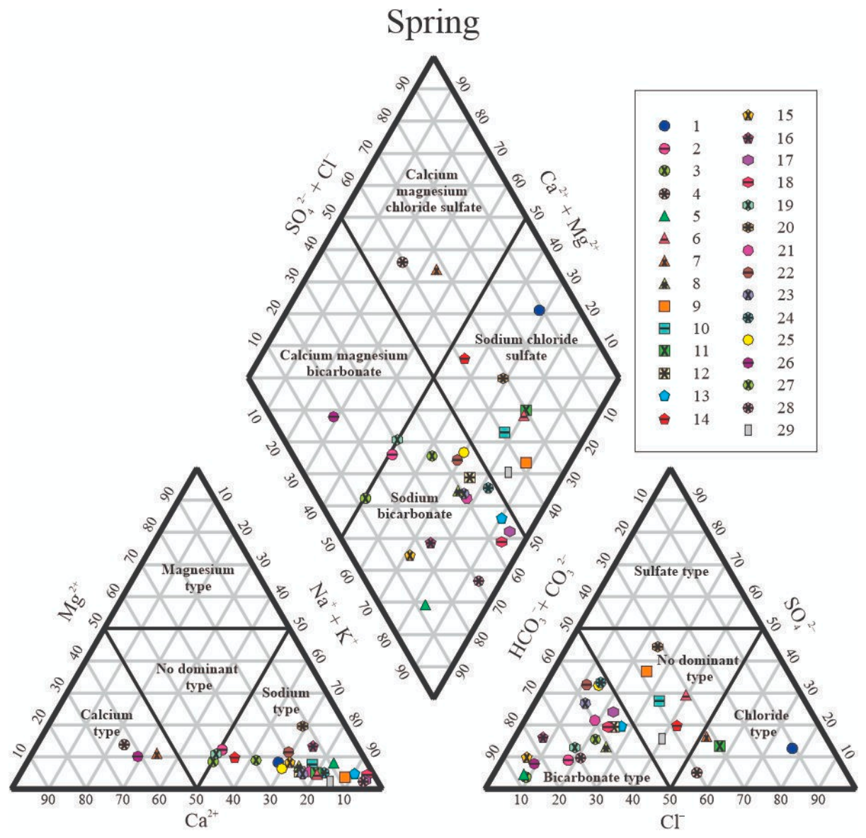
Figure 6.
Hydrochemical composition for winter shown as a Piper diagram.
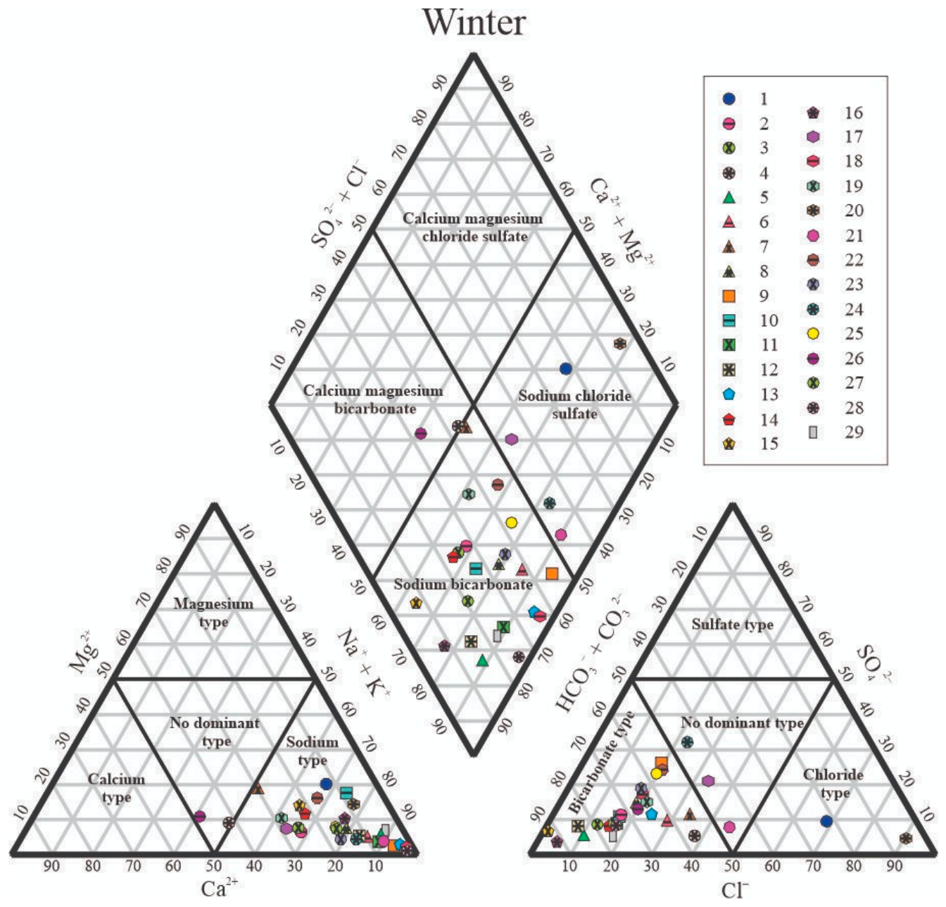
Figure 7.
Annual stability of predictive quality models for spring, winter and winter–spring. a, d, and g) electrical conductivity (E.C.) vs. original sodium adsorption ratio (SARor); b, e, and h) E.C. vs. corrected (SARco); and c, f, and i) E.C. vs. adjusted (SARad).
Figure 7.
Annual stability of predictive quality models for spring, winter and winter–spring. a, d, and g) electrical conductivity (E.C.) vs. original sodium adsorption ratio (SARor); b, e, and h) E.C. vs. corrected (SARco); and c, f, and i) E.C. vs. adjusted (SARad).
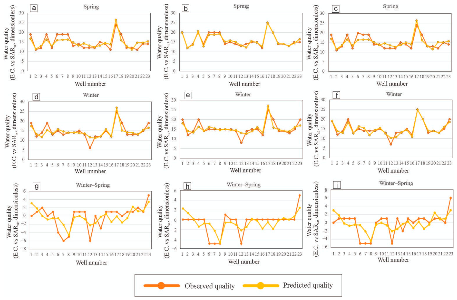

Table 1.
Spatial Variability of 17 Physicochemical Parameters for Spring.
| Well number | pH | E.C. | TDS | Temp | Sal | s.l. | Na+ | Ca2+ | Mg2+ | K+ | Cl– | SO42– | CO32– | HCO3– | SARor | SARco | SARad |
|---|---|---|---|---|---|---|---|---|---|---|---|---|---|---|---|---|---|
| (Dim.) | (µS cm–1) | (ppt) | (°C) | (% NaCl) | (m) | (mEq L–1) | (Dimensionless) | ||||||||||
| 1 | 7.13 | 4580 | 2.30 | 29.90 | 3.00 | 2.70 | 47.85 | 16.97 | 5.84 | 0.10 | 22.99 | 7.70 | 0.00 | 6.66 | 14.17 | 39.82 | 20.59 |
| 2 | 7.75 | 700 | 0.35 | 31.80 | 0.40 | – | 6.09 | 4.59 | 1.48 | 0.12 | 0.99 | 1.02 | 0.00 | 8.23 | 3.49 | 8.67 | 5.03 |
| 3 | 7.63 | 680 | 0.34 | 32.80 | 0.30 | – | 5.22 | 4.39 | 0.91 | 0.07 | 0.42 | 0.35 | 0.00 | 8.23 | 3.21 | 7.81 | 4.87 |
| 4 | 7.35 | 1400 | 0.69 | 40.10 | 1.50 | 4.55 | 6.52 | 20.96 | 4.61 | 1.23 | 7.05 | 1.35 | 0.00 | 10.58 | 1.82 | 5.71 | 3.19 |
| 5 | 8.00 | 1120 | 0.56 | 27.00 | 0.60 | 4.52 | 12.61 | 1.40 | 1.23 | 0.05 | 0.56 | 0.62 | 0.00 | 12.54 | 11.00 | 25.09 | 13.52 |
| 6 | 7.55 | 3390 | 1.69 | 27.80 | 1.60 | 2.80 | 36.10 | 6.99 | 2.14 | 0.05 | 6.77 | 10.20 | 0.00 | 10.98 | 16.90 | 45.10 | 25.56 |
| 7 | 7.51 | 1980 | 0.99 | 35.10 | 1.00 | – | 8.70 | 14.47 | 2.88 | 0.06 | 5.22 | 3.37 | 0.00 | 6.66 | 2.95 | 8.21 | 4.72 |
| 8 | 7.42 | 1000 | 0.49 | 29.40 | 0.50 | 3.59 | 12.61 | 3.24 | 1.23 | 0.07 | 1.97 | 2.04 | 0.00 | 9.41 | 8.43 | 20.04 | 11.70 |
| 9 | 7.72 | 2750 | 1.39 | 28.30 | 1.40 | 2.75 | 33.93 | 3.29 | 1.40 | 0.06 | 3.81 | 11.24 | 0.00 | 11.76 | 22.15 | 53.67 | 30.67 |
| 10 | 7.78 | 2580 | 1.28 | 28.10 | 1.40 | 2.52 | 30.45 | 5.99 | 2.96 | 0.09 | 4.23 | 7.08 | 0.00 | 10.19 | 14.39 | 38.00 | 19.90 |
| 11 | 7.66 | 2650 | 1.31 | 30.30 | 1.40 | 2.17 | 33.06 | 6.49 | 1.97 | 0.05 | 9.03 | 4.33 | 0.00 | 9.80 | 16.07 | 41.69 | 23.82 |
| 12 | 7.80 | 1470 | 0.74 | 30.70 | 0.70 | 2.70 | 20.88 | 5.49 | 1.48 | 0.05 | 2.26 | 3.54 | 0.00 | 10.19 | 11.18 | 28.65 | 16.95 |
| 13 | 7.85 | 1840 | 0.89 | 28.80 | 1.00 | 4.59 | 31.75 | 1.85 | 1.73 | 0.04 | 2.82 | 4.16 | 0.00 | 11.37 | 23.75 | 54.58 | 28.70 |
| 14 | 7.23 | 1850 | 0.94 | 27.00 | 1.00 | 3.16 | 15.66 | 9.98 | 2.80 | 0.04 | 4.80 | 4.66 | 0.00 | 9.02 | 6.20 | 17.16 | 9.60 |
| 15 | 7.39 | 870 | 0.40 | 27.50 | 0.60 | 3.54 | 9.13 | 2.69 | 1.07 | 0.06 | 0.42 | 1.39 | 0.00 | 11.76 | 6.66 | 16.14 | 9.43 |
| 16 | 7.29 | 1090 | 0.55 | 27.90 | 0.70 | 4.27 | 14.35 | 2.35 | 2.55 | 0.07 | 0.56 | 2.50 | 0.00 | 11.76 | 9.17 | 22.96 | 11.14 |
| 17 | 7.96 | 1970 | 0.99 | 29.30 | 1.10 | 4.78 | 30.88 | 1.05 | 0.91 | 0.08 | 2.68 | 5.83 | 0.00 | 12.94 | 31.25 | 65.55 | 37.53 |
| 18 | 8.23 | 1230 | 0.59 | 29.50 | 0.70 | 3.32 | 20.44 | 0.45 | 0.99 | 0.09 | 1.97 | 3.33 | 0.00 | 9.80 | 24.12 | 45.32 | 25.56 |
| 19 | 7.30 | 1000 | 0.51 | 29.10 | 0.60 | 2.86 | 8.70 | 6.99 | 1.89 | 0.06 | 1.27 | 1.92 | 0.00 | 10.19 | 4.13 | 11.18 | 6.46 |
| 20 | 7.32 | 14910 | 7.46 | 31.00 | 8.20 | 1.98 | 117.44 | 20.46 | 33.74 | 1.38 | 3.81 | 14.16 | 0.00 | 10.00 | 22.56 | 74.11 | 26.71 |
| 21 | 7.62 | 3450 | 1.59 | 30.90 | 1.90 | 3.05 | 40.89 | 8.98 | 2.96 | 0.08 | 1.97 | 4.58 | 0.00 | 12.74 | 16.73 | 47.46 | 25.90 |
| 22 | 7.35 | 1820 | 0.92 | 29.20 | 1.00 | 4.32 | 19.14 | 5.49 | 3.21 | 0.09 | 1.13 | 6.77 | 0.00 | 11.76 | 9.18 | 24.97 | 12.59 |
| 23 | 7.45 | 1320 | 0.66 | 32.50 | 0.80 | – | 19.14 | 4.84 | 1.23 | 0.08 | 1.13 | 4.58 | 0.00 | 10.19 | 10.98 | 27.57 | 16.64 |
| 24 | 7.54 | 1640 | 0.80 | 30.50 | 0.90 | – | 22.18 | 3.59 | 1.40 | 0.04 | 1.27 | 6.00 | 0.00 | 9.41 | 14.04 | 33.47 | 19.34 |
| 25 | 7.41 | 1520 | 0.76 | 29.20 | 0.90 | 5.89 | 17.40 | 5.99 | 1.65 | 0.06 | 1.27 | 5.83 | 0.00 | 9.60 | 8.91 | 23.02 | 13.47 |
| 26 | 6.90 | 560 | 0.27 | 29.80 | 0.40 | – | 2.26 | 4.99 | 0.82 | 0.10 | 0.42 | 0.75 | 0.00 | 7.84 | 1.33 | 3.29 | 2.09 |
| 27 | 8.23 | 960 | 0.51 | 28.80 | 0.70 | 2.98 | 9.57 | 4.64 | 1.40 | 0.06 | 1.69 | 2.42 | 0.00 | 9.80 | 5.51 | 13.95 | 8.18 |
| 28 | 8.00 | 1410 | 0.72 | 30.20 | 0.90 | 3.01 | 26.97 | 1.20 | 0.66 | 0.06 | 1.97 | 1.87 | 0.00 | 13.33 | 28.00 | 58.78 | 35.85 |
| 29 | 7.80 | 1870 | 0.93 | 28.50 | 1.20 | 2.72 | 22.62 | 3.49 | 0.66 | 0.07 | 4.65 | 3.75 | 0.00 | 10.58 | 15.70 | 36.99 | 24.01 |
| Bold = extreme value |
|||||||||||||||||
| – = measurement not applied | |||||||||||||||||
Table 2.
Spatial variability of 17 physicochemical parameters for winter.
| Well number | pH | E.C. | TDS | Temp | Sal | s.l. | Na+ | Ca2+ | Mg2+ | K+ | Cl– | SO42– | CO32– | HCO3– | SARor | SARco | SARad |
|---|---|---|---|---|---|---|---|---|---|---|---|---|---|---|---|---|---|
| (Dim.) | (µS cm–1) | (ppt) | (°C) | (% NaCl) | (m) | (mEq L–1) | (Dimensionless) | ||||||||||
| 1 | 6.75 | 4440 | 2.21 | 27.60 | 2.80 | 1.65 | 69.60 | 12.97 | 20.98 | 0.12 | 18.48 | 5.41 | 0.00 | 12.15 | 16.89 | 45.50 | 20.12 |
| 2 | 6.94 | 1230 | 0.61 | 28.00 | 0.80 | – | 21.31 | 7.98 | 2.14 | 0.12 | 1.97 | 2.81 | 0.00 | 17.44 | 9.47 | 10.30 | 15.98 |
| 3 | 6.97 | 1270 | 0.65 | 28.10 | 0.80 | – | 20.88 | 7.98 | 2.47 | 0.13 | 2.54 | 2.91 | 0.00 | 23.91 | 9.13 | 9.94 | 15.53 |
| 4 | 6.73 | 1780 | 0.89 | 27.50 | 1.10 | 3.13 | 17.40 | 15.97 | 3.54 | 1.19 | 4.09 | 1.25 | 0.00 | 12.54 | 5.57 | 5.61 | 9.73 |
| 5 | 7.09 | 1030 | 0.50 | 23.10 | 0.60 | 2.35 | 26.10 | 1.80 | 1.73 | 0.12 | 1.27 | 1.46 | 0.00 | 21.17 | 19.66 | 28.35 | 24.97 |
| 6 | 7.30 | 2460 | 1.23 | 25.90 | 1.50 | 2.18 | 52.20 | 5.99 | 3.29 | 0.10 | 5.78 | 4.06 | 0.00 | 25.09 | 24.23 | 50.84 | 35.62 |
| 7 | 6.98 | 1780 | 0.90 | 27.60 | 1.10 | – | 23.92 | 13.97 | 8.97 | 0.08 | 4.23 | 3.02 | 0.00 | 14.11 | 7.06 | 9.38 | 9.99 |
| 8 | 7.20 | 1060 | 0.53 | 27.80 | 0.60 | 2.16 | 24.36 | 4.24 | 2.47 | 0.09 | 1.27 | 2.08 | 0.00 | 9.21 | 13.30 | 21.00 | 17.47 |
| 9 | 7.38 | 2170 | 1.09 | 27.90 | 1.40 | 1.54 | 56.55 | 2.69 | 1.65 | 0.04 | 3.95 | 11.03 | 0.00 | 22.93 | 38.38 | 58.46 | 53.07 |
| 10 | 7.40 | 1670 | 0.85 | 26.50 | 1.00 | 1.36 | 37.41 | 4.44 | 9.05 | 0.10 | 2.40 | 3.33 | 0.00 | 21.76 | 14.40 | 44.99 | 16.79 |
| 11 | 7.31 | 1120 | 0.58 | 27.80 | 0.70 | 1.42 | 30.01 | 2.59 | 1.32 | 0.09 | 1.69 | 1.87 | 0.00 | 15.29 | 21.46 | 39.69 | 29.61 |
| 12 | 7.44 | 1390 | 0.70 | 26.00 | 0.80 | 1.45 | 32.62 | 4.59 | 2.22 | 0.09 | 1.83 | 4.27 | 0.00 | 42.34 | 17.68 | 35.12 | 27.67 |
| 13 | 7.35 | 1340 | 0.68 | 25.90 | 0.80 | 3.62 | 38.71 | 1.15 | 1.32 | 0.08 | 2.26 | 2.29 | 0.00 | 12.35 | 34.88 | 51.27 | 40.55 |
| 14 | 6.98 | 1670 | 0.84 | 27.00 | 1.30 | 1.83 | 27.40 | 8.98 | 4.94 | 0.07 | 1.69 | 2.00 | 0.00 | 17.64 | 10.39 | 19.00 | 15.19 |
| 15 | 7.19 | 600 | 0.31 | 23.90 | 0.40 | 1.95 | 10.87 | 3.79 | 2.47 | 0.12 | 0.04 | 0.92 | 0.00 | 11.96 | 6.15 | 17.49 | 8.22 |
| 16 | 6.90 | 860 | 0.44 | 23.70 | 0.50 | 2.24 | 20.88 | 3.49 | 2.88 | 0.13 | 0.71 | 1.25 | 0.00 | 28.62 | 11.70 | 27.28 | 15.88 |
| 17 | 7.09 | 1540 | 0.77 | 21.70 | 0.90 | 2.33 | 27.84 | 12.48 | 3.29 | 0.10 | 3.67 | 4.79 | 0.00 | 10.19 | 9.91 | 89.92 | 15.89 |
| 18 | 8.09 | 1090 | 0.55 | 26.90 | 0.70 | 2.70 | 33.06 | 0.55 | 0.82 | 0.08 | 1.41 | 2.60 | 0.00 | 9.60 | 39.92 | 43.66 | 43.02 |
| 19 | 6.96 | 920 | 0.47 | 26.00 | 0.60 | 1.92 | 16.09 | 7.49 | 2.80 | 0.07 | 1.27 | 1.87 | 0.00 | 7.84 | 7.10 | 10.82 | 10.12 |
| 20 | 7.06 | 10230 | 5.13 | 27.20 | 8.30 | 1.29 | 213.14 | 23.95 | 40.32 | 1.85 | 119.88 | 13.12 | 0.00 | 13.92 | 37.60 | 78.07 | 44.89 |
| 21 | 7.21 | 2300 | 1.18 | 26.70 | 1.50 | 2.13 | 52.20 | 3.74 | 2.39 | 0.08 | 6.49 | 2.39 | 0.00 | 13.72 | 29.82 | 43.00 | 39.60 |
| 22 | 7.10 | 1660 | 0.83 | 27.80 | 1.00 | 1.90 | 30.01 | 7.49 | 7.32 | 0.07 | 2.54 | 6.25 | 0.00 | 14.11 | 11.03 | 27.43 | 14.18 |
| 23 | 7.14 | 1200 | 0.60 | 28.40 | 0.70 | – | 25.66 | 5.49 | 1.48 | 0.07 | 1.69 | 3.75 | 0.00 | 12.35 | 13.75 | 28.90 | 21.40 |
| 24 | 7.23 | 1450 | 0.73 | 29.10 | 0.90 | – | 31.75 | 4.99 | 1.81 | 0.07 | 1.83 | 5.31 | 0.00 | 7.45 | 17.22 | 33.50 | 23.39 |
| 25 | 7.18 | 1340 | 0.68 | 27.70 | 0.80 | 6.80 | 28.27 | 5.99 | 3.04 | 0.08 | 1.97 | 4.79 | 0.00 | 11.76 | 13.30 | 24.14 | 18.65 |
| 26 | 6.64 | 930 | 0.47 | 28.40 | 0.60 | – | 9.57 | 11.48 | 2.63 | 0.12 | 1.97 | 2.67 | 0.00 | 13.52 | 3.60 | 3.99 | 6.24 |
| 27 | 7.18 | 1030 | 0.53 | 26.90 | 0.60 | 2.98 | 22.18 | 4.74 | 2.22 | 0.12 | 1.27 | 1.87 | 0.00 | 16.86 | 11.89 | 15.29 | 17.44 |
| 28 | 7.81 | 1580 | 0.80 | 26.00 | 1.00 | 2.03 | 47.85 | 0.95 | 0.74 | 0.13 | 2.82 | 2.91 | 0.00 | 25.48 | 52.07 | 64.19 | 66.91 |
| 29 | 7.53 | 2490 | 1.25 | 27.50 | 1.60 | 1.98 | 56.55 | 2.84 | 4.61 | 0.10 | 5.78 | 3.75 | 0.00 | 51.74 | 29.29 | 50.62 | 35.81 |
| Bold = extreme value |
|||||||||||||||||
| – = measurement not applied | |||||||||||||||||
Table 3.
Pearson (Pr) and Spearman (Sr) correlation coefficients between the physicochemical variables influencing irrigation water quality in spring.
Table 3.
Pearson (Pr) and Spearman (Sr) correlation coefficients between the physicochemical variables influencing irrigation water quality in spring.
| Variable | pH | E.C. | TDS | Temp | Sal | s.l. | Na+ | Ca2+ | Mg2+ | K+ | Cl– | SO42– | HCO3– |
|---|---|---|---|---|---|---|---|---|---|---|---|---|---|
| pH | |||||||||||||
| E.C. | –0.008 | ||||||||||||
| TDS | –0.011 | 0.997 | |||||||||||
| Temp | –0.060 | –0.012 | –0.031 | ||||||||||
| Sal | –0.073 | 0.933 | 0.935 | 0.032 | |||||||||
| s.l. | –0.022 | –0.463 | –0.472 | –0.171 | –0.406 | ||||||||
| Na+ | 0.192 | 0.859 | 0.853 | –0.113 | 0.782 | –0.484 | |||||||
| Ca2+ | –0.573 | 0.426 | 0.438 | 0.324 | 0.499 | –0.415 | 0.080 | ||||||
| Mg2+ | –0.465 | 0.544 | 0.554 | 0.100 | 0.600 | –0.228 | 0.284 | 0.765 | |||||
| K+ | –0.266 | –0.014 | –0.021 | 0.381 | 0.142 | –0.122 | –0.033 | 0.196 | 0.175 | ||||
| Cl– | 0.042 | 0.775 | 0.772 | 0.058 | 0.802 | –0.490 | 0.571 | 0.478 | 0.469 | –0.043 | |||
| SO42– | –0.125 | 0.843 | 0.856 | –0.144 | 0.763 | –0.376 | 0.801 | 0.326 | 0.482 | 0.009 | 0.534 | ||
| HCO3– | 0.391 | 0.164 | 0.164 | –0.369 | 0.228 | 0.283 | 0.347 | –0.397 | –0.106 | –0.084 | –0.077 | 0.081 | |
| SARor | 0.489 | 0.619 | 0.611 | –0.175 | 0.531 | –0.136 | 0.880 | –0.333 | –0.068 | –0.074 | 0.366 | 0.563 | 0.541 |
| SARco | 0.351 | 0.695 | 0.687 | –0.126 | 0.604 | –0.271 | 0.927 | –0.220 | 0.035 | –0.046 | 0.406 | 0.638 | 0.489 |
| SARad | 0.452 | 0.668 | 0.659 | –0.161 | 0.576 | –0.217 | 0.909 | –0.277 | –0.054 | –0.087 | 0.398 | 0.610 | 0.545 |
| Boxed = | n = 23, crP = |0.413|, crS = |0.418| | ||||||||||||
| Without Boxed = |
n = 29, crP = |0.367|, crS = |0.370| | ||||||||||||
| A = | Spearman correlation (Sr). | ||||||||||||
| A = | Pearson correlation (Pr). | ||||||||||||
| Bold = | Significant correlation. | ||||||||||||
Table 4.
Pearson (Pr) and Spearman (Sr) correlation coefficients between the physicochemical variables influencing irrigation water quality in winter.
Table 4.
Pearson (Pr) and Spearman (Sr) correlation coefficients between the physicochemical variables influencing irrigation water quality in winter.
| Variable | pH | E.C. | TDS | Temp | Sal | s.l. | Na+ | Ca2+ | Mg2+ | K+ | Cl– | SO42– | HCO3– |
|---|---|---|---|---|---|---|---|---|---|---|---|---|---|
| pH | |||||||||||||
| E.C. | 0.150 | ||||||||||||
| TDS | 0.158 | 0.999 | |||||||||||
| Temp | –0.178 | 0.095 | 0.090 | ||||||||||
| Sal | 0.116 | 0.992 | 0.991 | 0.112 | |||||||||
| s.l. | –0.096 | –0.364 | –0.362 | –0.288 | –0.349 | ||||||||
| Na+ | 0.592 | 0.738 | 0.740 | –0.079 | 0.723 | –0.372 | |||||||
| Ca2+ | –0.742 | 0.305 | 0.304 | 0.291 | 0.318 | –0.181 | –0.261 | ||||||
| Mg2+ | –0.452 | 0.482 | 0.484 | –0.046 | 0.471 | –0.310 | 0.044 | 0.703 | |||||
| K+ | –0.356 | –0.066 | –0.069 | –0.274 | –0.076 | 0.083 | –0.200 | 0.197 | 0.207 | ||||
| Cl– | 0.008 | 0.906 | 0.906 | 0.136 | 0.902 | –0.230 | 0.611 | 0.377 | 0.438 | 0.105 | |||
| SO42– | 0.192 | 0.635 | 0.639 | 0.349 | 0.620 | –0.351 | 0.628 | 0.289 | 0.274 | –0.265 | 0.624 | ||
| HCO3– | 0.186 | 0.243 | 0.245 | –0.166 | 0.240 | –0.290 | 0.211 | –0.210 | 0.036 | 0.269 | 0.199 | 0.032 | |
| SARor | 0.741 | 0.377 | 0.377 | –0.158 | 0.365 | –0.123 | 0.860 | –0.625 | –0.389 | –0.184 | 0.265 | 0.334 | 0.229 |
| SARco | 0.708 | 0.499 | 0.501 | –0.333 | 0.479 | –0.229 | 0.867 | –0.370 | –0.099 | –0.086 | 0.424 | 0.511 | 0.139 |
| SARad | 0.707 | 0.369 | 0.370 | –0.101 | 0.358 | –0.088 | 0.826 | –0.576 | –0.447 | –0.149 | 0.290 | 0.352 | 0.213 |
| Boxed = | n = 23, crP = |0.413|, crS = |0.418| | ||||||||||||
| Without boxed = | n = 29, crP = |0.367|, crS = |0.370| | ||||||||||||
| A = | Spearman correlation (Sr). | ||||||||||||
| A = | Pearson correlation (Pr). | ||||||||||||
| Bold = | Significant correlation. | ||||||||||||
Table 5.
Pearson (Pr) and Spearman (Sr) repeated measures correlation coefficients between the physicochemical variables influencing irrigation water quality (rate of change from winter minus spring).
Table 5.
Pearson (Pr) and Spearman (Sr) repeated measures correlation coefficients between the physicochemical variables influencing irrigation water quality (rate of change from winter minus spring).
| Variable | pH | E.C. | TDS | Temp | Sal | s.l. | Na+ | Ca2+ | Mg2+ | K+ | Cl– | SO42– | HCO3– |
|---|---|---|---|---|---|---|---|---|---|---|---|---|---|
| pH | |||||||||||||
| E.C. | –0.081 | ||||||||||||
| TDS | –0.024 | 0.977 | |||||||||||
| Temp | 0.475 | –0.067 | –0.082 | ||||||||||
| Sal | 0.203 | 0.563 | 0.561 | 0.171 | |||||||||
| s.l. | 0.202 | –0.134 | –0.126 | 0.307 | 0.001 | ||||||||
| Na+ | 0.059 | 0.255 | 0.218 | 0.110 | 0.571 | 0.218 | |||||||
| Ca2+ | 0.039 | 0.228 | 0.269 | –0.065 | 0.432 | –0.367 | –0.126 | ||||||
| Mg2+ | 0.091 | 0.005 | –0.070 | 0.248 | 0.333 | –0.023 | 0.240 | 0.269 | |||||
| K+ | –0.068 | –0.122 | –0.127 | –0.225 | 0.109 | 0.124 | 0.103 | 0.193 | 0.121 | ||||
| Cl– | –0.014 | 0.182 | 0.221 | –0.106 | 0.392 | 0.116 | 0.159 | 0.623 | 0.113 | 0.054 | |||
| SO42– | –0.073 | 0.773 | 0.812 | –0.198 | 0.565 | –0.192 | 0.276 | 0.455 | –0.047 | 0.001 | 0.434 | ||
| HCO3– | –0.138 | 0.204 | 0.117 | 0.031 | 0.361 | 0.053 | 0.473 | –0.190 | 0.150 | 0.299 | 0.030 | 0.161 | |
| SARor | 0.083 | 0.036 | 0.075 | 0.014 | 0.311 | 0.416 | 0.671 | –0.276 | –0.393 | 0.155 | 0.152 | 0.162 | 0.296 |
| SARco | –0.045 | 0.025 | –0.086 | 0.008 | 0.193 | –0.343 | 0.356 | 0.071 | 0.524 | 0.281 | 0.114 | 0.005 | 0.605 |
| SARad | 0.018 | 0.083 | 0.120 | –0.101 | 0.321 | 0.370 | 0.623 | –0.218 | –0.455 | 0.123 | 0.217 | 0.240 | 0.322 |
| Boxed = | n = 23, crP = |0.413|, crS = |0.418| | ||||||||||||
| Without Boxed = |
n = 29, crP = |0.367|, crS = |0.370| | ||||||||||||
| A = | Spearman correlation (Sr). | ||||||||||||
| A = | Pearson correlation (Pr). | ||||||||||||
| Bold = | Significant correlation. | ||||||||||||
Table 6.
p-values from the paired tests for 17 physicochemical variables, obtained in spring and winter.
Table 6.
p-values from the paired tests for 17 physicochemical variables, obtained in spring and winter.
| Variable | p–valor | |
|---|---|---|
| t–test | Wilcoxon–test | |
| pH | 7.513 | – |
| E.C. | – | 0.003 |
| TDS | – | 0.003 |
| Temp | – | 4.768 |
| Sal | – | 0.101 |
| s.l. | – | 6.199 |
| Na+ | – | 1.000 |
| Ca2+ | – | 0.503 |
| Mg2+ | – | 0.001 |
| K+ | – | 6.563 |
| Cl– | – | 0.756 |
| SO42– | – | 0.001 |
| CO32– | – | Identical samples idénticas |
| HCO3– | – | 1.000 |
| SARor | – | 2.000 |
| SARco | 0.010 | – |
| SARad | – | 4.600 |
Bold = significant p–valor.
Table 7.
Performance metrics applied between observed and predicted irrigation water quality values.
Table 7.
Performance metrics applied between observed and predicted irrigation water quality values.
| Variable | Spring (E.C. vs SARor) |
Spring (E.C. vs SARco) |
Spring (E.C. vs SARad) |
Winter (E.C. vs SARor) |
Winter (E.C. vs SARco) |
Winter (E.C. vs SARad) |
Winter–Spring (E.C. vs SARor) |
Winter–Spring (E.C. vs SARco) |
Winter–Spring (E.C. vs SARad) |
|
|---|---|---|---|---|---|---|---|---|---|---|
| Normality [p(normal)] | 0.105 | 0.154 | 0.245 | 0.063 | 0.274 | 0.030 | 0.002 | 0.153 | 0.258 | |
| Homoscedasticity [p(value)] |
Breusch–Pagan | 0.079 | 0.040 | 0.126 | 0.762 | 0.878 | – | – | 0.358 | 0.629 |
| White | 0.213 | – | 0.214 | 0.766 | 0.812 | – | – | 0.422 | 0.460 | |
| Homogeneity (dimensionless) | 0.000 | – | 0.000 | 0.000 | 0.000 | – | – | 0.000 | 0.000 | |
| Independence [p(value)] |
Durbin–Watson | 0.942 | – | 0.878 | 0.807 | 0.632 | – | – | 0.203 | 0.500 |
| Box–Pierce | 0.801 | – | 0.679 | 0.457 | 0.308 | – | – | 0.271 | 0.283 | |
| Ljung–Box | 0.663 | – | 0.527 | 0.249 | 0.152 | – | – | 0.117 | 0.126 | |
| Mc Leod–Li | 0.415 | – | 0.847 | 0.442 | 0.376 | – | – | 0.334 | 0.036 | |
| Minimal multicolinearity (dimensionless) |
pH | 1.116 | – | 1.116 | 1.070 | 1.070 | – | – | 2.744 | – |
| E.C. | 1.372 | – | 1.372 | 1.217 | 1.217 | – | – | 25.412 | – | |
| Temp | 1.053 | – | 1.053 | 1.114 | 1.114 | – | – | – | – | |
| S.l. | 1.276 | – | 1.276 | 1.094 | 1.094 | – | – | – | – | |
| Performance tests (dimensionless) |
Sr | 0.789 | 0.922 | 0.800 | 0.842 | 0.857 | 0.887 | 0.653 | 0.575 | 0.470 |
| R2 | 0.623 | 0.851 | 0.639 | 0.708 | 0.735 | 0.786 | 0.427 | 0.330 | 0.221 | |
| RMSE | 2.033 | 0.804 | 1.937 | 1.955 | 1.976 | 1.294 | 2.002 | 1.661 | 1.947 | |
| MEC | 4.134 | 0.646 | 3.751 | 3.823 | 3.904 | 1.673 | 4.009 | 2.760 | 3.790 | |
| NSE | 0.990 | 0.998 | 0.990 | 0.991 | 0.990 | 0.996 | 1.000 | 0.998 | 1.000 | |
| PBIAS | ||||||||||
| ME | ||||||||||
Bold = not significant value. – = test not applied.
Disclaimer/Publisher’s Note: The statements, opinions and data contained in all publications are solely those of the individual author(s) and contributor(s) and not of MDPI and/or the editor(s). MDPI and/or the editor(s) disclaim responsibility for any injury to people or property resulting from any ideas, methods, instructions or products referred to in the content. |
© 2026 by the authors. Licensee MDPI, Basel, Switzerland. This article is an open access article distributed under the terms and conditions of the Creative Commons Attribution (CC BY) license (http://creativecommons.org/licenses/by/4.0/).
Copyright: This open access article is published under a Creative Commons CC BY 4.0 license, which permit the free download, distribution, and reuse, provided that the author and preprint are cited in any reuse.