

Submitted:
08 October 2026
Posted:
09 October 2026
You are already at the latest version
Abstract
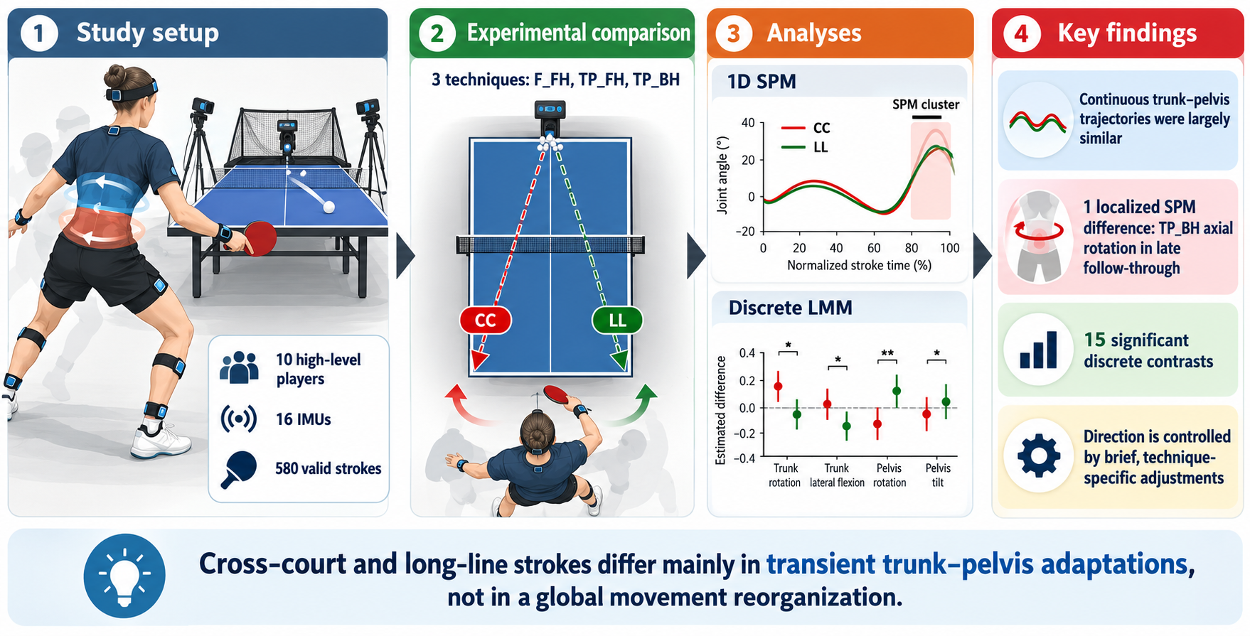
Stroke direction in table tennis may require technique-specific adaptations of trunk–pelvis motion, but the timing and magnitude of these adjustments remain unclear. This study compared cross-court (CC) and long-line (LL) kinematics during forehand counter-topspin (F_FH), forehand topspin (TP_FH), and backhand topspin (TP_BH). Ten high-level players performed both target directions while whole-body kinematics were recorded using a 16-sensor inertial measurement unit system. A total of 580 valid strokes were analysed. Continuous torso–pelvis flexion–extension, lateral bending, and axial rotation trajectories were compared using one-dimensional statistical parametric mapping (SPM), while discrete variables were analysed using linear mixed-effects models with false discovery rate correction. CC and LL trajectories were largely similar across techniques; only a late follow-through axial-rotation difference was identified for TP_BH (SPM cluster, p = 0.030). Discrete analyses revealed technique-specific differences in selected contact angles, ranges of motion, trunk–pelvis separation measures, and angular velocities, with predominantly negligible-to-small effect sizes and no variable differentiating all three techniques. Stroke direction therefore appears to be accommodated mainly through brief, technique-specific kinematic adjustments rather than a global alteration of torso–pelvis movement patterns, highlighting the complementary information provided by continuous and discrete biomechanical analyses.
Keywords:
table tennis
; trunk–pelvis kinematics
; statistical parametric mapping
; inertial measurement units
; stroke direction
; sports biomechanics
1. Introduction
Low back pain (LBP) is among the most prevalent musculoskeletal complaints in athletes, although reported prevalence varies considerably across sporting disciplines and study designs [1] . Sports characterised by repeated, high-velocity trunk rotation and asymmetrical loading—including tennis, golf, baseball, cricket and hockey—may expose the lumbar spine to recurrent combinations of axial rotation, lateral bending and flexion, particularly when these motions occur under substantial muscular force or fatigue [1,2]. Such repeated multidirectional loading is considered a plausible mechanical contributor to lumbar tissue overuse and the development or recurrence of LBP [2]. Although table tennis is a non-contact sport, its principal strokes involve whole-body kinetic chain actions in which rapid trunk rotation transfers energy from the lower limbs and pelvis to the racket-bearing arm [3]. Consequently, the large number of high-speed, asymmetrical strokes performed during training and competition may produce substantial cumulative lumbar loading, despite the relatively low external-impact demands of the sport [4,5].
Table tennis performance depends on coordinated energy transfer through the kinetic chain, in which forces generated by the lower limbs are transmitted through the pelvis and trunk to the racket-bearing arm. Lower-trunk axial rotation contributes directly to racket speed, and advanced players have been shown to derive a greater proportion of racket velocity from this motion than intermediate players [6]. Stroke direction further modifies this coordination strategy: during cross-court topspin forehands, players demonstrate greater lumbar flexion and lateral bending ranges of motion, along with greater pelvic axial rotation, peak moments, and maximum joint angles than during long-line strokes [5]. These findings indicate that cross-court and long-line strokes require distinct trunk–pelvis movement patterns and different strategies of weight transfer and energy production [5]. However, the simultaneous occurrence of lumbar flexion, lateral bending and axial rotation may increase tissue loading because coupled multiplanar motion imposes greater mechanical demands than isolated single-plane movement. Experimental evidence also indicates that repeated combined flexion, lateral bending and axial rotation can damage the posterolateral annulus, although such findings should be interpreted as mechanistic rather than direct evidence of injury during table tennis [7] . Accordingly, repeated high-velocity rotational strokes may generate substantial cumulative lumbar exposure, particularly when large ranges of motion are combined with rapid rotation, muscular force, and limited recovery.
Cross-court (CC) and long-line (LL) strokes serve different tactical purposes and require players to modify whole-body orientation and racket trajectory to direct the ball towards distinct target areas. Previous studies have reported direction-dependent differences in lower- and upper-body rotation, knee and elbow configuration, body alignment relative to the table, and racket inclination at impact, with LL forehands generally exhibiting a more pronounced racket inclination than CC forehands [8,9]. These findings suggest that stroke direction may also modify pelvis orientation, thorax–pelvis coordination and follow-through mechanics. However, the available literature remains limited and has predominantly examined isolated joint variables, racket-arm mechanics, or discrete values extracted at impact, maximum racket velocity, or other selected events [8,9,10]. Studies of the topspin backhand have likewise identified direction-specific differences in wrist and shoulder mechanics, thorax–pelvis rotational velocity and joint moments but have not comprehensively characterised lumbar motion throughout the complete stroke cycle. Although continuous one-dimensional analyses have recently been introduced, they have generally been restricted to a single stroke type, selected movement phases or a limited set of trunk and pelvic variables [5] . Consequently, it remains unclear when, during the stroke, CC and LL techniques diverge, and whether discrete outcome measures adequately capture these differences. Although coaches routinely distinguish between CC and LL execution, three-dimensional lumbar and trunk–pelvis kinematics have not yet been comprehensively quantified across several stroke types and all principal movement phases. This limitation is clinically relevant because target-dependent adaptations may alter the magnitude, direction and timing of lumbar flexion, lateral bending and axial rotation, thereby influencing the cumulative mechanical loading imposed on the spine [5].
Traditional biomechanical analyses frequently reduce complex movement waveforms to discrete variables, such as maximum angles, ranges of motion or values recorded at predefined events. Although these measures are readily interpretable, they may overlook differences in movement timing, duration, and waveform shape, as well as transient adaptations that occur outside the selected instants. Statistical parametric mapping (SPM) or its nonparametric version (SnPM) enables hypothesis testing across the entire normalised movement cycle while accounting for the temporal dependence between adjacent data points and controlling the trajectory-wide Type I error rate [11,12]. It can therefore identify not only whether two stroke conditions differ, but also the specific portions of the backswing, forward swing and follow-through in which those differences occur. This approach is particularly relevant to lumbar and trunk–pelvis kinematics, where potentially meaningful rotational or multiplanar adaptations may be brief and may not coincide with the maximum or minimum angle. Despite the growing use of one-dimensional statistical methods in biomechanics, continuous comparisons of CC and LL table tennis strokes remain scarce and have been limited to selected strokes, phases or anatomical variables. No study has yet combined SPM/SnPM with discrete-variable analysis to comprehensively compare three-dimensional lumbar and trunk–pelvis kinematics in the CC and LL directions across several table tennis strokes, leaving uncertainty about whether conventional discrete measures adequately capture direction-dependent movement strategies.
The primary aim of this study was to compare three-dimensional trunk–pelvis kinematics between cross-court (CC) and long-line (LL) table tennis strokes. Specifically, the study sought to determine whether stroke direction affected torso–pelvis flexion–extension, lateral bending, and axial rotation throughout the complete movement cycle. A further aim was to identify the movement phases during which direction-dependent differences occurred and to determine which discrete kinematic variables exhibited the largest differences between CC and LL execution. By combining statistical parametric mapping with discrete-variable analysis, the study also examined whether continuous waveform analysis revealed differences not captured by conventional peak, range-of-motion, or event-based measures.
The following hypotheses were tested:
H1. CC and LL strokes would demonstrate distinct three-dimensional trunk–pelvis kinematic patterns due to their distinct directional and tactical requirements.
H2. CC strokes would be characterised by greater transverse-plane rotation and greater multiplanar motion of the torso–pelvis complex, including lateral bending and flexion, than LL strokes.
H3. The largest direction-dependent differences would occur during the forward-swing and follow-through phases, when racket direction and whole-body rotation are most strongly adjusted to the target.
H4. Statistical parametric mapping would identify significant temporal differences between CC and LL strokes that would not be detected using discrete kinematic variables alone.
The findings may have practical value for coaches, athletes and clinicians by identifying stroke phases and directional techniques associated with greater trunk–pelvis motion. This information could support technique modification, workload management and targeted trunk-conditioning programmes intended to preserve performance while reducing cumulative spinal loading and, potentially, the risk of LBP.
2. Materials and Methods
2.1. Study Design
Controlled laboratory study, cross-sectional, with a within-subject repeated-measures design. Each participant performed all six stroke conditions, with the primary within-subject contrast relating to the target zone to be reached.
2.2. Participants
The study included 10 high-level table tennis players (age: 18.5 ± 5.1 years; body height: 1.72 ± 0.16 m; body mass: 62.71 ± 18.98 kg). The inclusion criteria were a high level of competitiveness, regular participation in table tennis training and competition, and the ability to perform all experimental stroke conditions. Participants were required to be healthy and free from current pain, musculoskeletal injury or any other condition that could affect stroke execution.
The study protocol was approved by the Senate Bioethics Commission of the Wroclaw University of Health and Sport Sciences (approval no. 34/2019) and was conducted in accordance with the Declaration of Helsinki. Written informed consent was obtained from all adult participants before data collection. For participants who were minors, written informed consent was obtained from a parent or legal guardian, together with the participant’s assent, in accordance with the approved study protocol.
2.3. Instrumentation / Measurement Procedure
The whole-body joint angles were measured at every instant of the movement using an IMU system to construct a whole-body representation of the participant, providing access to all relevant joint angles and angular velocities. In parallel, additional tools were used, including force platforms, with their data to be used in future studies.
To measure kinematic data on participants’ movements, the myoMOTION™ IMU system (Noraxon USA Inc., Scottsdale, AZ, USA) was used. It consisted of placing 16 sensors on the participant’s body in accordance with the manufacturer’s protocol (Figure 1). For the present analysis, particular attention was given to the lower-thorax and pelvis segments. The lower-thorax sensor represented the spatial orientation of the lower torso, whereas the pelvis sensor represented pelvic orientation. Flexion–extension, lateral bending, and axial rotation were therefore expressed as the orientation of the torso relative to the pelvis and should not be interpreted as isolated lumbar-spine or intervertebral motion. Sensor placement and calibration were performed by the same experienced technician prior to data collection.
The validity and reliability of IMU-based motion-capture systems for analysing dynamic movements have been demonstrated in previous studies [13]. The sensors were placed symmetrically so that the positive x-coordinate indicated on the sensor label corresponded to an upward orientation of the trunk, head, and pelvis. All participants were checked at the beginning of the measurements, and the system was calibrated. For the sensors located on the limb segments, the positive x-coordinate corresponded to a proximal orientation. For the foot sensor, the x-coordinate was oriented distally (toward the toes). The sensors were placed according to the myoMotion manual protocol. The sampling frequency was 100 Hz per sensor (in a 16-sensor full-body configuration).
The experimental area involved a robot delivering balls under controlled conditions. Kinematic data were recorded using a 16-sensor IMU system (myoMOTION™, Noraxon USA Inc., Scottsdale, AZ, USA) placed on the head, trunk and pelvis, and bilaterally on the upper and lower limbs (Figure 2). All systems were synchronised and calibrated before each test.
The inertial data from the integrated motion sensors, including the joint angles of the body segments of interest, were used to determine the maximum and mean angular velocities. Angular velocity was computed from the difference between the preceding and following angle divided by the time interval separating them ((angle[i+1] − angle[i−1]) / (2·dt)). These included the maximal resultant angular velocity (W_Max) and the maximal angular velocities about the medio-lateral (X), antero-posterior (Y) and vertical (Z) axes — denoted Wmax_FE, Wmax_LB and Wmax_AR, respectively. All angular-velocity parameters were expressed in degrees per second (°/s).
The analysed strokes comprised three offensive techniques:
- forehand topspin (TP_FH) was performed against a backspin ball and typically involved a lower body position, greater knee and trunk flexion, a more pronounced upward racket path, and a longer acceleration phase to generate sufficient lift and topspin.
- backhand topspin (TP_BH) was also performed against a backspin ball, but from the backhand side, with the racket positioned in front of the body, a more compact trunk action, and greater reliance on elbow extension, forearm rotation, and wrist movement.
- counter-topspin forehand (F_FH) was a forehand topspin played against an incoming topspin or lifted ball and was characterised by a more upright posture, a shorter backswing, earlier ball contact, and a more forward-directed racket trajectory than TP_FH.
The player’s movement was divided into three phases within a stroke [14]. The phases and events were identified using an algorithm applied to the hip and hand data. The specific events were: backswing (1), forward swing (2), contact (3) and follow-through (4). The identification of these specific events allowed the different phases of the studied movement to be defined:
- Backswing (z0 → z1): Begins at the ready position (z0), with the handheld high and nearly stationary ahead of the body following the previous stroke and ends at the instant the hand reverses its direction of travel from backwards to forwards (z1). The end of this phase corresponds to the initiation of the forward motion, defined as the earliest acceleration of either the pelvis or the hand along the kinematic chain.
- Forward swing (z1 → z2): Covers the striking phase of the stroke, from the forward motion up to racket–ball contact (z2).
- Follow-through (z2 → z3): Covers the forward motion after contact, relying on a deceleration of the hand velocity, until it reaches a low velocity threshold relative to its peak (z3).
Because racket–ball contact was not measured directly, the contact event (z2) was estimated kinematically as the instant of maximum playing-hand velocity along the principal movement axis determined by principal component analysis (PCA). Previous motion-analysis studies in table tennis have shown that peak racket velocity occurs at or very close to racket–ball impact, supporting the use of peak end-effector velocity as a practical proxy for the contact instant [9,15,16,17].
The tests were conducted in the research laboratory of the AWF University. Testing was carried out over two sessions, with the measurement protocol and the equipment used strictly identical. Before the test, all participants were able to warm up individually, first without a racket, then with a racket, performing forehand and backhand topspin at the table.
All participants performed six conditions. With each stroke divided according to whether a cross-court or a long line target zone was aimed at, they performed three technical strokes: the forehand (fh) topspin, the backhand (bh) topspin and the fh counter-topspin. The players were instructed to aim at a target zone placed in a corner of the table according to the zone (width 20cm, length 30cm) to be reached, cross-court or long line. Participants were instructed to perform the strokes with their maximal force while maintaining a certain degree of accuracy.
During stroke execution, a form was completed by the same experimenter to indicate whether each stroke was valid or not. In case of doubt, video footage was used to verify whether the played ball had indeed reached the target zone. All strokes for which the ball did not reach the target zone were excluded. The balls (Andro Speedball 3S 40+) were delivered using a Newgy Robo-Pong 2055 table tennis robot (Newgy Industries, Gallatin, TN, USA) with spin, speed, direction and frequency settings specific to each stroke. The robot settings were: in topspin fh task: rotation - backspin, speed (determines both speed and spin, where 0 is the minimum and 30 is the maximum) - 11, left position (left most position to which the ball is delivered) - 4, wing (robot’s head angle indicator) - 9.5 and frequency (time interval between balls thrown) - 1.4 s; in topspin bh task: rotation - backspin, speed - 11, right position - 16, wing - 9.5 and frequency - 1.4 s; In fh counter-topspin task: rotation - topspin, speed - 18, left - 4, wing - 8,5 and interval - 1.4 s. These parameters ensured a consistent ball trajectory and timing from one trial to the next.
All participants performed a series of 15 strokes per condition, with at least 5 valid strokes per participant. When the number of valid strokes was insufficient, they performed a second series until the recommended number was reached. Each player completed the experiment with their own racket, and the blades and rubbers used were recorded in a document, along with their characteristics. Plastic balls (Andro Speedball 3S 40+) and a Donic Persson 25 table (Donic, Sportartikel-Vertriebs GmbH, Völklingen, Germany) were used for all trials. Participants were given time to familiarise themselves with the equipment.
2.4. Data Analysis
Following the experimental protocols, all files were exported from the Noraxon myoRESEARCH® MR4 (Noraxon U.S.A., Inc., Scottsdale, AZ, USA) software in C3D format for processing in MATLAB (version R2026a; The MathWorks Inc., Natick, MA, USA). Each file contained the raw IMU data, namely the angular velocities and accelerometer data for each inertial measurement unit. In addition, the export included data processed by the software, namely the joint angles of the various body segments, as well as the positions of virtual markers placed on anatomical landmarks by the software.
The first stage of the MATLAB processing consisted of segmenting each condition file into 15 segments corresponding to the 15 strokes performed within it. To this end, a semi-automatic detection algorithm was developed. This algorithm identified peaks in hand velocity along the principal direction estimated by principal component analysis of the recording; the experimenter then selected the peaks to retain, excluding those corresponding to strokes performed before or after ball delivery by the robot.
The second stage consisted of identifying, for each stroke defined above, the following events:
- Onset of the backswing: identification of the negative velocity peak preceding the ball-contact peak, followed by a backward search from that peak for the first instant at which velocity fell below 8% of the peak’s maximal velocity.
- Onset of the strike: according to the kinematic chain of the movement, the first segment, among those between the hand and the pelvis, to exhibit a forward angular velocity.
- Ball contact (estimated): the instant of maximum playing-hand velocity along the principal movement axis determined by PCA.
- End of the follow-through phase: the first instant after contact at which hand velocity returned below a threshold of 8% of the peak velocity.
At the end of this processing, each initial file was split into 936 new C3D files, each corresponding to a single stroke. In parallel, a file was created indicating whether each trial was valid, based on post hoc visual verification of camera footage recorded after the experiment; this yielded a total of 580 files used for subsequent data analysis.
For the analysis of the 580 files, both discrete and continuous kinematic variables were extracted. Discrete variables included the range of motion (ROM), defined as the difference between the maximum and minimum joint angle over the analysed period; maximum angular velocity (ω_max); mean angular velocity (ω_mean), calculated from the beginning of the arm-swing phase to racket–ball contact; and the separation angle (X-factor, XF). The X-factor represented a separate trunk–pelvis separation measure and should be distinguished from the torso–pelvis relative angular variables described below. It was defined as the angular separation between the pelvis and the line connecting the two acromion landmarks. These variables were calculated either over the entire recording or at specific time points defined relative to the identified movement events.
Continuous torso–pelvis angular trajectories were analysed in three anatomical planes: flexion–extension (FE), lateral bending (LB), and axial rotation (AR). These variables described the relative orientation of the torso with respect to the pelvis and should not be interpreted as isolated intervertebral or lumbar-spine motion. Because the lumbar region forms part of the lower portion of this torso–pelvis complex, these measures were considered relevant to regional lumbar movement but were not lumbar-specific. All angular variables were expressed in degrees, whereas angular velocities were expressed in degrees per second.
2.5. Statistical Analysis
Sample size was determined a priori using the means, standard deviations and distributional characteristics obtained in a previous experiment conducted in a comparable population and under similar measurement conditions [18]. The calculation was based on the expected magnitude and variability of within-subject differences between cross-court (CC) and long-line (LL) strokes, with α = 0.05. Before inferential analysis, the dataset was screened for completeness, coding errors, implausible values and missing observations. Data integrity was additionally assessed by inspecting descriptive statistics and graphical representations, including histograms and boxplots. The distribution of the discrete variables was evaluated using appropriate normality tests together with visual inspection, because formal tests alone may be sensitive to sample size and may not fully reflect the practical suitability of parametric assumptions. The normality of the continuous CC–LL difference trajectories were assessed using the D’Agostino–Pearson omnibus K² test applied across the normalised movement cycle [19].
To test the study hypotheses, two complementary analyses were conducted, each corresponding to the nature of the extracted data. The first focused on scalar data (parameters) related to angles and velocities, while the second examined continuous angular trajectory data (1D). In both cases, the contrast of interest involved a within-subject comparison based on the stroke target zone: cross-court (CC) versus long-line (LL). The significance threshold was set at α = 0.05. Statistical analyses were performed using R (version 4.4.4; R Core Team, 2024) for discrete data and MATLAB (version R2026a; The MathWorks Inc., Natick, MA, USA) for continuous data.
First, for the discrete data, each variable was modelled using a linear mixed-effects model of the following form:
Indicator ~ direction + (1 | subject)
The sole fixed effect was target direction (long-line vs. cross-court), estimated independently within each stroke type (F_FH, TP_FH, TP_BH). A random intercept for each participant was included to account for the non-independence of repeated trials within the same subject [20]. Prior to conducting post-hoc comparisons, model assumptions were verified, and the normality of residuals was confirmed via visual inspection of Q-Q plots. For each variable and stroke type, the effect of target direction (CC and LL) and its associated confidence interval were estimated using estimated marginal means via the “emmeans” package [21]. Effect sizes (Cohen’s d) were calculated by dividing the fixed-effect coefficient estimate by the total standard deviation, defined as the square root of the sum of the residual variance and the random intercept variance [22]. These were interpreted based on standard thresholds from the scientific literature: negligible (|d| < 0.20), small (0.20 ≤ |d| < 0.50), moderate (0.50 ≤ |d| < 0.80), large (|d| ≥ 0.80) [23]. For the discrete-variable analysis, each biomechanical indicator was treated as a separate inferential family. Within each indicator, the three CC–LL contrasts corresponding to F_FH, TP_FH, and TP_BH were adjusted for multiple comparisons using the Benjamini–Hochberg false discovery rate procedure [19]. Statistical significance was determined from the resulting FDR-adjusted p-values (q < 0.05).
Second, the continuous kinematic analysis focused on the relative orientation of the torso with respect to the pelvis in flexion–extension, lateral bending, and axial rotation. These trajectories represented torso–pelvis motion rather than isolated lumbar-spine kinematics. Each angular trajectory was analysed as a single continuous curve over the normalised movement cycle; significant clusters were subsequently classified according to the movement sub-phase in which they occurred (backswing, forward swing, or follow-through), delimited by group-median event landmarks. For each trial, the time series window was time-normalised to 101 data points using linear interpolation. The trials were then averaged within each subject, and the paired difference was calculated for each participant as follows:
Δ(t)=“CC” (t)-“LL” (t),
Statistical inference was based on Statistical Parametric Mapping (SPM), implemented via the “spm1d” module in MATLAB. This approach relies on a one-sample t-test applied to the differences Δ(t), which were tested against zero at each point along the continuum. The critical threshold and cluster-level inference were computed separately for each of the three stroke techniques (F_FH, TP_FH, and TP_BH). The normality of the within-subject CC–LL difference trajectories was assessed separately for each stroke and movement plane using the D’Agostino–Pearson K² test across the normalised stroke cycle. As shown in Supplementary Figure S1, the normality assumption was satisfied for nearly all time points and variables, with only isolated short supra-threshold regions observed, mainly for flexion–extension in F_FH and TP_FH. Because departures from normality were limited in extent and were not systematic across strokes or movement planes, parametric one-dimensional SPM was used for the subsequent CC–LL comparisons. The p-values were obtained through exhaustive recommendations of Pataky et al. (2015), who demonstrated that the distinction between 0D and 1D models is more critical than the distinction between parametric and non-parametric approaches when analysing biomechanical trajectories. Furthermore, this approach has previously been applied to the kinematic analysis of table tennis [24]. Nine continuous SPM comparisons were performed, corresponding to three movement planes (flexion–extension, lateral bending and axial rotation) across three stroke techniques. SPM controlled the family-wise Type I error rate across the temporal continuum within each trajectory. No additional multiplicity correction was applied across the nine separate trajectory-level SPM tests. Accordingly, statistical significance should be interpreted at the level of each individual trajectory rather than as experiment-wide evidence across all nine comparisons.
3. Results
The results presented in this section relate to the comparison, for a given stroke, between the two conditions, namely aiming at a long-line or a cross-court target.
3.1. Angular Trajectory
The mean torso angular trajectories relative to the pelvis for CC and LL execution across the three table tennis techniques are presented in Figure 3. The figure shows flexion–extension, lateral bending and axial rotation over the normalised stroke cycle, together with the corresponding standard-deviation envelopes and any significant temporal clusters identified by the SPM analysis.
For the counter-topspin forehand (F_FH), the CC and LL trajectories were closely matched in all three planes, and the SPM analysis identified no significant differences across the movement cycle. Flexion–extension increased gradually during the backswing, reached its maximum near the transition to the forward swing, and then decreased through the forward-swing and follow-through phases; only minor between-direction deviations were observed. Lateral bending followed a similar pattern in both conditions, with CC tending to show slightly greater values during the early backswing and LL marginally greater values near the end of the forward swing. Axial rotation increased throughout the backswing and peaked during the forward swing, with LL showing a small tendency towards greater rotation around the peak and into the early follow-through. Overall, these differences were small relative to the inter-individual variability represented by the standard-deviation envelopes.
For the forehand topspin (TP_FH), the CC and LL trajectories were again highly similar, with no significant SPM clusters identified in any movement plane. Flexion–extension increased during the backswing, peaked close to the transition into the forward swing, and then declined markedly through the forward swing and follow-through; LL showed only a slight tendency towards greater flexion during the late backswing and early forward swing. Lateral bending increased progressively to a peak during the forward swing and then decreased, with the CC and LL curves remaining almost completely superimposed throughout the cycle. Axial rotation also followed a comparable pattern in both directions, rising through the backswing, reaching its maximum during the forward swing, and declining rapidly during the follow-through. Any direction-dependent differences were small and remained well within the overlapping standard-deviation envelopes.
For the backhand topspin (TP_BH), the CC and LL trajectories were similar for flexion–extension and lateral bending, with no significant SPM differences in these planes. Flexion–extension increased gradually during the backswing, reached a maximum around the transition to the forward swing, and then decreased, with CC tending to retain slightly greater flexion during the late forward swing and follow-through. Lateral bending remained relatively stable during the backswing, decreased during the forward swing, and reached its minimum near the beginning of the follow-through, with only minimal separation between directions. In contrast, at the individual-trajectory level, axial rotation during TP_BH showed a significant CC–LL difference in the late follow-through (cluster-level p = 0.030). Both conditions followed a similar pattern up to the forward swing, but CC demonstrated greater axial rotation than LL during approximately the final 10–15% of the movement cycle.
3.2. Angular Parameters
Within-subject CC–LL differences in the discrete kinematic variables are presented in Table 1. Significant FDR-adjusted differences were observed for selected contact angles, ranges of motion, X-factor measures and angular-velocity variables.
Of the 45 estimated CC–LL contrasts, 15 remained significant after FDR correction. No variable differed between target directions in all three stroke techniques, whereas ROM_AR, XF_max and ωmean_AR were not sensitive to target direction in any technique.
At ball contact, target direction affected the three angular variables differently across stroke techniques. Axial rotation differed for F_FH and TP_BH but not TP_FH: CC produced 1.73° less axial rotation than LL in F_FH (95% CI: −2.61 to −0.85; d = −0.20; q < 0.001), whereas it produced 2.16° more axial rotation in TP_BH (95% CI: 0.94 to 3.38; d = 0.27; q = 0.001). Flexion–extension at contact was greater in CC for TP_BH by 2.51° (95% CI: 1.54 to 3.48; d = 0.19; q < 0.001) and for TP_FH by 1.42° (95% CI: 0.58 to 2.27; d = 0.13; q = 0.002), with no difference for F_FH. Lateral bending differed only for TP_FH, where CC values were 1.54° lower than LL (95% CI: −2.24 to −0.83; d = −0.20; q < 0.001).
For range of motion, axial rotation did not differ significantly between CC and LL in any of the three techniques after FDR correction. Flexion–extension ROM was 1.14° lower in CC than in LL for TP_BH (95% CI: −2.00 to −0.28; d = −0.22; q = 0.030), whereas the corresponding differences for F_FH and TP_FH were not significant. Lateral-bending ROM differed only for TP_FH, with CC showing a 1.06° greater ROM than LL (95% CI: 0.46 to 1.66; d = 0.16; q = 0.002).
For the X-factor variables, target direction affected the separation angle at contact and the stretch amplitude, but not the maximum X-factor. At contact, F_FH showed a 2.13° greater X-factor in CC than in LL (95% CI: 1.16 to 3.10; d = 0.27; q < 0.001), whereas TP_BH showed a 2.78° lower value in CC (95% CI: −4.47 to −1.08; d = −0.33; q = 0.002); no significant difference was found for TP_FH. Maximum X-factor did not differ significantly between target directions in any technique after FDR correction. X-factor stretch differed only for TP_FH, with CC exceeding LL by 0.76° (95% CI: 0.29 to 1.23; d = 0.28; q = 0.005).
For angular velocity, target-direction effects were variable-specific and stroke-dependent. Peak axial-rotation velocity (ωmax_AR) was higher in CC for F_FH by 9.40°·s⁻¹ (95% CI: 1.38 to 17.42; d = 0.12; q = 0.033) and for TP_BH by 15.27°·s⁻¹ (95% CI: 4.64 to 25.91; d = 0.29; q = 0.016), whereas no significant difference was observed for TP_FH. Peak flexion–extension velocity (ωmax_FE) did not differ significantly between CC and LL in any of the three techniques after FDR correction. Peak lateral-bending velocity (ωmax_LB) differed only for TP_FH, with CC exceeding LL by 14.98°·s⁻¹ (95% CI: 7.94 to 22.01; d = 0.16; q < 0.001). Mean axial-rotation velocity (ωmean_AR) was not significantly affected by target direction in any stroke, although TP_BH and TP_FH approached the significance threshold (q = 0.057). Mean flexion–extension velocity (ωmean_FE) was 5.11°·s⁻¹ lower in CC for F_FH (95% CI: −8.66 to −1.56; d = −0.16; q = 0.015), whereas mean lateral-bending velocity (ωmean_LB) was 5.80°·s⁻¹ higher in CC for TP_FH (95% CI: 2.91 to 8.69; d = 0.16; q < 0.001).
Detailed, condition-specific estimated marginal means and their 95% confidence intervals are provided in Supplementary Table S1.
Overall, the direction-dependent adaptations were stroke-specific. In F_FH, the significant differences primarily reflected changes in axial rotation and trunk–pelvis separation, with the opposite directions of these effects suggesting pelvis repositioning rather than an isolated change in trunk orientation. In TP_FH, the CC–LL contrast was dominated by lateral-bending mechanics and X-factor stretch, indicating a larger and faster frontal-plane movement strategy in CC. In TP_BH, the differences were concentrated in flexion–extension and axial rotation, with CC characterised by greater flexion and rotation at contact, reduced trunk–pelvis separation and flexion–extension ROM, and a higher peak axial-rotation velocity. Thus, CC execution did not produce a uniform kinematic response across techniques but instead elicited distinct adjustments according to the mechanical demands of each stroke.
4. Discussion
This study aimed to compare the three-dimensional torso–pelvis kinematics between cross-court (CC) and long-line (LL) strokes across three table tennis techniques (F_FH, TP_FH, TP_BH), combining continuous SPM analysis with an FDR-corrected analysis of discrete variables. Contrary to hypothesis H1, the 3D kinematic trajectories of the torso–pelvis complex were found to be largely superimposable between cross-court (CC) and long-line (LL) strokes for all three techniques studied (F_FH, TP_FH, TP_BH). Only one trajectory-specific SPM cluster reached the nominal significance threshold, occurring in axial rotation during the late follow-through of TP_BH. Because no additional correction was applied across the nine SPM trajectory tests, this finding should be interpreted cautiously as a localised trajectory-level effect rather than as experiment-wide evidence. Hypothesis H2 (systematically greater rotation and multiplanar movement in CC) was only partially supported: only 15 of the 45 discrete contrasts tested remained significant after FDR correction, with no single variable differentiating all three techniques simultaneously. Hypothesis H3 was also partially confirmed for the only variable showing a significant continuous effect. Finally, H4 was not supported as originally hypothesised; however, the comparison demonstrated the complementary information provided by continuous and discrete analyses. SPM demonstrated that most of the significant discrete differences at contact, in ROM, or in angular velocity did not reflect a continuous or extended divergence in the overall trajectory. Stroke direction therefore does not appear to rely on a uniformly altered torso–pelvis motor pattern, but rather on brief, technique-specific adjustments. The contrast between the richness of the discrete findings and the parsimony of the continuous results is itself a central finding of this study, which will be discussed below.
The most structuring finding of this study is the absence of a uniform directional effect: CC does not result in a systematic increase in trunk movement, but rather in qualitatively different adjustments depending on the technique. For F_FH, CC adjustments were characterized by reduced axial trunk rotation combined with an increased X-factor at contact. This pattern suggests a delayed rotation of the pelvis rather than active reorientation of the trunk. When facing a fast ball that reduces preparation time, the stroke remains highly standardised: the torso–pelvis complex serves as an anchoring platform for the kinetic chain, whereas directional control appears to be exerted more distally through racket orientation and wrist timing [6,16]. In contrast, TP_FH preferentially recruits the frontal plane (lateral inclination at contact, ROM, inclination velocities, and X-factor stretch), without variation in axial rotation. For a player targeting the CC zone, stroke orientation involves a combination of rotation and lateral inclination. When repeated frequently, such a movement pattern may increase cumulative mechanical exposure of the trunk–pelvis complex and may therefore be relevant to lumbar loading. From a clinical perspective, such simultaneous multiplanar loading (lateral inclination and rotation under dynamic loading) is recognized as increasing shear stresses on the lumbar annulus fibrosus [7] and, when repeated at high volume, may represent a cumulative risk factor for spinal overuse injuries [25,26]. Finally, TP_BH was distinguished by modulation in the sagittal and transverse planes (greater flexion and rotation at contact in CC, but reduced flexion ROM and X-factor). The greater axial rotation in CC confirms an active role of the trunk in directing the stroke [27]. Moreover, the greater extension observed in LL may reflect a need for trajectory safety (a higher and slower ball) to cover the shorter distance to the opponent’s table. This technique was the only one for which a continuous effect was also identified, which is consistent with an already pronounced discrete pattern at contact and in ROM.
The contrast between the richness of the discrete effects and the scarcity of continuous clusters could be explained by three factors. First, the standardised effect sizes of the significant discrete contrasts were predominantly negligible to small (|d| = 0.12–0.33). To exceed the critical threshold for whole-field significance controlled over 100% of the cycle in SPM, a difference must be sustained over a sufficiently broad temporal window. Second, brief and highly localized adjustments around contact may be diluted when analysing the overall trajectory. Finally, the within-indicator FDR procedure used for the discrete analysis is less stringent than the trajectory-wide family-wise error control applied within each SPM test. Consequently, some significant discrete effects may not correspond to significant SPM clusters because the two approaches address different inferential questions undermining their validity, as the two approaches simply address different questions: one concerns the value at a given instant, whereas the other concerns the trajectory. Although H4 was not supported as originally formulated, this finding demonstrates the value of combining the two approaches: discrete variables localise functionally relevant transient effects at contact or in ROM, whereas SPM shows that, with the exception of TP_BH, these differences remain temporally circumscribed and do not reflect a global and sustained divergence in the motor pattern between CC and LL.
Our findings should be interpreted in relation to those of He et al. [5], who reported greater lumbar and pelvic ranges of motion, peak moments, and maximum angles during cross-court than long-line topspin forehand. However, direct comparison is limited by methodological differences, including the analysed movement segment, modelling approach, and the fact that the present continuous analysis concerned torso–pelvis kinematics rather than isolated lumbar motion. In the present study, TP_FH showed several direction-dependent differences in discrete variables, particularly in lateral-bending mechanics and X-factor stretch, whereas no sustained SPM difference was identified across the continuous trajectory. This suggests that some directional adaptations during forehand topspin may be temporally localised rather than expressed as a persistent divergence throughout the stroke cycle. This interpretation is broadly consistent with previous studies indicating that direction-dependent kinematic adaptations may be concentrated around specific movement phases rather than being uniformly expressed throughout the stroke cycle [10,27]. Moreover, our segmentation based on strict kinematic events (hand velocity reversal, angular acceleration) provides a temporal anchor that appears more reliable than the ground reaction force (GRF) peaks used by He et al. [5], which are often noisy at the end of the stroke.
From a practical perspective, two main messages emerge from these findings. In the backhand topspin, stroke direction is accompanied by an identifiable modulation of the trunk at contact, involving flexion and rotation, supporting the notion that the trunk actively contributes to stroke orientation in TP_BH, unlike in F_FH, where directional control appears to be exerted more distally, with the trunk serving as an anchor within the kinetic chain rather than as a steering mechanism. In TP_FH, the combination of rotation and lateral inclination used to reach the CC target constitutes, similarly to what has been reported in studies of tennis and golf regarding coupled spinal movements [1,2], a simultaneous multiplanar loading pattern that could represent a cumulative risk factor for the lumbar spine under high training loads, although this cannot be established on the basis of kinematic data alone. These findings therefore highlight the need to individualize players’ core-stability and mobility training according to stroke type: fixation/anchoring in F_FH, multiplanar motor control in TP_FH, and active engagement in flexion and rotation in TP_BH.
Several limitations should be considered. First, the relatively small sample size (N = 10) limits the generalisability of the findings. Although the large number of repeated trials improved the precision of the within-subject comparisons, it does not compensate for the limited number of participants. The heterogeneous composition of the sample should also be considered when interpreting the results. Second, racket–ball contact was not measured directly but was estimated from peak playing-hand velocity. Although previous table tennis research indicates that peak racket velocity occurs close to ball impact, a small temporal offset between the estimated and actual contact instant may occur [16]; therefore, variables calculated at the estimated contact event should be interpreted with appropriate caution. Third, the continuous kinematic analysis described torso–pelvis motion rather than isolated lumbar-spine motion. Although these movements are biomechanically relevant to the lumbar region, particularly because the lumbar spine forms part of the lower torso–pelvis complex, the present measurements do not allow motion to be attributed specifically to individual lumbar segments or intervertebral levels. Consequently, the findings should be interpreted as regional trunk–pelvis kinematics with potential relevance to lumbar mechanics rather than direct measurements of lumbar-spine kinematics. Fourth, the FDR correction for the discrete analysis was applied separately within each biomechanical indicator across the three stroke-technique contrasts rather than across all 45 comparisons; therefore, the possibility of an increased experiment-wide Type I error rate should be considered when interpreting isolated significant effects. Similarly, for the continuous analysis, SPM controlled the family-wise error rate across the temporal continuum within each individual trajectory, but no additional correction was applied across the nine stroke-by-plane trajectory tests. Therefore, the isolated significant SPM finding should be interpreted cautiously. Finally, lumbar kinetic loading was not measured directly, which precludes conclusions regarding spinal moments, compressive forces, or mechanical injury risk. Future studies should combine IMU-based motion capture with musculoskeletal or kinetic modelling of the lumbar region to quantify spinal moments and compressive loading under sport-specific and real-world playing conditions [5,28,29].
5. Conclusions
The results show that the kinematic trajectories were broadly very similar between the two playing directions, with only one trajectory-specific SPM effect reaching the nominal significance threshold, located at the end of the follow-through during TP_BH. In contrast, the discrete analysis revealed several transient differences at contact, in movement amplitudes, and in angular velocities, whose expression varied according to technique.
These observations suggest that stroke direction does not rely on a global modification of the trunk motor pattern, but rather on technique-specific adjustments that are localized in time, particularly in TP_BH. They also highlight the complementarity of continuous and discrete approaches : the former identifies sustained divergences in the trajectory, whereas the latter reveals transient functional adaptations that are particularly relevant around impact.
Overall, these findings provide new insight into directional control in table tennis and offer practical avenues for optimizing technical training and protective strength conditioning. To extend the scope of these conclusions, future research should combine motion capture with kinetic models of the lumbosacral joint in larger cohorts, thereby enabling direct quantification of the trade-off between directional performance and lumbar mechanical loading.
Supplementary Materials
The following supporting information can be downloaded at the website of this paper posted on Preprints.org, Figure S1: D’Agostino–Pearson K² normality test of paired CC–LL difference trajectories; Table S1: Estimated marginal means, standard errors, and 95% confidence intervals for discrete kinematic variables during cross-court and long-line strokes.
Author Contributions
Conceptualization, B.C., Z.B. and S.W.; methodology, B.C. and S.W.; software, B.C. and S.W.; validation, B.C., Z.B. and S.W.; formal analysis, B.C. and S.W.; investigation, B.C., Z.B. and S.W.; resources, B.C. and Z.B.; data curation, B.C.; writing—original draft preparation, B.C., Z.B. and S.W.; writing—review and editing, B.C., Z.B. and S.W.; visualization, B.C. and S.W.; supervision, S.W.; project administration, S.W.; funding acquisition, Z.B. and S.W. All authors have read and agreed to the published version of the manuscript.
Funding
This research was supported by the Ministry of Science and Higher Education of the Republic of Poland under the project “Initiative of Excellence through Academy Evolution (IDEA)”, implemented within the Regional Initiative of Excellence programme (Grant No. RID/SP/0051/2024/01).
Institutional Review Board Statement
The study was conducted in accordance with the Declaration of Helsinki and approved by the Senate Bioethics Commission of the Wroclaw University of Health and Sport Sciences (approval no. 34/2019).
Informed Consent Statement
Written informed consent was obtained from all adult participants involved in the study. For participants who were minors, written informed consent was obtained from a parent or legal guardian, together with the participant’s assent.
Data Availability Statement
The data supporting the findings of this study are available from the corresponding author upon reasonable request, subject to applicable ethical and privacy restrictions.
Acknowledgments
The authors gratefully acknowledge all participants who volunteered their time and effort to take part in this study.
Conflicts of Interest
The authors declare no conflicts of interest. The funder had no role in the design of the study; in the collection, analysis, or interpretation of data; in the writing of the manuscript; or in the decision to publish the results.
Abbreviations
The following abbreviations are used in this manuscript:
| Abbr | Definition |
| AR | Axial rotation |
| CC | Cross-court |
| CI | Confidence interval |
| FDR | False discovery rate |
| FE | Flexion–extension |
| F_FH | Forehand counter-topspin |
| IMU | Inertial measurement unit |
| LB | Lateral bending |
| LBP | Low back pain |
| LL | Long-line |
| PCA | Principal component analysis |
| ROM | Range of motion |
| SE | Standard error |
| SnPM | Statistical non-parametric mapping |
| SPM | Statistical parametric mapping |
| TP_BH | Backhand topspin |
| TP_FH | Forehand topspin |
| XF | X-factor / trunk–pelvis separation angle |
References
- Trompeter, K.; Fett, D.; Platen, P. Prevalence of Back Pain in Sports: A Systematic Review of the Literature. Sports Med. 2017, 47, 1183–1207. [Google Scholar] [CrossRef] [PubMed]
- Zemková, E.; Amiri, B.; Horníková, H.; Zapletalová, L. Potential Neurophysiological and Biomechanical Risk Factors for Sport-Related Back Problems: A Scoping Review. Sports Med. Health Sci. 2024, 6, 123–138. [Google Scholar] [CrossRef] [PubMed]
- Winiarski, S.; Malagoli Lanzoni, I.; Bańkosz, Z. The Role of the Non-Playing Hand during Topspin Forehand in Table Tennis. Symmetry 2021, 13, 2054. [Google Scholar] [CrossRef]
- Wong, D.W.C.; Lee, W.C.C.; Lam, W.K. Biomechanics of Table Tennis: A Systematic Scoping Review of Playing Levels and Maneuvers. Applied Sciences 2020, Vol. 10, Page 5203 2020, 10, 5203. [Google Scholar] [CrossRef]
- He, Y.; Liang, M.; Fang, Y.; Fekete, G.; Baker, J.S.; Gu, Y. Lumbar and Pelvis Movement Comparison between Cross-Court and Long-Line Topspin Forehand in Table Tennis: Based on Musculoskeletal Model. Front. Bioeng. Biotechnol. 2023, 11, 1185177. [Google Scholar] [CrossRef]
- Iino, Y.; Kojima, T. Kinematics of Table Tennis Topspin Forehands: Effects of Performance Level and Ball Spin. J. Sports Sci. 2009, 27, 1311–1321. [Google Scholar] [CrossRef] [PubMed]
- Wilder, D.G.; Pope, M.H.; Frymoyer, J.W. The Biomechanics of Lumbar Disc Herniation and the Effect of Overload and Instability. J. Spinal Disord. 1988, 1, 16–32. [Google Scholar] [CrossRef]
- Malagoli Lanzoni, I.; Bartolomei, S.; Di Michele, R.; Fantozzi, S. A Kinematic Comparison between Long-Line and Cross-Court Top Spin Forehand in Competitive Table Tennis Players. J. Sports Sci. 2018, 36, 2637–2643. [Google Scholar] [CrossRef] [PubMed]
- Malagoli Lanzoni, I.; Bartolomei, S.; Di Michele, R.; Gu, Y.; Baker, J.S.; Fantozzi, S.; Cortesi, M. Kinematic Analysis of the Racket Position during the Table Tennis Top Spin Forehand Stroke. Applied Sciences (Switzerland) 2021, 11. [Google Scholar] [CrossRef]
- Xing, K.; Hang, L.; Lu, Z.; Mao, C.; Kang, D.; Yang, C.; Sun, Y. Biomechanical Comparison between Down-the-Line and Cross-Court Topspin Backhand in Competitive Table Tennis. Int. J. Environ. Res. Public Health 2022, 19. [Google Scholar] [CrossRef] [PubMed]
- Pataky, T.C. One-Dimensional Statistical Parametric Mapping in Python. Comput. Methods Biomech. Biomed. Engin. 2012, 15, 295–301. [Google Scholar] [CrossRef] [PubMed]
- Pataky, T.C.; Vanrenterghem, J.; Robinson, M.A. Zero- vs. One-Dimensional, Parametric vs. Non-Parametric, and Confidence Interval vs. Hypothesis Testing Procedures in One-Dimensional Biomechanical Trajectory Analysis. J. Biomech. 2015, 48, 1277–1285. [Google Scholar] [CrossRef] [PubMed]
- Bańkosz, Z.; Winiarski, S.; Malagoli Lanzoni, I. Kinematic Analysis of Short and Long Services in Table Tennis. Appl. Sci. 2025, 15, 470. [Google Scholar] [CrossRef]
- Chen, W.; Jia, Y. Kinetic Chain Analysis of Tennis Stroke Motion Utilizing Wearable Sensors. IEEE Trans. Instrum. Meas. 2025, 74. [Google Scholar] [CrossRef]
- Bańkosz, Z.; Winiarski, S. The Kinematics of Table Tennis Racquet: Differences between Topspin Strokes. J. Sports Med. Phys. Fit. 2017, 57, 202–213. [Google Scholar] [CrossRef] [PubMed]
- Bańkosz, Z.; Winiarski, S. Correlations between Angular Velocities in Selected Joints and Velocity of Table Tennis Racket during Topspin Forehand and Backhand. J. Sports Sci. Med. 2018, 17, 330–338. [Google Scholar] [PubMed]
- Zhang, Z.; Halkon, B.; Chou, S.M.; Qu, X. A Novel Phase-Aligned Analysis on Motion Patterns of Table Tennis Strokes. Int. J. Perform. Anal. Sport 2016, 16, 305–316. [Google Scholar] [CrossRef]
- Bańkosz, Z.; Winiarski, S. Kinematics of Topspin Stroke Combinations in Table Tennis and Its Inter-Individual Variability. J. Sports Sci. Med. 2025, 24, 311–325. [Google Scholar] [CrossRef] [PubMed]
- Rosner, B. Fundamentals of Biostatistics, 7th ed.; Brooks/Cole, Cengage Learning: Boston, MA, USA, 2010; ISBN 978-0-538-73349-6. [Google Scholar]
- Aarts, E.; Verhage, M.; Veenvliet, J. V.; Dolan, C. V.; van der Sluis, S. A Solution to Dependency: Using Multilevel Analysis to Accommodate Nested Data. Nat. Neurosci. 2014, 17, 491–496. [Google Scholar] [CrossRef] [PubMed]
- Lenth, R. V.; Piaskowski, J. Emmeans: Estimated Marginal Means, Aka Least-Squares Means. In CRAN: Contributed Packages; 2017. [Google Scholar]
- Brysbaert, M.; Stevens, M. Power Analysis and Effect Size in Mixed Effects Models: A Tutorial. J. Cogn. 2018, 1. [Google Scholar] [CrossRef] [PubMed]
- Cohen, J. Statistical Power Analysis for the Behavioral Sciences, 2nd ed.; Routledge, 2013; ISBN 9781134742707. [Google Scholar]
- Bańkosz, Z.; Winiarski, S. The Application of Statistical Parametric Mapping to Evaluate Differences in Topspin Backhand between Chinese and Polish Female Table Tennis Players. Appl. Bionics Biomech. 2021, 2021, 1–11. [Google Scholar] [CrossRef] [PubMed]
- Campbell, A.; Straker, L.; Whiteside, D.; O’Sullivan, P.; Elliott, B.; Reid, M. Lumbar Mechanics in Tennis Groundstrokes: Differences in Elite Adolescent Players With and Without Low Back Pain. J. Appl. Biomech. 2016, 32, 32–39. [Google Scholar] [CrossRef] [PubMed]
- Schäfer, R.; Trompeter, K.; Fett, D.; Heinrich, K.; Funken, J.; Willwacher, S.; Brüggemann, G.-P.; Platen, P. The Mechanical Loading of the Spine in Physical Activities. Eur. Spine J. 2023, 32, 2991–3001. [Google Scholar] [CrossRef] [PubMed]
- Li, Z.; Wang, L.; Zhang, L.; Hou, Y.; Sun, Y. Effects of Loop Type and Target Direction Variation on Kinematics and Kinetics of Table Tennis Backhand Loop: A Statistical Parametric Mapping Approach. Front. Bioeng. Biotechnol. 2025, 13. [Google Scholar] [CrossRef] [PubMed]
- Matijevich, E.S.; Volgyesi, P.; Zelik, K.E. A Promising Wearable Solution for the Practical and Accurate Monitoring of Low Back Loading in Manual Material Handling. Sensors 2021, 21, 340. [Google Scholar] [CrossRef] [PubMed]
- Sibson, B.E.; Banks, J.J.; Yawar, A.; Yegian, A.K.; Anderson, D.E.; Lieberman, D.E. Using Inertial Measurement Units to Estimate Spine Joint Kinematics and Kinetics during Walking and Running. Sci. Rep. 2024, 14, 234. [Google Scholar] [CrossRef] [PubMed]
Figure 1.
Placement of the IMU unit sensors on the participant in anterior and posterior views. Kinematic data were recorded using 16 sensors placed on the body according to the manufacturer’s protocol.
Figure 1.
Placement of the IMU unit sensors on the participant in anterior and posterior views. Kinematic data were recorded using 16 sensors placed on the body according to the manufacturer’s protocol.
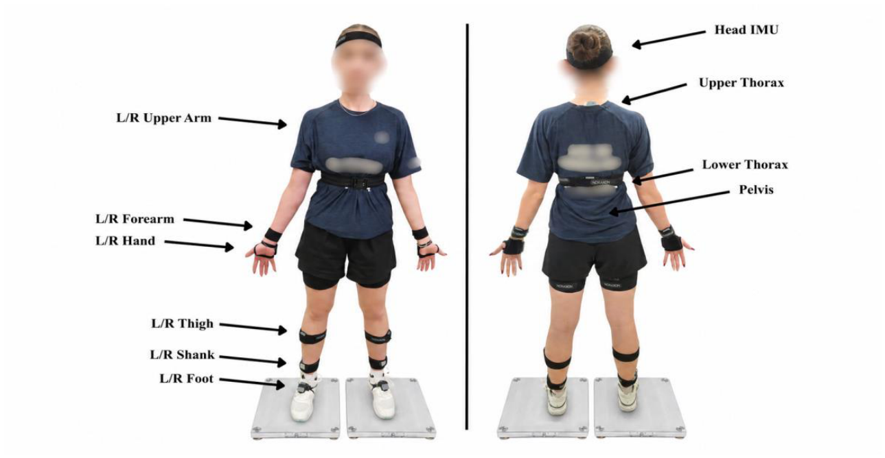
Figure 2.
Experimental equipment used for data collection: a table tennis table fitted with a ball-delivery robot and collection net, a video camera mounted on a tripod.
Figure 2.
Experimental equipment used for data collection: a table tennis table fitted with a ball-delivery robot and collection net, a video camera mounted on a tripod.
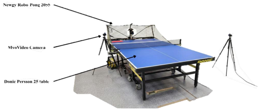
Figure 3.
Mean three-dimensional torso angular trajectories relative to the pelvis during cross-court (CC) and long-line (LL) strokes across the normalised movement cycle for the counter-topspin forehand (F_FH; top row), forehand topspin (TP_FH; middle row), and backhand topspin (TP_BH; bottom row). Flexion–extension is shown in the left column, lateral bending in the middle column, and axial rotation in the right column. Solid lines represent condition means and shaded envelopes represent ±1 standard deviation. The movement cycle was divided into backswing, forward-swing, and follow-through phases. Shaded red regions indicate significant CC–LL differences identified by one-dimensional statistical parametric mapping, with the corresponding cluster-level p-value shown in the panel.
Figure 3.
Mean three-dimensional torso angular trajectories relative to the pelvis during cross-court (CC) and long-line (LL) strokes across the normalised movement cycle for the counter-topspin forehand (F_FH; top row), forehand topspin (TP_FH; middle row), and backhand topspin (TP_BH; bottom row). Flexion–extension is shown in the left column, lateral bending in the middle column, and axial rotation in the right column. Solid lines represent condition means and shaded envelopes represent ±1 standard deviation. The movement cycle was divided into backswing, forward-swing, and follow-through phases. Shaded red regions indicate significant CC–LL differences identified by one-dimensional statistical parametric mapping, with the corresponding cluster-level p-value shown in the panel.
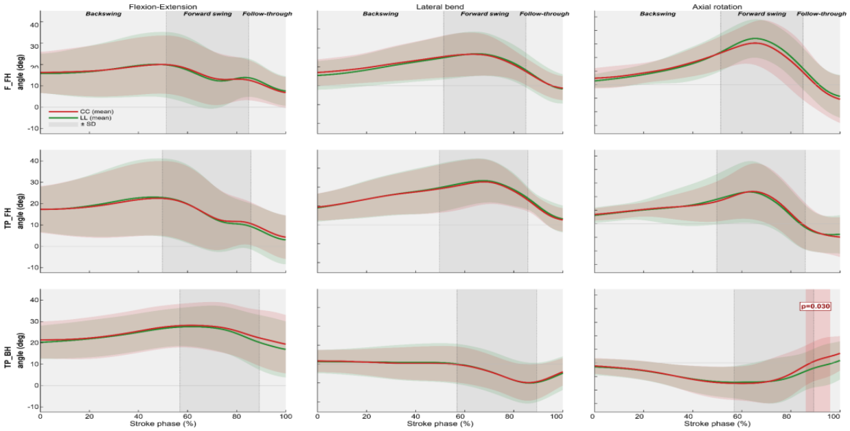

Table 1.
Within-subject differences between cross-court and long-line strokes for discrete kinematic variables. Positive CC − LL values indicate higher values in CC, whereas negative values indicate higher values in LL. SE, standard error; CI, confidence interval; d, Cohen’s effect size; FDR, false discovery rate.
Table 1.
Within-subject differences between cross-court and long-line strokes for discrete kinematic variables. Positive CC − LL values indicate higher values in CC, whereas negative values indicate higher values in LL. SE, standard error; CI, confidence interval; d, Cohen’s effect size; FDR, false discovery rate.
| Variable / Stroke | CC − LL | SE | Lower 95% CI | Upper 95% CI | d | p | p (FDR) |
|---|---|---|---|---|---|---|---|
| AR_contact | |||||||
| F_FH | -1.73 | 0.45 | -2.61 | -0.85 | -0.20 | 0.000 | 0.000 |
| TP_BH | 2.16 | 0.62 | 0.94 | 3.38 | 0.27 | 0.001 | 0.001 |
| TP_FH | 0.18 | 0.47 | -0.75 | 1.11 | 0.02 | 0.704 | 0.704 |
| FE_contact | |||||||
| F_FH | -0.56 | 0.36 | -1.28 | 0.15 | -0.06 | 0.123 | 0.123 |
| TP_BH | 2.51 | 0.49 | 1.54 | 3.48 | 0.19 | 0.000 | 0.000 |
| TP_FH | 1.42 | 0.43 | 0.58 | 2.27 | 0.13 | 0.001 | 0.002 |
| LB_contact | |||||||
| F_FH | -0.66 | 0.42 | -1.49 | 0.17 | -0.07 | 0.118 | 0.177 |
| TP_BH | 0.50 | 0.62 | -0.73 | 1.72 | 0.05 | 0.424 | 0.424 |
| TP_FH | -1.54 | 0.36 | -2.24 | -0.83 | -0.20 | 0.000 | 0.000 |
| ROM_AR | |||||||
| F_FH | 0.64 | 0.40 | -0.14 | 1.43 | 0.14 | 0.108 | 0.210 |
| TP_BH | 0.86 | 0.58 | -0.29 | 2.01 | 0.14 | 0.140 | 0.210 |
| TP_FH | 0.08 | 0.36 | -0.63 | 0.78 | 0.01 | 0.831 | 0.831 |
| ROM_FE | |||||||
| F_FH | -0.89 | 0.42 | -1.72 | -0.06 | -0.15 | 0.036 | 0.053 |
| TP_BH | -1.14 | 0.43 | -2.00 | -0.28 | -0.22 | 0.010 | 0.030 |
| TP_FH | -0.59 | 0.44 | -1.46 | 0.28 | -0.08 | 0.180 | 0.180 |
| ROM_LB | |||||||
| F_FH | 0.47 | 0.36 | -0.23 | 1.18 | 0.07 | 0.189 | 0.284 |
| TP_BH | 0.08 | 0.56 | -1.03 | 1.19 | 0.01 | 0.892 | 0.892 |
| TP_FH | 1.06 | 0.31 | 0.46 | 1.66 | 0.16 | 0.001 | 0.002 |
| XF_contact | |||||||
| F_FH | 2.13 | 0.49 | 1.16 | 3.10 | 0.27 | 0.000 | 0.000 |
| TP_BH | -2.78 | 0.86 | -4.47 | -1.08 | -0.33 | 0.002 | 0.002 |
| TP_FH | -0.48 | 0.49 | -1.44 | 0.48 | -0.06 | 0.327 | 0.327 |
| XF_max | |||||||
| F_FH | -0.89 | 0.41 | -1.70 | -0.08 | -0.09 | 0.031 | 0.093 |
| TP_BH | -0.19 | 0.52 | -1.21 | 0.83 | -0.03 | 0.712 | 0.712 |
| TP_FH | -0.25 | 0.30 | -0.84 | 0.34 | -0.02 | 0.408 | 0.612 |
| XF_stretch | |||||||
| F_FH | -0.37 | 0.45 | -1.26 | 0.53 | -0.09 | 0.422 | 0.422 |
| TP_BH | -0.36 | 0.38 | -1.11 | 0.39 | -0.06 | 0.344 | 0.422 |
| TP_FH | 0.76 | 0.24 | 0.29 | 1.23 | 0.28 | 0.002 | 0.005 |
| ωmax_AR | |||||||
| F_FH | 9.40 | 4.06 | 1.38 | 17.42 | 0.12 | 0.022 | 0.033 |
| TP_BH | 15.27 | 5.37 | 4.64 | 25.91 | 0.29 | 0.005 | 0.016 |
| TP_FH | -2.93 | 3.68 | -10.19 | 4.32 | -0.04 | 0.426 | 0.426 |
| ωmax_FE | |||||||
| F_FH | -3.67 | 3.29 | -10.17 | 2.82 | -0.06 | 0.266 | 0.266 |
| TP_BH | -7.46 | 3.94 | -15.25 | 0.33 | -0.14 | 0.060 | 0.099 |
| TP_FH | -6.75 | 3.65 | -13.96 | 0.46 | -0.10 | 0.066 | 0.099 |
| ωmax_LB | |||||||
| F_FH | 2.18 | 3.82 | -5.37 | 9.73 | 0.02 | 0.569 | 0.569 |
| TP_BH | 5.54 | 3.38 | -1.16 | 12.23 | 0.07 | 0.104 | 0.156 |
| TP_FH | 14.98 | 3.57 | 7.94 | 22.01 | 0.16 | 0.000 | 0.000 |
| ωmean_AR | |||||||
| F_FH | 3.50 | 2.35 | -1.15 | 8.14 | 0.11 | 0.139 | 0.139 |
| TP_BH | 6.31 | 2.93 | 0.51 | 12.12 | 0.20 | 0.033 | 0.057 |
| TP_FH | 4.21 | 2.01 | 0.24 | 8.19 | 0.10 | 0.038 | 0.057 |
| ωmean_FE | |||||||
| F_FH | -5.11 | 1.80 | -8.66 | -1.56 | -0.16 | 0.005 | 0.015 |
| TP_BH | -3.87 | 1.99 | -7.80 | 0.07 | -0.13 | 0.054 | 0.081 |
| TP_FH | -2.51 | 1.97 | -6.39 | 1.37 | -0.07 | 0.203 | 0.203 |
| ωmean_LB | |||||||
| F_FH | 0.42 | 1.69 | -2.92 | 3.76 | 0.01 | 0.805 | 0.805 |
| TP_BH | 2.56 | 2.47 | -2.33 | 7.45 | 0.05 | 0.302 | 0.453 |
| TP_FH | 5.80 | 1.46 | 2.91 | 8.69 | 0.16 | 0.000 | 0.000 |
* Notes: Values are estimated marginal mean differences (CC − LL) from linear mixed-effects models. Degrees of freedom were estimated using the Kenward–Roger method. Rows with p (FDR) < 0.05 are shown in bold. FDR correction was applied separately within each biomechanical indicator across the three stroke-technique contrasts. AR, axial rotation; FE, flexion–extension; LB, lateral bending; ROM, range of motion; XF, thorax–pelvis separation angle; ωmax, maximum angular velocity; ωmean, mean angular velocity; F_FH, forehand counter-topspin; TP_BH, backhand topspin; TP_FH, forehand topspin.
Disclaimer/Publisher’s Note: The statements, opinions and data contained in all publications are solely those of the individual author(s) and contributor(s) and not of MDPI and/or the editor(s). MDPI and/or the editor(s) disclaim responsibility for any injury to people or property resulting from any ideas, methods, instructions or products referred to in the content. |
© 2026 by the authors. Licensee MDPI, Basel, Switzerland. This article is an open access article distributed under the terms and conditions of the Creative Commons Attribution (CC BY) license (http://creativecommons.org/licenses/by/4.0/).
Copyright: This open access article is published under a Creative Commons CC BY 4.0 license, which permit the free download, distribution, and reuse, provided that the author and preprint are cited in any reuse.