

Submitted:
06 October 2026
Posted:
09 October 2026
You are already at the latest version
Abstract
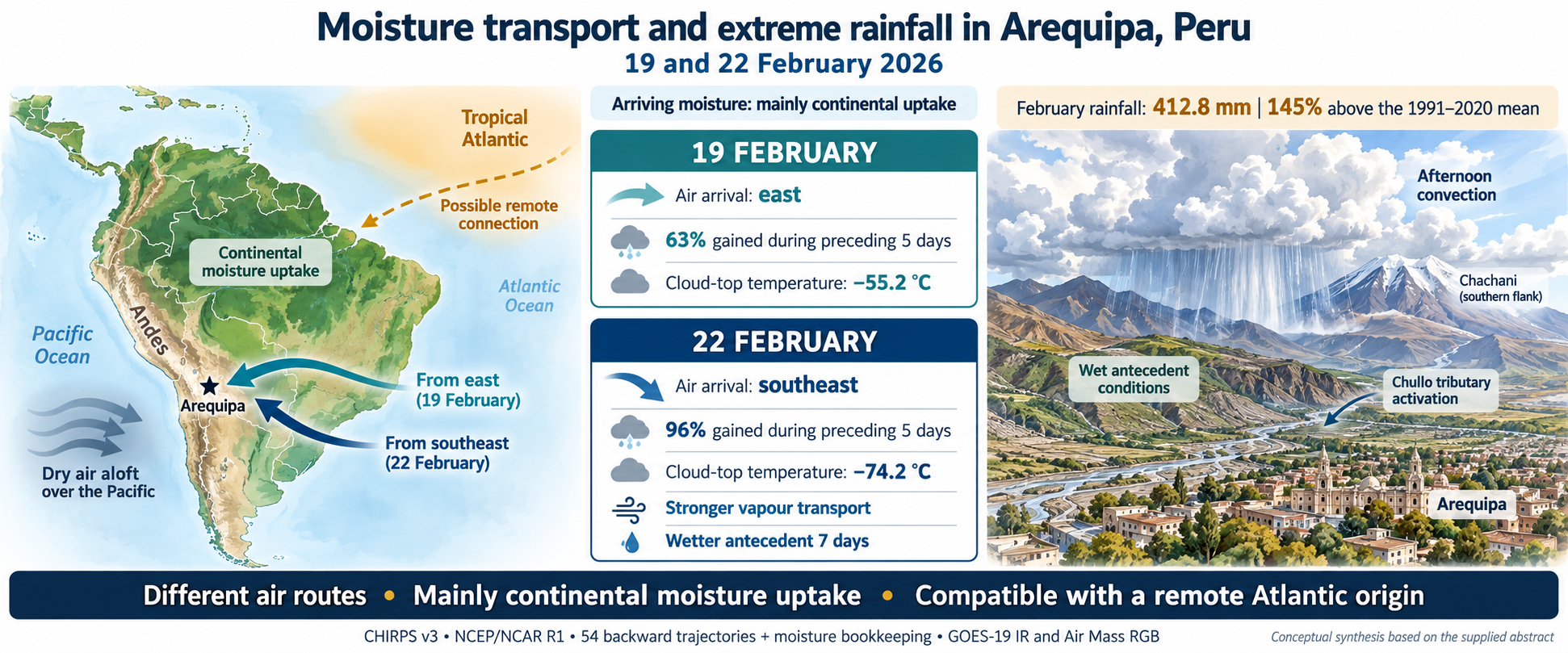
Ephemeral channels in Arequipa (Peru) convey floods and lahars during the rainy season. On 19 and 22 February 2026, tributaries of the Chullo channel on Chachani volcano’s southern flank became active, but the origin of the triggering rainfall was unknown. This study characterises both episodes from the continental to the local scale and assesses whether they shared a common moisture origin. We combined CHIRPS v3 precipitation, NCEP/NCAR R1 reanalysis, 54 backward trajectories with moisture bookkeeping, GOES-19 infrared imagery and Air Mass RGB composites. February 2026 rainfall (412.8 mm) was 145% above the 1991–2020 mean, and seven-day antecedent rainfall was larger before 22 February. Air arrived from the east on 19 February and from the southeast on 22 February, yet in both episodes most arriving moisture (63% and 96%) was gained over the preceding five days along mainly continental paths. Air Mass imagery showed a continuous tropical air mass from the tropical Atlantic to the southern Andes and dry air aloft over the adjacent Pacific. The second episode had stronger vapour transport and colder cloud tops (−74.2 vs. −55.2 °C). The Chullo activation reflected afternoon convection over wet antecedent conditions, fed by continental moisture compatible with a remote Atlantic origin.
Keywords:
central Andes
; lahars
; antecedent rainfall
; backward trajectories
; water vapour transport
; deep convection
; tropical air mass
; CHIRPS v3
; GOES-19
1. Introduction
Summer precipitation in the central Andes depends on the transport of water vapour from the continental lowlands towards the cordillera. During the austral summer, the tropical air mass associated with the South American monsoon extends from the tropical Atlantic over Amazonia to the Altiplano; the Bolivian High and the easterly flow at mid and upper levels favour the arrival of this moist air at the Altiplano and the western slope, while diurnal heating and slope circulations organise afternoon convection [1,2,3,4,5]. East of the Andes, the South American low-level jet redistributes Amazonian moisture southwards and controls the availability of water vapour in the subtropics [6]. Thus, the rainfall of a given episode results from the combination of the large-scale vapour supply and the processes that convert it into precipitation over the terrain.
Arequipa extends over the piedmont of the Chachani, Misti and Pichu Pichu volcanoes. Its ephemeral channels (torrenteras) remain dry most of the year, but during the rainy season they convey floods and lahars that cross urban areas [7]. In February 2026, descending lahars caused damage in the city, and the Instituto Geofísico del Perú (IGP) documented the activation of the tributaries of the Chullo channel on the southern flank of Chachani during the episodes of 19 and 22 February [8]. Historical records for the city show that these flows are concentrated in February and that the rainfall capable of triggering them depends on storm intensity and duration, but also on the rainfall accumulated over the preceding 24 hours or days [9]. These episodes offer an opportunity to examine whether events that activate the same drainage system share the same atmospheric origin.
However, knowledge of the origin of the moisture that feeds precipitation in the central Andes derives mainly from climatological analyses focused on the Altiplano and the eastern slope [1,2,3,4,5,6], and recent syntheses of Andean hydroclimate mostly address its variability at subcontinental and seasonal scales [10]. Event-scale analysis on the western slope of southern Peru, where annual rainfall is scarce and concentrated in a few days, has received much less attention. In Arequipa, studies of floods and lahars have focused on hazard zoning, flow simulation, building vulnerability and damage assessment [7,8,9], without characterising the atmospheric origin of the triggering rainfall. Nor has it been assessed whether successive episodes that activate the same drainage system respond to the same moisture pathway, or what weight antecedent rainfall and convective organisation carry relative to the regional vapour supply. In addition, verifiable rain-gauge records on the slopes of Chachani are scarce, which forces the use of estimated products whose daily distribution depends on the disaggregation method [11,12].
During the 2026 summer, positive sea surface temperature anomalies were recorded in the tropical Atlantic [13], and the easterly flow that feeds the region connects the cordillera with the tropical lowlands. Climate indices make it possible to summarise these large-scale oceanic and atmospheric signals and to relate them to regional precipitation [14]. In the eastern Pacific, by contrast, canonical ENSO must be distinguished from the Coastal El Niño, whose anomalous warming is concentrated off the northern coast of Peru, where it produces its largest rainfall impacts [15]; therefore, a coastal anomaly of this type does not by itself explain extreme rainfall on the southern western slope. Consequently, it is relevant to examine whether both episodes received a direct and common Atlantic contribution, or whether their moisture was incorporated in other regions. Answering this question requires distinguishing the trajectory of the air from the provenance of the water that precipitates: an air mass may cross an ocean, lose moisture and be moistened again over the continent [16]. Lagrangian diagnostics address this distinction by accounting for moisture gains and losses along computed trajectories [17,18].
The general objective of this study is to characterise the atmospheric conditions associated with the episodes of 19 and 22 February 2026 that activated the tributaries of the Chullo channel on the southern flank of Chachani, and to determine whether both shared the same moisture origin. The specific objectives are: (i) to quantify the exceptionality of January and February 2026 precipitation relative to the 1991–2020 period; (ii) to identify the transport pathways of the air that reached mid-levels in each episode, the regions where it incorporated its moisture and the large-scale context in which they developed, in order to establish whether there was a direct Atlantic contribution common to both; and (iii) to compare the regional humidity, vapour transport and convergence, convective organisation and antecedent rainfall of both episodes, in order to identify the factors associated with the activation of the Chullo. As a methodological contribution, the study integrates these scales within a single framework and explicitly assesses the sensitivity of the results to the daily disaggregation of precipitation and to the trajectory horizon. The results show that both episodes, although they followed different pathways, were fed mainly by moisture incorporated over the continent, on the western edge of a tropical air mass connected with the tropical Atlantic, and that antecedent rainfall and the organisation of afternoon convection distinguished the activation of the Chullo.
2. Materials and Methods
2.1. Study Area
A local analysis was carried out over a window of 71.65–71.50° W and 16.35–16.20° S, covering the piedmont and southern slope of Chachani between about 2400 m and more than 4500 m a.s.l. (Figure 1 and Figure 2a). In this sector, the IGP identifies the tributaries of the Chullo channel, including Azufral Lari Tucos, Azufral Gamarra and Pastoraiz, and documents reductions in channel width towards the urban area [8]. The window contains nine 0.05° CHIRPS cells, centred at longitudes −71.625, −71.575 and −71.525° and latitudes −16.225, −16.275 and −16.325°. It was treated as a fixed unit of comparison rather than a delineated catchment; it also contains the core of maximum CHIRPS precipitation in February 2026 (Figure 2c), an aspect discussed in Section 4.3.
The backward trajectories start from three receptors (R1–R3) located on the slopes of Chachani, each over one of the three main ravines that originate on the volcano and that, during the studied episodes, fed the Chullo channel in the reach where damage was recorded [8]. The receptors are located between 2922 and 2968 m a.s.l., where the ravines descend from the volcanic edifice towards the piedmont, about 11 km upstream of the affected sector of the channel (Figure 1). This choice linked the atmospheric analysis to the channels that were actually activated. Their coordinates are R1 (−71.5400°; −16.2977°), R2 (−71.5318°; −16.2981°) and R3 (−71.5263°; −16.2980°), obtained from UTM zone 19S coordinates (WGS84). To characterise the regional environment, a domain of four NCEP nodes (70–67.5° W; 15–17.5° S) was used, located east of Chachani over the sector through which the easterly flow enters towards the western slope; as a sensitivity test, two alternative domains with the same latitudes are used: 72.5–70° W and 72.5–67.5° W.
2.2. Data
This study integrated observational data, satellite products and atmospheric reanalysis fields to characterise the meteorological conditions and precipitation regime of the analysed episodes, from the local to the continental scale.
Precipitation was evaluated using CHIRPS v3 (Climate Hazards Center InfraRed Precipitation with Stations) [11,12], employing both its monthly version, for the climatological and recent-period analysis, and its daily satellite (sat) and reanalysis (rnl) products. Regional-scale dynamic and thermodynamic conditions were characterised with the NCEP/NCAR R1 reanalysis [20], from which key variables were extracted at eight pressure levels. To track deep convective cloudiness at the sub-daily scale, brightness temperature images from channel 13 (thermal infrared, 10.3 µm) of the ABI sensor on board the GOES-19 satellite were used [21].
The large-scale context was examined qualitatively with the Air Mass RGB composite of the geostationary ring available in NASA Worldview [22], which integrates three-hourly images from several geostationary satellites. Over South America, the composite comes from the GOES-East ABI sensor and combines the 6.2 and 7.3 µm water vapour channels and the 9.6 and 10.3 µm infrared channels. In this composite, green tones identify tropical air masses; red and orange, dry air at mid and upper levels; blue and violet, cold air masses; and white, thick high cloud [23]. Images at 21:00 UTC (16:00 PET) on 19 and 22 February 2026 were analysed, the available time closest to the minimum brightness temperature recorded in each episode.
Finally, the oceanic context was complemented with the NOAA CPC sea surface temperature indices [13], while the Terrain Tiles and Natural Earth cartographic layers [19,24] were used as a physiographic and orographic base.
The products used, their spatio-temporal resolutions and the selected coverage periods are summarised in Table 1. Rain-gauge records from local stations were not used because they could not be verified (Section 4.3).
2.3. Monthly Anomalies and Antecedent Precipitation
For each month, the arithmetic mean of the nine cells was calculated and compared with the 1991–2020 series for the same window. The percentage anomaly is defined as
where:
A = 100 (P2026 / Pref − 1)
Pref is the 1991–2020 mean.
The maximum of the reference period and the number of years exceeded are also reported; this empirical position is not interpreted as a return period. For each episode, precipitation over the seven complete preceding days is summed and, as a sensitivity test, over the three preceding days, excluding the day of the event. All daily calculations are repeated with sat and rnl.
2.4. Vapour Transport and Regional Convergence
The integrated vapour transport (IVT) and column precipitable water (W) are calculated between the surface pressure ps and 300 hPa:
with g = 9.80665 m s−2 and trapezoidal integration; levels below the model surface are excluded and the incomplete lowest layer is represented by the level immediately above. Transport convergence is obtained by centred finite differences on the spherical grid:
where:
IVT = (1/g) ∫300ps q v dp; W = (1/g) ∫300ps q dp
C = −86 400 [∂IVTλ/∂λ + ∂ (IVTφ cos φ) /∂φ] / (a cos φ)
λ and φ are longitude and latitude in radians,
a = 6.371 × 10⁶ m and the factor 86 400 expresses C in mm d−1;
Positive values indicate convergence. Regional averages are weighted by cos φ. Also calculated are ω at 500 hPa (negative values indicate ascent) and the spatial mean of q·u, which preserves the covariation between humidity and wind. Event maps average 18 UTC on the indicated day and 00 UTC on the following day. Given the truncation at 300 hPa and the reanalysis resolution, C is interpreted as a transport diagnostic and not as an estimate of P − E.
2.5. Backward Trajectories and Moisture Accounting
Trajectories were computed with the NCEP/NCAR R1 reanalysis because the aim is to identify synoptic-scale transport pathways, thousands of kilometres long, which a 2.5° grid resolves adequately; this reanalysis has been widely used to characterise moisture transport over South America [6]. Because the Andean relief is strongly smoothed in R1, arrivals were set in the mid-troposphere (450–550 hPa), above the model surface. The diagnostic characterises the mid-level air that feeds convection over Chachani and not the boundary-layer contribution, whose assessment requires a higher-resolution reanalysis (Section 4.4).
For each episode, 27 backward trajectories were integrated: three receptors, three arrival pressures (450, 500 and 550 hPa) and three arrival times (18 and 21 UTC on the event day and 00 UTC on the following day). The fields were linearly interpolated in time, pressure, latitude and longitude, and integrated with a fourth-order Runge–Kutta scheme, a 15 min time step and a maximum horizon of ten days:
dλ/dt = u / (a cos φ); dφ/dt = v / a; dp/dt = ω
Integration stops upon completing ten days, leaving the 85–25° W and 35° S–15° N domain, rising above 300 hPa, crossing the model surface or lacking interpolation data. Numerical robustness is checked by repeating the integration with a 30 min time step. Segments over the ocean are identified with the Natural Earth land mask [24] and labelled as Atlantic east of 60° W and as Pacific west of 65° W. Because the receptors are less than 1.5 km apart (far below the 2.5° grid spacing), the ensemble is in practice equivalent to nine combinations of arrival level and time; member counts are interpreted in this sense. The position error of trajectories computed from reanalysis grows with integration time and is typically around 10–20% of the distance travelled [25], so the oldest segments are the least reliable.
To quantify where moisture is incorporated, q is sampled every six hours from the oldest point to arrival, following the sequential accounting of gains and losses used in Lagrangian diagnostics [17,18]. Each increase in q is recorded as a new contribution; upon a decrease, all previous contributions are reduced proportionally:
where:
Mj,n = Mj,n−1 · qn / qn−1 if Δqn < 0
Mj,n is the moisture of contribution j retained at time step n.
Arrival moisture is decomposed into a fraction present at the start of the window and a fraction incorporated during transport. Because the trajectories do not parameterise turbulent mixing or convection, increases in q are termed net moisture increments and are not directly identified with surface evaporation; only increments occurring with the parcel near the model surface (p/ps ≥ 0.8) would be considered of possible surface origin. Five-day results include all members; ten-day results include only complete trajectories.
2.6. Cloud Tops
ABI scan angles are transformed into geographic coordinates using the projection parameters of each file, and pixels whose centre falls within the window are selected, retaining only values with quality flag DQF = 0 (64 pixels per scene). For each scene, the minimum brightness temperature and the fraction of pixels below −40, −50 and −60 °C are calculated. Brightness temperature characterises the height and extent of convective tops and is not converted into rainfall intensity.
2.7. Large-Scale Context
The Air Mass images of 19 and 22 February at 21:00 UTC were interpreted visually over a domain between 10° N and 40° S and between 90° and 30° W, covering the tropical Atlantic, South America and the southeastern Pacific. The extent of the tropical air mass, the presence of dry air aloft, the distribution of deep convection and the main synoptic systems (ITCZ, subtropical convective systems and South Atlantic cyclones) were identified. The analysis is qualitative and was used to place the trajectories and local convection in their continental context.
3. Results
Results are presented from the monthly to the sub-daily scale. Section 3.1 addresses the first objective; Section 3.4 and Section 3.5, the second; and Section 3.2, Section 3.3 and Section 3.6 bring together the elements of the third.
3.1. Exceptionality of Monthly Precipitation
February 2026 accumulated 412.79 mm in the window, 145.4% above the 1991–2020 mean and 80.6 mm (24.3%) above the maximum of the thirty reference Februaries (Table 2; Figure 3a).
January accumulated 87.29 mm, 117.3% above its mean; it exceeded 29 of the 30 reference Januaries and remained below the maximum of 96.85 mm. The exceptional character is therefore concentrated in February, although it was preceded by a January that was also wet.
3.2. Precipitation During the Episodes and Antecedent Accumulation
The daily disaggregations sat and rnl preserve the same February 2026 monthly total but differ in its temporal distribution (Figure 3b). These differences reverse the comparison between the episodes: with sat, precipitation on 19 February (20.89 mm) exceeds that on 22 February (14.52 mm), whereas with rnl the total on 22 February (20.89 mm) is larger than on 19 February (15.74 mm; Table 3).
In contrast, both disaggregations show greater accumulated precipitation over the seven days before the 22 February episode. In sat, this accumulation increases from 102.47 to 199.97 mm between the two episodes; in rnl, from 144.73 to 170.21 mm. Days 20 and 21 together contribute 106.0 mm in sat and 51.6 mm in rnl to the accumulation before 22 February, although the difference between the seven-day windows also depends on the other days they comprise.
For the three preceding days, the comparison again depends on the disaggregation: sat shows greater accumulation before 22 February, whereas rnl places it before 19 February. Therefore, the result consistent between both disaggregations is the greater seven-day antecedent accumulation before the 22 February episode; this agreement does not hold for the three-day window or for precipitation on the day of the episode itself.
3.3. Regional Circulation and Moisture Transport Convergence
Figure 4 shows the regional distribution of moisture and atmospheric circulation during the episodes of 19 and 22 February 2026. The upper panels show specific humidity and wind at 500 hPa; the lower panels show the convergence of integrated vapour transport and the transport vectors. Each map corresponds to the average of 13:00 and 19:00 Peru time (PET; UTC−5), so it describes the mean conditions of both times and not their evolution within that interval.
On 19 February, the highest 500 hPa humidity values are observed over Amazonia, with an additional core over interior Brazil (Figure 4a). On 22 February, a more extensive moist band stands out east of the Andes, from eastern Bolivia towards central and southeastern Brazil, with values above 3 g kg−1 over large areas (Figure 4b). This band does not extend with the same magnitude to Arequipa: both the area marked by the star and the domain delimited by the box show lower humidity than the continental cores. Nevertheless, Table 4 confirms that the mean humidity of the domain was higher on 22 February than on 19 February, by approximately 34% at 13:00 and 40% at 19:00.
The 500 hPa wind had an easterly component (westward motion, indicated by u < 0) in all four records analysed. On 19 February, this component reached −6.54 m s−1 at both times. On 22 February it was weak at 13:00 (−0.94 m s−1) and strengthened towards 19:00 (−4.94 m s−1). Consequently, the higher humidity on 22 February was not accompanied by greater zonal transport at all times: the spatial mean of q·u was much smaller in magnitude at 13:00 than on 19 February, whereas at 19:00 it was similar in both episodes.
The lower panels show a heterogeneous distribution of convergence and divergence of vapour transport. Green tones indicate convergence, that is, net vapour inflow by horizontal transport; brown tones indicate divergence or net outflow. On 22 February, an extensive area of convergence is seen east of the Andes, over parts of Bolivia and Brazil (Figure 4d). However, the surroundings of Arequipa and the regional box lie close to a transition between both signs. Therefore, the convergence of the continental cores should not be attributed directly to the El Chullo catchment.
The hourly evolution in Table 4 complements this spatial distribution. In the selected domain, both episodes changed from divergence at 13:00 to convergence at 19:00. At 19:00 on 22 February, the largest integrated vapour transport of the four times evaluated was recorded (97.6 kg m−1 s−1), accompanied by mean ascent at 500 hPa (ω = −0.054 Pa s−1). On 19 February at the same time, transport was lower (36.9 kg m−1 s−1) and vertical motion was close to zero (ω = +0.004 Pa s−1), although convergence was greater: +5.30 versus +3.63 mm d−1.
Convergence at 19:00 remained positive in the three domains evaluated for both episodes, whereas at 13:00 on 22 February its sign depended on the domain. Overall, the results show that the second episode presented, at 19:00, a combination of higher humidity, greater integrated vapour transport and regional ascent. These conditions characterise an environment favourable for the development of precipitation, but their relationship with rainfall over the El Chullo contributing catchment must be established through local observations with higher temporal resolution.
3.4. Large-Scale Context During the Episodes
The Air Mass images at 21:00 UTC (16:00 PET) show, in both episodes, a continuous tropical air mass extending from the tropical Atlantic over Amazonia and Bolivia to the eastern slope of the southern Andes, with abundant deep convection in the interior of the continent (Figure 5). West of the cordillera, over the southeastern Pacific off southern Peru and northern Chile, dark olive and brownish tones associated with dry air at mid and upper levels predominate, with no deep convection over the ocean. The ITCZ appears as an independent band north of the equator, with no cloud continuity with southern Peru.
The two episodes differ in the organisation of convection. On 19 February (Figure 5a), Arequipa lies on the western edge of the tropical air mass, continental convection is more scattered, and two compact convective cores stand out over Paraguay and northern Argentina, together with a mature extratropical cyclone over the South Atlantic. On 22 February (Figure 5b), convection is more extensive and organised over western Amazonia and Bolivia, and reaches the Andean edge immediately east of Arequipa at the time of the event; over the South Atlantic, the cyclonic system appears less defined.
3.5. Atmospheric Pathways and Moisture Incorporation
The backward trajectories show differences in the pathways of the air that reached the receptors during the two episodes (Figure 6). Colour represents the time before arrival: violet segments correspond to the most recent part of the path and yellow segments to approximately ten days earlier.
On 19 February, all 27 trajectories completed ten days of backward tracking. In their final segment, the air arrived from the east along an approximately zonal path around 16° S. Earlier segments show broad recurvatures over south-central and southeastern Brazil, with incursions over the Atlantic in part of the oldest segment. On 22 February, the trajectories arrived from the southeast, after crossing parts of Bolivia, Paraguay and northern Argentina. Further back in time, they extended over Argentina and Chile to the subtropical Pacific, without reaching the Atlantic within the computed interval. These pathways describe the history of air motion and do not, by themselves, identify the origin of the vapour the air contained on arrival.
The temporal coverage of the ensemble differed between episodes. All trajectories for 22 February completed five days, but only nine reached ten days: six were interrupted on crossing the western boundary of the domain and twelve on reaching levels with pressure below 300 hPa, outside the vertical integration range. The interrupted trajectories spanned between 5.5 and 8.5 days. Therefore, the five-day horizon allows the 27 members of each episode to be compared, whereas the ten-day horizon represents only a subset for 22 February.
The decomposition of arrival specific humidity distinguishes the moisture present at the start of each horizon that remains until the receptor from the increments acquired along the path that are also retained until arrival (Table 5). At five days, these retained increments represent 63.2% of arrival moisture on 19 February and 95.9% on 22 February. The results indicate a greater contribution of recent moistening in the second episode.
During those five days, the pathways ran mainly over South America. This places much of the recent path in a continental environment. Quantifying this contribution requires locating the retained increments and distinguishing the processes that produce them. Moreover, the percentages in Table 5 refer to the specific humidity of the parcels on arrival, not directly to fractions of the observed precipitation.
For the ten-day horizon, retained initial moisture represents 18.5% in the full ensemble for 19 February and 1.4% in the nine complete members for 22 February; retained increments represent 81.5% and 98.6%, respectively. The comparison between horizons for 22 February is conditioned by the change in sample. To separate this effect from that associated with tracking duration, the five- and ten-day results should also be compared for those same nine members.
Sensitivity to the time step was assessed by repeating the integration with 30 min intervals, compared with 15 min in the main calculation. The maximum horizontal separation between the terminal backward positions was 0.09 km at five days and 2.86 km at ten days; in the latter case, the 36 complete pairs from both episodes were compared. Pressure differences were 0.02 and 0.13 hPa, respectively. These results show low sensitivity to the time step tested, but do not quantify the trajectory uncertainty associated with the reanalysis, its spatial resolution or the representation of atmospheric motions.
3.6. Evolution and Extent of Cold Cloud Tops
GOES-19 channel 13 observations show cloudiness with colder tops and greater coverage of low temperatures during the afternoon of 22 February than during that of 19 February (Figure 7). The comparison was made over a 64-pixel window, using the minimum brightness temperature and the percentage of pixels with temperatures below −40 and −60 °C.
On 19 February, the minimum temperature in the window reached −55.2 °C at 17:00 Peru time (PET; UTC−5). At that time, 23.4% of pixels had temperatures below −40 °C, while none fell below −60 °C. The lowest temperatures within the window were located in its southern sector; the surrounding scene also shows cold cloudiness south of the box.
On 22 February, the decrease in minimum temperature intensified from 14:00 onwards and reached −74.2 °C at 16:00, a minimum 19.0 °C lower than that of the 19 February episode. At that time, 90.6% of pixels had temperatures below −60 °C. Moreover, in the three observations at 15:00, 16:00 and 17:00, 100% of pixels were below −40 °C. These results show that cold-topped cloudiness covered a larger proportion of the window and was present in more consecutive hourly samples during the second episode.
The contrast is compatible with greater vertical development of cloudiness on 22 February. However, brightness temperature is an indirect indicator of cloud-top characteristics and cannot by itself quantify surface precipitation. Furthermore, since the images are not parallax-corrected, the apparent location of the tops should be interpreted with caution when relating it to specific sectors of the contributing catchment.
4. Discussion
4.1. Air Pathway and Moisture Origin
The episodes had different arrival pathways: from the east on 19 February, consistent with summertime transport towards the central Andes [1,2,3,4,5], and from the southeast on 22 February, after a subtropical path. Despite this, the moisture increments retained during the preceding five days represented 63.2% and 95.9% of arrival moisture, respectively. The mainly continental transit during that interval is compatible with moistening and recycling processes over South America [16], although it does not allow all increments to be attributed to terrestrial evapotranspiration. The diagnostic refers to parcels arriving at mid-levels and does not directly assess the contribution of the low-level jet.
The trajectories do not demonstrate a common direct Atlantic contribution; contact with the Atlantic appears only in old segments of the 19 February episode, whereas the 22 February episode includes paths over the subtropical Pacific. However, crossing an ocean does not demonstrate moisture uptake from its surface, and the retained initial fractions in Table 5 are not equivalent to oceanic contributions. The reconstruction for 22 February is further limited by the interruption of 18 trajectories before ten days. Therefore, the results support the importance of recent moistening, but quantifying the remote oceanic origin and continental recycling requires an additional source diagnostic.
The large-scale context complements this result. In both episodes, the convection that affected the southern flank of Chachani developed on the western edge of a tropical air mass that extended uninterrupted from the tropical Atlantic over Amazonia and Bolivia, while the Pacific off the southern coast showed dry air aloft and an absence of deep convection (Figure 5). This pattern is compatible with an indirect Atlantic contribution, mediated by moisture recycling over Amazonia, whose main oceanic source is the tropical Atlantic [26], and does not support a local supply from the Pacific.
4.2. Antecedent Rainfall, Convection and Activation of the Chullo Channel
Regarding the third objective, the comparison of daily rainfall between episodes is inconclusive, because it depends on how the same pentadal total is distributed among days [12]. The robust differences between the two episodes lie elsewhere: 22 February combined higher regional humidity, greater vapour transport with late-afternoon ascent, colder and more extensive cloud tops, and a larger seven-day accumulation in both disaggregations, concentrated on 20 and 21 February. This combination describes a more organised convective episode that developed over a system already moistened by rainfall on the preceding days.
The Air Mass images reinforce this contrast: on 22 February, continental convection was more extensive and organised and reached the Andean edge east of Arequipa at the time of the event (Figure 5).
The activation mechanism of the Chullo can be described by distinguishing the meteorological trigger from the drainage conditioning factors. Afternoon convection delivers intense rainfall over the slope within a few hours; the volcanic relief concentrates runoff in the tributaries identified by the IGP [8]; and sediment availability and channel constrictions towards the city have favoured the transformation of floods into sediment-laden flows, as documented for the ephemeral channels of Arequipa [7,9]. Antecedent rainfall reduces soil storage capacity and can accelerate the response, although its effect depends on infiltration and the state of the channel.
From an early-warning perspective, the results suggest that the combination of high seven-day accumulations with cold and extensive convective tops over the southern flank constitutes a signal that can be monitored in near real time.
4.3. Uncertainty of the Estimated Precipitation
CHIRPS magnitudes should be interpreted as product estimates. First, the window contains the core of maximum February precipitation (Figure 2c), so its anomaly represents the wettest sector of the product and not the whole catchment. Comparison with each cell’s own climatology mitigates this effect but does not eliminate it. Second, CHIRPS v3 incorporates stations and an undercatch correction [11], and it was not possible to determine which stations contributed to the estimate for this area in February 2026. Third, the available rain-gauge records could not be verified and were not used (Section 2.2). For these reasons, the conclusions rely on robust internal features of the product (the position of February relative to its climatology and the ranking of seven-day accumulation between episodes) and not on absolute values for a specific day. An independent evaluation with PISCOp [27], the national product that combines SENAMHI rain gauges with satellite estimates, would help constrain these magnitudes.
4.4. Limitations and Perspectives
The NCEP/NCAR R1 reanalysis, with a 2.5° grid and humidity up to 300 hPa, resolves the synoptic circulation but represents Andean relief in a simplified way and does not resolve slope flows or convective cells. Arrivals at 450–550 hPa do not sample the boundary layer; therefore, none of the moisture increments met the surface-proximity criterion (p/ps ≥ 0.8), and the accounting describes moistening in the free troposphere, compatible with mixing and convective transport from lower layers. The GOES images were not corrected for parallax, which can shift the apparent position of the tops by a few kilometres, and hourly sampling does not guarantee capturing the absolute minimum of each storm.
This study did not include trajectories computed with ERA5 [28]. Therefore, the conclusions on moisture origin refer to air arriving at mid-levels and do not quantify the fraction taken up from the surface or its partition between the continent and the oceans. Three extensions would strengthen these conclusions: (i) repeating the trajectories with ERA5, at hourly and 0.25° resolution, including arrivals in the boundary layer and an uptake criterion based on its diagnosed height, which is the priority extension of this work; (ii) delineating the Chullo catchment with a high-resolution digital elevation model and calculating areal precipitation over it; and (iii) comparing CHIRPS with PISCOp and IMERG Final and, when available, with official hourly SENAMHI series.
The characterisation of the large-scale context was based on three-hourly images of the Air Mass composite, which describe air masses and cloudiness at mid and upper levels, but not moisture transport in the boundary layer or its temporal evolution. A quantitative analysis of continental vapour transport, the position of the Bolivian High and remote sources using Lagrangian models with a longer horizon would allow the contribution of the tropical Atlantic to be determined more precisely.
Likewise, GRACE/GRACE-FO satellite gravimetry, which has made it possible to characterise groundwater storage variability in Peru [29], could be used to assess, at the regional scale, the hydrological response of the western slope to the exceptional rainfall of February 2026.
5. Conclusions
With regard to the stated objectives, the results support the following conclusions:
- -
- February 2026 was exceptional on the southern flank of Chachani according to CHIRPS v3: it accumulated 412.8 mm, 145% above the 1991–2020 mean and 24% above the maximum of that period, after a January that exceeded 29 of its 30 reference years.
- -
- The episodes of 19 and 22 February followed different atmospheric pathways: the first from the east across Brazil; the second from the southeast after recurving over Argentina. They did not share a common oceanic pathway, and the Atlantic contact on 19 February is limited to the oldest and most uncertain segment of the trajectories.
- -
- According to the trajectories computed with NCEP/NCAR R1, in both episodes most of the moisture that reached mid-levels (63% and 96% within five days) was incorporated during transport over the continent. Continental moistening, rather than a direct oceanic contribution, explains the vapour supply in the mid-troposphere in both events, without excluding a remote Atlantic origin of that moisture; the boundary-layer contribution remains to be assessed with a higher-resolution reanalysis.
- -
- The Air Mass images show that, in both episodes, convection over the southern flank of Chachani developed on the western edge of a tropical air mass continuous from the tropical Atlantic to the southern Andes, while the Pacific off the coast showed dry air aloft. This context is compatible with a remote Atlantic origin of the moisture, incorporated and recycled over Amazonia.
- -
- The 22 February episode combined higher regional humidity, greater vapour transport with late-afternoon ascent, colder cloud tops (minimum of −74.2 °C, with the whole window below −40 °C for three hours) and a larger seven-day accumulation in both disaggregations. The ranking of daily rainfall between episodes, by contrast, depends on the disaggregation and is inconclusive.
- -
- The activation of the Chullo channel was associated with afternoon convection over a system with exceptional antecedent rainfall, concentrated by the relief of the southern flank and, according to the available geomorphological evidence, conditioned by sediment and channel constrictions. Joint monitoring of seven-day accumulated rainfall and of the extent of cold tops over the southern flank could support early warning of these events.
Author Contributions
Conceptualization, E.G.; methodology, E.G.; software, E.G. and S.G.; validation, E.G.; formal analysis, E.G. and S.G.; investigation, E.G.; writing—review and editing, E.G.; visualization, E.G. and S.G. All authors have read and agreed to the published version of the manuscript.
Funding
This research received no external funding.
Data Availability Statement
The data presented in this study were derived from the following resources available in the public domain: CHIRPS v3 (Climate Hazards Center, University of California, Santa Barbara; https://data.chc.ucsb.edu/products/CHIRPS/v3.0/), NCEP/NCAR Reanalysis 1 (NOAA PSL; https://psl.noaa.gov/data/gridded/data.ncep.reanalysis.html), GOES-19 ABI data (NOAA, Registry of Open Data on AWS; https://registry.opendata.aws/noaa-goes/), the Air Mass composite of the geostationary ring (NASA Worldview/GIBS; https://worldview.earthdata.nasa.gov), NOAA CPC oceanic indices, Terrain Tiles and Natural Earth.
Acknowledgments
The authors thank the Climate Hazards Center, NOAA and the Registry of Open Data on AWS for open access to the data used. We acknowledge the use of imagery from the NASA Worldview application (https://worldview.earthdata.nasa.gov), part of the NASA Earth Observing System Data and Information System (EOSDIS). During the preparation of this manuscript, the authors used Claude (Anthropic, Claude Opus 5.5) for the purposes of revising the wording and translation, and ChatGPT (OpenAI, V6) to assist with image processing. The authors have reviewed and edited the output and take full responsibility for the content of this publication.
Conflicts of Interest
The authors declare no conflicts of interest.
References
- Garreaud, R. D. Multiscale analysis of the summertime precipitation over the central Andes. Mon. Weather Rev. 1999, 127, 901–921. [Google Scholar] [CrossRef]
- Garreaud, R. D. Intraseasonal variability of moisture and rainfall over the South American Altiplano. Mon. Weather Rev. 2000, 128, 3337–3346. [Google Scholar] [CrossRef]
- Garreaud, R.; Vuille, M.; Clement, A. C. The climate of the Altiplano: observed current conditions and mechanisms of past changes. Palaeogeogr. Palaeoclimatol. Palaeoecol. 2003, 194, 5–22. Available online: https://www.sciencedirect.com/science/article/abs/pii/S0031018203002694?via%3Dihub. [CrossRef]
- Lenters, J. D.; Cook, K. H. On the origin of the Bolivian High and related circulation features of the South American climate. J. Atmos. Sci. 1997, 54, 656–678. [Google Scholar] [CrossRef]
- Vuille, M. Atmospheric circulation over the Bolivian Altiplano during dry and wet periods and extreme phases of the Southern Oscillation. Int. J. Climatol. 1999, 19, 1579–1600. [Google Scholar] [CrossRef]
- Marengo, J. A.; Soares, W. R.; Saulo, C.; Nicolini, M. Climatology of the low-level jet east of the Andes as derived from the NCEP–NCAR reanalyses: characteristics and temporal variability. J. Clim. 2004, 17, 2261–2280. [Google Scholar] [CrossRef]
- Thouret, J.-C.; Enjolras, G.; Martelli, K.; Santoni, O.; Luque, J. A.; Nagata, M.; Arguedas, A.; Macedo, L. Combining criteria for delineating lahar- and flash-flood-prone hazard and risk zones for the city of Arequipa, Peru. Nat. Hazards Earth Syst. Sci. 2013, 13, 339–360. [Google Scholar] [CrossRef]
- Rivera, M.; Valdivia, D.; Cuno, J.; Arias, C.; Cruz, J.; Cuadros, B.; Cabrera, M. Evaluación geodinámica de los daños ocasionados por el descenso de lahares en la ciudad de Arequipa durante febrero de 2026 (Región Arequipa) [in Spanish]; Instituto Geofísico del Perú, 2026; Available online: https://repositorio.igp.gob.pe/server/api/core/bitstreams/a96bc6c3-f122-4ac1-bc64-2728c6424a83/content.
- Thouret, J.-C.; Arapa, E.; Charbonnier, S.; Guerrero, A.; Kelfoun, K.; Cordoba, G.; Rodriguez, D.; Santoni, O. Modeling tephra fall and sediment-water flows to assess their impacts on a vulnerable building stock in the city of Arequipa, Peru. Front. Earth Sci. 2022, 10, 865989. [Google Scholar] [CrossRef]
- Arias, P. A.; Garreaud, R.; Poveda, G.; Espinoza, J. C.; Molina-Carpio, J.; Masiokas, M.; Viale, M.; Scaff, L.; van Oevelen, P. J. Hydroclimate of the Andes Part II: Hydroclimate variability and sub-continental patterns. Front. Earth Sci. 2021, 8, 505467. [Google Scholar] [CrossRef]
- Funk, C.; Peterson, P.; Harrison, L.; Saldivar, R.; Landsfeld, M.; Pedreros, D.; Shukla, S.; Fink, A. H.; Davenport, F.; Peterson, S. H.; Turner, W.; Sonnier, A.; Budde, M.; Tabor, K.; Verdin, J.; Hauzaree, D.; Naim, M.; Alaso, D.; Husak, G. The Climate Hazards Center Infrared Precipitation with Stations, version 3. Sci. Data 2026, 13, 718. [Google Scholar] [CrossRef] [PubMed]
- Climate Hazards Center, University of California Santa Barbara. CHIRPS v3: daily product documentation. 2026. Available online: https://www.chc.ucsb.edu/data/chirps3.
- NOAA Climate Prediction Center. Climate Diagnostics Bulletin, February 2026, Table 2: Oceanic indices. 2026. Available online: https://www.cpc.ncep.noaa.gov/products/CDB/CDB_Archive_html/bulletin_022026/Tropics/table2.shtml.
- Gonzales, E.; Gonzales, K. Analysis of Climate Indices to Determine Global Climate Patterns: Techniques for Summarizing Complex Climate Data. In Climate Change and Risk Management-Strategies, Analysis, and Adaptation; IntechOpen, 2024. [Google Scholar] [CrossRef]
- Gonzales, E.; Ingol, E. Determination of a new coastal ENSO oceanic index for northern Peru. Climate 2021, 9(5), 71. [Google Scholar] [CrossRef]
- Gimeno, L.; Stohl, A.; Trigo, R. M.; Dominguez, F.; Yoshimura, K.; Yu, L.; Drumond, A.; Durán-Quesada, A. M.; Nieto, R. Oceanic and terrestrial sources of continental precipitation. Rev. Geophys. 2012, 50, RG4003. [Google Scholar] [CrossRef]
- Stohl, A.; James, P. A Lagrangian analysis of the atmospheric branch of the global water cycle. Part I: Method description, validation, and demonstration for the August 2002 flooding in central Europe. J. Hydrometeorol. 2004, 5, 656–678. [Google Scholar] [CrossRef]
- Sodemann, H.; Schwierz, C.; Wernli, H. Interannual variability of Greenland winter precipitation sources: Lagrangian moisture diagnostic and North Atlantic Oscillation influence. J. Geophys. Res. Atmos. 2008, 113, D03107. [Google Scholar] [CrossRef]
- Mapzen. Terrain Tiles (Terrarium), zoom 10. Registry of Open Data on AWS. Available online: https://registry.opendata.aws/terrain-tiles/.
- Kalnay, E.; Kanamitsu, M.; Kistler, R.; et al. The NCEP/NCAR 40-Year Reanalysis Project. Bull. Am. Meteorol. Soc. 1996, 77, 437–471. [Google Scholar] [CrossRef]
- Schmit, T. J.; Griffith, P.; Gunshor, M. M.; Daniels, J. M.; Goodman, S. J.; Lebair, W. J. A closer look at the ABI on the GOES-R series. Bull. Am. Meteorol. Soc. 2017, 98, 681–698. [Google Scholar] [CrossRef]
- NASA Worldview. Air Mass (Geostationary Ring, 3 hour). NASA Earth Observing System Data and Information System (EOSDIS), Global Imagery Browse Services (GIBS). Available online: https://worldview.earthdata.nasa.gov (accessed on 4 October 2026).
- Berndt, E. Quick Guide: Air Mass RGB. NASA Short-term Prediction Research and Transition Center (SPoRT) – NOAA GOES-R. Available online: https://goes.noaa.gov/documents/QuickGuide_GOESR_AirMassRGB_final.pdf.
- Natural Earth. Admin 0 – Countries, scale 1:110 million. Available online: https://www.naturalearthdata.com/.
- Stohl, A. Computation, accuracy and applications of trajectories—A review and bibliography. Atmos. Environ. 1998, 32, 947–966. [Google Scholar] [CrossRef]
- Drumond, A.; Marengo, J.; Ambrizzi, T.; Nieto, R.; Moreira, L.; Gimeno, L. The role of the Amazon Basin moisture in the atmospheric branch of the hydrological cycle: a Lagrangian analysis. Hydrol. Earth Syst. Sci. 2014, 18, 2577–2598. [Google Scholar] [CrossRef]
- Aybar, C.; Fernández, C.; Huerta, A.; Lavado, W.; Vega, F.; Felipe-Obando, O. Construction of a high-resolution gridded rainfall dataset for Peru from 1981 to the present day. Hydrol. Sci. J. 2020, 65, 770–785. [Google Scholar] [CrossRef]
- Hersbach, H.; Bell, B.; Berrisford, P.; et al. The ERA5 global reanalysis. Q. J. R. Meteorol. Soc. 2020, 146, 1999–2049. [Google Scholar] [CrossRef]
- Gonzales, E.; Alvarez, V.; Gonzales, K. Two Decades of Groundwater Variability in Peru Using Satellite Gravimetry Data. Appl. Sci. 2025, 15(14), 8071. [Google Scholar] [CrossRef]
Figure 1.
Location of the study area on the southern flank of Chachani volcano (Arequipa, Peru). The magenta rectangle delimits the CHIRPS window of nine 0.05° cells; yellow circles indicate receptors R1–R3, located over the three main tributary ravines of the Chullo channel (2922–2968 m), and the light-blue square marks the sector of the Chullo channel where damage was recorded. (Source: Google Earth; © 2026 Airbus).
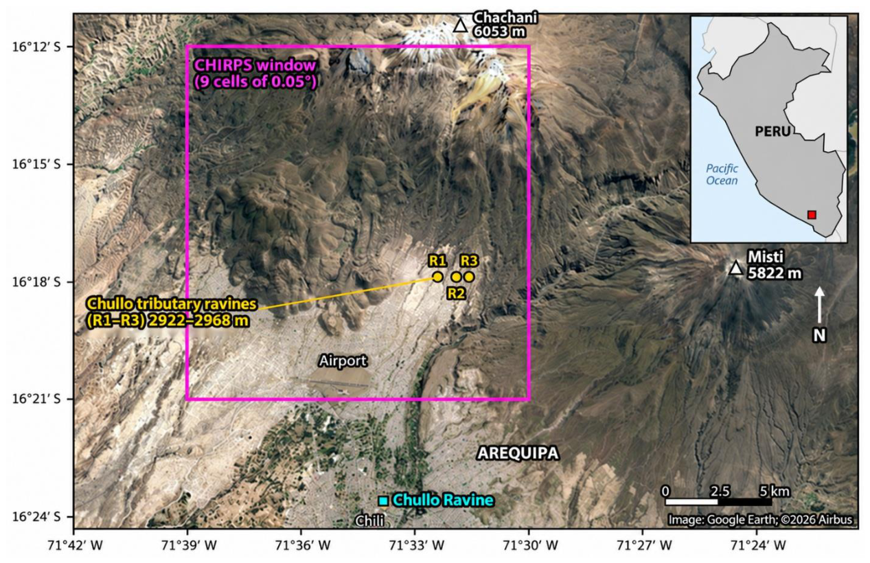
Figure 2.
(a) Relief of the study area and reference localities; the red rectangle delimits the nine-cell window and the blue crosses mark receptors R1–R3. (b, c) Monthly CHIRPS v3 precipitation in January and February 2026. (Relief: Terrain Tiles digital elevation model, zoom level 10, approximate resolution 150 m [19]). The figure does not represent catchment divides.
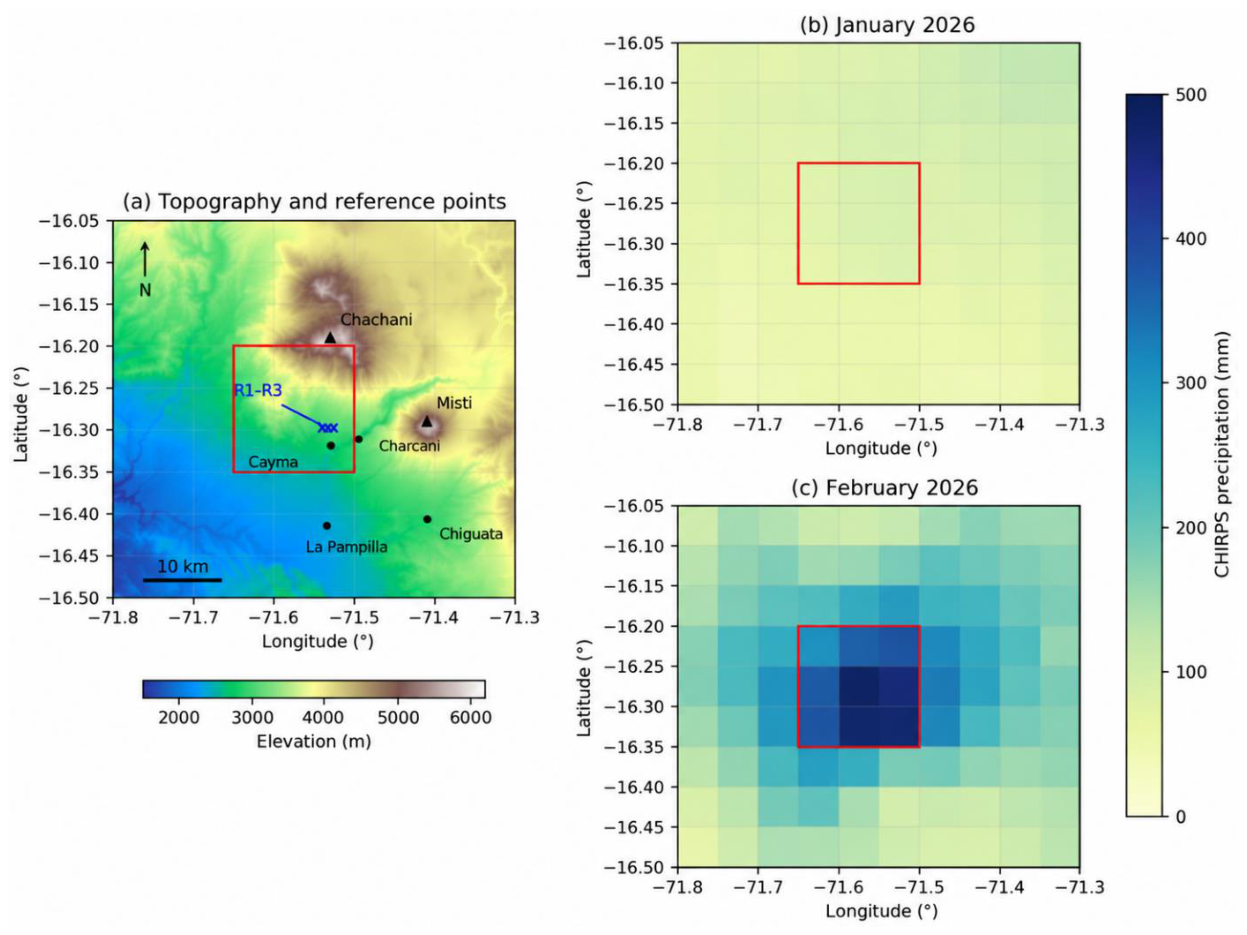
Figure 3.
(a) CHIRPS v3 January and February precipitation in the window for 1991–2020; stars indicate 2026 (2021–2025 are not shown). (b) Daily precipitation in February 2026 according to the sat and rnl disaggregations, which preserve the same monthly total; vertical lines mark the episodes of 19 and 22 February.
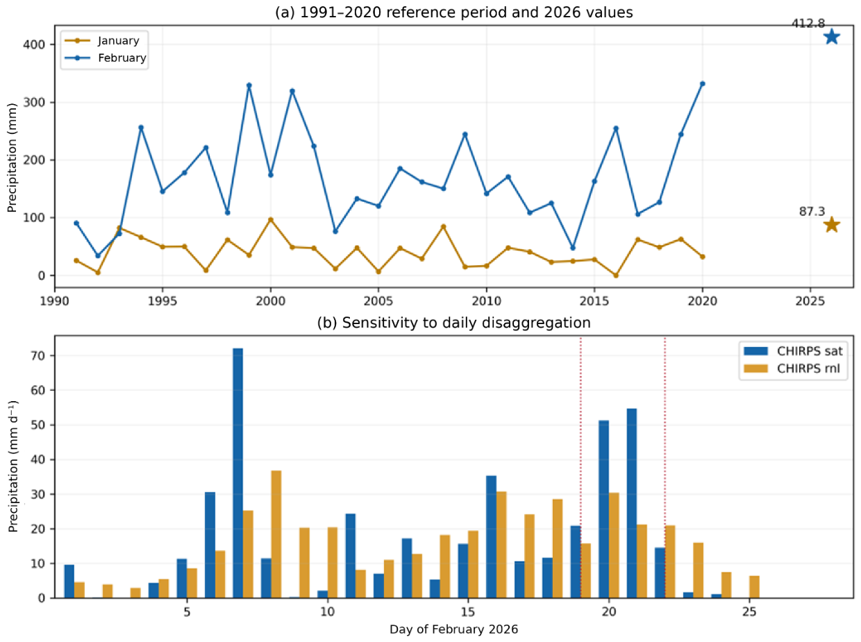
Figure 4.
Regional atmospheric conditions during the episodes of 19 and 22 February 2026, from NCEP/NCAR R1. (a, b) Specific humidity at 500 hPa (colours; g kg−1) and wind at that level (arrows; m s−1). (c, d) Convergence of vapour transport integrated between the surface and 300 hPa (colours; mm d−1) and integrated vapour transport vectors, IVT (arrows; kg m−1 s−1). Green tones indicate convergence and brown tones divergence. Each panel represents the average of 18:00 UTC on the indicated day and 00:00 UTC on the following day, equivalent to 13:00 and 19:00 PET on the same local day. The red star marks the location of the receptors and the box delimits the regional domain used in Table 4.
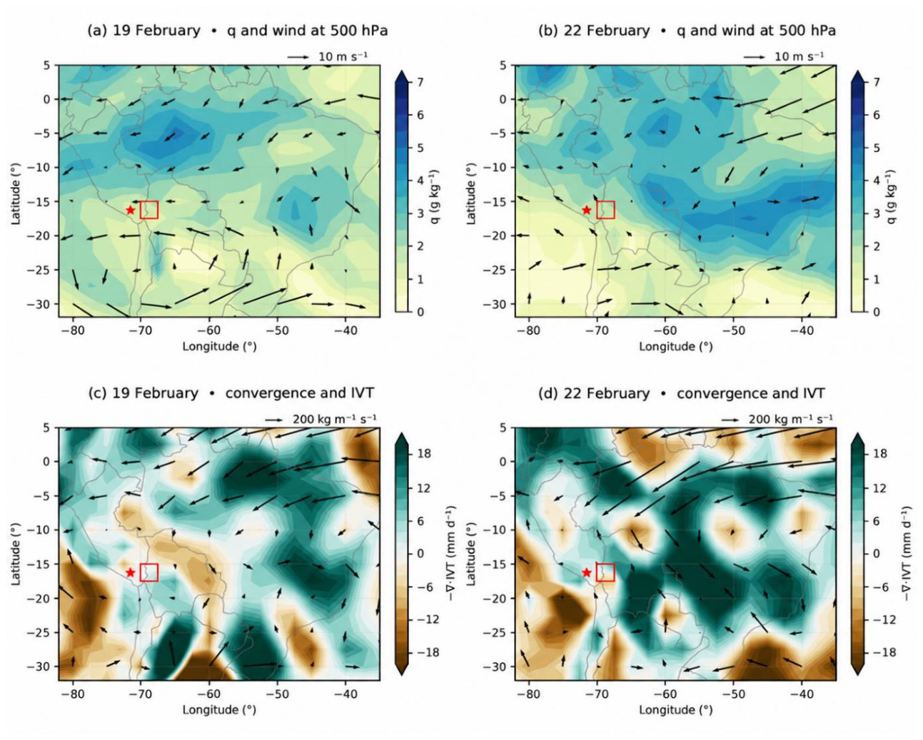
Figure 5.
Air Mass RGB composite from the geostationary ring (GOES-East/ABI over South America). (a) 19 February 2026 at 21:00 UTC (16:00 PET) and (b) 22 February 2026 at 21:00 UTC (16:00 PET). Green tones indicate tropical air masses; red and orange, dry air at mid and upper levels; blue and violet, cold air masses; and white, thick high cloud. The red star indicates the location of Arequipa. (Source: NASA Worldview).
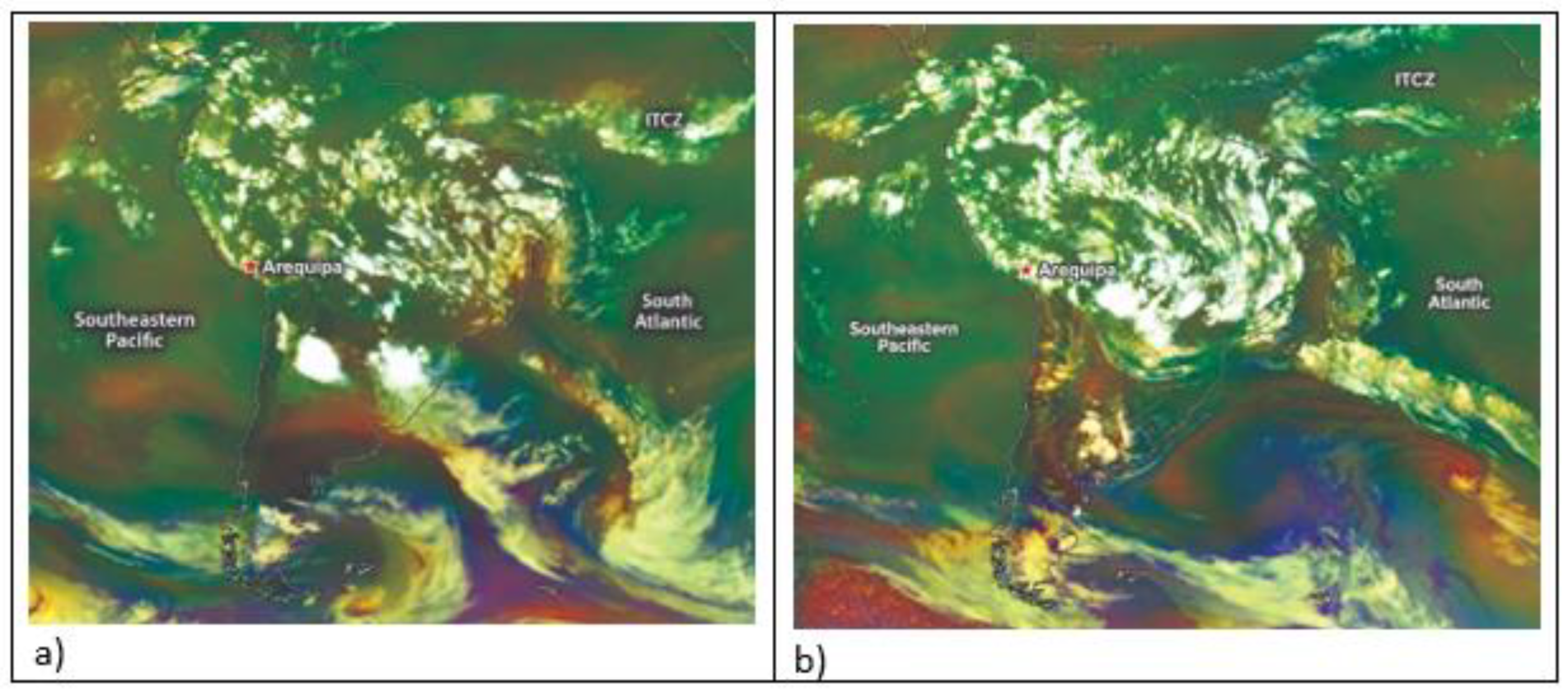
Figure 6.
Horizontal projection of the backward trajectories computed with NCEP/NCAR R1 and a 15 min integration time step, arriving on 19 February 2026 (left) and 22 February 2026 (right). Each episode includes 27 members, corresponding to three receptors, three pressure levels and three arrival times. Colour indicates days before arrival, from 0 (violet) to 10 (yellow), and the star marks the reference location of the receptors. All 27 trajectories for 19 February completed ten days. For 22 February, nine completed that interval and 18 were interrupted earlier by crossing the western boundary of the domain or reaching pressures below 300 hPa. The map represents air pathways; it does not directly show the areas of moisture incorporation.
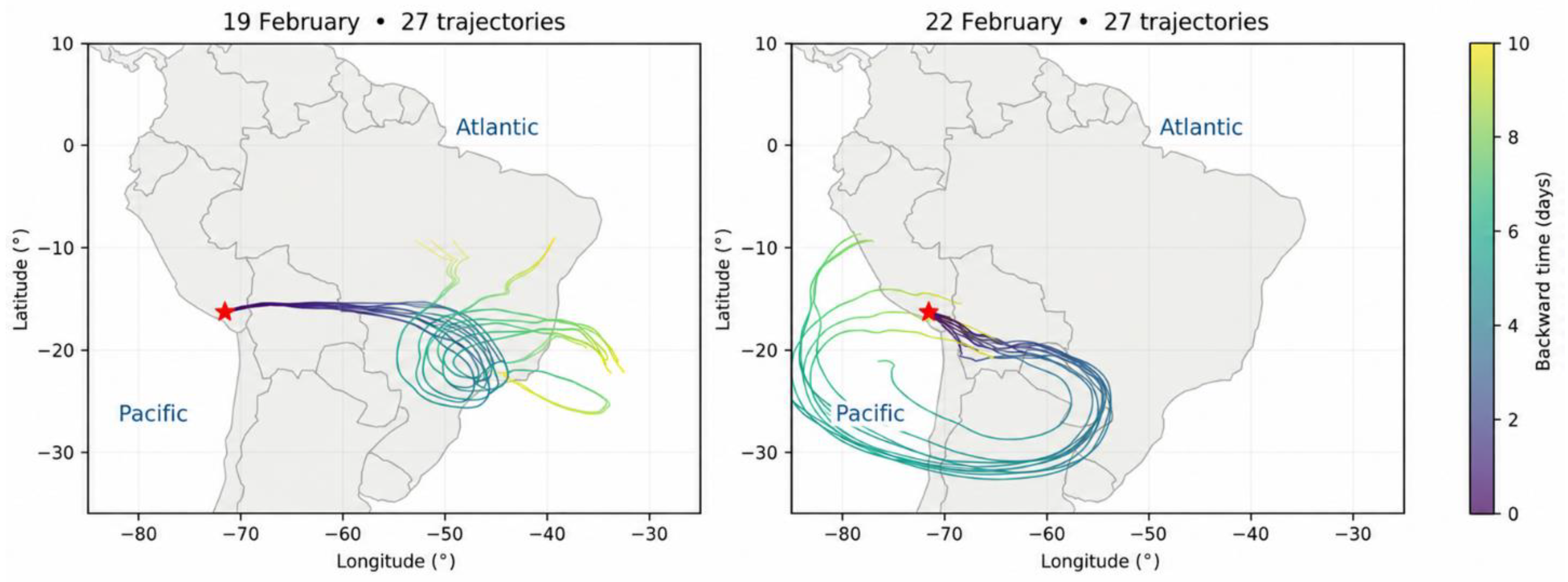
Figure 7.
Brightness temperature and extent of cold cloud tops during the episodes of 19 and 22 February 2026, from GOES-19 channel 13. Top: scenes corresponding to the minimum brightness temperature recorded within the window in the analysed samples: 19 February at 17:00 PET and 22 February at 16:00 PET. The rectangle delimits the 64-pixel window; the images are not parallax-corrected. Bottom left: hourly evolution of the minimum brightness temperature within the window. Bottom right: percentage of pixels with temperatures below −40 and −60 °C. Points correspond to hourly observations between 12:00 and 18:00 PET (UTC−5); lines only connect the samples and do not represent continuous measurements.
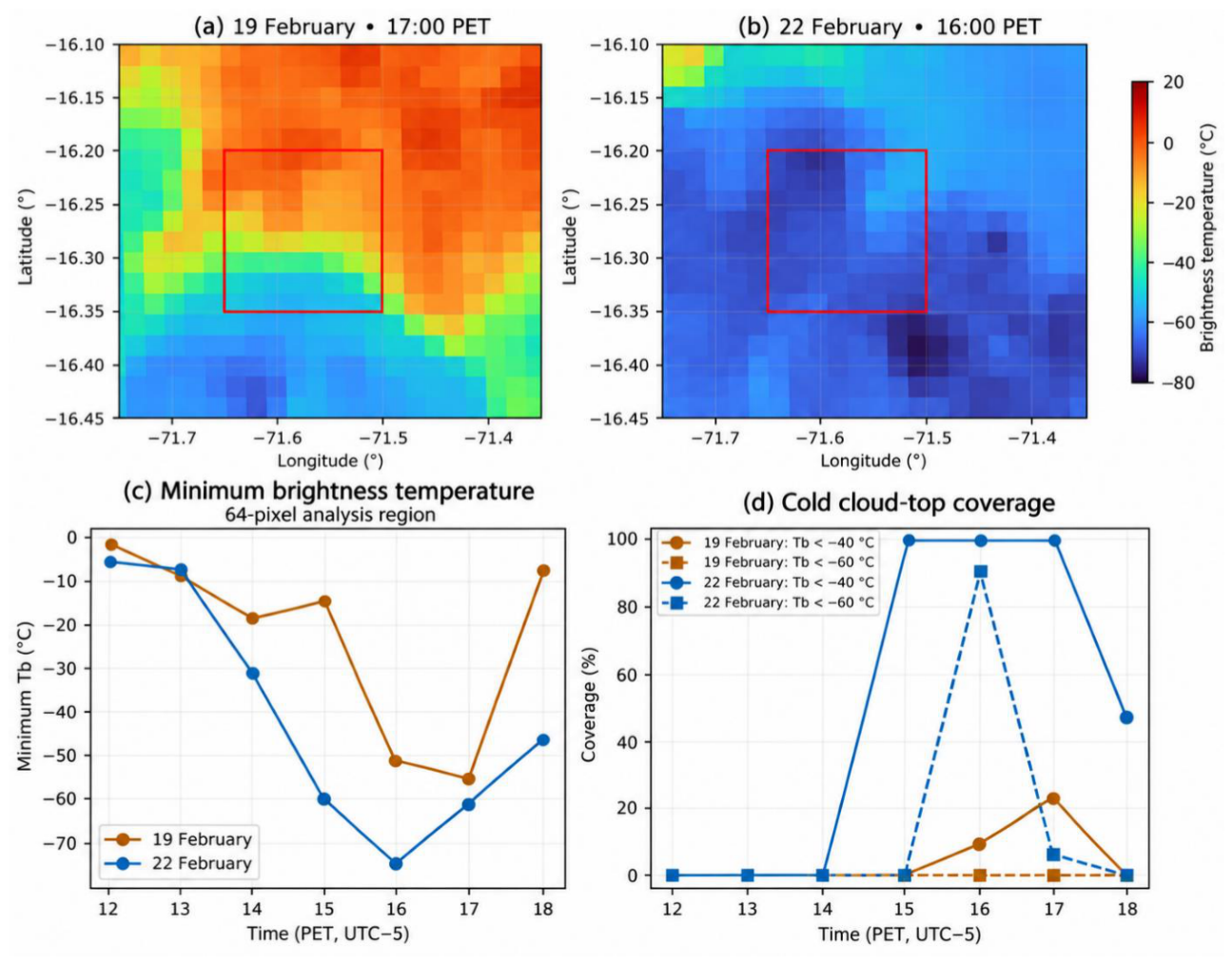

Table 1.
Products used and coverage.
| Product | Resolution | Coverage used |
|---|---|---|
| Monthly CHIRPS v3 [11,12] | 0.05° | January and February of 1991–2020 and 2026 (62 fields) |
| Daily CHIRPS v3 final, sat and rnl [12] | 0.05°; daily | 1–28 February 2026 (56 fields) |
| NCEP/NCAR R1 [20] | 2.5°; 6 h; 8 pressure levels | 29 January–24 February 2026 (108 time steps) |
| GOES-19 ABI, channel 13 [21] | 2 km; hourly (first scene of each hour) | 19 and 22 February, 12:00–18:00 Peru time (PET = UTC − 5; 14 scenes) |
| Air Mass RGB, geostationary ring (GOES-East/ABI over South America) [22] | Three-hourly; global mosaic | 19 and 22 February 2026, 21:00 UTC (16:00 PET); South America and adjacent oceans |
| NOAA CPC oceanic indices [13] | Monthly regional means | January and February 2026 |
| Terrain Tiles; Natural Earth [19,24] | Zoom 10; 1:110 M | Relief; land–ocean mask |
Table 2.
CHIRPS v3 precipitation in the window and position relative to 1991–2020.
| Indicator | January | February |
|---|---|---|
| 2026 total (mm) | 87.29 | 412.79 |
| 1991–2020 mean (mm) | 40.18 | 168.22 |
| 1991–2020 maximum (mm) | 96.85 | 332.17 |
| 2026 anomaly (%) | +117.3 | +145.4 |
| Reference years exceeded | 29 of 30 | 30 of 30 |
Table 3.
Episode precipitation and antecedent accumulation according to the daily disaggregation (mm).
Table 3.
Episode precipitation and antecedent accumulation according to the daily disaggregation (mm).
| Indicator | 19 sat | 19 rnl | 22 sat | 22 rnl |
|---|---|---|---|---|
| Episode day | 20.89 | 15.74 | 14.52 | 20.89 |
| Seven preceding days | 102.47 | 144.73 | 199.97 | 170.21 |
| Three preceding days | 57.46 | 83.51 | 126.91 | 67.34 |
Note: The antecedent windows exclude the day of the episode: they correspond to 12–18 and 15–21 February for seven days, and to 16–18 and 19–21 February for three days, respectively.
Table 4.
NCEP/NCAR R1 diagnostics in the regional domain (70–67.5° W; 15–17.5° S).
| Date and time (PET) | u500 (m s−1) | q500 (g kg−1) | IVT (kg m−1 s−1) |
C (mm d−1) | ω500 (Pa s−1) |
|---|---|---|---|---|---|
| 19 Feb, 13:00 | −6.54 | 1.34 | 47.4 | −1.62 | +0.157 |
| 19 Feb, 19:00 | −6.54 | 1.26 | 36.9 | +5.30 | +0.004 |
| 22 Feb, 13:00 | −0.94 | 1.80 | 18.8 | −3.50 | +0.057 |
| 22 Feb, 19:00 | −4.94 | 1.76 | 97.6 | +3.63 | −0.054 |
Table 5.
Decomposition of arrival specific humidity.
| Episode | Horizon | Complete members | Retained initial moisture (%) | Retained increments (%) |
|---|---|---|---|---|
| 19 February | 5 days | 27 | 36.8 | 63.2 |
| 19 February | 10 days | 27 | 18.5 | 81.5 |
| 22 February | 5 days | 27 | 4.1 | 95.9 |
| 22 February | 10 days | 9 | 1.4 | 98.6 |
Disclaimer/Publisher’s Note: The statements, opinions and data contained in all publications are solely those of the individual author(s) and contributor(s) and not of MDPI and/or the editor(s). MDPI and/or the editor(s) disclaim responsibility for any injury to people or property resulting from any ideas, methods, instructions or products referred to in the content. |
© 2026 by the authors. Licensee MDPI, Basel, Switzerland. This article is an open access article distributed under the terms and conditions of the Creative Commons Attribution (CC BY) license.
Copyright: This open access article is published under a Creative Commons CC BY 4.0 license, which permit the free download, distribution, and reuse, provided that the author and preprint are cited in any reuse.