

Submitted:
08 October 2026
Posted:
09 October 2026
You are already at the latest version
Abstract
Automated dam-safety monitoring compares each pendulum reading with a prediction band from data-driven predictive models, but its operational deployment is undermined by alarm fatigue: because prediction residuals are autocorrelated, band transgressions might arrive in clustered streaks and a per-record threshold overwhelms the operator with redundant warnings. This work treats the transgressions as a binary time series whose normal behaviour is learned during training and compares three detectors, each addressing a limitation of the previous one: a Gaussian-threshold baseline (M0), a sliding-window detector with a 99th-percentile threshold whose window is sized from the residual autocorrelation (P99), and a two-state hidden Markov model (HMM) that learns the persistence of the streaks. Applied to 28 pendulums of three dams, M0 can even increase the number of flagged records, whereas the HMM flags the fewest: in the largest case study it reduces them by 58.960 % with respect to the raw transgression series and by 45.594 % with respect to P99. An identifiability criterion based on the emission separation indicates when the HMM can be trusted (20 of 28 sensors) and when to fall back to P99, and a sensitivity analysis shows that the estimates are robust in a neighbourhood of the reference initialisation, with the self-transition probability of the Normal state as the critical parameter.
Keywords:
dam safety monitoring
; pendulums
; alarm fatigue
; anomaly detection
; hidden Markov model
; prediction band
; autocorrelation
; machine learning
1. Introduction
Dam safety is a global imperative because of the catastrophic socio-economic and environmental consequences of a possible failure [1]. These critical infrastructures, designed for water management and power generation, undergo continuous structural degradation under variable environmental loads [2]. Within this setting, pendulum monitoring is a fundamental technique for tracking horizontal displacements, providing high-precision data on the structural response to hydrostatic thrust and thermal variation [3,4,5]. Dam behaviour has traditionally been interpreted with the Hydrostatic–Season–Time (HST) model [1,6]. The present work does not propose a new predictive model: it builds on a previously developed greedy weighted stacking of BRT, RF, NN and HST models [7,8], here with SVM in place of RF, which provides the normality band whose transgressions —observations falling outside the band, also referred to in the literature as exceedances or band exceedances, and termed transgressions in this work— are the object of study here.
Despite the predictive success of such models, their operational deployment faces saturation by false alarms, or alarm fatigue — a term widely used in healthcare [9], and also popularised in cybersecurity [10] and industry, where the expression “alarm rationalization” is sometimes used [11]. Traditional thresholds tend to be inadequate for highly autocorrelated series: because serial dependence in the residuals causes transgressions to occur in clustered bursts, these repeated transgressions frequently overwhelm the operator [12,13]. Consequently, a transgression of the normality band is, on its own, a poor trigger for a warning.
The dam literature already acknowledges this excess of warnings and proposes several ways of containing it: adapting the width of the prediction band to how well the current load combination is represented in the historical data [14], confirming a warning across several sensors [15], or issuing it only after the transgression has persisted for a number of consecutive readings [14,16]. In the latter case, the required persistence is a parameter fixed a priori and applied uniformly, regardless of how strongly each sensor’s transgressions cluster under normal operation. Tuning it from data is not straightforward either: from a machine-learning perspective, the problem involves data-related challenges such as the absence of labelled anomalies —records of real damage are scarce or non-existent [17,18]— and autocorrelated errors [12]. This work replaces the hand-set persistence with one learned, sensor by sensor, from the transgressions observed during the training period, so that a warning is raised only when the behaviour of the transgressions in operation departs from the learned behaviour.
Despite these advances, a methodology that learns the stochastic patterns of the transgressions themselves during training — so as to filter redundant alerts and prevent operator desensitisation [19] — is still lacking. In particular, Hidden Markov Models (HMMs) have scarcely been applied to dam safety, even though they are a consolidated tool for modelling states and their duration in time series across many other domains [20,21,22]. Closer to the present approach, other work seeks to make anomaly detection and warnings more intelligent within dam and structural engineering itself: Nguyen [23] formulated a real-time Bayesian framework where an anomaly is explicitly pre-defined as an unexpected kinematic acceleration in the structural baseline (after isolating reversible environmental effects); a Switching Kalman Filter then adapts to this formulation by toggling between a Normal state (where baseline acceleration is strictly constrained to zero) and an Abnormal state (where acceleration variance is active), issuing an alarm whenever the posterior state probability peaks without requiring labelled failure data during training. Complementarily, Silva-Cancino et al. propose KDE-based adaptive thresholds that adjust to the evolution of ageing dams according to data representativeness [14], and Tshireletso and Moyo integrate Prophet forecasting with a GMM-HMM to detect state changes before critical transgressions occur [24].
A complementary strategy for handling the temporal structure of these series is sliding-window segmentation, well established in structural health monitoring for identifying local patterns and state changes without analysing the whole series [25,26]. Because the window size has traditionally been fixed arbitrarily, the autocorrelation function (ACF) has emerged as an objective criterion for setting it, after proving robust in comparative analyses of unsupervised time series [12,27]: Li et al. combined it with the partial autocorrelation to select the optimal length for outlier detection in gravity dams [28], and Yang et al. likewise relied on the series’ autocorrelation to set the window size, avoiding an arbitrary choice [29].
The central aim of this work is to develop and apply anomaly-detection methods for pendulum series that mitigates alarm fatigue by learning the patterns of the transgressions. The key innovation is to treat transgressions not as isolated events but as a time series whose “normal” behaviour must be learned. Three detectors operating on the binary transgression series are compared: (i) a basic fixed-window baseline; (ii) an ACF-optimised sliding-window percentile detector that accounts for autocorrelation; and (iii) an HMM that models the duration of anomalous states. We hypothesise that, by statistically characterising the transgressions observed during training, the operator can be notified only when the persistence of a deviation departs from the learned patterns, thereby restoring operational trust in intelligent monitoring systems.
2. Materials and Methods
2.1. General Approach
This paper is organised in two parts. In the first, Anomaly detection methods, the tools needed to reach the objective are built in the order in which they arose: the limitations that appeared in each method are analysed, and those limitations connect with the introduction of the next method, posed as their solution. In the second, Validation of the HMM, the reliability of the model is examined: whether it can be estimated soundly and how stable that estimate is.
The figure (Figure 1) summarises this structure to aid reading: the detection chain is shown first, followed by the validation of the HMM.
The aim of these methods is to detect automatically when a sensor’s behaviour ceases to resemble that learned during the training period of Machine Learning (ML) models, flagging possible structural anomalies without overwhelming the operator with false alarms. To this end, Phase 1 converts each sensor’s raw reading into the transgression series Z by measuring the ML models error and building bands, and three detectors, aimed at identifying streaks of consecutive transgressions (Section 2.3.2), are then applied in sequence on that series. Each detector arises from a limitation of the previous one: M0 (a Gaussian threshold) might saturate when a streak appears, because it ignores the autocorrelation of the transgressions; P99 (a sliding window with the 99th percentile) resolves that saturation by measuring the actual density of transgressions, but depends on the choice of window and percentile; and the two-state HMM (Hidden Markov Model) instead learns the persistence patterns of the streaks.
The second part validates the HMM: it introduces no new detectors, but the means to decide how far the model can be trusted. It comprises two analyses, developed in the Results section. The first, the identifiability analysis, checks sensor by sensor whether the HMM can be estimated reliably, that is, whether there is enough signal to distinguish the Normal state from the Anomalous one; it yields a threshold that decides when to trust the HMM and when to rely on P99 alone. The second, the sensitivity to the Baum-Welch initial probabilities, measures how far the HMM result depends on the starting point given to the training algorithm, i.e. how stable the estimate is (questions Q1–Q3, answered by the Distant, Similar and Reference-vs-Baum-Welch scenarios).
2.2. Dam Cases
This section describes the dam cases used in this research, together with the target variables analysed. Data are available for three dams located in Spain and monitored within two different research projects: one arch-gravity dam and two gravity dams, with heights ranging from 45 to 90.55 m above the foundation (Table 1). For confidentiality reasons, no details are given on the names or the exact locations of the dams.
The readings are irregularly spaced in time. All analyses are performed reading by reading, since each new reading is the moment at which the dam’s behaviour is assessed; the analysis of the time elapsed between readings is left for future research.
Dams are equipped with a wide range of monitoring devices to control their structural safety. Among them, pendulums were selected as the target variable because their horizontal-displacement readings provide a reliable and representative indicator of the dam’s structural response. The number of pendulums included per dam reflects data availability and quality: for Dam1, data from only one pendulum were available at the moment; for Dam2, most pendulums provided good-quality series, so a large set of 23 was included; and for Dam3, only four had time series of sufficient quality to carry out the analysis. In total, 28 pendulums were analysed.
Two types of pendulum are used. A direct pendulum, suspended from an upper anchor point, measures the horizontal displacement of the dam body relative to a lower reference, whereas an inverted pendulum, anchored in the foundation and kept taut by a float, measures the displacement relative to the foundation; some blocks combine both (direct + inverted). Each device records either radial movement (in the upstream–downstream direction) or tangential movement (along the dam axis), at different elevations —crown, perimeter gallery and horizontal galleries at approximately 40 %, 60 % and 80 % of the dam height— and in blocks distributed across the abutment–valley junctions. All readings are expressed in millimetres.
The target series differ appreciably in quality across the dams, which conditions how predictable they are. The Dam1 pendulum yields a very clean signal, closely governed by the external conditions (mostly temperature) and therefore easy to predict. Several Dam2 sensors, by contrast, show noisier series whose behaviour is less straightforward to model and whose prediction is not as evident —a situation that is common in operational dam monitoring— which makes them a demanding test bed for the detection methodology.
In Dam2 and Dam3, the external conditions during the validation period depart from those observed in training. Relating the external conditions to the warnings issued is beyond the scope of this work and is left for future research.
2.3. Phase 1 — From the Raw Reading to the Transgression Series Z
The starting point of the whole methodology is to predict the behaviour of each sensor from its external conditions and its past information, so that at every instant the observed value can be compared with the expected one. This phase is not developed from scratch: it builds on the authors’ own previous work [7,8] and on the literature on modelling and interpreting dam behaviour [1,30], taken as the basis on which the rest of the system is built.
2.3.1. Per-Sensor Predictive Model
The first step is to obtain, for each sensor of the dam, a predictive model that estimates the expected displacement as a function of the external conditions —reservoir level, temperature and precipitation— and of its past values. These variables are summarised through moving averages that capture the delayed and cumulative effect of the environment on the structure, and a variable selection is performed according to predictive ability. With the selected variables, several candidate machine-learning models are fitted and later combined, following the stacking approach developed in the authors’ previous work [7,8]: Boosted Regression Trees (BRT), neural networks (NN), a Support Vector Machine (SVM) and the classical statistical HST (Hydrostatic–Season–Time) model.
Since each model exhibits different error patterns and none is optimal under all conditions, they are combined by stacking with the Greedy Weighted Algorithm (GWA), which in the authors’ previous work improves on the best individual expert by combining the experts’ prediction vectors [7,8]. The GWA assigns each model a weight βi iteratively, selecting at each step the combination that minimises the RMSE [8].
The final model —which is the GWA combination if it improves on the best individual expert— is selected by block cross-validation, where each block corresponds to one year, using as criterion the mean RMSE over the cross-validation and test folds [8]. The selected model is trained on the whole training period; its predictions over the validation period serve as the reference for all subsequent detection.
2.3.2. Construction of the Binary Transgression Series
Once the predictive model is available, the prediction error is computed for each record at instant t [8,14]:
and an approximate two-sided prediction interval centred on the point forecast is defined as [8,14,30]:
where is the standard deviation of the errors estimated over the training period, c a coefficient controlling the band width, and yt the actual value of the series at instant t. From this band the binary transgression series (Z) is built [17]:
A record with Zt = 1 (Eq. (3)) indicates that the sensor observation falls outside the prediction band at that instant, which is henceforth called a transgression [12,14,30]. The series Zt is the common input to all the detectors described below.
A set of consecutive transgressions is henceforth called a streak. In addition, when one or two in-band records (Zt = 0) separate two nearby streaks, those records should be regarded as part of the same anomalous period: they may merely split what is essentially a single streak and carry no meaning of their own. Capturing this behaviour —rather than reading Zt record by record— is precisely what the detectors introduced below are designed to do.
2.3.3. Choice of the Coefficient c = 2
The choice of c balances two opposing risks: a value that is too low increases the false-warning rate, whereas an excessive one reduces sensitivity and may let real anomalies pass [14,31]. Under the assumption that the model errors are approximately normally distributed, the probability that a record falls outside the band is, for c = 2, approximately 5 % [14,32]: accordingly, under normal operating conditions about one in twenty records may be classified as a transgression by pure statistical chance.
This tolerance level is deliberate. A more conservative value such as c = 3 —the standard in control charts, which reduces the theoretical rate to 0.27 %— would mean that only very marked anomalies leave a trace in Zt, at the risk of moderate but sustained perturbations going unnoticed. With c = 2, by contrast, unusual behaviour is recorded even when the deviation is moderate, making transgression streaks more informative for detecting progressive changes [1,17].
It is worth stressing that the proposed methodology does not depend on this particular value: c is an adjustable parameter and the methodology still works if it is modified. It therefore adapts to whatever value the operator wishes to set, although c = 2 has been used in this research.
2.3.4. False Alarms and Their Dilution in Later Stages
The cost of choosing c = 2 is a higher false-alarm rate at the most elementary level: the series Zt contains a non-negligible number of ones that do not correspond to any structural anomaly, but to the model’s own random variability [14]. If those residuals were white noise, the transgressions would appear scattered and isolated, easy to distinguish from a real anomaly [30]. In practice, however, the residuals of predictive models on dam series show positive autocorrelation: the external conditions change gradually and the model does not capture them perfectly at every instant, so transgressions tend to cluster into streaks even under normal operation [12,28]. Reading Zt record by record then produces too many out-of-band points and, with them, alarm fatigue [9]; it is precisely this problem that motivates the move to the successive models described below.
The strategy adopted, in line with the literature [17], is not to read Zt in isolation but to analyse the temporal structure of the streaks by means of detectors calibrated over the training period, during which the dam is assumed to be free of structural problems. Should an incipient, progressive process already be present in that period, it would be partly learned as normal; however, its evolution would make the transgressions in operation increasingly persistent compared with the training behaviour, so it would still be flagged. These detectors learn what level of transgression clustering is compatible with the observed behaviour of the dam, so that individual false alarms are absorbed within the range of normal variability and only truly unusual streaks —in frequency, intensity or persistence— reach the warning threshold [24].
2.4. Phase 2 — Detectors on Z (M0, P99, HMM)
As outlined in Section 2.1, the detectors are presented in the order of their development, and each subsection concludes with the open problem that motivates the next one.
Once the binary series is constructed, the detection problem consists of determining whether the concentration of transgressions observed during validation is consistent with the baseline behaviour characterised during training. The most intuitive initial approach—which, as shown later, did not prove to be optimal—was to summarise this concentration using the windowed Transgression Rate (TSR), defined as the proportion of transgressions within a backward sliding window of size m at time step t:
In what follows, a flag is the signal raised to the operator indicating that the transgression series has persisted above the threshold —for longer, or more often— than expected under the behaviour learned during training. As each of the three methods estimates its own threshold over the training period, each method produces its own flags. The first two detectors introduced below (M0 and P99) rely directly on this formulation—Equation (4)—differing in the window size m employed and the procedure used to determine the threshold (statistic). In contrast, the third detector (HMM) moves away from window-based counting to exploit the sequential structure of Zt directly.
Before any threshold is applied, the windowed rate must be computed over some segmentation of the series. It can be evaluated over fixed blocks or over a backward sliding window, the latter being the standard and most consolidated strategy in structural health monitoring (SHM) for analysing local patterns [25,26]. Dividing time into fixed blocks of size N exposes the estimator to an edge effect: if a streak occurs around the boundary between two blocks, it is split between them and neither records its true proportion. The sliding window, by contrast, evaluates each record with its own recent context and does not depend on where the cut falls.
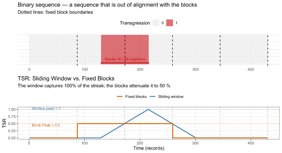
Figure 2.
Edge effect of fixed blocks on the TSR. A streak of N records misaligned with the block limits is split between two blocks (top), reducing the maximum recorded TSR to 0.5 in each; the sliding window captures it at 100 % at the instant it aligns with it.
Figure 2.
Edge effect of fixed blocks on the TSR. A streak of N records misaligned with the block limits is split between two blocks (top), reducing the maximum recorded TSR to 0.5 in each; the sliding window captures it at 100 % at the instant it aligns with it.
With an unfavourable alignment, the sliding window records TSR = 1.0 while the blocks reach only 0.5: a percentile threshold computed over blocks is lower than the true one and set too low, generating an excess of false alarms. Moreover, the number of blocks available in training is small, so the percentile estimate is less robust than with the sliding window. The sliding window is therefore adopted for all the detectors below; its size, however, has a direct effect on the result and must be chosen rigorously, as discussed for the P99 detector (Section 2.4.2).
2.4.1. M0 — Gaussian Threshold on the Windowed Proportion
The most intuitive approach, and the baseline of this research, takes a block of recent records, computes the out-of-band proportion, and compares it with the behaviour observed during training [25,26]. If that proportion is “excessively high”, the record is flagged.
M0 evaluates the TSR of Equation (4) over a fixed window of w = 30 records. To define what counts as “excessively high”, a simple probabilistic model is invoked: if the Zt were independent Bernoulli variables with parameter p = P(Zt = 1), then by the Central Limit Theorem (CLT) the windowed TSR would be approximately Normal,
which for w≈30 motivates both the window size and the use of a Gaussian threshold (6).
Importantly, the reference proportion and its dispersion are not taken from this theoretical model but estimated empirically: the mean and standard deviation of the rolling TSR are computed over the training period, and the threshold is set as
using only the upper bound, since a lower-than-expected transgression frequency is not anomalous and the TSR is bounded below by zero. Under independent, normally distributed errors the individual transgression rate would be about 5 % (for c = 2), so one might expect [14,32]; in practice, however, the residuals are autocorrelated (Section 2.3.4), and the estimated over training is typically higher than that 5 %, but might be lower than the longest streaks.
This is where the limitation of M0 becomes apparent. On the one hand, averaging over a fixed window of 30 blends isolated points with streaks: a short streak is diluted into the mean and barely raises the TSR, so the method does not separate a single transgression (noise) from a sustained streak [17] — a dilution effect discussed again for P99 (Section 2.4.2). On the other hand, the Gaussian threshold rests on the independence assumed in Equation (5), which the autocorrelated Zt violate [12,14]: the independence model understates its true variability and a symmetric threshold describes it poorly — and the higher empirical does not remedy this, since the threshold still stays low relative to the fluctuations that streaks produce. In consequence, M0 reacts to the mere clustering of transgressions rather than to genuinely unusual streaks.
The need to measure the actual density of transgressions —respecting their temporal structure instead of assuming independence— leads to the P99 detector, a non-parametric alternative based on data representativeness.
2.4.2. P99 — Sliding Window + 99th Percentile
The idea that resolves the saturation of M0 is to require a minimum density of transgressions before flagging, setting the threshold from the actual observed variability —an empirical percentile, not a Gaussian distribution— so that the autocorrelation of the streaks does not make it too permissive, as it did with M0 [14]. This adopts the principle of temporal persistence, whereby a real anomaly must manifest as a consistent deviation over time [17].
To make this concrete, P99 uses the same windowed transgression rate of Equation (4) over the backward sliding window already shown preferable to fixed blocks (Section 2.4), now with a window of size m = N whose value is decisive and is calibrated from the autocorrelation of the residuals (below). The threshold is no longer derived from a Gaussian hypothesis but obtained as the 99th percentile of the empirical distribution of over all training windows,
so that a record is flagged when over the validation period, which is equivalent to requiring an absolute number of transgressions k=⌈θ ⋅ N⌉ within the window.
Window size via the autocorrelation function (ACF). The size N has a direct effect on the value of θ, so its choice is not arbitrary: it is determined from the autocorrelation structure of the residuals, a systematic Window Size Selection approach widely supported in time-series analysis [27] and validated specifically in dam monitoring [28]. It is crucial to note that this ACF is computed on the continuous series of prediction errors et and not on the truncated binary series Zt; since the latter is inherently sparse and dominated by zeros under normal conditions, it lacks the information density required to estimate the system’s temporal memory stably, which is instead faithfully encoded in the continuous variability of the residuals [28]. The ACF of the error et measures the memory length of the series; the first lag L at which the autocorrelation falls within the noise band () marks the horizon beyond which two observations are approximately independent [28]. Since Zt = 1 when , the methodology assumes that this dependence transfers directly to the binary series, causing transgressions to cluster into streaks of typical duration L. To ensure the window is wide enough to span the whole streak and average its density properly, a window size N≈L is adopted.
The choice of the ACF rather than the PACF rests on the physical and stochastic nature of the anomaly streaks. Whereas the PACF mathematically removes the influence of the intermediate lags to isolate only the direct correlation between two instants (Xt and Xt−k), the ACF measures the total correlation, cumulatively incorporating the indirect effects transmitted through the intermediate records [28]. In dam monitoring, a real anomaly or a degradation process does not manifest as an isolated, independent jump but as a persistent, physically continued deviation over time —a streak in which each transgression is linked to the previous and the next through a chain of mutual dependencies [17]. Because the residuals show strong positive autocorrelation and tend to cluster into dense bursts [12,14], the total memory length of the process —needed to size a window that spans the whole streak— is faithfully reflected in the decay horizon of the ACF [28]. Using the PACF instead would restrict the analysis to the pure order of the underlying autoregressive process (typically AR(1) or AR(2)), drastically underestimating the true temporal extent of the transgression clusters and yielding windows too narrow to average the density of the failures [27,28].
The window is also taken backward (causal) rather than symmetric, because in operation only the past is available; a centred window would need future records not yet observed and would introduce a delay of N/2 records in issuing the flag. If the window size is well defined by the ACF, the value of θ is practically the same with either variant; only the instant of first detection changes.
Finally, when the ACF imposes a window that is too small (L = 2 or 3), the 99th percentile of the training TSRs may equal 1 —typically all records in the window are transgressions— and the detector would never trigger, since the condition is impossible. To avoid this degenerate behaviour a minimum window size is adopted: if the P99 with the N dictated by the ACF equals 1, N is increased to the next value for which the percentile is strictly below 1, ensuring the detector is operative.
Choice of the 99th percentile as the threshold statistic.
It remains to choose the statistic that turns the windowed density into a threshold. In M0 this role was played by the windowed mean of the TSR together with a Gaussian dispersion, which proved a poor descriptor of the bursty rate (Section 2.4.1); P99 instead uses a percentile of the empirical TSR distribution estimated over training, a statistic that reflects the actual density of transgressions rather than a single descriptive value. Such a single descriptive value —for instance, the maximum streak observed in training— is a weaker choice: using the maximum streak summarises the whole series in a single number, that of the longest stretch. It is unstable, since it depends on a single episode, and it does not measure density: it does not distinguish a compact streak from a scattered one with gaps. For example, a stretch made of several short streaks very close together —three transgressions, one in-band record, two transgressions, two in-band records, three transgressions and, after another in-band record, two more transgressions (11101100111011)— concentrates a clearly anomalous density of out-of-band points; yet its maximum streak (three) is no different from that of an ordinary streak, so a threshold based only on the maximum streak would not detect it. The sliding window, by averaging all those nearby transgressions within its TSR, does register the high density and correctly identifies it as anomalous.
A high percentile is chosen because it only triggers at densities that barely occurred in training: by construction, only about 1 % of the training windows exceed it. Since consecutive windows overlap, their exceedances are not independent but occur in blocks, so this 1 % describes the training windows and does not translate into an expected false-alarm rate in operation. It is demanding enough that the usual variations of the TSR —caused by autocorrelation or extreme environmental conditions— do not produce flags, but not so restrictive as to require extremely rare concentrations. The specific choice of percentile is, nonetheless, subjective and could be adjusted according to the system’s risk tolerance.
The windows overlap because this is exactly how the detector operates: at each new reading, the TSR is computed over the last N readings. Building the training distribution with the same overlapping construction makes the threshold and the statistic evaluated in validation directly comparable, since the threshold is taken from the TSR as it would have been observed, reading by reading, during training. The dependence between overlapping windows does not bias this empirical quantile, but it reduces the effective number of independent windows, so the threshold is estimated with less precision. With the few hundred windows available, the 99th percentile approaches the highest densities observed in training and is therefore partly exposed to the instability attributed above to the maximum streak; unlike the maximum streak, however, it is computed over the densities of all windows, so it still captures scattered streaks with gaps that the maximum streak ignores. This residual sensitivity to a few training episodes is one of the reasons for moving to the HMM, whose parameters are estimated from all the transitions of the series.
Even so, the method retains a weakness: the result is sensitive to the window size —hence the ACF calibration—, but it must still be chosen rigorously. A window that is too small makes the estimated threshold so high (up to the maximum possible) that the detector never triggers, however anomalous the validation period. A window that is too large, by contrast, dilutes real short streaks and mixes regimes: at the start of validation it drags in records from the end of training and generates artificial flags. To this is added that the choice of percentile, as noted, does not derive from any principle that makes it optimal in general.
To stop depending on a window, the approach is changed: instead of counting transgressions in a stretch, the aim is to learn the patterns of the streaks during training —how transgressions chain together, how long they tend to persist— and to check whether, in validation, the series still follows those patterns or departs from them. That is, the problem becomes one of predicting sequences: modelling how records succeed one another in order to recognise when the behaviour ceases to resemble the learned one. Hence the move to the two-state HMM.
2.4.3. HMM — Two-State Hidden Markov Model
The underlying difficulty is the following: estimating a long pattern all at once in a frequentist way fails, because if one wanted the probability of a specific long streak by counting how often it appeared in the historical record, it would almost never have been observed enough times and the denominator would tend to zero [20]. Decomposing the problem into one-step transitions is, by contrast, estimable with little data: there is no need to re-encounter the same long pattern repeatedly; it suffices to look, one by one, at what happened right after each 0 and each 1 (Equation 8), for which there are far more cases to average [20,21]:
This can be estimated by a Markov model: with two possible values in the transgression series (0 and 1), only four numbers are needed to form the transition matrix of a Markov chain. However, this solution applied on the raw series Zt is not enough because there t depends only on t − 1: to predict today one looks only at whether yesterday was 0 or 1, ignoring the more distant past. In the sequences 00001000 and 11101000 the transition from t = 4 (a 0) to t = 5 (a 1) would be worth the same to such a model, yet here that 1 also depends on the preceding ones, which we assume are caused by some unobserved underlying factor —and an isolated zero should not erase that memory. The solution is to introduce that “underlying factor” as two latent states (Normal / Anomalous) that emit the 0/1 with certain probabilities: the memory then lives in the hidden state, not in the last observation, and a streak survives isolated zeros [20,24,33]. Therefore, the Hidden Markov Model (HMM) method emerges.
Formally, the binary series Zt ∈ {0,1} is modelled as the observable emission of a latent Markov process St ∈ {N,A}, with N the Normal state and A the Anomalous one. The model is determined by six parameters: two emission parameters, ε = P(Zt = 1∣St = N) and ρ = P(Zt = 1∣St = A) with ε < ρ; two transition parameters, pNN and pAA; and the initial distribution πN,πA. The emission matrix B and the transition matrix A are [20,22]:
The key to the model (Equation (9)) is the separation ρ≫ε: state A generates transgressions at a much higher rate than N, so that dense streaks of Zt = 1 are evidence that the process has transited to A; the persistence pAA controls how strongly it tends to remain there [20].
The term Anomalous refers to the statistical behaviour of the transgression series, not to the structural condition of the dam. The training period is assumed to be free of structural problems, but it still contains streaks of transgressions whose origin —residual autocorrelation, limitations of the predictive model, unusual external conditions or an incipient problem— cannot be established from the data. State A captures this regime of persistent transgressions, so its presence during training is expected; what the model learns there is how long such stays typically last. During validation, a stay in A is therefore not a warning in itself: a flag is raised only when its duration is atypically long with respect to that learned behaviour (Equation (11)).
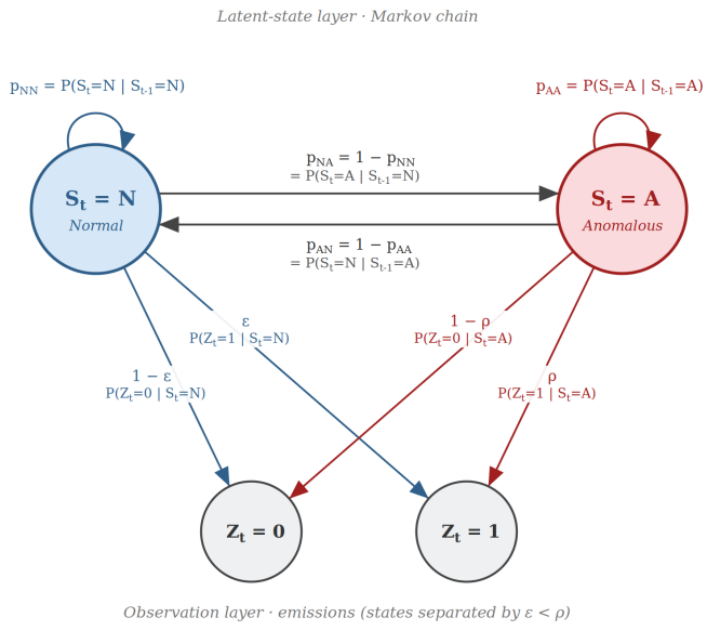
Figure 3.
Structure of the two-state HMM. Each latent state (St = N, Normal; St = A, Anomalous) emits the observations Zt = 0 and Zt = 1 with the probabilities of matrix B (ε, 1 − ε, ρ, 1 − ρ) and evolves according to the transition matrix A; the self-transitions pNN and pAA control the persistence of each regime. Image generated with Claude (Opus 4.8) following the authors’ instructions.
Figure 3.
Structure of the two-state HMM. Each latent state (St = N, Normal; St = A, Anomalous) emits the observations Zt = 0 and Zt = 1 with the probabilities of matrix B (ε, 1 − ε, ρ, 1 − ρ) and evolves according to the transition matrix A; the self-transitions pNN and pAA control the persistence of each regime. Image generated with Claude (Opus 4.8) following the authors’ instructions.
Once the model is defined, its six parameters are estimated exclusively over the training period with the Baum-Welch algorithm, an iterative Expectation–Maximisation procedure that estimates the model parameters so as to maximise the probability of the observed sequence [20,21]. Over the validation period, the most probable sequence of latent states is obtained with the Viterbi algorithm —which solves, by dynamic programming, the sequence that best explains the whole series—, while the inference of the current state relies on the posterior probabilities [20,21]. In operation, the decoding is updated each time a new reading arrives, so the state assigned to the most recent records may be revised as further readings are observed: a new transgression at time t may not be assigned to state A until the readings at t + 1, t + 2, … show whether the streak continues. This introduces a small delay in the flag, but it does not alter the flagging rule.
That fit, however, is a local optimisation over a non-convex likelihood surface, sensitive to the starting values and guaranteed to converge only to a local maximum [20]; it may therefore depend on the initial probabilities from which Baum-Welch starts. This motivates the structured initialisation described next.
With a purely random initialisation there is a high risk of converging to physically meaningless solutions or of suffering label switching, whereby models with different parameters turn out to be statistically equivalent. Structured initial estimates are therefore set that reflect heuristic knowledge of the physical system; experience with these algorithms indicates that having good initial estimates of the emissions B greatly helps to achieve a fast and correct convergence [20]. Specifically, to force the model to associate state N with calm periods and state A with persistent streaks, asymmetric initial estimates are designed [20]. It must be stressed that these initial probabilities are not the final probabilities estimated by Baum-Welch, but only a starting point, and they will be justified later on in following sections.
Initial emission matrix.
Under the hypothesis that transgressions are rare in normal operation but frequent in the anomalous state, the initial transgression probability in state N is set to the mean Z = 1 rate observed in training (similar to, or somewhat above, the theoretical 5 % of c = 2 once mixed with streaks [14]), with a floor of 0.02 to avoid numerical degeneration. For state A, the initial transgression probability (ρ) is set to the value of the threshold θ of Equation (7) —the 99th percentile of the TSR computed by the P99 method—, which defines the unusual transgression rate above which behaviour is considered anomalous. It is essential that ρ remains well above ε: if they come too close, the model can no longer distinguish Normal from Anomalous, a situation that arises when there are few streaks.
Initial transition matrix.
It must reflect the strong temporal persistence of the normal state and a high or moderate persistence in the anomalous one, under the physical premise that the dam operates in a healthy regime most of the time and that any structural degradation process is continuous and slow in time [24]:
The self-transition models that leaving the healthy state is an infrequent event, and sets an initial inertia in the anomalous state, consistent with an anomaly not dissipating immediately but tending to generate a persistent streak [24].
Initial probability vector.
Since the analysis begins by assuming the structure is healthy at the start of the series, the Normal state is strongly prioritised. As an initial proxy, the empirical frequency of the transgressions observed (the series Zt) during the training period is used, so that π = [πN,πA] = [1 − ε,ε]≈[0.95,0.05]. As the states are latent and not directly observable, this initialisation heuristically assumes that the probability of starting in the calm state (N) resembles the non-transgression rate (1 − ε) obtained under normal operation, while the probability of starting in the anomalous state (A) is associated with the mean transgression rate (ε).
The verification that these estimates do not depend critically on the starting values is carried out through a systematic sensitivity analysis —a valuable methodological step in HMMs to ensure that the iterative Baum-Welch algorithm converges robustly and is not trapped in suboptimal local minima because of the initialisation [20]—, whose methodology forms part of the validation of the HMM (below) and whose results are reported in the Results section.
The success of this fit is not guaranteed. In statistical learning, latent-variable models intrinsically present identifiability problems owing to the symmetry of their parameters [33]. In this work, to ensure the physical consistency of the system, the HMM is considered operationally identifiable if Baum-Welch estimates parameters that clearly separate the two regimes. Operational non-identifiability occurs when the algorithm undergoes a state degeneration and converges to a suboptimal local maximum with ρ≈ε [20]. In that degenerate solution both states become statistically equivalent and the model completely loses its ability to distinguish the Normal regime from the Anomalous one [20]. The underlying cause of this lack of useful convergence is the absence of sufficient transgression structure in the binary series Zt during training: if the deviation streaks are too short, too isolated, or both, the model lacks statistical evidence about the permanence in state A, preventing a robust estimation of the self-transition probability pAA [20]. The detailed analysis of when and why a particular sensor is not operationally identifiable is presented in the validation of the HMM. Under these circumstances, the degenerate HMM is not used and detection relies exclusively on the non-parametric P99 method as a fallback.
When the model is identifiable, a direct consequence of the Markov property is that the duration D of each stay in state A follows a geometric distribution: at each instant the probability of leaving A is 1 − pAA, constant and independent of how long the stay has lasted. Therefore,
If, over the validation period, the model decodes a continuous streak in the anomalous state (A) of length 𝓁, the probability that such a streak lasts that long by mere chance is given by the right-hand side of Equation (11), , where pAA is the A → A transition probability estimated by Baum-Welch during training. If this probability is below a significance level α (that is, P(D ≥ 𝓁) < α), the streak is deemed unusually long relative to the normal conditions learned and is flagged. Two significance levels are used: Moderate when P(D ≥ 𝓁) < 0.05 (a duration that by chance would occur in fewer than 5 % of cases under the calibrated model) and High when P(D ≥ 𝓁) < 0.01 (less than 1 % probability of occurring by chance). Equivalently, a streak is flagged as Moderate once its length reaches Lmod, the smallest integer satisfying , and as High once it reaches Lmod2, the smallest integer satisfying . In general, the lower this self-transition probability, the shorter the expected duration of anomalous stays, which reduces the number of consecutive records needed for the system to identify the streak as an unusual deviation.
The main limitation of the HMM is that it models the temporal structure of Zt but not the cause of the transgressions, so a streak caused by extreme external conditions is indistinguishable from one caused by structural deterioration; this and the remaining limitations are detailed in Section 3.3 (Limitations and future work).
2.5. Complementary Analyses of the HMM
This section describes the methodology of the two analyses that assess the reliability of the fitted HMM: the identifiability analysis, which decides whether the model can be trusted sensor by sensor, and the sensitivity to the Baum-Welch initial probabilities, which examines how stable the estimate is. Both are presented here at the level of method; their results are developed in the Results and Discussion section.
2.5.1. Identifiability Analysis
As noted in Section 2.4.3, when the transgression streaks are scarce and widely dispersed in time, Baum-Welch may converge to a degenerate solution with ρ≈ε [20].
The methodological key is an exact geometric property: for binary data, the difference Δ=ρ − ε is precisely the discriminative power of a single transgression to tell the two states apart, quantifying the information gained by observing one record over a purely random assignment. If the separation Δ is large (ε low and ρ high), a transgression is highly characteristic of the Anomalous state and observing a “1” gives the decoder the certainty to decide the state robustly. If Δ is small (ε and ρ very similar), a transgression is almost equally frequent in both states, so observing an out-of-band residual (Zt = 1) barely adds diagnostic information and the Viterbi algorithm loses the ability to build a coherent state sequence.
On this basis, a formal identifiability indicator (and its non-identifiability counterpart) is constructed as a diagnostic label that determines whether the fitted HMM has enough information contrast to segment the dam’s behaviour reliably or has collapsed to statistical indistinguishability. The distinction is critical in practice: a model classified as “non-identifiable” lacks the statistical robustness to be integrated safely into the reservoir’s operating protocols, and for such a sensor detection falls back to P99. The classification is built to answer one question: what threshold is appropriate to categorise identifiability in these data? In all the analyses below, each sensor’s separation is taken from its own fitted HMM, the magnitude of interest being the fitted-model separation, Δ=ρfit − εfit, computed from the estimated emission probabilities.
Analysis 1 — Separation versus evidence.
For each available sensor, two quantities are computed over the training period: the fitted separation Δ and the mean streak duration, defined as the mean length of the consecutive stretches with Zt = 1. Their association is quantified with Spearman’s rank-correlation coefficient and visualised with a 2D plot of separation versus mean streak duration. A positive correlation supports the hypothesis that the separation reached by the estimator reflects the amount of evidence (streaks) available. Beyond quantifying the association, the 2D representation allows a complementary visual reading: if the sensors group into two clouds separated by a sparsely populated band of separation values, that band naturally signals a separation value acting as a boundary between well-contrasted and collapsed models. A threshold placed in that gap would categorise identifiability robustly, leaving no sensors in the transition zone —a first empirical indication, on real data, of the range in which the criterion should be fixed. This is expanded in the Results and Discussion section.
Analysis 2 — Decoding confidence.
With each sensor’s fitted HMM, the forward–backward algorithm [20] gives the posterior probability of the Anomalous state at each record, P(A∣Z1:T). This answers a simple operational question: when a transgression appears, how strongly does the model believe the system is really in the Anomalous state? As a confidence measure, the mean of that posterior is taken over the records that are transgressions (Zt = 1) for each sensor, quantifying to what degree a transgression shifts the model’s belief towards the Anomalous state [34]. The mean is computed only over the instants with Zt = 1 because those are the records whose interpretation matters for detection: the aim is to check whether the model treats a transgression as evidence of anomaly or as an isolated deviation compatible with Normal behaviour.
This indicator is plotted against each sensor’s separation (Δ). A sufficient separation should translate into high confidence, whereas a poor one keeps it close to the prior value, a sign that the model does not commit to the Anomalous state. A value P(A∣Z1:T) = 0.5 represents indecision: given the observed transgressions and the learned temporal structure, the model assigns equal probability to both states, so a streak with posteriors near 0.5 in an unseen period could not be interpreted reliably and its classification would be unstable. Conversely, a mean posterior clearly above 0.5 means the model reads those observations as more coherent with the Anomalous state and has a probabilistic basis to keep a consistent assignment to A in a future streak.
This mean posterior is not used as a proof of the global validity of the HMM, nor as a demonstration that the estimated states correspond to real physical conditions of the dam, but as an internal decoding-confidence indicator: a confidence near 0.5 is practical evidence to set the fit aside as a segmentation tool, whereas a high confidence indicates only that the segmentation is internally consistent with the estimated emissions and dynamics. Additionally, the percentage of continuous streaks classified consistently under the Anomalous state is examined as a heuristic indicator that the model groups events robustly within the same latent state; from a physical-monitoring standpoint, the isolated in-band observations interspersed between consecutive transgressions should also be read as part of the same anomalous regime.
The final choice of the separation threshold rests on the convergence of both analyses: the relationship between separation and available temporal evidence, and the rise in decoding confidence of the transgressions beyond a certain value of Δ.
2.5.2. Sensitivity to the Baum-Welch initial Probabilities
As noted in Section 2.4.3, the Baum-Welch results are sensitive to the initial probabilities: it is an EM algorithm that converges to a local optimum, does not guarantee the global one, and the starting point may determine which optimum it reaches. This section analyses how that choice affects the final HMM estimates, through an individual analysis on an example sensor and a systematic aggregate analysis across sensors, and justifies why the chosen initial probabilities are matched to the structure to be modelled (transgression streaks = anomalous state).
The detailed justification of each initial probability was already given in Section 2.4.3; it suffices to recall that none is arbitrary but reflects what is observed in the data: pNN and pAA capture the strong persistence of both states, ε is each sensor’s background transgression rate, ρ starts from the P99 threshold (which already marks when a density is unusual), and π starts from the empirical frequency of each state in training. Throughout this section, reference initialisation denotes the initialisation finally applied in the research —the one chosen and described above— against which the remaining scenarios are compared.
The analysis is organised around three questions. Q1 — what happens with values far from those of the reference initialisation, and how do extreme values affect the parameter estimates and the results? Q2 — with an initialisation within a range similar to the reference, are the final estimates stable, or do they also vary appreciably? Q3 — how far does the final estimate move from the reference initial value; is it a substantial and consistent displacement across sensors? To answer them, the analysis is organised into an individual motivating case and three systematic analyses.
Individual analysis.
On a motivating sensor, starting from the reference initialisation, concrete changes are tested one by one and then combined: the initial distribution π is inverted (starting in the anomalous state instead of the normal one); is lowered (from 0.97 to values such as 0.70 or 0.23, to weaken the persistence of the Normal state); is lowered (from 0.95 to ≈0.10, to remove the inertia of the Anomalous state); ε(0) is raised well above the background rate; and ρ(0) is lowered towards ε (to blur the Normal/Anomalous emission separation). In each case the effect on the final estimates, on identifiability and on the Viterbi state assignment is observed. This case anticipates what is later generalised in B1/B2/B3.
Distant scenario (B1) → Q1.
It measures robustness against distant starting points. To decide whether a scenario is really “extreme”, it is compared with the natural variation of each parameter, defined as the range (minimum–maximum) of the Baum-Welch final estimates across all identifiable sensors starting from the reference initialisations; a value below that minimum or above that maximum is labelled by the percentage by which it leaves the range. On this basis, the stress scenarios of Table 9 are defined: initialisations far from the reference, a case combining several extreme parameters at once, and the reference scenario. For each sensor and scenario combination, Baum-Welch is refitted and it is computed whether the resulting HMM is identifiable and the percentage of records with Z = 1 classified by Viterbi in the Normal state (5 % ideal, being the transgression rate under normal conditions in the predictive model’s errors; 100 % total inversion), a measure computed only when the combination is identifiable.
Similar scenario (B2) → Q2.
This analysis assesses, sensor by sensor, whether small changes in the initial parameter values lead to substantially different fitted models.
For every sensor, the model fitted using the reference initialisation is first taken as the baseline. Around this baseline, a set of alternative initialisations is generated. The transition probabilities are initialised using all combinations of
Combining each value of with each value of , the transition block contains (4 × 4 = 16) combinations. These values define only the initial transition probabilities; they are subsequently updated by the Baum–Welch algorithm.
The emission parameters, ε(0) and ρ(0), are perturbed around their sensor-specific reference values. Their perturbed values are generated within a relative interval of ±15% around the corresponding reference value and are truncated to the valid probability interval [0.001,0.999]. These values are not fixed like the transition probability values because the values of epsilon and rho depend on the sensor, whereas the reference values of the transition matrix are fixed. The initial probability of state N, , is not varied independently. Instead, it is obtained from the perturbed value of , using the same perturbation width and the probability constraint
For each initialisation, the Baum–Welch algorithm is run again using exactly the same observations, model structure and convergence criteria as in the reference fit, and only the sensors identifiable with the reference initialisation are considered.
The experiments are organised into three parameter blocks:
- Transition block: and .
- Emission block: (ε(0)) and (ρ(0)).
- Initial-state block: and .
To identify the effect of each block separately, only one block is modified at a time, while all remaining blocks are kept at their reference initialisation. For example, in the transition experiment, the 16 combinations of are evaluated while the emission and initial-state parameters remain fixed at their reference values. The same principle is applied to the emission and initial-state experiments.
This design makes it possible to attribute changes in the final estimates to a specific group of initial parameters rather than to simultaneous perturbations in all parameter groups.
The combinations used in each experiment are summarised in Table 2:
For each sensor, block and combination, the final estimates are compared with those of the reference fit through two types of measure. The absolute mean deviation and its relative version quantify how far the estimates move from the reference ones, and therefore answer Q2; for a parameter such as ε, the relative deviation of a combination is
As a complement, the inter-range and relative inter-range deviations measure the dispersion of the estimates across the combinations of the grid. The deviations of each combination are then averaged across sensors, giving one mean deviation per combination and parameter for each block.
Reference vs. Baum-Welch estimate (B3) → Q3.
It measures the magnitude and consistency of the displacement across sensors. For each sensor, Baum-Welch is fitted with the full reference initialisation and, for pNN, pAA, ε and ρ, the difference between the initial and the estimated value is computed, in absolute and absolute relative terms; those differences are aggregated (mean, median, range) across sensors. In analyses B2 and B3, sensors no longer identifiable with the reference initialisation are excluded from the aggregate —their estimate with the adapted final values is not a reliable reference for comparison— and are listed explicitly in the Results. The summary metrics (degree of inversion, count of isolated points reclassified as Normal, range and deviation) are aggregated by averaging over the identifiable sensors.
3. Results and Discussion
Given the large number of sensors, the results combine metrics aggregated across sensors with representative sensor examples. Section 3.1 compares the three detectors and the number of records they flag, Section 3.2 assesses the reliability of the HMM, and Section 3.3 gathers the limitations and future work.
3.1. Anomaly Detection Methods (M0, P99 and HMM)
This section compares the behaviour of the anomaly detection methods —M0 (baseline), P99 (sliding window) and the two-state HMM— with respect to the raw transgression series Z across the three dams, in order to assess which best reduces the number of flags without failing to signal anomalous behaviour. Figure 4 summarises, for each dam and method, the number of flagged sensors and the flagged records. It should be borne in mind that Dam1 has a single sensor and Dam3 only four, so their percentages must be read with caution and the most representative reading comes from Dam2 (23 sensors).
3.1.1. Baseline Method (M0)
M0 does not reduce the number of flagged records; on the contrary, it increases them relative to Z (426 vs 346 in Dam2; 245 vs 123 in Dam3; Figure 4). It does reduce the number of flagged sensors: from 22 to 18 in Dam2 (from 95.652 % to 78.261 %) and from 4 to 3 in Dam3, while in Dam1 the single available sensor stops producing flags.
Figure 5 illustrates this behaviour on a Dam2 sensor. Table 3 shows only the methods introduced up to this point (Z and M0); the rest are added in their corresponding sections.
M0 flags every record of the validation period, increasing —as noted— the flagged records of that sensor in that period: from 73.3 % to 100 % of the validation records (Table 3), an extreme case of the method’s behaviour. As a sliding-window method, the first records of the validation period take into account the last training records within the window to evaluate the TSR and, since there are streaks at the end of the training period, the flag is raised from the very start of the validation period.
The M0 threshold is too permissive: it groups an excessive number of records as flags, to the point of flagging the entire validation period. Although it reduces the sensors with any flag in all the dams, in Dam2 and Dam3 it increases the records that the operator would have to assess, so in these cases it may not reduce alarm fatigue.
3.1.2. Sliding Window and 99th Percentile (P99)
P99 reduces the number of flagged sensors relative to Z and matches M0 (18 sensors in Dam2, 3 in Dam3 and none in Dam1) (Figure Figure 4). Moreover, it produces fewer flagged records than Z and M0 (261 in Dam2 and 131 in Dam3).
Figure 6 shows the P99 results for sensor P04626, where in the training period there are only two periods of consecutive transgressions. In the validation period there are many more transgressions, starting in 2024. The P99 method detects the anomalous period, flagging the first record where the proportion of transgressions exceeds the threshold set by the method. It does not flag the period as soon as the first transgression appears, but waits until a relative time has passed and the streak becomes anomalous within what the windows estimate.
Table 4 shows that the number of flagged records of M0 is the same as P99 (32 records, 55.2 %). Here P99 and M0 coincide, but in the next sensor they do not:

Table 4.
Number and percentage of transgressions and of flags with the M0 and P99 methods over the validation period of sensor P04626.
Table 4.
Number and percentage of transgressions and of flags with the M0 and P99 methods over the validation period of sensor P04626.
| Num. Transgressions | Z=1 (%) | Num. M0 flagged records | M0 flagged records (%) | Num. P99 flagged records | P99 flagged records (%) |
| 36 | 62.1 | 32 | 55.2 | 32 | 55.2 |
Table 5.
Number and percentage of transgressions and of flags with the M0 and P99 methods over the validation period of sensor P90710.
Table 5.
Number and percentage of transgressions and of flags with the M0 and P99 methods over the validation period of sensor P90710.
| Num. Transgressions | Z=1 (%) | Num. M0 flagged records | M0 flagged records (%) | Num. P99 flagged records | P99 flagged records (%) |
| 23 | 41.8 | 32 | 58.2 | 11 | 20 |
Here P99 reduces the percentage of flagged records to 20 %, against 58.2 % for M0 and 41.8 % of transgressions and, both in total and on average, reduces the number of records flagged for attention at all dams.
P99 raises a flag only when enough records leave the band within the window to exceed the threshold —the 99th percentile of the proportion of transgressions in the selected window—, which filters out the isolated points and streaks that do trigger the flag in Z. It improves on Z and M0 because it does not react to the first out-of-band record —which rarely indicates a real problem— but to an accumulation of transgressions close in time within the window, waiting until the evidence is sufficient. M0 may flag later, but, as shown (Figure Figure 5), it can do so by encompassing excessively long periods.
3.1.3. Hidden Markov Model (HMM)
The HMM is the method that flags the fewest records as anomalous: 142 in Dam2, against 261 and 426 for P99 and M0 respectively. This reduction is maintained on average, going from 18.522 mean flagged records per sensor with M0 to 11.348 with P99 and to 6.174 with the HMM in Dam2. An analogous behaviour is observed in Dam3, although this dam has only four sensors, of which two produce flags with the HMM and three with P99 and M0. The HMM also reduces the number of flagged sensors in Dam2, which drops from the 18 sensors with some flag under M0 and P99 to only 10 with the HMM (43.478 % of the total sensors of that dam).
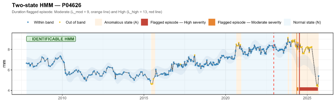
Figure 7.
Complete time series (training + validation) of pendulum P04626 (Dam2) with the states of the two-state HMM. The shading marks the anomalous state A: blue in training (period assumed free of structural problems) and red in validation (HMM flag); the red points are individual transgressions of the prediction band.
Figure 7.
Complete time series (training + validation) of pendulum P04626 (Dam2) with the states of the two-state HMM. The shading marks the anomalous state A: blue in training (period assumed free of structural problems) and red in validation (HMM flag); the red points are individual transgressions of the prediction band.
The figure 7 shows that the HMM detects the transgression streaks as periods in the anomalous state, which is precisely the aim of the method. During training, two periods in the anomalous state are identified, formed by the transgression streaks. In the second of them, a record inside the band is likewise assigned to the anomalous state —a behaviour that recurs in the other sensors where this situation arises—, which is correct, since an isolated in-band point separating two streaks should not interrupt the anomaly. Isolated transgressions, by contrast, are not assigned to the anomalous state but to the normal one, consistent with the criterion of treating them as noise rather than anomalous behaviour.
The HMM learns the patterns of both states during training and predicts them in validation. In the validation period, all the streaks are assigned to the anomalous state, but a flag is raised only when the duration of the state is atypically long with respect to the persistence learned in training (Section 2.4.3). Specifically, when the probability of reaching a given duration of the anomalous state is below 5 %, the method flags the record and starts a flagged period; as the streak lengthens, the severity increases, since that probability drops below 1 %. The flag ends when the series returns to the normal state.
In this case (Table 6) P99 and M0 produce the same percentage of flagged records, while the HMM reduces it to 44.8 %; the three methods reduce the flagged records relative to the transgression series. Moreover, the HMM raises the flags later than the other methods: it waits until the duration of the streak is atypically long compared with the anomalous stays learned in training. This waiting time is not a hand-set parameter but is estimated from the sensor’s own data, and it is what prevents clustered transgressions compatible with normal operation from being notified.
Another sensor worth highlighting is the pendulum of Dam1 (Figure Figure 8), where none of the methods raises any flag, except the pure transgression series (Table 7).
Without the anomaly-detection methods on the transgression series, all the yellow points that leave the band would be flags the operator would have to review. However, the HMM detects the streaks during the training period, classifying them as the anomalous state and distinguishing it from the normal regime of the series. In the validation period there are also streaks classified as the anomalous state, according to what was learned in training, but no flag is raised because the model has already seen streaks of that duration in the data used to estimate its parameters. Therefore, the duration of the streaks observed in validation is not anomalous, but corresponds to the usual behaviour of the series.
The HMM improves on Z and M0 because it notably reduces the flagged records by identifying, during training, the patterns of the streaks. It is the method with the strongest statistical basis and the one that best mitigates alarm fatigue, with the most coherent results.
3.2. Complementary Analyses of the HMM
This section reports the results of the two analyses described in Section 2.5.
3.2.1. Identifiability
The two-state HMM is only informative when its states —Normal and Anomalous— are statistically distinguishable. This section studies that identifiability from each sensor’s emission separation Δ=ρ − ε: it gathers the empirical evidence relating the separation to the evidence available in the data, examines the confidence with which the model decodes the states, and fixes the threshold above which a model is considered identifiable.
Analysis 1 — the separation grows with the evidence.
The emission separation reached by each sensor’s fit is related to three descriptors of its transgression streaks in training: the mean streak duration, the proportion of short streaks (≤2 records) followed by a long gap (≥3 records) and the maximum streak duration (Figure Figure 9). The separation grows with the mean (a) and maximum (c) streak duration and decreases with the proportion of short streaks followed by long gaps (b); the Spearman rank correlations confirm that the separation reached by the fit reflects the quality of the available evidence. The purpose of this analysis is not to model or predict the separation from a single descriptor, but to provide evidence that the more anomalous-state evidence there is in the data, the greater the separation tends to be. It is therefore not surprising that some sensors with null separation show values of mean streak duration —or of the other variables— similar to those of sensors with positive separation: the resulting separation does not depend on a single factor but on the combination of several (the number of streaks in training, their maximum duration, the proportion of short streaks followed by long gaps, among others), so coinciding in one variable does not imply coinciding in the separation.
Analysis 2 — the decoding confidence grows with the separation.
The decoding confidence of each sensor —the mean posterior probability of the Anomalous state over the records with a transgression (Zt = 1)— is plotted against its emission separation (Figure Figure 10). The confidence is low for sensors with small or near-zero separation and high for those with large separation, with a transition between the two regimes: below a certain separation —for the data treated here, approximately between 0.2 and 0.25— the posterior probability of Anomalous given a transgression barely departs from 0.5, whereas above it the probability approaches one. This transition confirms on real data what was anticipated in the theoretical formulation: with insufficient separation a transgression barely modifies the model’s belief, which never commits to the Anomalous state (the posterior stays close to the prior value); with ample separation each transgression is diagnostic and the model decides with certainty. The decoding confidence is thus a direct operational indicator of whether the HMM is distinguishing the states or has collapsed towards indistinguishability.
Both figures reveal a group of sensors with a practically null separation and a decoding confidence at or below chance (mean posterior ≤ 0.5): these are the models that have collapsed towards indistinguishability. As they lack a reliable Anomalous state, the sensors with a separation below 0.22 are categorised as non-identifiable, and for those sensors anomaly detection relies exclusively on the P99 method.
3.2.2. Sensitivity to the Baum-Welch Initial Probabilities
The results follow the design of Section 2.5.2: an individual case, followed by the Distant (B1), Similar (B2) and Reference-vs-Baum-Welch (B3) analyses.
Individual analysis — sensors P91039 and P90710.
Before generalising to all sensors, the effect of the initial probabilities is illustrated on two specific sensors, P91039 (Dam1) and P90710 (Dam2), to which the same types of change later analysed systematically in B1, B2 and B3 are applied. For each sensor, the reference initialisation is compared with three changes chosen among the most relevant: a robust change that does not alter the result (low pAA with high pNN), the most sensitive parameter (low pNN) and a combination that inverts the states (high ε with low ρ). Figure 11 and Figure 12 gather the four scenarios for each sensor.
In both sensors, sharply lowering pAA does not change the result with respect to the reference initialisation: the anomalous state is still decoded in the same way and the model remains identifiable. Lowering pNN with the same intensity (from ≈0.9 to 0.1) does have an effect: it markedly changes the state decoding and makes the HMM model unidentifiable. Finally, inverting the emission probabilities (high ε, low ρ) makes the fit non-identifiable in both sensors.
A simple way to understand why some changes matter and others do not is to check whether each initialisation remains coherent with the data, in which almost all records are “0” and the “1”s are very scarce. Lowering pAA barely matters: it means that it is easy to leave the Anomalous state, so there will be few anomalous stretches, and as the emission probabilities do not change, the Anomalous state remains associated with the transgressions (high ρ); few anomalous stretches fits with there being few transgressions, so the model stays identifiable. Lowering pNN, in contrast, can change the result: keeping ε low (the Normal state almost always yields “0”), setting pNN low amounts to saying that the Normal state is left continuously —that it is almost never sustained—, which does not fit a series made of very long streaks of “0” where the process is in fact in Normal most of the time. That contradiction seems to be what degrades the fit.
Finally, inverting ε and ρ leaves the model non-identifiable: keeping pNN high (the process is almost always in Normal) but setting ε high (the Normal state would often yield Zt = 1) makes the initialisation assert simultaneously that the usual thing is to be in Normal and that, while in Normal, many transgressions are seen, when the Zt = 1 are in reality very scarce; that incoherence may prevent Baum-Welch from converging to a coherent solution.
These two sensors illustrate the phenomenon but do not establish how often it occurs or whether the pattern generalises. The same type of test is therefore repeated systematically over the remaining sensors in the analyses that follow.
Distant scenario (B1).
This analysis subjects the HMM fit to initialisations deliberately far from the reference values —hence the name “distant scenario”— and applies them systematically to all sensors, in order to find out which combinations of initial probabilities end up degrading or breaking the model. To judge when a value is really extreme, the natural variation of the final estimates across sensors is first established —the range to which Baum-Welch converges starting from the reference initialisation—, and the stress scenarios are defined relative to it (Section 2.5.2). This natural variation is summarised in the table (Table 8) and boxplot below (Figure 13).
Except for pAA and ρ, the parameters estimated by Baum-Welch show a very low dispersion across sensors: the differences between maximum and minimum are barely 0.036 in ε, 0.114 in pNN and 0.132 in πN and πA, with very narrow boxes. With the reference initialisation, Baum-Welch converges to similar values in almost all sensors: pNN and πN concentrate near 1, and ε and πA near 0. The exceptions are pAA (range 0.431–0.883, difference 0.452) and ρ (range 0.259–0.831, difference 0.573), whose wide boxes reflect estimates that vary appreciably from one sensor to another.
The scenarios of this analysis are deliberately chosen outside this natural range —that is why they are “stress” scenarios. However, as the probabilities are bounded in [0,1], the room to move away is not the same for all parameters: for pNN, pAA, ρ and πN the natural range is already close to the ceiling (for example, ρ reaches 0.831 and pAA 0.883), so their real upward margin is small, whereas ε and πA, with ranges close to 0, admit a much larger upward excursion.
The aggregate response of the HMM to each stress scenario, across the 28 sensors, is summarised in the table (Table 9) and figure (Figure 14) below through two measures: the percentage of transgressions (Z = 1) that the model classifies in the Normal state (“Z = 1 in the Normal state”, where a low value is ideal —separating the streak transgressions from the random-noise ones— and a value near 100 indicates a total inversion) and the percentage of sensors in which the scenario degenerates the HMM (non-identifiable).
Table 9.
Distant scenario: response of the HMM to the stress initialisations, aggregated across the 28 sensors.
Table 9.
Distant scenario: response of the HMM to the stress initialisations, aggregated across the 28 sensors.
| Code | Category | Scenario | Z = 1 in Normal (%) | Unidentifiable sensors (%) |
| D1 | 1. Individual | pNN −74% from minimum | 10.516 | 92.857 |
| D2 | 1. Individual | pAA −77% from minimum | 20.431 | 28.571 |
| D3 | 1. Individual | ε +91% from maximum | 20.431 | 28.571 |
| D4 | 2. Pair, same block (emission) | ε +91% + ρ +8% from maximum | 20.431 | 28.571 |
| D5 | 2. Pair, same block (emission) | ρ −81% from minimum + ε +91% from maximum | 26.931 | 82.143 |
| D6 | 3. Cross-pair | ρ +8% from maximum + pNN −89% from minimum | 9.386 | 89.286 |
| D7 | 3. Cross-pair | pAA −77% + pNN −89% from minimum | — | 100.000 |
| D8 | 1. Individual | πN −88% from minimum | 17.759 | 39.286 |
| D9- REF | Reference | Reference initialisation | 20.431 | 28.571 |
| D10 | 4. Extreme case | pAA −77% + ε +91% + ρ −81% + πN −88% | 17.759 | 39.286 |
| D11 | 1. Individual | ρ −81% from minimum | 22.751 | 46.429 |
| D12 | 2. Pair, same block (transition) | pNN −74% + pAA −77% from minimum | — | 100.000 |
Note: “Z = 1 in Normal (%)” is the percentage of transgressions that the HMM classifies in the Normal state (100 = total inversion); “Unidentifiable sensors (%)” is the percentage of sensors in which the scenario degenerates the HMM. REF is the reference initialisation.
With the reference initialisation, on average 20.431 % of the transgressions fall in the Normal state and 28.571 % of the 28 sensors are non-identifiable; these are the reference values. The scenarios that alter pNN are by far the most disruptive: changing it alone (D1) already leaves 92.857 % of the sensors non-identifiable, and combining it with pAA (D7 and D12) breaks the model completely (100 % non-identifiable, with no sensor left to average over). At the opposite extreme, altering only pAA (D2), only ε (D3) or ε and ρ in a controlled way (D4) reproduces the reference values exactly.
Between the two extremes, ρ alone (D11) does have an effect —it raises the percentage to 22.751 % and leaves 46.429 % of the sensors non-identifiable— and its combination with ε (D5) is the one that most increases the percentage (26.931 %, with 82.143 % non-identifiable sensors), the most severe scenario among those that do not touch pNN. The scenarios that do not strongly alter pNN, such as D8 (πN) and D10 (all parameters at their extreme except pNN), are much milder (17.759 %, 39.286 % non-identifiable). In the figure 14, the scenarios that touch pNN (D1, D6, D7, D12) show the lowest boxes or none at all —D7 and D12 do not appear because no sensor is identifiable—, and the bar panel shows the escalation of the non-identifiable percentage up to 100 % in D7 and D12.
The clearest result is that pNN is the critical parameter: on its own or combined with any other, it is what most degrades the model, and its combination with pAA (D7, D12) is the most destructive of all, above pNN alone. This suggests that the transition block is the most fragile point of the fit under a completely wrong initialisation, even more than combining transition with emission. The behaviour of ρ is striking, because in isolation (D11) it does have an effect —unlike pAA or ε in isolation—, which contrasts with what is observed in the Similar scenario (B2), where it barely matters; the difference would lie in the magnitude of the change, much larger here. Moreover, that ε alone (D3) and the controlled ε + ρ (D4) reproduce the results of the reference initialisation indicates that the ε stress value used is demanding but assimilable by the model if ρ is maintained close to its reference value, not so far from the natural range as to cause collapse while keeping the rest at their reference values. Finally, the similarity between D10 (everything at its extreme except pNN) and the milder scenarios points to the model tolerating the rest of the parameters at their extreme as long as pNN stays at a reasonable value. All this is coherent with the observed natural variation: the parameters with a narrow range pinned to their limits (pNN and πN near 1; ε and πA near 0) are the ones that most condition the result, which fits with Baum-Welch converging to very similar values across sensors precisely in those parameters.
Similar scenario (B2).
In contrast to the previous analysis, this one checks the stability of the fit under initialisations close to the reference (design in Section 2.5.2); sensors non-identifiable with the reference initialisation are excluded from the aggregate.
Note: Mean (relative) deviation: average distance between the final estimate of each combination and the estimate obtained with the reference initialisation. Inter-range deviation: (max − min) across the grid combinations; its relative version is (max − min)/max.
Table 10 shows only the transition block produces appreciable deviations with respect to the results obtained with the reference initialisation; in the emission and initial-state blocks, both the deviation and the internal dispersion are practically null. Within the transition block, the deviation concentrates, strikingly, on parameters that were not directly perturbed: ε (≈38.92 % relative deviation) and πA (≈29.57 %) are the ones that move furthest from the reference results, while pNN and pAA themselves barely move (2.82 % and 1.77 %), as do ρ (5.12 %) and πN (3.36 %). The internal dispersion of the grid follows a similar order, with ε, πA and ρ as the most variable parameters across combinations.
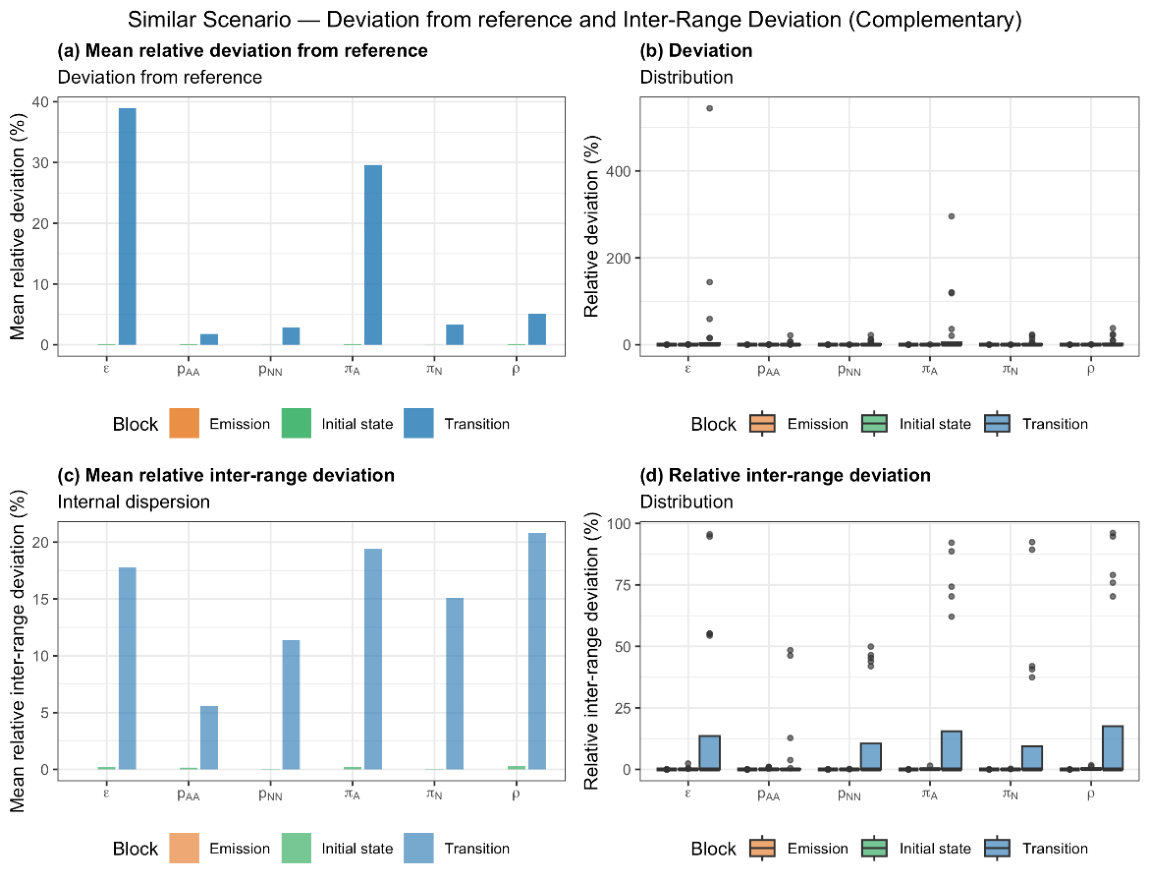
Figure 15.
Similar scenario: sensitivity of the HMM to initialisations close to the reference, by parameter and block. Relative deviation with respect to the reference initialisation, as a mean across sensors (a) and per-sensor distribution (b); inter-range deviation as a mean (c) and distribution (d). Colour groups the parameters by block.
Figure 15.
Similar scenario: sensitivity of the HMM to initialisations close to the reference, by parameter and block. Relative deviation with respect to the reference initialisation, as a mean across sensors (a) and per-sensor distribution (b); inter-range deviation as a mean (c) and distribution (d). Colour groups the parameters by block.
The figure 15 nuances this reading, however: in the per-sensor boxplot, the median and the interquartile range are practically stuck at 0 for all parameters, so in the vast majority of sensors the estimate barely moves from those obtained with the reference initial probabilities (b). The inter-range deviation (d) also shows a median around 0, although here the box of the transition block is wider, indicating more occasions in which the parameters take values between 0 % and 15 % of inter-range deviation. The high means of ε and πA come from a few atypical sensors —with deviations reaching ≈520 % and ≈300 %—, not from a generalised shift. The central tendency is therefore one of stability.
The main conclusion is that, under initialisations close to the reference, the HMM behaves stably: only the transition block moves anything, in line with what was observed in the Distant scenario (B1), where the trigger was also pNN and not the emission or the initial state. The most characteristic feature is that, within that block, the effect does not fall on the perturbed parameters —pNN and pAA stay very stable— but, indirectly, on ε and πA. A possible explanation, in line with the individual analysis, is that lowering pNN raises ε and the states tend to invert —the streaks come to be interpreted as Normal and the in-band records as anomalous—, an effect more noticeable in ε and πA because both start from small values and are therefore more sensitive in relative terms to the same change. That ρ stands out in the internal dispersion but not in the mean deviation further suggests that it varies considerably from one combination to another but without moving systematically away from the estimates obtained with the reference initialisation.
Detail of the transition block, combination by combination.
In the previous aggregate, the transition block () is the one that most moves the final estimates. Here that block is broken down combination by combination: for each combination of the grid {0.70,0.825,0.95,0.99} of , averaged over the sensors identifiable with the reference initialisation, Table S1 (Supplementary Materials) gives the final estimate of each parameter, the estimate produced by the reference initialisation (, ) and the signed relative deviation of each combination with respect to the reference values.
Before scanning the whole range of , one point (, rest = reference) is examined per sensor, not only on average, to check whether the mean is representative or hides very different sensors.
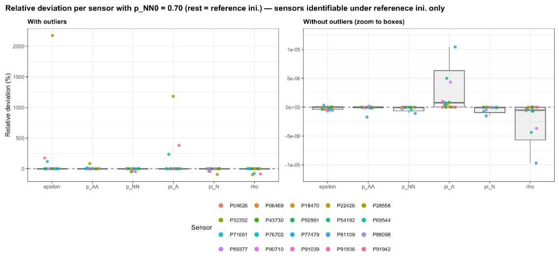
Figure 16.
Relative deviation of the final estimates with respect to the reference initialisation, by parameter and sensor, fixing
Figure 16.
Relative deviation of the final estimates with respect to the reference initialisation, by parameter and sensor, fixing
(rest at reference values); only sensors identifiable with the reference initialisation. Each point is a sensor (colour = sensor). Left panel: full scale (with outliers). Right panel: zoom to the boxes (without outliers), where the deviation is almost null for almost all sensors.
In Table S1, the rows with are the ones showing appreciable changes, and those with 0.950 and 0.990 coincide with the reference whatever is, which confirms that moving pAA is harmless and that the effect is triggered by lowering pNN. With , the largest mean deviations again occur in ε (between +123.628 % and +209.609 %) and πA (between +90.091 % and +118.352 %), while the rest of the parameters move far less. The rows with now show non-null deviations, but much smaller and not significant (at most +5.953 % in ε and +11.860 % in πA), far below those of the block. All the medians are 0, however, a sign that the change is not generalised but caused by a few atypical sensors; the figure 16 confirms this: with outliers the deviation soars (isolated points exceeding 2000 % in ε), but zooming to the boxes it is practically null for almost all sensors. The following table (Table 11) identifies those atypical sensors, the ones that fall outside the whisker of the boxplot.
The outliers that inflate the deviation are very few and repeat —P28558, P76702 and P91942—, and in all cases they cease to be identifiable with ; P76702 joins this group after the change in identifiability of the Dam2 sensor. The largest deviations concentrate in ε (P28558, 2176.483 %) and πA (P28558, 1182.371 %). This confirms that the mean deviation does not reflect a real shift of the estimates, but an artefact of degenerate fits in a few sensors with very few streaks in their training period.
To locate more precisely the value of at which the deviation begins to grow, is fixed at the reference value and is swept with many points, from 0.50 up to its adapted initial value in the reference solution (0.97), yielding a continuous series instead of four isolated points. The relative deviation (Figure Figure 17a) is computed only over the sensors identifiable with the reference initialisation, since their reference estimate is needed as the denominator; the percentage of non-identifiable sensors (Figure Figure 17b) is computed over all 28 sensors, so as not to exclude by construction those that are already non-identifiable with the reference initialisation.
from 0.5 to its reference value (0.97), with fixed at the reference. (a) Mean relative deviation of the final estimates with respect to the reference initialisation, per parameter (identifiable sensors only). (b) Percentage of non-identifiable sensors (all sensors). The red dotted line marks the reference value.
The sweep in Figure 17 shows that the deviation only appears below : from there up to the reference initial value all the curves are at approximately 0, that is, the model is insensitive to over the whole upper stretch. Below 0.80 the deviation grows in steps, led by ε (up to ≈520 % at 0.50) and followed by πA (≈230 %), while the rest of the parameters stay flat. The percentage of non-identifiable sensors follows the same pattern: it falls monotonically as rises, from ≈57 % at 0.50 to stabilising around 29 % from ≈0.80. Both transitions coincide —the zone where the estimates stabilise is the same where the non-identifiability stops increasing—, and the reference (0.97) sits comfortably within that flat zone, far from the breaking threshold (~0.80).
The detail confirms and refines what was noted in the aggregate: the HMM is stable under initialisations close to the reference, and the only parameter with an effect is , which reinforces the conclusion of the Distant scenario (B1) about its critical role, now also in the neighbourhood of the reference when there are few streaks in the training period. The high mean deviations of ε and πA do not indicate instability of the method, but the effect of a few non-identifiable sensors whose degenerate fits inflate the average; this is why the median should always be read alongside the mean. In practical terms, the sweep delimits a clear safety margin: degradation only appears below , so the reference value (0.97) is comfortably located in the stable zone, which supports the choice of the reference initial probabilities.
Reference vs. Baum-Welch estimate (B3).
The previous analyses showed how the model responds to altered initialisations; this one focuses on the initialisation actually used —the reference one— and quantifies how far the final Baum-Welch estimate moves away from it. For each parameter, the difference between the estimated and the initial value is computed, in absolute and relative terms, aggregated over the identifiable sensors (Section 2.5.2); the per-sensor detail is reported in Table S2 (Supplementary Materials).
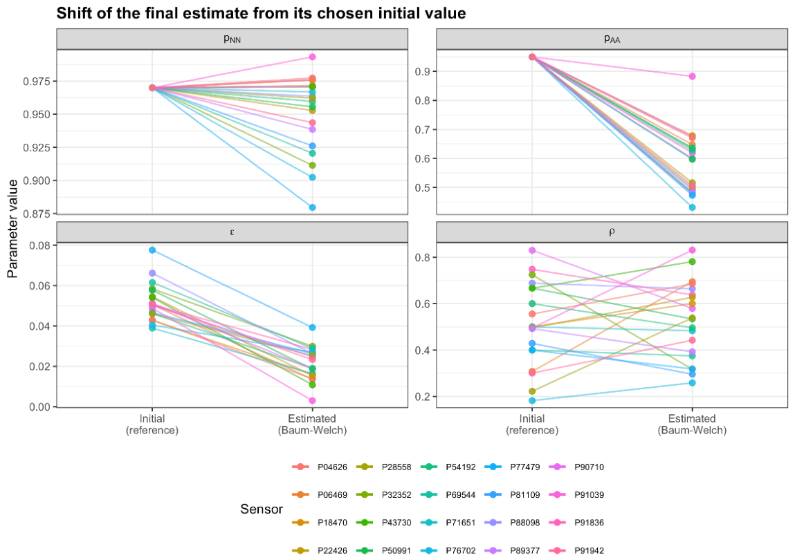
Figure 18.
Displacement of the HMM final estimate with respect to its reference initial value, per sensor. Each line joins, for one sensor, the reference initial value and the final value estimated by Baum-Welch; one panel per parameter (pNN, pAA, ε, ρ), each with its own scale. Only sensors identifiable in the reference solution; colour identifies the sensor.
Figure 18.
Displacement of the HMM final estimate with respect to its reference initial value, per sensor. Each line joins, for one sensor, the reference initial value and the final value estimated by Baum-Welch; one panel per parameter (pNN, pAA, ε, ρ), each with its own scale. Only sensors identifiable in the reference solution; colour identifies the sensor.
The displacement has its own direction and magnitude for each parameter. pNN barely moves: it stays in a narrow range (0.880–0.993; relative difference between 0.077 % and 9.314 %) and usually ends slightly below the reference value (0.97). pAA drops systematically in all the sensors (final estimate between 0.431 and 0.883; relative difference from 7.053 % to 54.607 %). ε shows the clearest direction: it decreases in 100 % of the sensors, with relative differences from 33.162 % to 93.715 %. ρ, by contrast, has mixed behaviour —it rises in 9 sensors and falls in 11— and is the parameter with the widest variation range (3.427 % to 142.486 %).
Consistent relationships appear between parameters: pAA and ε move in opposite directions across sensors, so the sensors in which pAA barely deviates are the ones that most deviate ε, and vice versa; pNN and pAA, in contrast, move in the same direction. The two most extreme ρ cases (126.021 % and 142.486 %) correspond to the two sensors with the lowest reference initial ρ (0.308 and 0.222).
That pNN barely moves is a good sign: it suggests that its reference value (0.97) already reflected reality well —the vast majority of records are normal—, so Baum-Welch hardly needs to correct it. The systematic decrease of ε is also expected: its initial value is computed over the whole training period, but by the end of the fit the model separates the truly normal stretches better, which are even cleaner than the average, so ε tends to fall. The joint behaviour of pAA and ε —both falling, in opposite directions between each other— points to the model distributing the fit between the two: when it attributes more persistence to the anomalous state (high pAA), the Normal state generates fewer “ones” and ε falls, and vice versa, so that the final result —identifying the streaks well— can be reached by different combinations. It is worth watching, though, the cases in which ε approaches zero without pAA dropping, because too small an ε would make even an isolated out-of-band point count as anomalous, exactly the opposite of what is sought. As for ρ, it is the most variable parameter, but its two extreme cases seem punctual —the sensors that started from a very low reference initial ρ, which the fit corrects strongly—, not a general problem. Overall, no sensor stays exactly the same —the reference initialisation is not a fixed point—, but the movement is coherent with what would be expected from each sensor’s data and not erratic: little in pNN, which was already well placed and is the most sensitive, and somewhat more in pAA, ε and ρ, always in a reasonable direction.
Taken together, the individual case, the Distant scenario (B1), the Similar scenario (B2) and the reference-vs-estimate comparison (B3) converge on the same ideas: pNN is by far the critical parameter —the only one that, when lowered, changes the estimates and can render the model non-identifiable—; the HMM is stable under initialisations near the reference, with degradation appearing only below , so the reference value (0.97) sits comfortably in the stable zone; and the high mean deviations of ε and πA reflect not instability but a few non-identifiable sensors with very few streaks, which is why the median should be read together with the mean. On the other hand, analysis B3 shows that the initial probabilities are not the ones ultimately estimated, but rather change to adapt to what the model observes during training. The pNN varies the least, which makes sense given that we have observed it to have the greatest impact on the model’s identifiability. All of this supports the choice of the reference initial probabilities.
3.3. Limitations and Future Work
The proposed methodology has several limitations that must be borne in mind when interpreting the results.
Cause of the transgressions. The HMM does not know why there is a transgression: it models the temporal structure of Zt but does not incorporate the environmental covariates, so a streak caused by extreme external conditions is indistinguishable from one caused by structural deterioration. In such circumstances the predictive models themselves might not yield good predictions, and the resulting streak would be flagged in the same way as a structural one.
Non-identifiability. With very few streaks, or only single-record streaks, Baum-Welch does not converge to a useful solution and P99 is used exclusively; under the adopted criterion this occurs in 8 of the 28 sensors. Moreover, the separation threshold (Δ=0.22) is not meant to be optimal in theoretical terms, but the most adequate for our case: it is the value that best separates the usable models from the degenerate ones according to the analyses of Section 3.2.1, carried out on our own data.
Uncertainty of the persistence estimates. With few streaks in training, the estimation of pAA carries large uncertainty, and the severity values derived from it are indicative, not guarantees. In dam monitoring, records of real damage are scarce or non-existent, which restricts training almost exclusively to healthy operation [18], and streaks of transgression sustained over time caused by severe seasonality or extreme external conditions are likewise scarce; because of that scarcity it is statistically impossible to verify reliably the independence-of-transitions assumption underlying the geometric distribution, which holds that the probability of leaving an anomalous state does not depend on how long it has lasted [20]. As that requirement cannot be tested, the theoretical durations of Equation (11) lose validity as exact physical probabilities and must be interpreted heuristically as a severity score or persistence index [33].
This formal limitation does not, however, compromise the method’s effectiveness in detecting anomalies. The HMM is calibrated over a period guaranteed to be healthy, in which it learns the basal persistence of the transgressions compatible with normal variability and sensor noise. Should a degradation process develop during validation, it would manifest as a dense, uninterrupted streak far exceeding the learned stochastic limits, making the Viterbi sequence remain in the anomalous state for an unusually long time and thereby ensuring the timely activation of the flag by its excessive duration.
Geometric assumption. The geometric assumption may fail under cumulative damage with its own memory (a progressive crack, a growing leak), in which case the geometric distribution underestimates the probability of long stays; this, however, makes the model conservative in the right direction, since genuinely persistent stays turn out to be even more surprising than expected and increase the sensitivity to structural anomalies.
Detection delay. By design, the detectors wait until the persistence of a streak is atypical with respect to training before issuing a warning, which implies a delay compared with a record-by-record warning; this delay is the price of reducing the alarms caused by transgressions compatible with normal operation. Quantifying it, together with the probability of detection, would require anomalies of known onset and magnitude, which are not available in the monitored dams; an evaluation with synthetic anomalies superimposed on real series is therefore left for future work.
Data. Although Dam1 contributes a single sensor (Section 3.1), it is a valuable case study: its series shows the clean, strongly seasonal pattern, governed mainly by temperature (Section 2.2), that is commonly observed in pendulum records, so it is representative of the typical behaviour that a detector will face in operational dam monitoring.
Future work. Characterising the external context of a flagged period —in order to tell whether or not it resembles the training conditions— lies beyond the detectors studied here and is a natural direction for future work, as it would address the main limitation above. In addition, the dams are equipped with a variety of monitoring devices covering different aspects of dam safety; evaluating the methodology on other sensor types is planned, aiming to provide a more holistic assessment of overall dam safety.
4. Conclusions
Automated dam-safety monitoring compares each pendulum reading with the normality band produced by data-driven models, but its operational deployment is undermined by alarm fatigue: because the prediction residuals are autocorrelated, band transgressions arrive in clustered streaks, so a per-record threshold overwhelms the operator with redundant flags. This work reframed detection at the level of the transgression streak and compared three detectors operating on the binary transgression series, introduced in the order in which the limitation of each motivated the next: a Gaussian-threshold baseline (M0), an autocorrelation-sized sliding window with a 99th-percentile threshold (P99) and a two-state hidden Markov model (HMM).
The results show a clear progression. M0 does not mitigate the problem: by ignoring the autocorrelation, its threshold is too permissive and it can flag an entire validation period, so in Dam2 and Dam3 it even increases the number of flagged records with respect to the raw transgression series (426 vs. 346 records in Dam2). P99 corrects this by requiring a minimum density of transgressions within the window, reducing the flagged records to 261 in Dam2, while the HMM, which learns the persistence of the streaks, is the method that flags the fewest records: 142 in Dam2, a reduction of 58.960 % with respect to reading the transgression series record by record and of 45.594 % with respect to P99. The same trend holds on a per-sensor basis, where the mean number of flagged records in Dam2 falls from 18.522 with M0 to 11.348 with P99 and to 6.174 with the HMM, and the number of flagged sensors drops from 22 to 10. Moreover, the HMM raises its flags later —only when the duration of an anomalous streak is atypically long with respect to what was learned in training— and correctly absorbs the isolated in-band records that separate two nearby streaks, while treating isolated transgressions as noise. It is therefore the method with the strongest statistical basis and the one that best mitigates alarm fatigue.
As the HMM is a latent-variable model, its reliability was assessed before drawing these conclusions. An operational identifiability criterion based on the emission separation Δ=ρ − ε was proposed: the separation was shown to grow with the amount of evidence available in the data (Spearman correlations of +0.95 and +0.87 with the mean and maximum streak duration, respectively) and with the model’s decoding confidence, and an empirical threshold of Δ=0.22 was fixed to decide when the HMM can be trusted and when detection must fall back to P99; under this criterion, 20 of the 28 sensors were identifiable. A systematic analysis of the sensitivity to the Baum-Welch initialisation further showed that the estimates are stable across a wide neighbourhood of the reference initial probabilities: only the self-transition probability pNN has an appreciable effect, and the model degrades only when it is initialised below ≈0.80, so the reference value of 0.97 lies comfortably within the stable region. This supports the robustness of the adopted initialisation.
The main limitation of the approach is that the HMM models the temporal structure of the transgressions but not their cause, so a streak driven by extreme external conditions cannot be distinguished from one driven by structural deterioration; this and the remaining limitations, together with the future research lines, are detailed in Section 3.3. Overall, treating band transgressions as a time series whose normal behaviour is learned during training —rather than as isolated events— makes it possible to notify the operator only when the persistence of a deviation departs from the learned patterns, substantially reducing the number of flagged records and, with them, alarm fatigue, while the sustained streaks observed during validation are still flagged once their persistence exceeds that learned in training.
Supplementary Materials
The following supplementary tables are available. Table S1 breaks down the transition block of the Similar scenario (B2) combination by combination, and Table S2 reports the per-sensor reference-vs-Baum-Welch comparison (B3). Both are moved here because of their width.
Author Contributions
Conceptualization, P.A. and M.Á.T.; methodology, P.A.; software, P.A.; formal analysis, P.A. and M.Á.T.; investigation, P.A.; data curation, P.A.; writing—original draft preparation, P.A.; writing—review and editing, M.Á.T.; visualization, P.A.; supervision, M.Á.T. All authors have read and agreed to the published version of the manuscript.
Funding
This research was funded by the project ARTEMISA (grant number RIS3-2018/L3-218), funded by the Regional Authority of Madrid (CAM) and by the project JANO (CONVENIO PARA LA INVESTIGACIÓN SOBRE LA APLICACIÓN DE METODOLOGÍAS DE ANÁLISIS DE LA AUSCULTACIÓN DE PRESAS MEDIANTE TÉCNICAS DE INTELIGENCIA ARTIFICIAL) signed by “Ministerio para la Transición Ecológica y el Reto Demográfico (MITERD)” of the Government of Spain and the “Fundación Agustín de Betancourt (FAB)” within the framework of the “RECOVERY, TRANSFIRMATION AND RESILIENCE PLAN – FUNDED BY THE EUROPEAN UNION – NEXTGENERATIONEU”.
Data Availability Statement
The data are not available due to confidential reasons.
Acknowledgments
The authors thank M.Á. Fernández-Centeno for his valuable contributions and discussions during the development of this work. The authors also thank Canal de Isabel II (CYII) and Dirección General del Agua (DGA)- Ministerio de Transición Ecológica y Reto Demográfico for providing the data.
During the preparation of this manuscript, the first author used Claude Code, Claude Opus 4.8 and Claude Sonnet 4.6 models, to assist in generating R code from detailed instructions and methodological specifications provided by the first author. The generated code was reviewed, adapted, executed, tested, and validated by the first author. Claude Code was also used to improve the English-language formulation and readability of selected sections, generating or revising text based on detailed outlines, drafts, scientific content, and instructions prepared by the first author. Claude, using the Claude Opus 4.8 model, was used to generate the schematic illustrations in Figures Figure 1 and Figure 3 from detailed instructions provided by the authors. The original concept and visual style of these figures are the authors' own: they follow the design of the methodological schemes published in the authors' two previous articles. Their content (structure, notation and relationships shown) was defined and checked by the authors, and no AI-generated image presents research data or results. The first author has reviewed and edited all AI-assisted outputs and takes full responsibility for the accuracy, originality, interpretation, and integrity of the content of this publication.
Conflicts of Interest
All authors declare that the research was conducted in the absence of any commercial or financial relationships that could be construed as a potential conflict of interest.
Nomenclature
ACF — Autocorrelation function.
AI — Artificial Intelligence.
BRT — Boosted Regression Trees.
CLT — Central Limit Theorem.
EM — Expectation–Maximisation (Baum-Welch algorithm).
GWA — Greedy Weighted Algorithm (model stacking).
HMM — Hidden Markov Model.
HST — Hydrostatic–Season–Time model.
ML — Machine Learning.
NN — Neural Network.
P99 — Sliding-window detector with a 99th-percentile threshold.
PACF — Partial autocorrelation function.
RF — Random Forest.
RMSE — Root Mean Square Error.
SHM — Structural Health Monitoring.
SVM — Support Vector Machine.
TSR — Windowed transgression rate.
Z — Binary transgression series.
Q1, Q2, Q3 — The three questions of the Baum-Welch sensitivity analysis (effect of distant, similar and reference-vs-estimate initialisations).
B1, B2, B3 — The three sensitivity scenarios that answer Q1–Q3: Distant, Similar and Reference-vs-Baum-Welch
Zt — Binary transgression series at instant t (1 = transgression, 0 = within the band).
, et — Model prediction and prediction error at instant t.
βi — Weights of the GWA stacking ().
c, — Band coefficient and standard deviation of the training errors (band ).
— Windowed transgression rate over a window of size m.
N, A — Normal and Anomalous latent states of the HMM.
ε, ρ — Probability of transgression in the Normal (ε) and Anomalous (ρ) states.
pNN, pAA — Self-transition probabilities of the Normal and Anomalous states.
πN, πA — Initial-state probabilities of the HMM.
Δ=ρ − ε — Emission separation, used as the HMM identifiability criterion (threshold 0.22).
𝓁 — Length of a streak decoded in the anomalous state.
Lmod — Minimum duration of the anomalous state required for the HMM to flag with Moderate severity (α = 0.05).
Lmod2 — Minimum duration of the anomalous state required for the HMM to flag with High severity (α = 0.01).
D — Duration of a stay in the anomalous state.
α — Significance level of the HMM flag (0.05 for moderate, 0.01 for high severity).
θ — Detection threshold (for P99, the 99th percentile of the training TSR; for M0, ).
w — Fixed window size of M0 (w = 30).
N, Nevents — ACF-calibrated window size of P99
k — Absolute number of transgressions within the window needed to activate P99.
Devrel — Signed relative deviation of a Baum-Welch estimate with respect to the reference initialisation.
References
- Mata, J.; Salazar, F.; Barateiro, J.; Antunes, A. Validation of Machine Learning Models for Structural Dam Behaviour Interpretation and Prediction. Water 2021, 13. [Google Scholar] [CrossRef]
- Kang, F.; Liu, J.; Li, J.; Li, S. Concrete Dam Deformation Prediction Model for Health Monitoring Based on Extreme Learning Machine. Struct. Control Health Monit. 2017, 24, e1997. [Google Scholar] [CrossRef]
- Ambassa, Z.; Amba, J.C.; Momha, M.B.; Kouanang, L.D.; Nzengwa, R.; Mbongo, P.A. Advanced Monitoring and Numerical Modelling of the Stability, Safety and Reliability Indicators of the Earthen Dam of Songloulou (Cameroon). PLoS ONE 2023, 18. [Google Scholar] [CrossRef]
- Wen, Z.; Zhou, R.; Su, H. MR and Stacked GRUs Neural Network Combined Model and Its Application for Deformation Prediction of Concrete Dam. Expert Syst. Appl. 2022, 201. [Google Scholar] [CrossRef]
- Yang, D.; Gu, C.; Zhu, Y.; Dai, B.; Zhang, K.; Zhang, Z.; Li, B. A Concrete Dam Deformation Prediction Method Based on Lstm with Attention Mechanism. IEEE Access 2020, 8, 185177–185186. [Google Scholar] [CrossRef]
- Léger, P.; Leclerc, M. Hydrostatic, Temperature, Time-Displacement Model for Concrete Dams. J. Eng. Mech. 2007, 133, 267–277. [Google Scholar] [CrossRef]
- Alocén, P.; Fernández-Centeno, M.; Toledo, M. Prediction of Concrete Dam Deformation Through the Combination of Machine Learning Models. Water 2022, 14. [Google Scholar] [CrossRef]
- Alocén, P.; Fernández-Centeno, M.; Toledo, M. Greedy Weighted Stacking of Machine Learning Models for Optimizing Dam Deformation Prediction. Water 2024, 16. [Google Scholar] [CrossRef]
- Michels, E.A.M.; Gilbert, S.; Koval, I.; Wekenborg, M.K. Alarm Fatigue in Healthcare: A Scoping Review of Definitions, Influencing Factors, and Mitigation Strategies. BMC Nurs. 2025, 24. [Google Scholar] [CrossRef]
- Tariq, S.; Chhetri, M.B.; Nepal, S.; Paris, C. Alert Fatigue in Security Operations Centres: Research Challenges and Opportunities. ACM Comput. Surv. 2025, 57. [Google Scholar] [CrossRef]
- Elete, T.Y.; Nwulu, E.O.; Omomo, K.O.; Esiri, A.E.; Aderamo, A.T. Alarm Rationalization in Engineering Projects: Analyzing Cost-Saving Measures and Efficiency Gains. Int. J. Front. Eng. Technol. Res. 2023, 4, 033–049. [Google Scholar] [CrossRef]
- Box, G.E.P.; Jenkins, G.M.; Reinsel, G.C.; Ljung, G.M. Time Series Analysis: Forecasting and Control; John Wiley & Sons, 2015. [Google Scholar]
- Worden, K.; Manson, G. The Application of Machine Learning to Structural Health Monitoring. Philos. Trans. R. Soc. A 2006, 365, 515–537. [Google Scholar] [CrossRef]
- Silva-Cancino, N.; Salazar, F.; Irazábal, J.; Mata, J. Adaptive Warning Thresholds for Dam Safety: A KDE-Based Approach. Infrastructures 2025, 10. [Google Scholar] [CrossRef]
- Rong, Z.; Pang, R.; Xu, B.; Zhou, Y. Dam Safety Monitoring Data Anomaly Recognition Using Multiple-Point Model with Local Outlier Factor. Autom. Constr. 2024, 159. [Google Scholar] [CrossRef]
- Hellgren, R.; Malm, R.; Ansell, A. Performance of Data-Based Models for Early Detection of Damage in Concrete Dams. Struct. Infrastruct. Eng. 2021, 17, 275–289. [Google Scholar] [CrossRef]
- Salazar, F.; Conde, A.; Irazábal, J.; Vicente, D.J. Anomaly Detection in Dam Behaviour with Machine Learning Classification Models. Water 2021, 13. [Google Scholar] [CrossRef]
- Entezami, A.; Sarmadi, H.; Behkamal, B.; Mariani, S. Early Warning of Structural Damage via Manifold Learning-Aided Data Clustering and Non-Parametric Probabilistic Anomaly Detection. Mech. Syst. Signal Process. 2025, 224. [Google Scholar] [CrossRef]
- Sendelbach, S.; Funk, M. Alarm Fatigue: A Patient Safety Concern. AACN Adv. Crit. Care 2013, 24, 378–386. [Google Scholar] [CrossRef]
- Rabiner, L.R. A Tutorial on Hidden Markov Models and Selected Applications in Speech Recognition.
- Hanif, M.; Sami, F.; Hyder, M.; Ch, M.I. Hidden Markov Model for Time Series Prediction. J. Asian Sci. Res. 2017, 7, 196–205. [Google Scholar] [CrossRef]
- Mor, B.; Garhwal, S.; Kumar, A. A Systematic Review of Hidden Markov Models and Their Applications. Arch. Comput. Methods Eng. 2021, 28, 1429–1448. [Google Scholar] [CrossRef]
- Nguyen, L.H.; Goulet, J.A. Titre: Title: Real-Time Anomaly Detection in the Behaviour of Structures Programme; 2019. [Google Scholar]
- Tshireletso, T.; Moyo, P. Integrating Prophet Forecasting with Gaussian Mixture Model-Hidden Markov Model (GMM-HMM) for Early Warning System in Dam Deformation Monitoring. J. Civ. Eng. Urban. 2024, 14, 212–219. [Google Scholar] [CrossRef]
- Kulanuwat, L.; Chantrapornchai, C.; Maleewong, M.; Wongchaisuwat, P.; Wimala, S.; Sarinnapakorn, K.; Boonya-Aroonnet, S. Anomaly Detection Using a Sliding Window Technique and Data Imputation with Machine Learning for Hydrological Time Series. Water 2021, 13. [Google Scholar] [CrossRef]
- Zaarour, T.; Pavlopoulou, N.; Hasan, S.; Hassan, U.U.; Curry, E. Grand Challenge: Automatic Anomaly Detection over Sliding Windows. In Proceedings of the DEBS 2017 - proceedings of the 11th ACM international conference on distributed event-based systems, June 2017; Association for Computing Machinery, Inc; pp. 310–314. [Google Scholar]
- Ermshaus, A.; Schäfer, P.; Leser, U. Window Size Selection in Unsupervised Time Series Analytics: A Review and Benchmark. In Proceedings of the Lecture notes in computer science (including subseries lecture notes in artificial intelligence and lecture notes in bioinformatics); Springer Science; Business Media Deutschland GmbH, 2023; Vol. 13812 LNAI, pp. 83–101. [Google Scholar]
- Li, B.; Bai, X.; Li, J.; Wang, L. Outlier Detection of Gravity Dam Deformation Monitoring Data Based on the Multiple Local Outlier Coefficient Method. Math. Probl. Eng. 2022. [Google Scholar] [CrossRef]
- Yang, B.; Huang, C.; Long, Z. An Anomaly Detection Approach for Maglev Trains’ Levitation System with Weighted Correlation Coefficient and Minimum Distance. IEEE Sens. J. 2025, 25, 40384–40398. [Google Scholar] [CrossRef]
- Salazar, F.; Toledo, M.T.; Oñate, E.; Suárez, B. Interpretation of Dam Deformation and Leakage with Boosted Regression Trees. Eng. Struct. 2016, 119, 230–251. [Google Scholar] [CrossRef]
- Mao, J.; Wang, H.; Spencer, B.F. Toward Data Anomaly Detection for Automated Structural Health Monitoring: Exploiting Generative Adversarial Nets and Autoencoders. Struct. Health Monit. 2021, 20, 1609–1626. [Google Scholar] [CrossRef]
- Salazar, F.; González, J.M.; Toledo, M.Á.; Oñate, E. A Methodology for Dam Safety Evaluation and Anomaly Detection Based on Boosted Regression Trees; 2016. [Google Scholar]
- Goodfellow, I.; Bengio, Y.; Courville, A. Deep Learning; MIT Press, 2016. [Google Scholar]
- Yoon, B.-J. Hidden Markov Models and Their Applications in Biological Sequence Analysis; 2009; Vol. 10, pp. 402–415. [Google Scholar]
Figure 1.
Methodology scheme: the detection chain (Phase 1 → M0 → P99 → HMM) and the validation of the HMM (identifiability and sensitivity to the Baum-Welch initialisation). Image generated with Claude (Opus 4.8) following the authors’ instructions.
Figure 1.
Methodology scheme: the detection chain (Phase 1 → M0 → P99 → HMM) and the validation of the HMM (identifiability and sensitivity to the Baum-Welch initialisation). Image generated with Claude (Opus 4.8) following the authors’ instructions.
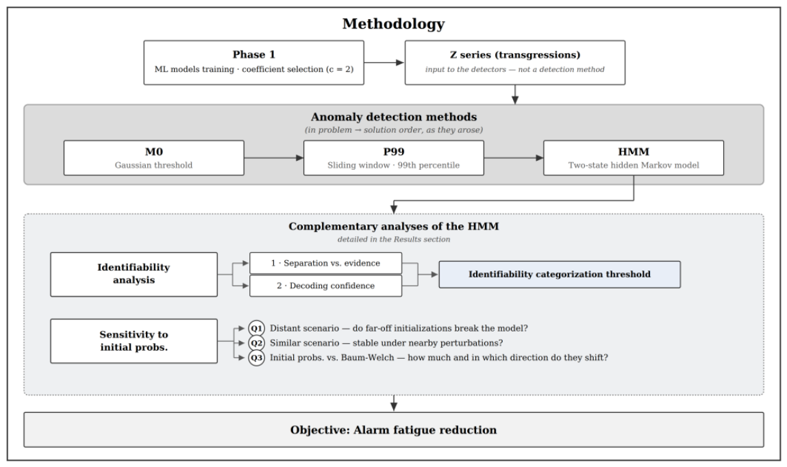
Figure 4.
Flagged sensors and flagged records by detection method (Z, M0, P99, HMM and their intersection “Both”, i.e. P99 ∩ HMM) for each dam. Columns correspond to dams and rows to metrics; labels give the percentage of sensors (top) and the mean per sensor across all/flagged sensors (bottom). Each panel has its own scale.
Figure 4.
Flagged sensors and flagged records by detection method (Z, M0, P99, HMM and their intersection “Both”, i.e. P99 ∩ HMM) for each dam. Columns correspond to dams and rows to metrics; labels give the percentage of sensors (top) and the mean per sensor across all/flagged sensors (bottom). Each panel has its own scale.
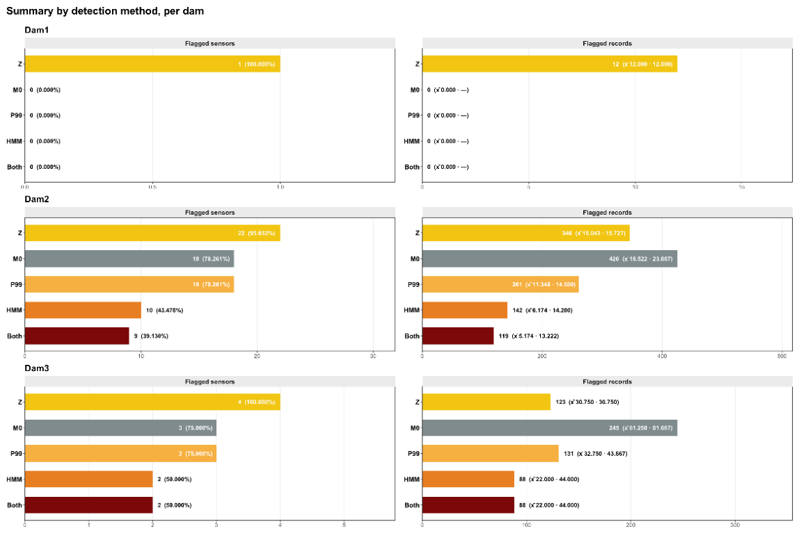
Figure 5.
Complete time series (training + validation) of pendulum P88098 (Dam2) with the M0 method. The target series is shown with the flagged periods shaded (proportion of transgressions in the window above the threshold).
Figure 5.
Complete time series (training + validation) of pendulum P88098 (Dam2) with the M0 method. The target series is shown with the flagged periods shaded (proportion of transgressions in the window above the threshold).
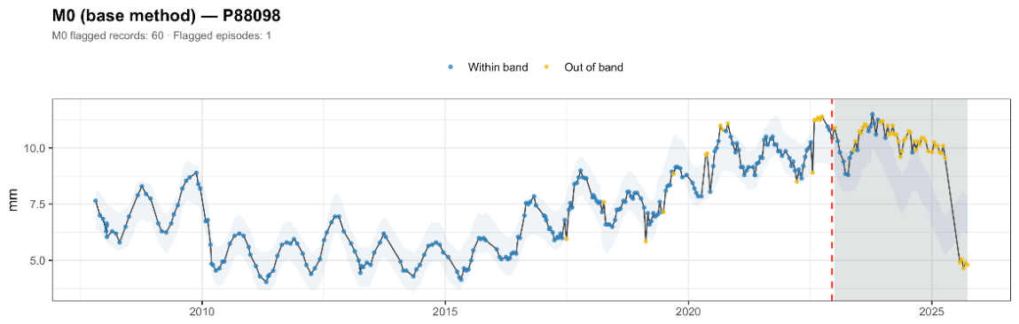
Figure 6.
Complete time series (training + validation) of pendulum P04626 (Dam2) with the P99 method. Points are coloured according to whether they fall inside or outside the prediction band (transgressions); the shaded band marks the duration of each P99 flagged streak and the vertical line its start.
Figure 6.
Complete time series (training + validation) of pendulum P04626 (Dam2) with the P99 method. Points are coloured according to whether they fall inside or outside the prediction band (transgressions); the shaded band marks the duration of each P99 flagged streak and the vertical line its start.
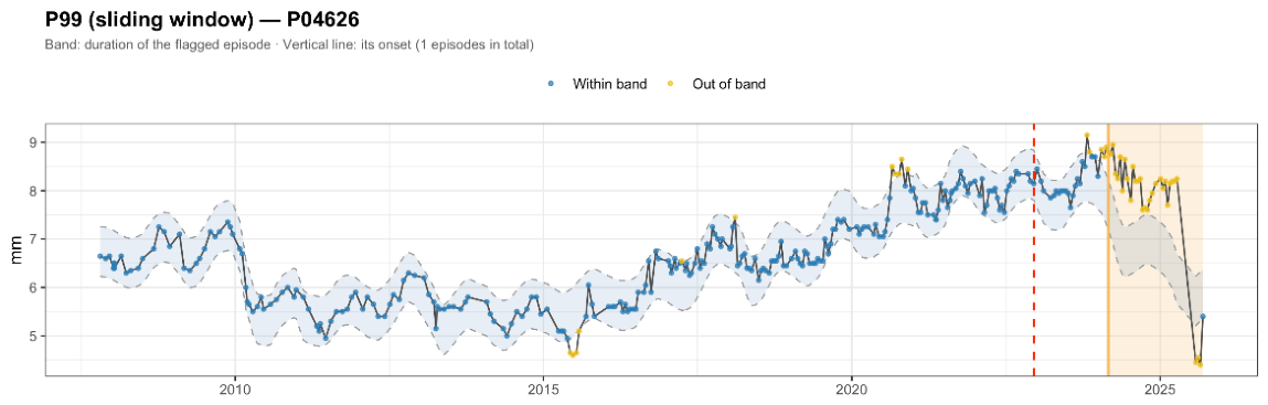
Figure 8.
Complete time series (training + validation) of pendulum P91039 (Dam1) with the states of the two-state HMM. The shading marks the anomalous state A: blue in training (period assumed free of structural problems) and red in validation (HMM flag); the red points are individual transgressions of the prediction band.
Figure 8.
Complete time series (training + validation) of pendulum P91039 (Dam1) with the states of the two-state HMM. The shading marks the anomalous state A: blue in training (period assumed free of structural problems) and red in validation (HMM flag); the red points are individual transgressions of the prediction band.
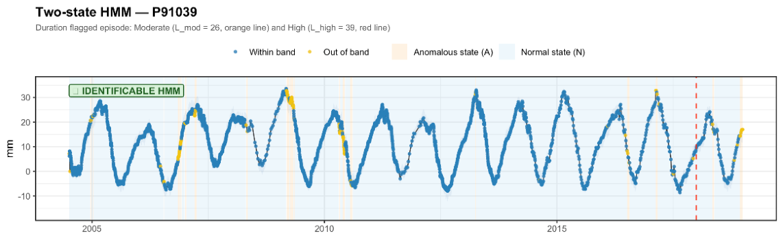
Figure 9.
Emission separation of the fit (ρ − ε) versus three descriptors of the transgression streaks in training, per sensor: (a) mean streak duration, (b) proportion of short streaks (≤2 records) followed by a long gap (≥3 records) and (c) maximum streak duration. The dashed line indicates the 0.22 threshold. Spearman rank correlations with the separation: +0.95 (a), −0.55 (b) and +0.87 (c).
Figure 9.
Emission separation of the fit (ρ − ε) versus three descriptors of the transgression streaks in training, per sensor: (a) mean streak duration, (b) proportion of short streaks (≤2 records) followed by a long gap (≥3 records) and (c) maximum streak duration. The dashed line indicates the 0.22 threshold. Spearman rank correlations with the separation: +0.95 (a), −0.55 (b) and +0.87 (c).
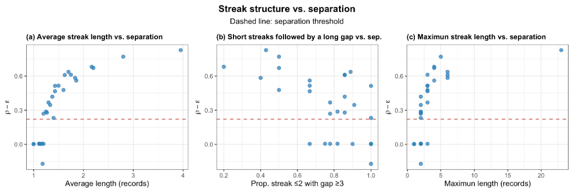
Figure 10.
Decoding confidence (mean posterior of the Anomalous state over the records with a transgression, Zt = 1) versus the emission separation, per sensor. The dotted line marks chance (0.5) and the dashed line the 0.22 threshold.
Figure 10.
Decoding confidence (mean posterior of the Anomalous state over the records with a transgression, Zt = 1) versus the emission separation, per sensor. The dotted line marks chance (0.5) and the dashed line the 0.22 threshold.
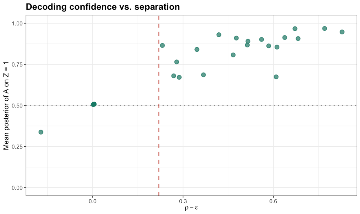
Figure 11.
Effect of the Baum-Welch initial probabilities on sensor P91039. Each panel corresponds to a different HMM initialisation —(a) reference, (b) low pAA, (c) low pNN and (d) high ε with low ρ— and shows the series with its prediction band (records in/out of band), the decoded state (normal/anomalous) and the flagged anomalous streaks; the label indicates whether the resulting fit is identifiable.
Figure 11.
Effect of the Baum-Welch initial probabilities on sensor P91039. Each panel corresponds to a different HMM initialisation —(a) reference, (b) low pAA, (c) low pNN and (d) high ε with low ρ— and shows the series with its prediction band (records in/out of band), the decoded state (normal/anomalous) and the flagged anomalous streaks; the label indicates whether the resulting fit is identifiable.
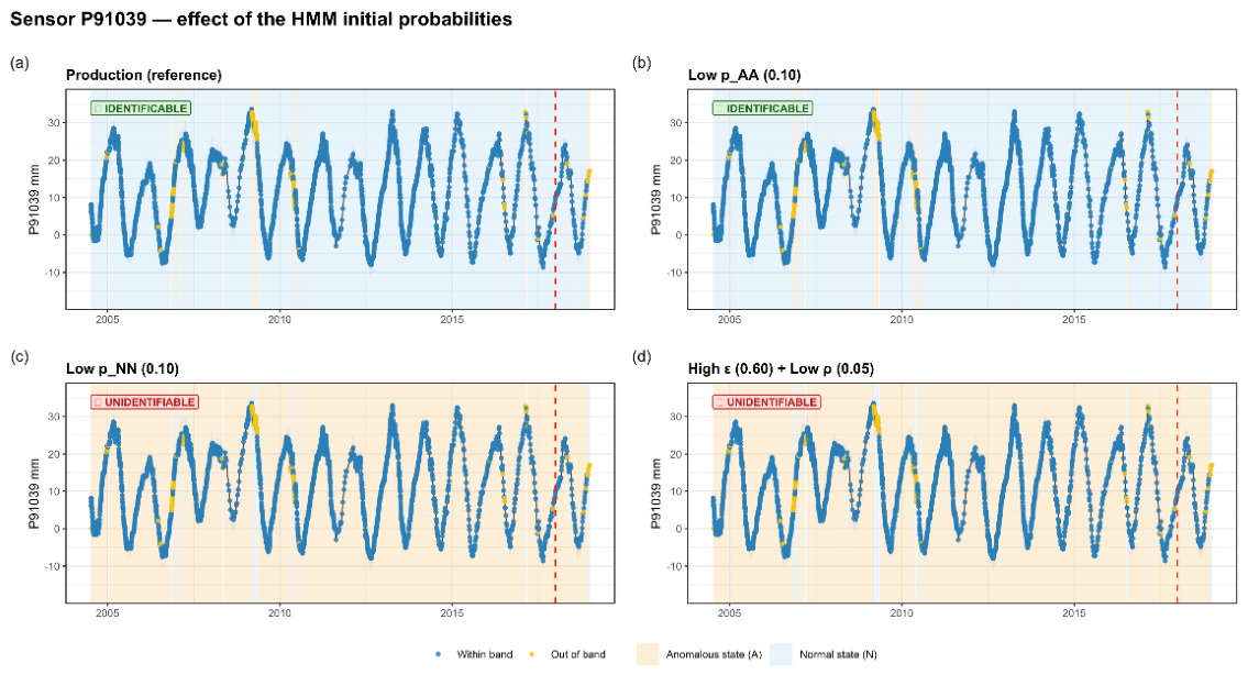
Figure 12.
Effect of the Baum-Welch initial probabilities on sensor P90710. Each panel corresponds to a different HMM initialisation —(a) reference, (b) low pAA, (c) low pNN and (d) high ε with low ρ— and shows the series with its prediction band (records in/out of band), the decoded state (normal/anomalous) and the flagged anomalous streaks; the label indicates whether the resulting fit is identifiable.
Figure 12.
Effect of the Baum-Welch initial probabilities on sensor P90710. Each panel corresponds to a different HMM initialisation —(a) reference, (b) low pAA, (c) low pNN and (d) high ε with low ρ— and shows the series with its prediction band (records in/out of band), the decoded state (normal/anomalous) and the flagged anomalous streaks; the label indicates whether the resulting fit is identifiable.
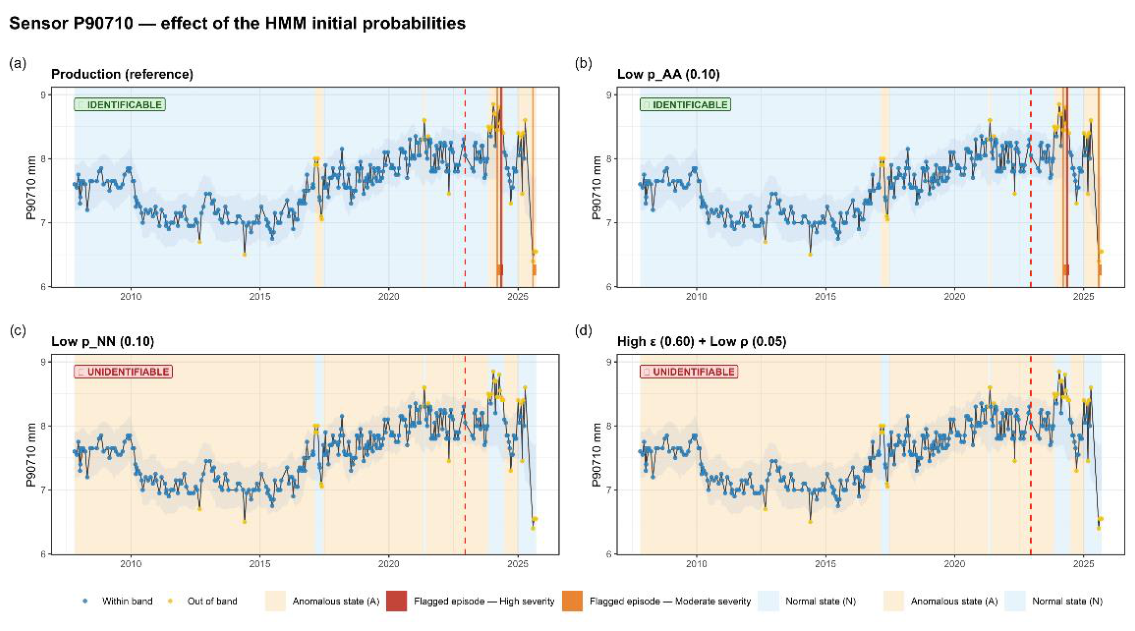
Figure 13.
Natural variation of the HMM final estimates across sensors. Each box summarises, for one parameter, the Baum-Welch estimates obtained with the reference initialisation over the identifiable sensors.
Figure 13.
Natural variation of the HMM final estimates across sensors. Each box summarises, for one parameter, the Baum-Welch estimates obtained with the reference initialisation over the identifiable sensors.
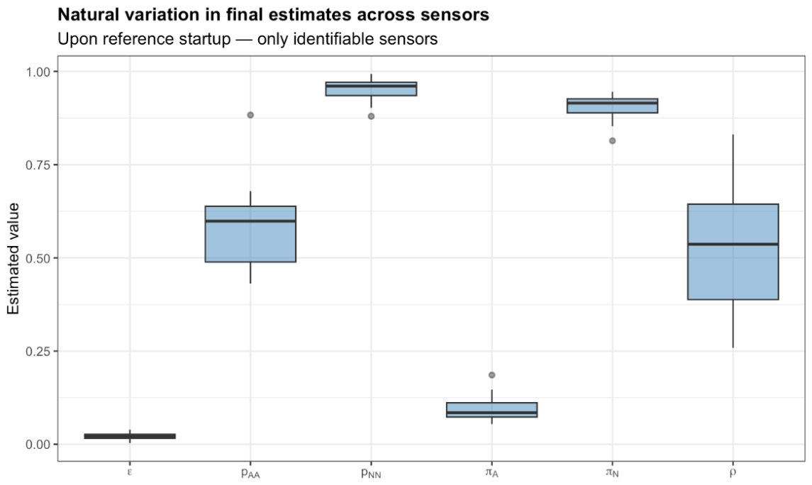
Figure 14.
Distant scenario: response of the HMM to the stress initialisations, by scenario. Left panel: distribution across sensors of the percentage of transgressions (Z = 1) that the HMM classifies in the Normal state (100 = total inversion). Right panel: percentage of sensors in which the scenario degenerates the HMM (non-identifiable). In both, colour groups the scenarios by category and “REF” is the reference initialisation.
Figure 14.
Distant scenario: response of the HMM to the stress initialisations, by scenario. Left panel: distribution across sensors of the percentage of transgressions (Z = 1) that the HMM classifies in the Normal state (100 = total inversion). Right panel: percentage of sensors in which the scenario degenerates the HMM (non-identifiable). In both, colour groups the scenarios by category and “REF” is the reference initialisation.
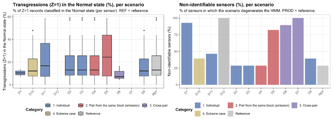
Figure 17.
Sweep of
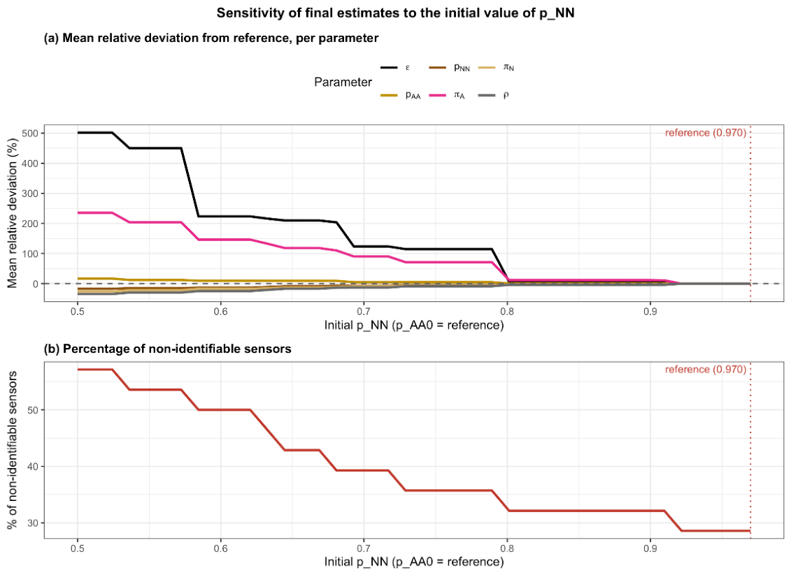
Table 1.
Main characteristics of the three dam cases. “Mean records per sensor” is the average number of readings per pendulum over the indicated period.
Table 1.
Main characteristics of the three dam cases. “Mean records per sensor” is the average number of readings per pendulum over the indicated period.
| Dam | Type | Height (m) | Target variable | Pendulums | Mean records per sensor | Date range |
| Dam1 | Arch-gravity | > 66 | Radial movement | 1 | 3589 | 2004-07-06 – 2018-12-30 |
| Dam2 | Gravity | 90.55 | Radial / tangential movement | 23 | 297 | 2007-10-24 – 2025-09-26 |
| Dam3 | Gravity | 45 | Radial / tangential movement | 4 | 353 | 2017-06-13 – 2026-02-10 |
Table 2.
Design of the Similar scenario experiments. In each experiment only one parameter block (transition, emission or initial state) is perturbed around its reference value, while the other two blocks are kept at their reference values.
Table 2.
Design of the Similar scenario experiments. In each experiment only one parameter block (transition, emission or initial state) is perturbed around its reference value, while the other two blocks are kept at their reference values.
| Experiment | Parameters that vary | Parameters kept at their reference values |
| Transition | The 16 combinations of and | ε(0),ρ(0),π(0) |
| Emission | Perturbations of ε(0) and ρ(0) | |
| Initial state | Perturbation of , with | |
Table 3.
Number and percentage of transgressions and of flags with the M0 method over the validation period of sensor P88098.
Table 3.
Number and percentage of transgressions and of flags with the M0 method over the validation period of sensor P88098.
| Num. Transgressions | Z=1 (%) | Num. M0 flagged records | M0 flagged records (%) |
| 44 | 73.3 | 60 | 100 |
Table 6.
Number and percentage of transgressions and of flags with the M0, P99 and HMM methods over the validation period of sensor P04626.
Table 6.
Number and percentage of transgressions and of flags with the M0, P99 and HMM methods over the validation period of sensor P04626.
| Num. Transgressions | Z=1 (%) | Num. M0 flagged records | M0 flagged records (%) | Num. P99 flagged records | P99 flagged records (%) | Num. HMM flagged records | HMM flagged records (%) |
| 36 | 62.1 | 32 | 55.2 | 32 | 55.2 | 26 | 44.8 |
Table 7.
Number and percentage of transgressions and of flags with the M0, P99 and HMM methods over the validation period of sensor P91039.
Table 7.
Number and percentage of transgressions and of flags with the M0, P99 and HMM methods over the validation period of sensor P91039.
| Num. Transgressions | Z=1 (%) | Num. M0 flagged records | M0 flagged records (%) | Num. P99 flagged records | P99 flagged records (%) | Num. HMM flagged records | HMM flagged records (%) |
| 12 | 11.5 | 0 | 0 | 0 | 0 | 0 | 0 |
Table 8.
Range of the final estimates across the 20 identifiable sensors (with the reference initial probabilities). Columns: parameter, minimum, maximum and absolute difference (max − min) across sensors.
Table 8.
Range of the final estimates across the 20 identifiable sensors (with the reference initial probabilities). Columns: parameter, minimum, maximum and absolute difference (max − min) across sensors.
| Parameter | Minimum | Maximum | Absolute difference |
| pNN | 0.880 | 0.993 | 0.114 |
| pAA | 0.431 | 0.883 | 0.452 |
| ε | 0.003 | 0.039 | 0.036 |
| ρ | 0.259 | 0.831 | 0.573 |
| πN | 0.814 | 0.946 | 0.132 |
| πA | 0.054 | 0.186 | 0.132 |
Table 10.
Similar scenario: deviation of the final estimates by perturbed block, aggregated across the 20 sensors identifiable with the reference initialisation.
Table 10.
Similar scenario: deviation of the final estimates by perturbed block, aggregated across the 20 sensors identifiable with the reference initialisation.
| Block (perturbed) | Parameter | Absolute Mean relative deviation (%) | Mean absolute deviation | Mean relative inter-range deviation (%) | Mean inter-range deviation |
| Emission (ε, ρ) | ε | 0.00 | 0.0000 | 0.00 | 0.0000 |
| Emission (ε, ρ) | pAA | 0.00 | 0.0000 | 0.00 | 0.0000 |
| Emission (ε, ρ) | pNN | 0.00 | 0.0000 | 0.00 | 0.0000 |
| Emission (ε, ρ) | πA | 0.00 | 0.0000 | 0.00 | 0.0000 |
| Emission (ε, ρ) | πN | 0.00 | 0.0000 | 0.00 | 0.0000 |
| Emission (ε, ρ) | ρ | 0.00 | 0.0000 | 0.00 | 0.0000 |
| Initial state (πN) | ε | 0.06 | 0.0000 | 0.18 | 0.0000 |
| Initial state (πN) | pAA | 0.06 | 0.0003 | 0.17 | 0.0009 |
| Initial state (πN) | pNN | 0.01 | 0.0001 | 0.03 | 0.0003 |
| Initial state (πN) | πA | 0.08 | 0.0001 | 0.24 | 0.0003 |
| Initial state (πN) | πN | 0.01 | 0.0001 | 0.04 | 0.0003 |
| Initial state (πN) | ρ | 0.10 | 0.0004 | 0.30 | 0.0012 |
| Transition (pNN, pAA) | ε | 38.92 | 0.0099 | 17.75 | 0.0540 |
| Transition (pNN, pAA) | pAA | 1.77 | 0.0088 | 5.59 | 0.0496 |
| Transition (pNN, pAA) | pNN | 2.82 | 0.0261 | 11.38 | 0.1052 |
| Transition (pNN, pAA) | πA | 29.57 | 0.0298 | 19.38 | 0.1339 |
| Transition (pNN, pAA) | πN | 3.36 | 0.0298 | 15.10 | 0.1339 |
| Transition (pNN, pAA) | ρ | 5.12 | 0.0191 | 20.80 | 0.0795 |
Table 11.
Sensors appearing as outliers in the “with outliers” boxplot above. Columns: parameter, sensor, relative deviation (%) and whether that sensor ceases to be identifiable with
Table 11.
Sensors appearing as outliers in the “with outliers” boxplot above. Columns: parameter, sensor, relative deviation (%) and whether that sensor ceases to be identifiable with
| Parameter | Sensor | Deviation (%) | Identifiability |
| epsilon | P28558 | 2176.483 | FALSE |
| epsilon | P76702 | 119.069 | FALSE |
| epsilon | P91942 | 177.016 | FALSE |
| p_AA | P28558 | 86.257 | FALSE |
| p_AA | P76702 | 14.641 | FALSE |
| pi_A | P28558 | 1182.371 | FALSE |
| pi_A | P76702 | 237.195 | FALSE |
| pi_A | P91942 | 382.259 | FALSE |
Disclaimer/Publisher’s Note: The statements, opinions and data contained in all publications are solely those of the individual author(s) and contributor(s) and not of MDPI and/or the editor(s). MDPI and/or the editor(s) disclaim responsibility for any injury to people or property resulting from any ideas, methods, instructions or products referred to in the content. |
© 2026 by the authors. Licensee MDPI, Basel, Switzerland. This article is an open access article distributed under the terms and conditions of the Creative Commons Attribution (CC BY) license (http://creativecommons.org/licenses/by/4.0/).
Copyright: This open access article is published under a Creative Commons CC BY 4.0 license, which permit the free download, distribution, and reuse, provided that the author and preprint are cited in any reuse.