

Submitted:
08 October 2026
Posted:
09 October 2026
Read the latest preprint version here
Abstract
SAE J2597 tests whether saturation-curve software reproduces reference intensities. That shows computational conformance. It does not show that an individual Almen result is fit to report. This paper proposes four conditions for result eligibility: method qualification, measurement integrity, exposure support and adequacy. We test them on the ten J2597 datasets, on a 388-strip replicated experiment and in simulation. All three J2597 example equations meet the targets, yet they differ in intensity by up to 0.0012 in. Strip-lot effects scale intensity but leave characteristic exposure unchanged, so checks apply within one lot. A gamma mixture of exponential rates, GAM3, contains two J2597 equations as limits and reaches all ten targets within 0.00006 in. In simulation, fixing its shape parameter from a qualification curve cuts the error in characteristic exposure from about 10% to 4%. The saturation curve can be read as a work-hardening law of the impacted layer, an analogy of form. A frozen qualification curve, with verification strips at the exposures where each fault shows, detects drifts that single-strip verification misses. Seventeen provisions are proposed. All thresholds are candidates that need locked implementation and independent validation before use in a standard.
Keywords:
Almen strip
; saturation curve
; characteristic exposure
; nonlinear regression
; model-form sensitivity
; result reporting
1. Introduction
1.1. The problem
Shot-peening intensity is measured with Almen strips. Strips are peened for a series of exposures, and the arc height of each is measured. The arc height rises with exposure and then saturates. The plot of arc height against exposure is the saturation curve.
J443 defines the intensity, IA, as the arc height at the exposure TA at which doubling the exposure raises the arc height by 10%. This is the Almen 10% rule. In the notation of Table 1, IA = hA(TA), where RA(TA) = 0.10 and RA is the fractional rise in arc height when the exposure doubles.
1.2. The Three Equations in J2597
J2597 does not prescribe an equation. It gives three example algorithms. For four-point data it recommends the two-parameter exponential, EXP2. For data with more than four points it recommends the three-parameter exponential, EXP3. Where NF L 06-832 applies, it gives the two-parameter saturation-growth form, HYP2. The three forms are:
EXP2: hA(E) = a[1 − exp(−bE)]
EXP3: hA(E) = a[1 − exp(−b′Ec)]
HYP2: hA(E) = aE / (b + E)
Here E is exposure and hA is the fitted arc height. The parameter a is the asymptotic arc height. The parameters b, b′ and c set the rate and the shape. In J2597 they are Equation 1 (EXP2), Equation 3 (EXP3) and Equation 2 (HYP2).
1.3. The Gap
Reproducing ten reference curves shows that a program calculates correctly. It does not show that an individual strip result is fit to report. J2597 says so itself. Its Caution (Section 3.1) leaves the user to validate data and results independently of the program.
Three things can still go wrong. The strips may carry errors that no curve fit can see. The exposures may not support the 10% point. And the choice of equation may move the answer. All three J2597 equations meet the targets, yet they differ by up to 0.0012 in on one dataset (Section 4.1).
1.4. Earlier Work
Kirk found that programs agree more closely on intensity than on characteristic exposure. He discussed satisfactory curve shape, advised matching equation complexity to the number of observations, and stressed the placement of exposures [2,3,5,6,7]. He also documented three further effects. The exposure range changes the fitted result. The J443 definition of intensity changed between 1952 and 2010, and the earlier wording was ambiguous. The Almen gauge itself is a source of error [8,9,10,11].
Bailey et al. and Champaigne reported differences between strip suppliers, and between strips that meet every J442 attribute [12,13]. The regression, calibration and metrology literature separates numerical verification, model discrepancy, measurement uncertainty, identifiability and decision thresholds [14,15,16,17].
This paper does not discover these effects. It turns them into explicit, testable reporting rules.
1.5. This Paper
We propose four conditions that a result must meet before it is reported. The method is qualified. The measurement is sound. The exposures support the characteristic point. And the reported intensity does not depend materially on the equation chosen. We call these method, measurement, support and declared family (Table 2). Together they define eligibility for reporting under the declared procedure.
We test the conditions on the ten J2597 datasets, on Wieland’s replicated experiment of 388 strips and on simulation. We derive a reporting equation, GAM3, from the spread of local rates on the strip. We read the saturation curve as a work-hardening curve of the impacted layer and give a procedure for generating and verifying curves. We propose seventeen provisions.
Here qualification applies to the calculation method or to an individual result. It never means qualification of the production process.
The evidence is exploratory. Thresholds and fixtures were developed on the same data used to illustrate them. We report mathematical results, data illustrations, simulations and standards implications separately, and infer no sensitivity, specificity, false-release probability or field prevalence.
Section 2 gives the methods, Section 3 four analytical results and Section 4 the results from data and simulation. Section 5 and Section 6 give the limits and conclusions. The appendices hold the provisions, fixtures, simulation specifications, Wieland data and fitting settings.
Some figure labels keep and as compact shorthand for and . The prose, equations and decision statements use Table 1.
The standards baseline used here is SAE J442_202602, J443_202512, J2597_201709 and J2277_202301, together with AMS2430U, AMS2432E and AMS2431E [1,18,19,20,21,22,23]. We read controlled copies of all of them, and clause-level statements rest on those copies.
Conventions. Arc height and intensity follow the designation in SAE J443: the value in inches, then the unit and the Almen strip type, for example 0.0126 in A. Where a source reported metric values, the original is given in parentheses, for example 0.012 in A (0.30 mm A). Differences, tolerances and standard deviations of arc height are given in inches without a strip type.
2. Methods
2.1. Study Design and Evidentiary Categories
This is a framework-development study with internal stress testing. We kept four forms of evidence distinct: analytical results that follow from specified equations or error mechanisms; numerical illustrations using published J2597 reference data; secondary analysis and resampling of Wieland’s historical single-system experiment; and simulations generated under explicit distributions chosen by the author. We treat proposed standards language as a research output, not as a finding or a ready specification.
Cases were not held out. Two implementations were written by the same author; their agreement is an implementation check, not independent scientific replication.
2.2. Candidate Framework and Decision Semantics
The framework represents the decision that a result is eligible for reporting under the declared procedure as the conjunction of four declared conditions:
Passing these checks means only that the calculated Almen result is eligible for reporting under the declared procedure. They do not qualify the production process, prove that the physical response is correct, exclude all relevant faults or imply an engineering outcome. A status of model sensitive refers only to the declared comparison family.
2.3. Curve Definitions and Fitting
Let denote the fitted Almen response at exposure . The Almen fractional doubling increment , characteristic exposure and reported intensity are defined by;
TA is the earliest positive solution of RA(E) = 0.10 in the search domain. Curves are fitted by unweighted least squares. The reporting equation is EXP2 for a four-point set and EXP3 for a six-point set. HYP2 is kept only for comparison. A failed fit is a non-release outcome. The fitting settings must be locked before external evaluation. Bounds, starting values and root-search settings are in Appendix E.
2.4. Data Sources
Table 3 lists the sources and what each supplies. We read controlled copies of the standards, and the data, targets and clauses of J2597_201709 were checked against the copy held by SAE Mobilus (accessed 4 October 2026).
The canonical benchmark applies PCHIP to the full-precision exposure means and solves , giving s and in. A local linear interpolation between the 60/120 s and 70/140 s doubling pairs is a transparent sensitivity calculation and gives 66.9 s and 0.01261 in A. The reported 5,000-sample interval of 65.6–68.2 s was generated by within-exposure linear-interpolation resampling and is not a PCHIP interval. Both benchmarks exclude model, grid, machine, day, operator, gauge and complete process uncertainty.
2.5. Internal Stress Testing
Fourteen matched accept and reject fixtures exercise exposure support, first-point placement, residual behaviour, a decreasing final observation, a nearly degenerate response, and sensitivity to a gap between exposures. Their intended labels were set by the author. They are acceptance-test fixtures for implementation, not independent falsification evidence. Full point data are in Appendix B.
The provisional values are = 0.00016 in, = 3.5, in, and . None is proposed as a validated operating threshold. The comparison statistic was calculated over a declared admissible set rather than over every fitted equation, where P3–P5 are the characteristic-point, support and fit-adequacy checks of Appendix A:
2.6. Conditional Simulations and Estimands
The one-million-curve exercise drew individual readings with replacement from Wieland’s exposure-specific observations, selected four to six exposures from the 15 available, rounded readings to 0.0001 in, and imposed the specified pre-bow scenarios. Additional synthetic studies used exponential and hyperbolic truth models with Wieland-like scatter. Full boundaries are in Appendix C.
The estimand is the conditional frequency of each decision and error category among curves generated by the stated resampling, exposure-selection, fitting, and error model. It is not the frequency of errors in industrial practice, the probability that current software is unsafe, or the operating performance of the framework across laboratories.
2.7. Statistical Analysis
Unweighted least squares, case-deletion refitting, point perturbations, within-exposure resampling [25] and replicated lack-of-fit tests were used. The Appendix B audit applies the declared EXP2 four-point and EXP3 six-point reporting rule to the stored numerical results. Raw per-curve files and executable code are not yet archived, so the million-curve results have not been independently recomputed. The Wieland benchmark, the lack-of-fit statistics and the Appendix B margins were recomputed from the Appendix D readings and the Appendix B point data and agree with the values reported.
Cross-validation. Each exposure level, or each point of a six-point reference set, was withheld in turn. The equation was refitted to the remaining points and used to predict the withheld one. The cross-validated RMSE is the root mean square of these prediction errors.
3. Analytical Results Under Stated Curve and Error Models
Table 4 states the scope of each result. The results show properties of specified equations or error mechanisms, not the prevalence of failures in production.
3.1. Result 1 Crossing Behaviour Imposed by EXP2 and HYP2
Substitution into Equation (5) gives for EXP2 and = b/(b + 2E) for HYP2. Both are strictly decreasing for positive and positive parameters. Their dimensionless slopes at the 10% point are and at , respectively. A unique downward crossing is therefore guaranteed by model form. It is not independent evidence that the observed physical response has saturated.
3.2. Result 2 Local Geometric Sensitivity Near the Characteristic Point
For a small displacement evaluated along a fitted curve, . The corresponding local conversion is
For EXP2, = 9/ln(10) ≈ 3.9; for HYP2, . This is a local geometric sensitivity along each fitted curve. It is not an estimator condition number: it ignores parameter covariance, observation design, correlated errors, weighting and model misspecification.
3.3. Result 3 Finite Point Agreement Under Flexible Alternatives
For an unrestricted sufficiently flexible alternative, add to a fitted curve, where
The perturbation vanishes at the origin, every measured exposure , , and , while its derivative at need not vanish. It can therefore alter the number or direction of crossings without altering the checked values. This is an impossibility result for finite observations under an unrestricted flexible alternative. Smoothness, monotonicity, curvature, measurement resolution, or a physically justified response class can weaken or exclude the construction.
3.4. Result 4 Conditional Common-Offset Mechanism
If a positive offset is added to every arc height, the numerator of is unchanged and the denominator increases:
For decreasing , the 10% point moves to an earlier exposure, and the reported intensity does not simply increase by . This establishes a mathematical mechanism. Whether pre-bow, mounting, thickness, hardness or gauge practice produces such an offset is an empirical question.
4. Results
4.1. Historical Reference Data Illustration
Both two-parameter equations reproduced all ten reference targets within the in allowance stated for J2597_201709 [1]. Their largest between-equation intensity difference was 0.00090 in for Set 6. In that case HYP2 also placed beyond the longest measured exposure. This shows model dependence. It does not show that either model is physically incorrect. Re-fitting all ten datasets from the controlled copy confirms this and extends it to EXP3: all three equations reach every target, with largest deviations of +0.00028 in for EXP2 (Set 8), +0.00090 in for HYP2 (Set 6) and -0.00029 in for EXP3 (Set 6) (Supplementary Data S4; Table 6 and Table 7). Three admissible equations therefore give intensities spread by up to 0.0012 in on one dataset while all comply.

Table 5.
EXP2 and HYP2 fits to the ten J2597 reference datasets.
| Set | n | Target IA | EXP2 IA | EXP2 TA | HYP2 IA | HYP2 TA | EXP2 dev (in) | HYP2 dev (in) | HYP2 2TA supported |
|---|---|---|---|---|---|---|---|---|---|
| 1 | 4 | 0.0064 | 0.006410 | 4.754 | 0.006392 | 4.755 | +0.00001 | −0.00001 | Yes |
| 2 | 4 | 0.0040 | 0.003939 | 5.478 | 0.003978 | 7.055 | −0.00006 | −0.00002 | Yes |
| 3 | 4 | 0.0080 | 0.008008 | 5.382 | 0.007929 | 6.167 | +0.00001 | −0.00007 | Yes |
| 4 | 4 | 0.0048 | 0.004833 | 1.805 | 0.005093 | 2.617 | +0.00003 | +0.00029 | No |
| 5 | 4 | 0.0066 | 0.006572 | 4.730 | 0.006553 | 4.730 | −0.00003 | −0.00005 | Yes |
| 6 | 4 | 0.0098 | 0.009804 | 3.902 | 0.010703 | 6.901 | +0.00000 | +0.00090 | No |
| 7 | 4 | 0.0063 | 0.006249 | 2.756 | 0.006423 | 3.356 | −0.00005 | +0.00012 | No |
| 8 | 6 | 0.0093 | 0.009582 | 0.433 | 0.009372 | 0.466 | +0.00028 | +0.00007 | Yes |
| 9 | 6 | 0.0137 | 0.013770 | 0.546 | 0.013712 | 0.663 | +0.00007 | +0.00001 | Yes |
| 10 | 6 | 0.0054 | 0.005494 | 0.463 | 0.005382 | 0.502 | +0.00009 | −0.00002 | Yes |
Table 6.
Deviation of fitted intensity from each J2597 target, for the three example equations (in), with the largest spread between them on each dataset.
Table 6.
Deviation of fitted intensity from each J2597 target, for the three example equations (in), with the largest spread between them on each dataset.
| Set | Observations | EXP2 | HYP2 | EXP3 | Largest spread between equations |
|---|---|---|---|---|---|
| 1 | 4 | +0.00001 | −0.00001 | −0.00004 | 0.00004 |
| 2 | 4 | −0.00006 | −0.00002 | −0.00003 | 0.00004 |
| 3 | 4 | +0.00001 | −0.00007 | +0.00001 | 0.00008 |
| 4 | 4 | +0.00003 | +0.00029 | −0.00003 | 0.00032 |
| 5 | 4 | −0.00003 | −0.00005 | −0.00005 | 0.00002 |
| 6 | 4 | 0.00000 | +0.00090 | −0.00029 | 0.00119 |
| 7 | 4 | −0.00005 | +0.00013 | −0.00016 | 0.00028 |
| 8 | 6 | +0.00028 | +0.00007 | +0.00012 | 0.00021 |
| 9 | 6 | +0.00007 | +0.00001 | +0.00024 | 0.00022 |
| 10 | 6 | +0.00009 | −0.00002 | +0.00007 | 0.00011 |
Table 7.
Summary of each equation’s fit to the ten J2597 reference datasets.
| Equation | Datasets within ±0.0010 in | Largest deviation (in) | Mean absolute deviation (in) | RMS deviation (in) | Datasets where 2TA lies beyond the longest exposure |
|---|---|---|---|---|---|
| EXP2 | 10 of 10 | +0.00028 (Set 8) | 0.00006 | 0.00010 | none |
| HYP2 | 10 of 10 | +0.00090 (Set 6) | 0.00016 | 0.00030 | 3 of 10 (Sets 4, 6, 7) |
| EXP3 | 10 of 10 | −0.00029 (Set 6) | 0.00010 | 0.00014 | none |
Figure 1.
Deviation from each J2597 target as a fraction of the in allowance stated in J2597_201709 [1]. Daggers identify cases in which HYP2 placed beyond the largest measured exposure. The comparison is conditional on these two fitted equations; graphic labels use as shorthand for .
Figure 1.
Deviation from each J2597 target as a fraction of the in allowance stated in J2597_201709 [1]. Daggers identify cases in which HYP2 placed beyond the largest measured exposure. The comparison is conditional on these two fitted equations; graphic labels use as shorthand for .
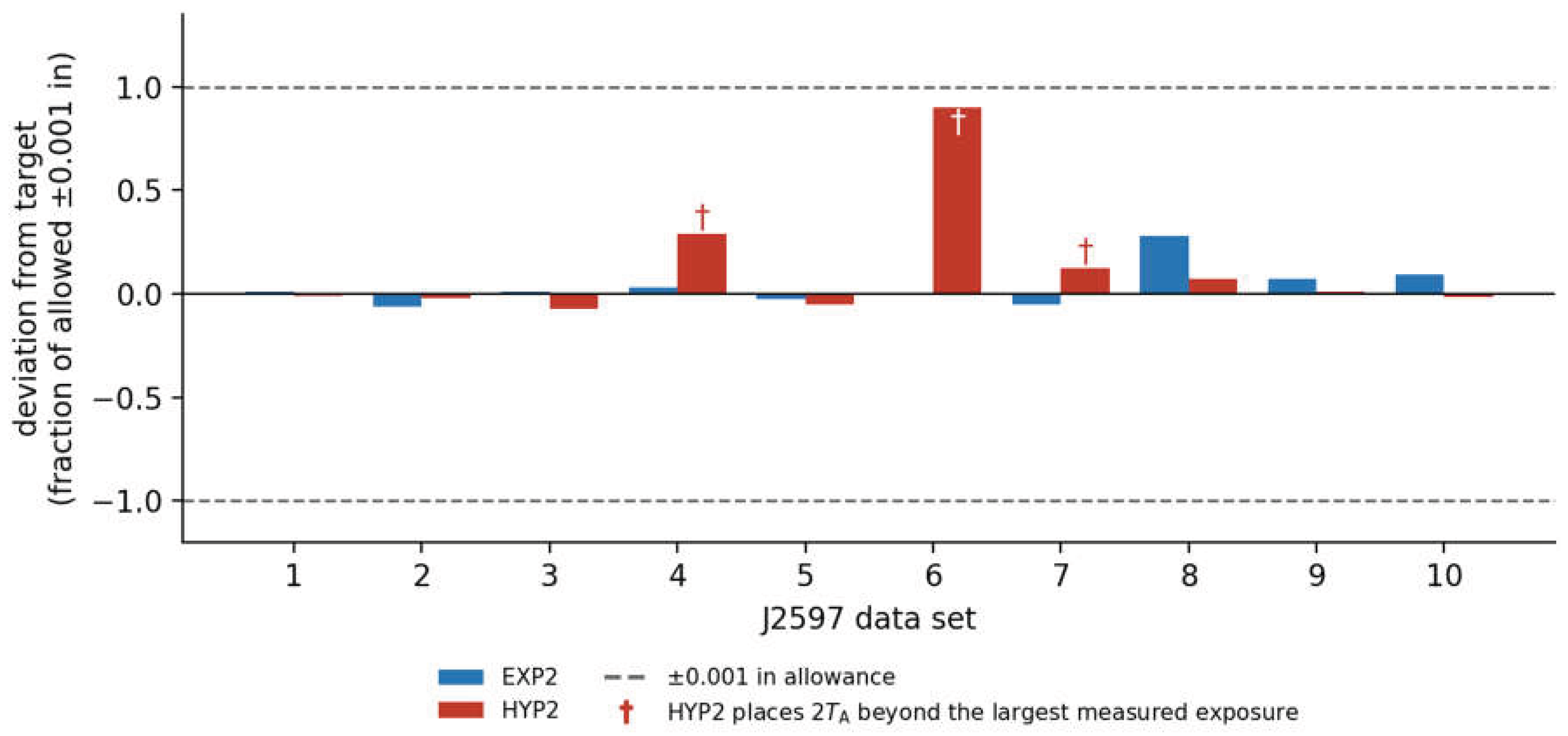
Table 6 gives the deviation from each target dataset by dataset, and Table 7 summarises each equation. Every equation reaches every target. The spread between the three equations is largest for Set 6, where HYP2 is +0.00090 in from the target and EXP3 is −0.00029 in from it, a spread of 0.00119 in.
Case-deletion refitting, with each observation deleted in turn, was used as a fragility diagnostic, not as a prediction interval. EXP2 remained within the stated allowance for every deletion. HYP2 did so for nine datasets; for Set 6, deletion of the longest exposure moved intensity 0.00199 in and placed it 0.00289 in above target. Perturbing one reading by in changed intensity by at most 0.00007 in for EXP2 and 0.00012 in for HYP2. At in, the corresponding maxima were 0.00036 and 0.00064 in. In this limited analysis, the longest exposure was the most influential point for every dataset and equation. Table 8 summarises these checks.
4.2. Historical Replicated Experiment
Across Wieland’s exposures, sample standard deviations ranged from 0.00012 to 0.00021 in; the pooled value was 0.00016 in over 373 degrees of freedom. The source analysis found no within-exposure drift with sample order (pooled Spearman , p = 0.44). These quantities describe one historical experimental system.
Figure 2.
Wieland’s 388 historical readings, exposure means, three fitted equations and the interpolation benchmarks. The displayed interval is conditional on the observed grid and the linear-interpolation resampling rule. EXP2 and EXP3 lie close to both empirical intensity estimates; HYP2 places characteristic exposure later.
Figure 2.
Wieland’s 388 historical readings, exposure means, three fitted equations and the interpolation benchmarks. The displayed interval is conditional on the observed grid and the linear-interpolation resampling rule. EXP2 and EXP3 lie close to both empirical intensity estimates; HYP2 places characteristic exposure later.
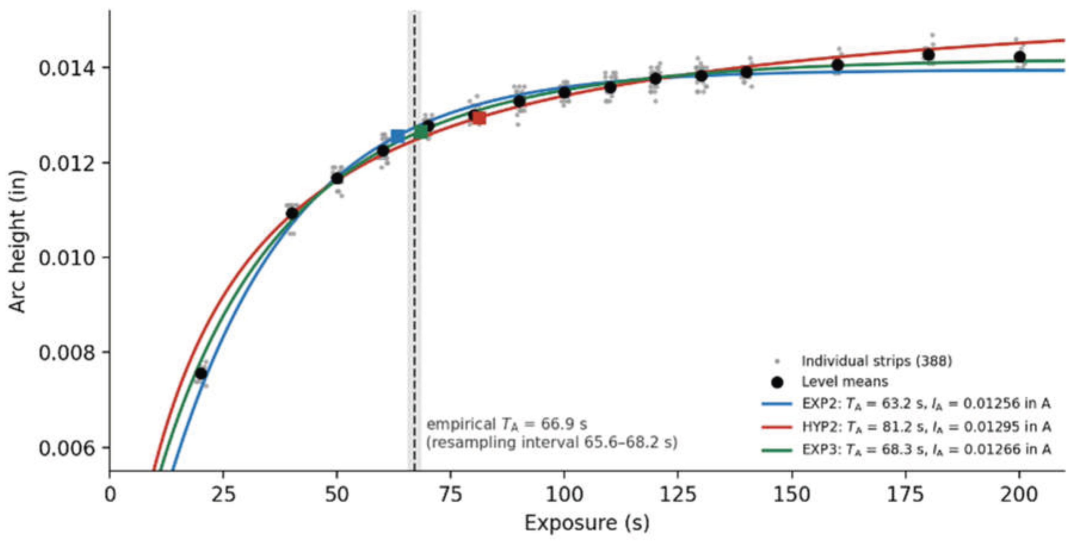
Relative to the canonical PCHIP benchmark in at s, EXP2 reported in A and s; EXP3 reported in A and s; and HYP2 reported in A and s. The linear-interpolation benchmark is 0.01261 in A at 66.9 s. The fitted intensities remain close to either benchmark while differs more materially. Replicated lack-of-fit tests rejected exact equality between each curve and the exposure means: F = 28.1 for EXP2 and 29.3 for HYP2 on (13, 373) degrees of freedom, and 8.8 for EXP3 on (12, 373), all . Statistical detectability of small discrepancy is not equivalent to engineering inadequacy of the inferred intensity.
4.3. Internal Stress Testing of Candidate Checks
Under the declared reporting rule, thirteen fixtures take their intended labels. C1-A needs explanation. EXP2 is the four-point reporting equation and passes P4 for C1-A, but HYP2 places at 1.19 times the last exposure and is inadmissible. Equation (6) therefore leaves one member in the admissible set, so C1-A is MODEL SENSITIVITY: NOT ASSESSABLE and is not eligible for reporting. For C5-R, EXP3 converges to a nearly degenerate fit with amplitude a ≈ 0.147 in and b′ at the lower bound; the NON SATURATION RESPONSE classification is therefore conditional on the declared bounds and must be reassessed if they change.
Under the locked reporting rule, four-point Sets 1–7 use EXP2 and six-point Sets 8–10 use EXP3. Sets 8 and 9 are eligible under EXP3; their largest residuals are 0.00019 and 0.00014 in, respectively. Under EXP2 they would fail the provisional 3.5u limit at 4.1u and 6.9u. Nine of the ten reference datasets are eligible for reporting under the declared procedure. Set 6 is MODEL INADEQUATE at 3.8u under the provisional limit and would pass at = 3.9. The classification of Set 6 therefore depends on the provisional limit, and no threshold in this paper has been set by an analysis of the costs of a wrong decision.
4.4. Conditional Simulation Results
In the one-million-curve development simulation, the candidate checks reduced large errors among results eligible for reporting under the declared procedure under the specified Wieland resampling and error scenarios. For flat or signed-corrected strips, the source analysis reported no eligible result outside the in J2597 allowance. Among 355,182 flat-strip results eligible across three equations, the largest absolute intensity error was 0.00093 in.
The checks also held many curves whose simulated intensity happened to be within 0.0005 in of the benchmark. Across randomly drawn exposure designs, approximately 25–30% of curves were held, largely for insufficient support. When the series was planned to span to in the development simulation, the share of within-tolerance curves held fell from 25% to 8% for EXP2 and from 26% to 12% for EXP3. These results motivate prospective study of exposure design.
Figure 3.
Conditional percentage of four-strip results eligible for reporting under the declared procedure with more than 10% from the stipulated truth for three response shapes. The frequencies arise from the source simulation model and do not estimate industrial prevalence. Confirmation pairs improve the conditional result at the cost of additional strips and repeated bracketing; graphic labels use as shorthand for .
Figure 3.
Conditional percentage of four-strip results eligible for reporting under the declared procedure with more than 10% from the stipulated truth for three response shapes. The frequencies arise from the source simulation model and do not estimate industrial prevalence. Confirmation pairs improve the conditional result at the cost of additional strips and repeated bracketing; graphic labels use as shorthand for .
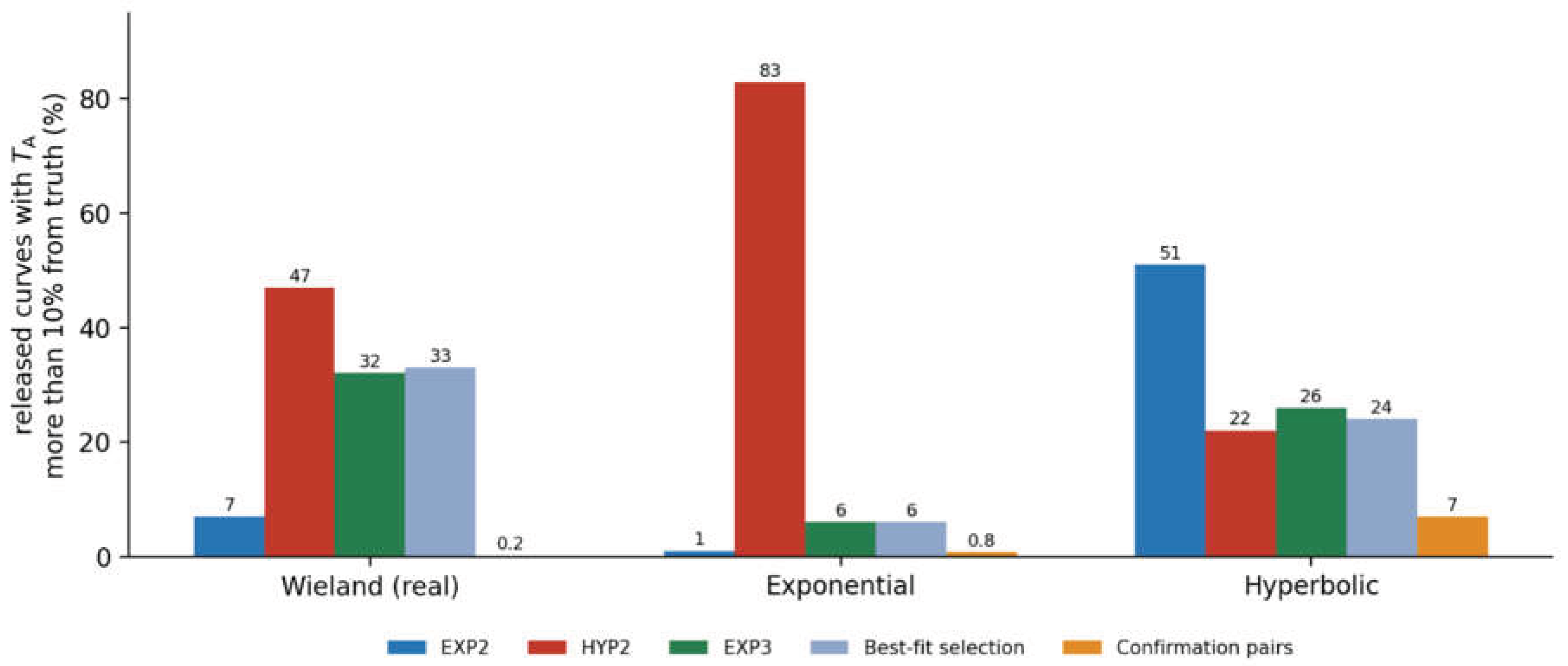
Characteristic exposure remained more model- and design-sensitive than intensity. Under the three simulated truth shapes, intensities eligible for reporting under the declared procedure were more than 0.0005 in from truth in at most 2.3% of curves, whereas corresponding values were more than 10% from truth in up to 83%. A matching equation was still imprecise with four single strips.
4.5. Common-Offset Mechanism and Pre-Bow Scenarios
The source simulations then imposed signed, unsigned, random-orientation, and lot-biased pre-bow scenarios. Under those assumptions, signed correction reproduced flat-strip behaviour, while a consistent +0.0010 in lot offset passed the curve-internal checks and shifted reported intensities by approximately 0.00091–0.00097 in. These results do not show that pre-bow acts as a constant offset in practice or how often a lot has a consistent sign.
Figure 4.
Mathematical common-offset illustration using Wieland’s exposure means and EXP2. Adding 0.0010 in lowers the fractional doubling increment, moves fitted from approximately 63 to 59 s, and raises fitted by approximately 0.00085 in. The figure demonstrates the stipulated additive mechanism, not its prevalence in production; graphic labels use as shorthand for .
Figure 4.
Mathematical common-offset illustration using Wieland’s exposure means and EXP2. Adding 0.0010 in lowers the fractional doubling increment, moves fitted from approximately 63 to 59 s, and raises fitted by approximately 0.00085 in. The figure demonstrates the stipulated additive mechanism, not its prevalence in production; graphic labels use as shorthand for .
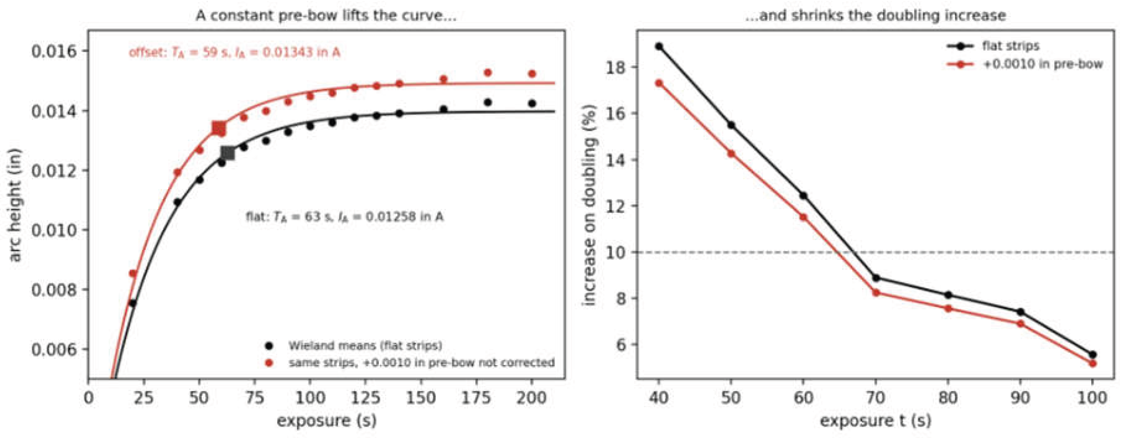
No clause-level claim is made here about mandatory signed correction, lot-mean limits or orientation-recording practice. A direct experiment with characterised signed pre-bow, controlled peening, several lots, orientations and gauges is needed first.
4.6. Multiplicative Lot Effects and Mixed-Lot Records
Pre-bow is one lot-dependent strip property; thickness and hardness are others. Within J442 tolerances the A-strip thickness may vary by about and hardness across 44–50 HRC. Under elastic bending, arc height scales approximately as the inverse square of thickness, so thickness alone could change arc heights at fixed exposure by about . Unlike pre-bow, such properties multiply the whole response. A lot factor, , was therefore applied to the canonical dataset and compared with the additive offset of Section 4.5 (Supplementary S1, which reproduces the fits of EXP2, HYP2 and EXP3 to the 388 readings).
For all three equations, scaling every reading by 0.95 or 1.05 changed by exactly −5.0% or +5.0% and left unchanged, because depends only on the rate and shape parameters. A +0.0010 in offset, the J442 maximum pre-bow, instead moved both quantities (Table 9). A change in at unchanged therefore indicates a multiplicative strip property such as thickness, whereas a change in indicates an additive or shape effect such as pre-bow or residual stress from strip manufacture.
Mixing lots also changes the lack-of-fit test, whose pure-error term assumes one lot. If each exposure level contained strips from two lots differing by , the median within-level standard deviation would rise from 0.00016 to 0.00037 in. The F statistics for EXP2, HYP2 and EXP3 would fall from 28.0, 29.3 and 8.7 to 5.4, 5.6 and 1.7. EXP3 would then no longer be rejected at the 5% level : mixing lots within exposure levels hides model inadequacy. If instead lot changed with exposure, as in the step scenario of Table 9, the F statistics rose to 100, 35 and 36 and was biased by 11–24 s, so a lot change produces both a false lack-of-fit signal and a real bias.
Monte Carlo four-strip curves (4000 per case, EXP2 reporting fit, the fitted EXP3 response as truth and Wieland within-lot scatter) show two regimes. When all four strips share one lot, a between-lot coefficient of variation of 2% or 4% sets a floor of 2.1% or 4.1% on the coefficient of variation of that additional strips cannot remove, while stays at 1.8 s for the 20-40-160-180 s design. When each strip comes from a different lot, the lot effect acts as extra noise: rises to 2.9 s and 5.0 s for that design, and from 3.2 s to 5.7 s and 9.9 s for a 40-60-80-120 s design. A lot of the kind reported by Champaigne, modelled as half the strips reading 8% low, tripled to 5.3 s and lowered mean by about 4%.
Consequence. The eligibility checks and standard errors of this paper apply within one strip lot. A record that combines lots, or does not identify the lot, cannot be assessed against them. Two candidate provisions follow (Appendix A, P11 and P12). Each saturation curve should be built from a single recorded lot. A lot-response qualification should estimate the between-lot variance: a sample from each lot is peened at one reference condition and compared with a reference lot. A single lot is necessary for this variance model but not sufficient for a valid measurement, which also needs independent strips, a stable gauge and no systematic variation within the lot.
4.7. Robustness of the Lack-of-Fit Test to Its Assumptions
The F-ratio lack-of-fit test was simulated under five error models (Supplementary Data S2 and S8). Its size stays between 3.5% and 6% at a nominal 5% under heteroscedastic, heavy-tailed and skewed errors, and with 18 strips it detects the inadequacy of EXP2 in about 95% of single-lot curves but in only 35% when two lots differing by are mixed within levels. One lot per curve (P11) is therefore a condition for the test to keep its power.
4.8. A Physically Based Reporting Equation
J2597 does not prescribe an equation; it gives three example algorithms and accepts any program that reaches its ten targets within in. The results above show why the choice matters: admissible equations differ in intensity by up to 0.0012 in. on one reference dataset and, far more, in characteristic exposure.
Derivation. An Almen strip’s arc height averages many local responses: different parts of the gauge span receive different exposure rates, and different impact classes in the population build the plastic layer at different rates. If each local contribution approaches its limit as , the strip response is the average over the distribution of local rates , Equation (11). Three cases follow. A single rate gives the two-parameter exponential, EXP2. An exponential distribution of rates gives exactly the two-parameter saturation-growth equation, HYP2, which explains why the French form fits some data. And a gamma distribution of rates, with mean 1/b and shape , gives Equation (12), here called GAM3. The form is not new as mathematics: averaging exponential approaches over gamma-distributed rates is a classical result, Equation (12) is the cumulative distribution function of the Lomax, or Pareto type II, distribution scaled by a [26,27], and the same construction underlies gamma frailty models in survival analysis [28]. What is proposed here is its use for saturation curves and the physical reading of α that follows. The derivation is phenomenological: it motivates the form of the equation but does not identify the shape parameter with a measured distribution of impact rates.
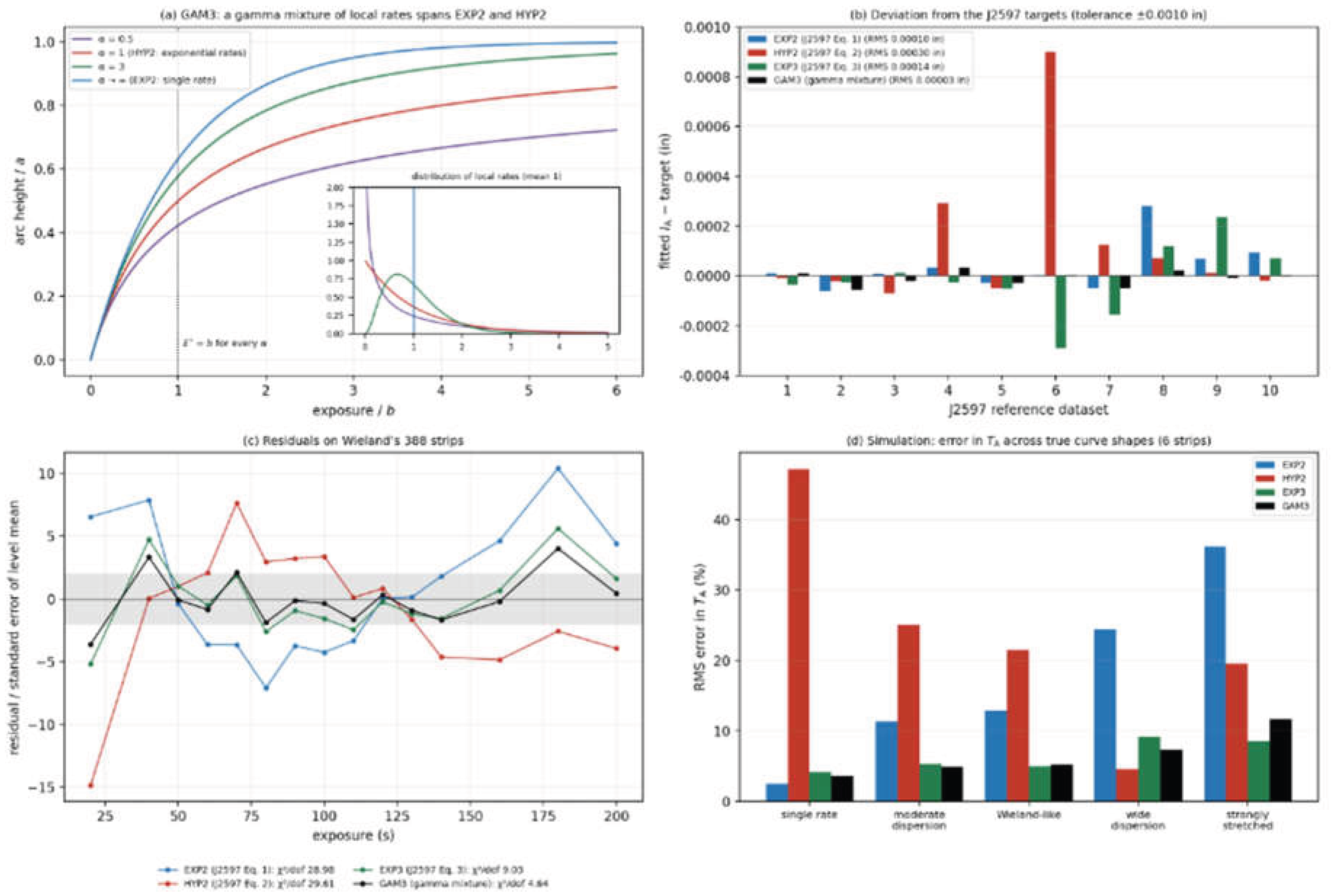
Properties. GAM3 has three properties that suit assurance. Its parameter is the inverse square of the coefficient of variation of the local rates, so it measures how uniform the peening of the strip is: large means a uniform, single-rate process, and falling over time signals growing dispersion from media wear, segregation or non-uniform exposure. Because it nests EXP2 and HYP2, a test of against its limits shows whether either simpler equation is adequate. And the exposure most sensitive to an exposure-rate set point, E*, is exactly its scale parameter for every , Equation (13), so that and its uncertainty are read directly from the fit. To our knowledge, this interpretation and its exposure properties do not appear in J2597, Kirk’s Solver Suite or the other saturation-curve literature we reviewed. The functional form itself is not new to Almen curves: Solís Romero et al. used h = A/b^p − A/(t + b)^p as a three-parameter regression for the saturation point [29], which is GAM3 with α = p, a = A/b^p and the GAM3 scale equal to b/p, without a mixture interpretation or the properties derived here.
Table 10.
Performance of GAM3 against the J2597 example equations and Kirk’s four-parameter form (Supplementary Data S5). Simulation: 400 replicates for each of five true curve shapes spanning single-rate to strongly stretched, strip standard deviation 0.00016 in.
Table 10.
Performance of GAM3 against the J2597 example equations and Kirk’s four-parameter form (Supplementary Data S5). Simulation: 400 replicates for each of five true curve shapes spanning single-rate to strongly stretched, strip standard deviation 0.00016 in.
| Equation | J2597 targets: RMS / max deviation (in) | Wieland: χ2 per degree of freedom | Wieland: cross-validated RMSE (in) | Wieland: IA/TA | Simulation: mean TA error, 6 / 4 strips | Simulation: IA RMSE, 6 strips (in) |
|---|---|---|---|---|---|---|
| EXP2 (J2597 Eq. 1) | 0.000100 / 0.000281 | 28.98 | 0.000215 | 12.56 / 63 s | 17.5% / 10.1% | 0.00017 |
| HYP2 (J2597 Eq. 2) | 0.000304 / 0.000900 | 29.61 | 0.000288 | 12.92 / 80 s | 23.6% / 13.1% | 0.00025 |
| EXP3 (J2597 Eq. 3) | 0.000138 / 0.000291 | 9.03 | 0.000223 | 12.66 / 68 s | 6.4% / 8.4% | 0.00014 |
| EXP3 + linear (Kirk) | 0.000119 / 0.000201 (3 sets) | 3.01 | 0.000137 | 12.58 / 66 s | not simulated | — |
| GAM3 (gamma mixture, Lomax form) | 0.000029 / 0.000056 | 4.64 | 0.000133 | 12.65 / 68 s | 6.6% / 7.1% | 0.00014 |
Re-run with Wieland’s data. The simulation above draws its true curves from rate-mixture families, which may favour rate-mixture equations. The simulation was therefore repeated with no assumed equation: the true curve is a monotone interpolation through Wieland’s fifteen level means ( in A, s), and each simulated strip carries the standard deviation Wieland measured at its exposure (0.00012–0.00021 in), for the designs used earlier and for one strip at each of Wieland’s fifteen levels (Table 11; 1000 replicates per cell).
What the re-run shows. With single strips at production scatter, the two-parameter exponential is at least as accurate as the three-parameter equations for intensity: on six strips its RMS intensity error is 0.00010 in against 0.16–0.17 for EXP3 and GAM3, and on the fifteen-level design 0.06 against 0.12–0.13, because its systematic misfit to Wieland’s curve, which dominates the of 388 averaged strips, is smaller than the scatter of a single strip. Characteristic exposure is recovered equally well by EXP2, EXP3 and GAM3 (RMS errors of 5–8%), and is recovered best by EXP2 and EXP3 (4–6%), whereas GAM3’s scale parameter is estimated less precisely (12–16%). With a clustered four-strip design (40–120 s) the three-parameter equations become unstable, with characteristic-exposure errors of 56–81% and occasional failed fits, while EXP2 stays at 10%. HYP2 is biased throughout, overestimating intensity by about 0.0004–0.0005 in and characteristic exposure by 23–41%, because Wieland’s curve is far less dispersed than its exponential distribution of rates assumes. These comparisons fit α afresh to each routine curve; Section 4.10 shows that fixing α at a value established in qualification removes the penalty.
Improvement over the J2597 equations. Against the J2597 targets, GAM3 reaches all ten within 0.00006 in, with an RMS deviation of 0.000029 in, against 0.100 for EXP2, 0.138 for EXP3 and 0.304 for HYP2: a three- to tenfold reduction, and a five- to sixteenfold reduction in the largest deviation. On Wieland’s 388 strips it reduces per degree of freedom from 29.0 (EXP2) and 29.6 (HYP2) to 4.6, half that of EXP3 (9.0), and lowers the cross-validated prediction error by 38–54% relative to the J2597 examples. In simulation across five plausible curve shapes it gives intensity errors of about 0.00014 in against 0.23–0.25 for the two-parameter forms, and characteristic-exposure errors of 6.6% (six strips) and 7.1% (four strips), against 17.5% and 10.1% for EXP2 and 23.6% and 13.1% for HYP2. The fitted for Wieland’s data is 3.1, a coefficient of variation of local rates of about 0.57; on the four-point reference sets runs to its upper bound, meaning EXP2 is adequate there, and on Sets 8–10 it falls to 0.5–1.3, the wide dispersion for which HYP2 also performs well.
Where the gain lies. The improvement is in characteristic exposure rather than intensity. All the saturating equations recover intensity within about 0.0001–0.00025 in, small against the in verification tolerance, and GAM3 and EXP3 agree on Wieland’s intensity to 0.000001 in. Characteristic exposure differs by up to 26% between the J2597 examples on the same data (63 s for EXP2, 68 s for EXP3 and GAM3, 80 s for HYP2). It carries coverage planning, exposure placement and the detection of flow faults. Therefore, it is where the choice of equation affects assurance.
Qualifications. Five qualifications apply. Kirk’s EXP3 with an added linear term fits Wieland’s data marginally better by (3.0) and has a similar cross-validated error (0.000137 in). However, it uses a fourth parameter, never saturates, gives a lower intensity (0.01258 in A) and has the largest prediction errors on the six-point reference sets. Among saturating equations GAM3 is the best supported. On the six-point reference sets the cross-validated errors of HYP2 and GAM3 are similar and smaller than those of EXP2 and EXP3. And the J2597 targets are consensus values that may themselves reflect several equations, so an equation spanning EXP2 and HYP2 is favoured by construction there. The stronger evidence is Wieland’s replicated data and the simulation. Two further qualifications concern the simulations. Where the true curve is drawn from rate-mixture families, the comparison tests recovery when the truth belongs to the GAM3 family, not discrimination between families. Where Wieland’s level means serve as truth, the comparison is a test of discrimination on one dataset, and it is not independent experimental evidence.
Recommendation. GAM3’s advantages are therefore of two kinds. Where information is plentiful, in qualification curves built from replicated strips at many exposures, misfit rather than scatter dominates and GAM3 describes the curve best among saturating equations, reproduces the J2597 targets most closely and supplies , a physically meaningful measure of rate dispersion. Where information is scarce, in routine curves of four to six single strips, a third free parameter costs more than it gains. The recommendation is accordingly: establish in a qualification curve with replicated strips; fit routine curves with GAM3 at the qualified , which keeps two fitted parameters as EXP2 does (Section 4.10); use EXP2 where qualification cannot reject a single rate; track as a dispersion diagnostic; and never fit a three-parameter equation to a clustered design. Because J2597 accepts any program that meets its Table 1, these choices are open to users of the Practice as it stands, although a solver at fixed must show that it meets Table 1 with declared.
Figure 5.
The gamma-mixture (Lomax) equation GAM3. (a) Curves and their distributions of local rates for , 1 (HYP2), 3 and ∞ (EXP2); = for every . (b) Deviation of fitted intensity from the J2597 targets for the three J2597 example equations and GAM3. (c) Residuals on Wieland’s 388 strips, scaled by the standard error of each level mean. (d) Error in characteristic exposure in simulation across five true curve shapes.
Figure 5.
The gamma-mixture (Lomax) equation GAM3. (a) Curves and their distributions of local rates for , 1 (HYP2), 3 and ∞ (EXP2); = for every . (b) Deviation of fitted intensity from the J2597 targets for the three J2597 example equations and GAM3. (c) Residuals on Wieland’s 388 strips, scaled by the standard error of each level mean. (d) Error in characteristic exposure in simulation across five true curve shapes.
4.9. The Saturation Curve as a Hardening Curve
Correspondence. The saturation curve has the shape of the monotonic stress–strain curve of an elastic–plastic metal, and the resemblance is structural. The J2597 example equations and Kirk’s four-parameter form are the standard work-hardening laws written in exposure: EXP2 is Voce’s saturation law [30], HYP2 the hyperbolic law of Kondner [31], EXP3 the stretched exponential of Hockett and Sherby [32], Kirk’s form a saturating law with added linear hardening, and GAM3 a continuous spectrum of saturating elements in the sense of Iwan’s distributed-element model [33]. In both cases a cumulative driver, plastic strain or exposure, builds an internal state that has a storage term and a saturation term. In a metal the state is the dislocation density, stored and dynamically recovered, which gives the Voce form [34]. In the strip it is the plastic layer, to which each impact adds until the layer reaches shakedown, after which further impacts on peened ground add little. Saturation is therefore shakedown of the impacted layer, a reading Al-Hassani anticipated when he named shakedown, reversed plastic yielding and the Bauschinger effect as part of the process [35]. A thermographic study of Almen samples found that the rate of rear-face heating fell by 17 to 27% when the strip reached saturation, as plastic dissipation would if the layer were shaking down, though not to zero [36]. For a single rate the governing equation is Equation (14), the analogue of Voce’s law. It is also the Avrami law of random coverage [37]: at , 10 = 2.303b and coverage is exactly 90%, the long-standing observation that saturation corresponds to about 90% coverage.
Meaning of the parameters. Read as a hardening curve, the parameters acquire mechanical meanings. The initial slope a/b plays the part of a modulus: before dents overlap it equals the arc-height contribution of one impact times the impact rate per unit area, which single-impact mechanics gives as the moment of one dent’s eigenstrain. The asymptote a plays the part of the saturation stress, set by the shakedown state and so by impact energy and the cyclic strength of the strip. The time scale b plays the part of the hardening strain constant, set by dent area and impact rate, and measures the spread of local rates as the spread of element strengths does in a distributed-element model. On Wieland’s 388 strips GAM3 gives a = 0.01443 in A, = 22.9 s and , so the initial slope is 0.00063 in/s, the local rates have a coefficient of variation of 0.57, = 2.98b, and the curve has reached 88% of its asymptote at (Supplementary Data S6). The analogy separates what the strip records into a single-impact term, a/b, and a shakedown term, a, which respond differently to faults, and gives the signatures of Section 4.10 a mechanical basis.
Reloading. A distributed-element model predicts reloading from the monotonic curve, as Masing’s rule does for cyclic loading [38], and GAM3 has an exact analogue. If peening is interrupted at t1 and resumed with each part of the strip receiving the same local rate, the fast elements are already saturated and the remaining rates are again gamma-distributed with the same shape and a lower mean. The continuation is GAM3 with replaced by + t1, Equation (15), which is simply the tail of the original curve. If the local rates are re-drawn on resumption, because the strip has been rotated or moved within the stream, the continuation restarts as a fresh GAM3 from h(t1), Equation (16), and saturates faster. For EXP2 the two coincide, because a single-rate process has no memory.
A test of what measures. This gives a direct test of what measures. Interrupting at and continuing to , Wieland’s parameters predict that a strip rotated or moved at the interruption reads 0.00052 in higher than one left in place if the dispersion is spatial, falling to 0.00037 in at 0.0015 and 0.00025 in at 2 ; against a single-strip standard deviation of 0.00016 in, five strips in each arm detect the difference at with ample power (Supplementary Data S6). If the dispersion arises within impact classes or through the depth of the layer rather than across the strip, moving the strip re-draws nothing and the two arms agree. With a single rate they agree in any case. The experiment therefore separates spatial non-uniformity of exposure, which a better fixture or nozzle path would remove, from dispersion intrinsic to the impact population, which only media control would change, a distinction that no single saturation curve can make. It also has a practical corollary: if the dispersion is spatial, a strip re-clamped in a different position after an interrupted run can read up to about 0.0005 in high near .
Limits. A saturation curve has no elastic limit; its departure from linearity comes from random overlap of impacts. Arc height integrates the eigenstrain moment through the strip, so the ‘material’ is the whole strip. And the analogy does not predict the asymptote, which needs impact mechanics and material transfer laws that lie outside this paper.
4.10. Generating and Verifying Saturation Curves
Principle. Existing practice fits EXP2, usually, to four or more strips around an expected saturation time, often a doubling series, and verifies with one strip at the established time within in. EXP2 is GAM3 with fixed at infinity, so every routine curve already assumes a value of ; the question is whether it is the right one. The proposed practice estimates once, in a qualification curve, and fixes it in every routine curve, which therefore keeps two fitted parameters, as EXP2 does, but carries the shape of the actual process.
Frozen reference. The qualification curve is approved once and frozen as h0(E), with its parameters, expected readings, uncertainties and chart limits. Verification compares strips with targets read from h0. It does not fit a second curve. A few verification strips cannot identify the parameters of a curve, and a fitted curve would absorb the drift that verification exists to detect. A routine curve may change h0 only through a controlled requalification, after the shape check, the measurement checks and an engineering review. The shape parameter α refitted from a routine curve is a diagnostic, not a replacement. Acceptance is unchanged. The strip at TA is judged as an absolute reading against the governing tolerance, and a chart alarm is an early warning that does not replace that decision.
Procedure. (1) Qualification: from one recorded strip lot, peen three strips at each of eight exposures log-spaced from 0.15 to 6 times the expected , under the production motion at a recorded position, and fit GAM3 with free; this fixes a, , , , and = , with uncertainties and a reference envelope. (2) Placement: take the expected from the previous curve or, for a new process, from a two-strip pilot. (3) Routine curve: six strips from one lot at 0.25, 0.43, 0.76, 1.3, 2.3 and 4.0 times the expected , each given one uninterrupted exposure or left in place if interrupted (Section 4.9), fitted with GAM3 at the qualified and reported with , and and their uncertainties. (4) Shape check: refit with free; an interval for that excludes the qualified value, or a lack-of-fit signal, requires requalification. Locally optimal designs cluster at the ends of the curve and cannot check the fit near , so the log-spaced design is preferred.
Against existing practice. The procedure was simulated on four curve shapes (Wieland’s, a stretched exponential, a single-rate and a widely dispersed process), with the strips placed for the right expected , one 30% short and one 40% long, and with estimated from a noisy qualification curve in every replicate (Supplementary Data S7; Figure 6(a)). Six strips at the qualified gave RMS errors of 4.0% in , 0.00011 in for and 8% in , against 10.5%, 0.00017 in and 39% for four strips with EXP2; the worst case fell from 25% to 5% in and from 0.00037 to 0.00014 in for . More strips do not rescue EXP2, whose misfit grows with the range spanned (16% on six strips), and four strips at the qualified (5.3%, 0.00013 in) also beat existing practice, so the gain comes from the equation. For a single-rate process the methods coincide. The main risk is a wrong qualified : in the widely dispersed case halving it biased by 0.00026 in and by 25%, and doubling it cost 13% in (Supplementary Data S7b), which is why the shape check is part of the procedure.
Figure 6.
Generating and verifying saturation curves (Supplementary Data S7). (a) RMS error in (plain bars) and (hatched) for existing practice (EP: EXP2 on four or six strips) and the proposed practice (PR: GAM3 with fixed at the qualified value), pooled over four curve shapes and three placements of the strips; triangles mark the worst case. (b) Change in arc height across the curve for six standard drifts of the Wieland process; dotted lines show of one strip and dashed lines the in tolerance. (c) Probability that one verification check detects a sustained loss of exposure rate (solid) or mass flow (dashed). (d) Detection probability in one check at the standard drifts; numbers give the mean number of checks to signal with EWMA charts. Single-strip verification within in detects none of the standard drifts in one check.
Figure 6.
Generating and verifying saturation curves (Supplementary Data S7). (a) RMS error in (plain bars) and (hatched) for existing practice (EP: EXP2 on four or six strips) and the proposed practice (PR: GAM3 with fixed at the qualified value), pooled over four curve shapes and three placements of the strips; triangles mark the worst case. (b) Change in arc height across the curve for six standard drifts of the Wieland process; dotted lines show of one strip and dashed lines the in tolerance. (c) Probability that one verification check detects a sustained loss of exposure rate (solid) or mass flow (dashed). (d) Detection probability in one check at the standard drifts; numbers give the mean number of checks to signal with EWMA charts. Single-strip verification within in detects none of the standard drifts in one check.
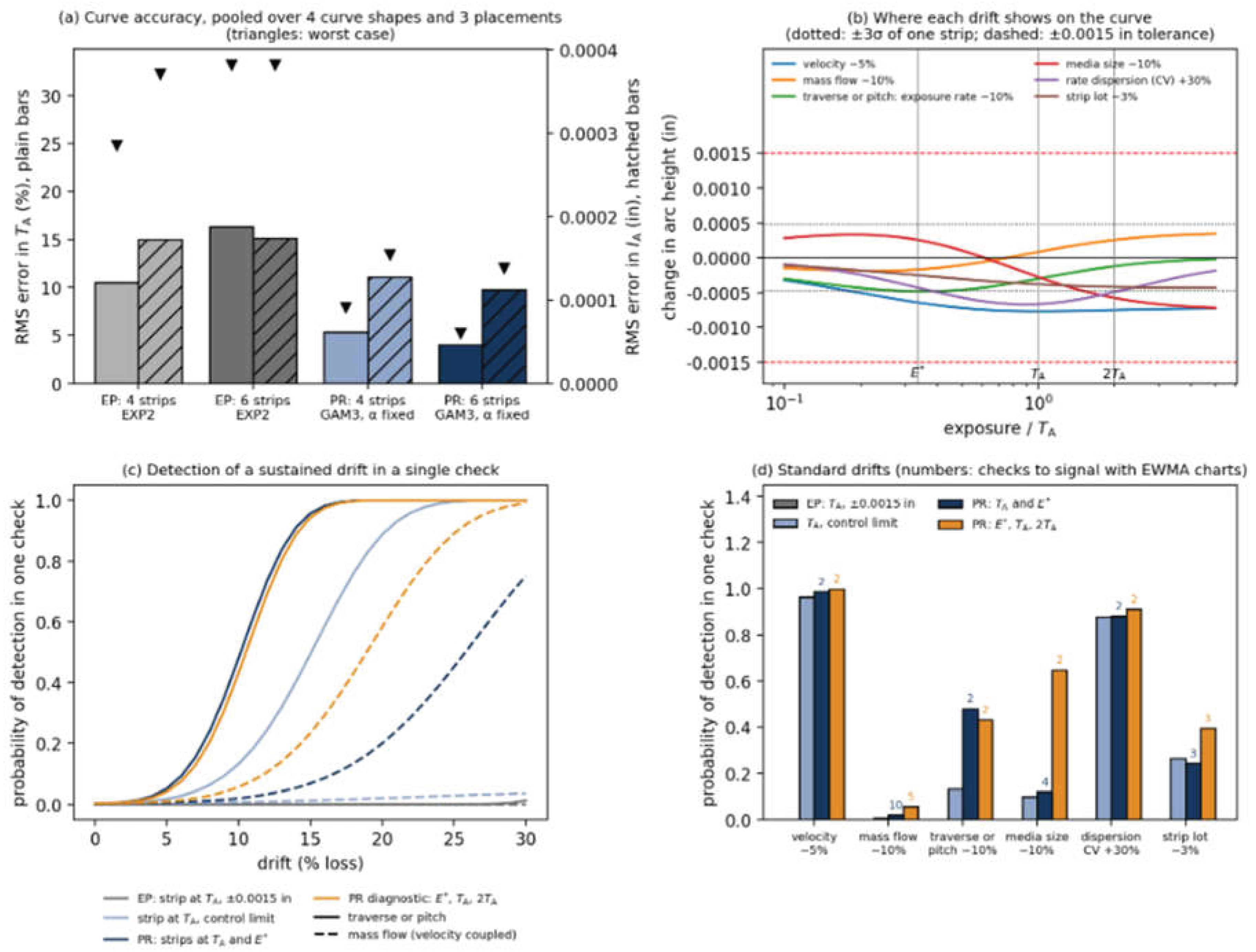
Sensitivity to process drift. Each drift moves a different part of the curve (Figure 6(b)). In the drift models of Supplementary Data S7, a 5% loss of velocity lowers the whole curve by 0.0006–0.0008 in; a 10% loss of exposure rate through traverse speed or raster pitch lowers it mainly near , by 0.00048 in, and hardly at all beyond ; a 10% loss of mass flow, which raises velocity through the loading effect of shot on the air stream, lowers it by 0.00017 in at but raises it by 0.00026 in at ; a 10% loss of media size raises it at and lowers it by 0.00058 in at ; a 30% rise in the dispersion of local rates lowers it most near , by 0.00067 in; and a 3% strip-lot shift scales it throughout. None of these moves a strip at outside in, so single-strip verification detects none of them in one check (Figure 6(c, d)): the tolerance is an acceptance limit, not a control limit. A routine curve at the qualified responds, moving by 5–15% against its scatter of 3%, so it flags the velocity and media-size drifts with certainty and the others with probability 0.56–0.76. Existing practice judges a new curve by intensity alone.
Where verification is most sensitive. A set-point change moves the curve, and a strip reads that change in proportion to the local sensitivity of the curve. For an exposure-rate set point (flow, traverse speed or pitch) the sensitivity is E dh/dE. For a velocity or pressure set point it is h + E dh/dE. Figure 7 plots both for the four equations fitted to Wieland’s strips. The most sensitive exposure E* for an exposure-rate set point depends on the equation. It is 0.43 TA for EXP2, 0.22 TA for HYP2, 0.38 TA for EXP3 and 0.34 TA for GAM3, where it equals the scale parameter b. A strip at TA keeps only 59 to 65% of the maximum sensitivity to an exposure-rate change. A strip at 2TA keeps 13 to 36%. For a velocity or pressure set point, EXP2, EXP3 and GAM3 peak at 0.87 to 0.99 TA, where verification already sits. HYP2 has no interior maximum.
Verification on the informative parts of the curve. Three exposures carry the information: , where exposure-rate faults are largest; , where velocity, dispersion and strip-lot faults are largest and where verification already sits; and , where media-size and mass-flow faults appear with the opposite sign to their effect at E*. Strips at and , charted against the qualified reference values with limits giving a combined false-alarm rate of 0.27% per check, detect a 10% loss of exposure rate in one check with probability 0.48, against 0.13 for a charted strip at alone and zero within the tolerance; with EWMA charts (, in-control run length 370) they signal every standard drift within about two to four checks except mass flow, which takes about ten. Adding a strip at raises single-check detection of media wear from 0.12 to 0.65 and halves the time to signal a mass-flow fault. It turns the three deviations into a signature: proportional changes at all three exposures indicate a strip-lot or intensity shift; a deficit at that has gone by indicates exposure rate; opposite signs at and separate mass flow (low, then high) from media size (high, then low); and a deficit largest at indicates growing dispersion.
A near-TA index that cancels strip lot. A strip at E* is the most powerful single reading of an exposure-rate fault, but E* lies well below TA, where acceptance is judged, and a strip-lot factor shifts every absolute reading. Two strips combined as a ratio avoid the second problem. With Y a measured reading and h0 the frozen reference curve, the index is;
V = ln[Y(EH) / Y(EL)] − ln[h0(EH) / h0(EL)]
V is zero under the approved baseline. A multiplicative factor common to both strips, such as a strip-lot or amplitude shift, cancels. A loss of exposure rate does not cancel, because it moves the two strips by different fractions. For the Wieland GAM3 fit the index is most sensitive to an exposure-rate change when the pair is centred on TA, at EL = 0.244 TA and EH = 0.976 TA. The rounded pair 0.25 TA and TA peaks at 0.976 TA. A 10% loss of exposure rate moves V by 0.044. With a strip scatter of 0.00016 in, that is 1.7 standard deviations in one check. Table 12 compares this with single strips.
The index is not more powerful than a strip at E*. Its advantage is that lot scale does not enter. With a 3% lot term, the standard deviation of one absolute strip rises from 0.00016 in to about 0.0003 in at E* and 0.0004 in at TA, and the one-check z falls to 1.6 and 0.7. The index stays at 1.7. It overtakes the strip at E* once the lot term reaches about 3% with one strip at each exposure, and about 1.4% with four, so it is worth using only where the lot term is not controlled by a lot-response factor (P12). The values assume independent strip scatter. They are not the detection probabilities of Figure 6, which include chart limits and a false-alarm rate. Limits for V must be fixed before any trial.
Reading IA and TA together. Machine settings move the curve (IA, TA) and some change its shape. A 10% rise in mass flow lowers IA by about 2% but TA by about 7%; a 5% rise in pressure raises IA by about 3% and lowers TA by about 3%; a 10% larger shot raises IA by about 5%. Supply-limited bore wear from 8.0 to 9.6 mm lowers IA by about 19% and lengthens TA by about 24%. Mass flow therefore moves mainly TA, which is why intensity-only records miss flow faults. TA is defined by a ratio (the 10% rule compares the arc height at 2T with that at T), so when all strips of a curve come from one lot, lot and thickness factors multiply every reading equally and cancel from TA, while IA carries them. Read together, a rise in velocity or pressure moves IA up and TA down, a loss of flow moves mainly TA, and a new strip lot moves IA alone. In simulated six-strip curves with Wieland's scatter, a 10% loss of mass flow shifts TA by 2.7 standard deviations, more than any single verification strip. A lot change does not move it (Supplementary Data S29).
Curve shape. Process geometry also changes the shape of the curve. Raster ripple barely affects it because the gauge averages the ripple. A stationary footprint smaller than the gauge span exposes the strip edges more slowly than the centre, delaying TA by 17 to 75% and widening the spread between equations to as much as 13%, so stationary and moving curves are not interchangeable. A wide impact-energy population stretches the curve, because large impacts keep adding depth after small ones saturate: the exponent of EXP3 falls to about 0.8, close to the 0.83 fitted to Wieland's data, and EXP2 fails the lack-of-fit check (Supplementary Data S30). Pressure fluctuation of ±2 to 5% gives about ±1 to 3% in IA, and mass-flow variation of ±5 to 10% gives about ±1 to 2% in IA but ±4 to 7% in TA, so TA is the less repeatable of the two. A published repeat of four four-point curves on one machine (1, 2, 4 and 8 revolutions) gave IA of 0.0112 to 0.0116 in A (CV 1.7%) and T1 of 2.65 to 3.68 revolutions (CV 15%, 95% interval 8 to 55%) [39], in line with the 0.00017 in and 10.5% predicted by simulation of four-strip EXP2 curves.
Proposed requirement. For any equation that passes the eligibility checks for a saturation curve, the curve report should state E* for an exposure-rate set point, the arc height h(E*) and the ratio of the sensitivities at TA and at E*. Where verification is meant to detect flow, traverse or pitch faults it should include a strip at E* as well as the strip at the qualified exposure, and TA should be recorded and trended with IA, each curve being built from one strip lot with six strips where practical. AMS2432E fixes its pressure and flow shutdown limits by two arc-height tests at the intensity time (3.7.2) [20]; at TA each carries only about 60% of the available flow sensitivity, so a strip at E* strengthens them. TA exists only for full curves, so where faster feedback is needed the strip at E* is the practical monitor.
When. At each verification interval set by the governing specification, peen the strip at , judged for acceptance against in as now, and a strip at , and chart both. Add the strip at after maintenance or media addition, at a declared routine interval, and whenever a chart signals, to classify the cause before any adjustment. Generate a new routine curve when a signal is not explained by a strip-lot check (Section 4.6) or when any frozen process variable changes, and requalify, with free, for a new process, nozzle type or media class, or when the shape check rejects the qualified . The extra cost is one strip per verification, one per diagnosis and two per routine curve. The drift models are first-order and assume Wieland’s strip scatter; Section 5.5 proposes a prospective test.
5. Discussion
5.1. Principal Interpretation
The strongest supported conclusion is conceptual and limited. Reproducing finite reference targets is evidence about a calculation method. An individual result also depends on measurement integrity, exposure support and modelling choices. The historical and simulated analyses show how these conditions can matter in specified examples. They neither validate the proposed gates nor establish field risk.
The framework changes the reporting question. It asks what evidence accompanied a number, not whether software returned one. A useful implementation would state the reporting equation, the exposure range, the number and direction of roots, the residual measure and the declared repeatability. It would also state the admissible comparison models, the tolerance ΔIA, and the consequence of each hold status.
5.2. Sensitivity to a Declared Comparison Family
EXP2, HYP2 and EXP3 do not span model-form uncertainty. External work should justify the comparison family in advance. It should add physically credible forms, alternative weighting, heteroscedastic error models and a shape-constrained nonparametric diagnostic. Kirk showed, with SAE data sets [8], that exposure range alone moves saturation heights by about 8% and saturation times by a factor of two. The definition being fitted has itself changed between revisions of J443 [40,41,42,43].
Position of the most sensitive exposure. The result that E* lies about one third of the way to TA is not an artefact of the gamma form. A lognormal and a bi-exponential mixture of local rates, fitted to Wieland’s data, place E* at 0.34 and 0.36 TA, against 0.34 for GAM3. The bi-exponential fits best, with an RMS error of 0.000049 in against 0.000072 in for GAM3 and 0.000079 in for the lognormal. It has four parameters, which a routine curve of six strips cannot identify.
5.3. Measurement Implications
Result 4 shows that a common additive offset can evade curve-shape checks. It does not identify the source of the offset. Pre-bow, mounting, gauge zero, thickness and hardness could have signed, multiplicative or interaction effects. A direct metrology study should measure the whole chain before any numerical lot-mean threshold or correction is proposed.
Strip lots add a practical implication (Section 4.6). A multiplicative lot effect moves IA without moving TA. Pre-bow and manufacturing residual stress move TA. The pair (TA, IA) therefore helps to diagnose the source when a result departs from its qualified value. A shift in intensity at constant characteristic exposure points to strip thickness or hardness. A shift in characteristic exposure points to pre-bow, strip residual stress or a change in the shot stream. Record the strip lot with every curve, build each curve from one lot, and verify each new lot against a reference lot before release.
5.4. Limitations
- The only replicated empirical dataset is a single 1993 experiment from one machine, strip lot, operator, gauge and laboratory. Bailey et al. compared old and new strip suppliers [13]. Mean arc heights differed by 0.004 in (as printed), and within-supplier standard deviations were 0.00016–0.00037 in. They noted that meeting the strip specification did not guarantee adequate intensity response. Section 4.6 shows that between-lot effects either set a floor on the uncertainty of intensity or, if lots are mixed, weaken the lack-of-fit test. Neither can be quantified from the Wieland data.
- The gauge and the strip carry further uncontrolled variation. J442 gives the dimensions of the Almen gauge but no calibration procedure. Flattened support balls can raise a 0.024 in A reading to almost 0.030 in A, about 25% [44]. Strips made by a hybrid route met all five J442 attributes (length, width, thickness, hardness and flatness). Yet they gave a bimodal distribution of arc heights at the same exposure, attributed to residual stress left by straightening [12]. Reported intensity also depends on the fitting rule. In one study two shot sizes gave 0.0063 in A and 0.0062 in A by the conventional definition, but 0.0065 in A and 0.0057 in A from an eight-point regression fit [45].
- Thresholds and challenge cases were developed and assessed on the same evidence; no locked independent test set exists.
- The canonical empirical benchmark uses PCHIP on the full-precision means. The linear-interpolation calculation and its resampling interval are sensitivity analyses and exclude grid, model, machine, operator and day-to-day uncertainty.
- The J2597 datasets have no replicates; Wieland’s repeatability was applied to them as an assumption.
- The million-curve analysis reduces Monte Carlo error under its data-generating model but does not increase the number of independent manufacturing systems.
- Exposure designs were sampled without a field-derived distribution, and no fault-prevalence model was used.
- Pre-bow scenarios assume a direct additive mechanism and a stipulated gauge error; those assumptions were not tested experimentally.
- The comparison family is narrow and the source materials did not include a shape-constrained nonparametric benchmark.
- The code, environment locks, per-curve outputs and a permanent repository identifier have not yet been deposited, and the numerical results have not been reproduced independently.
5.5. External Validation Programme
A defensible next study would lock the rule and implementation before testing. It would preregister thresholds and decision losses, and use independently authored cases and replicated multi-laboratory data. It should cross machines, shot streams, strip lots, operators, gauges, days and exposure designs, and add deliberately introduced measurement faults. It should report complete decision matrices by known truth condition, with the categories false eligibility, false hold, insufficient data, model inadequate, model sensitive and sensitivity not assessable. The study should also relate IA and TA errors to separately defined process-control and material-performance consequences.
A prospective comparison of the curve-generation and verification procedure of Section 4.10 with existing practice should accompany it. It should be run on one machine under deliberately introduced drifts. A second inexpensive experiment is the interrupted-exposure test of Section 4.9. It shows whether the dispersion of local rates is spatial or intrinsic to the impact population. The cheapest first step is a lot-response experiment. It extends the supplier’s annual sampling to the lots a user actually receives. Take 5–10 strips from each of several lots and suppliers. Peen them together at one reference condition and measure them on one calibrated gauge. The experiment would estimate the between-lot variance that the Wieland data cannot supply. It would test whether lots differ multiplicatively (intensity shifted, characteristic exposure unchanged) or additively. It would set the allowance in provision P12.
The comparison arms are single-strip verification at TA, charted strips at TA and E*, the log-ratio index V, and the full configuration of E*, TA and 2TA. The primary outcomes are one-check detection, average run length, false-alarm rate, robustness to strip-lot scaling, ability to distinguish fault types, added strip cost and time to disposition. Thresholds must be chosen before the blinded fault trials. The study should include pneumatic and wheel machines, because the machine-to-machine difference in the response of the strip to the stream is not known.
A shop can test the strip at E* directly. On a moving-nozzle setup, expose at least five strips from one lot at TA and at E* from the fitted curve (0.43 TA for EXP2), at the qualified traverse speed and with the speed changed by 10%. The reading at E* should shift 1.6 to 2 times as much as the reading at TA, which is 0.0004 to 0.0005 in against 0.00024 to 0.00032 in for a 10% change of exposure rate. The claim that a strip at E* adds sensitivity to exposure-rate faults is refuted if the ratio is below 1.2, or if the shift at E* lies within the strip scatter.
6. Conclusions
1. Matching the J2597 reference data does not make a result fit to report. All three J2597 example equations reach all ten targets, yet they differ in intensity by up to 0.0012 in on one dataset. A program can pass J2597 and still report a number that depends on the equation chosen.
2. Four checks decide whether a result is eligible for reporting: method, measurement, support and declared family. A result that fails any one is held. Under the declared rules nine of the ten reference datasets are eligible. Set 6 is held as model inadequate, a status that depends on a provisional threshold. The checks qualify one result. They do not qualify the process, and they do not show that a part will perform in fatigue.
3. Curve shape alone cannot prove a result. EXP2 and HYP2 force a single downward crossing whatever the data show, and finite points cannot identify a flexible curve. In simulation a common +0.0010 in lot offset passed every shape check and shifted reported intensity by 0.00091 to 0.00097 in. The checks must therefore cover the strips as well as the curve.
4. Strip-lot variation sets a floor that more strips cannot remove. A lot-to-lot coefficient of variation of 2–4% sets an equal floor on the relative uncertainty of intensity. Mixing lots can hide a poor equation: EXP3 stopped being rejected (p = 0.07) when two lots 2.5% apart were mixed. Build every curve from one recorded lot, and qualify each new lot against a reference lot.
5. The equation moves characteristic exposure far more than intensity. On Wieland’s data the saturating equations agree on intensity to within about 0.0001 to 0.00025 in. Characteristic exposure differs by up to 26% (63 s for EXP2, 68 s for EXP3 and GAM3, 80 s for HYP2). Exposure planning and fault detection depend on that quantity.
6. GAM3 is the better reporting equation once its shape is fixed from a qualification curve. GAM3, a gamma mixture of exponential rates, contains EXP2 and HYP2 as limits and reaches the J2597 targets three to ten times more closely than the example equations (RMS deviation 0.000029 in against 0.0001 to 0.0003 in). With its shape parameter fixed at the qualified value it cuts the error in characteristic exposure in simulation from about 10% to 4%, and the worst case from 25% to 5%. Fitted with the shape free to a few single strips it is no better than EXP2 for intensity. Never fit a three-parameter equation to a clustered exposure design.
7. Current practice leaves characteristic exposure uncertain by about 10%. The proposed procedure cuts that to about 4%. With four strips fitted with EXP2 and verification by one strip, the simulated RMS error is 10.5% in TA (24.8% in the worst case), 0.00017 in in intensity (0.00037 in worst case) and 39% in E*. Six strips fitted with GAM3 at the qualified shape give 4.0% (5.2%), 0.00011 in (0.00014 in) and 8%. That is 62 to 79% less error in TA and E* and 35 to 63% less in intensity. Verification by one strip within ±0.0015 in detects none of the six standard drifts in one check; charted strips at E* and TA detect a 10% loss of exposure rate with probability 0.48 and signal the standard drifts in 1.6 to 4.0 checks, mass flow in 9.6. The strip-lot floor of 2–4% is not reduced by the procedure; only lot control removes it. Table 13 gives the comparison.
8. A tolerance on one strip cannot detect process drift. A strip at TA within ±0.0015 in detected none of the six standard drifts in one check. Charted strips at E* and TA, with a strip at 2TA to classify the cause, signal every standard drift within about two to four checks. Mass flow is the exception, at about ten checks, or five with the strip at 2TA.
9. Freeze the qualification curve and verify against it. A curve fitted at verification absorbs the drift it is meant to detect. A two-strip log ratio at 0.25 TA and TA cancels strip-lot scale. It is less powerful than a strip at E* when the lot is controlled, and it wins once the lot term exceeds about 3% with one strip at each exposure, or 1.4% with four.
10. The saturation curve behaves as a work-hardening curve. The J2597 equations are the Voce, hyperbolic and Hockett–Sherby laws written in exposure, and saturation is shakedown of the impacted layer. This is an analogy of form, not a proved law. An interrupted-exposure test would show whether the dispersion of local rates is spatial.
11. The evidence is analytic, historical and simulated, so the next step is a prospective test. The results come from one machine, one replicated experiment and stated models. No threshold should be adopted until it has been locked and tested on independent data. The framework is ready to be tested, not yet ready to be adopted.
Author Contributions
[To be stated by the author.]
Funding
This research received no specific funding.
Data Availability Statement
Appendix D is the canonical transcription of Wieland’s historical readings and full-precision means; its two scan-resolved entries remain marked. The J2597 source observations remain subject to the source access terms. No external archive or DOI has been assigned yet. Supplementary Data S8 contains the full text of Section 5.2. Supplementary Data S7 and S7b contain the curve-generation, verification and drift simulations of Section 4.10 and Figure 6.
Code and reproducibility availability
A permanent, versioned archive should hold the raw and derived data, Appendix B fixtures, per-curve simulation outputs, seeds, package versions, optimiser settings, parameter bounds, failure rules, tolerances and one-command reproduction instructions. No archive has been deposited and no identifier assigned yet.
Use of Generative AI
Generative AI (Claude, Anthropic) was used to draft text, to retrieve and partition information from the cited sources, and to help design some of the numerical experiments. The author set the research questions and is responsible for the content.
Conflicts of Interest
[To be stated by the author.]
Appendix A. Research Specifications Requiring Validation
These provisions are research specifications requiring validation, neither validated nor normative. Bracketed quantities are provisional. Check any clause implication against a controlled copy before external use.
P1 Purpose of reference-data compliance. Compliance with the Table 5 reference datasets qualifies the calculation method under the declared fitting convention. It does not by itself make an individual Almen result eligible for reporting under the declared procedure. Each curve shall also be assessed against P2 to P6 and P9.
P2 Reporting equation. A four-point set shall use EXP2, a two-parameter equation, as the reporting equation; a six-point set shall use EXP3. The same rule applies to Table 5, Appendix B and the benchmark analyses. HYP2 is a comparison equation. Under EXP2, Sets 8 and 9 fail the provisional 3.5u adequacy limit; under the declared EXP3 rule they pass. The reporting equation shall leave at least two residual degrees of freedom and shall meet the prospectively locked performance criterion in P10. Clauses P3 to P5 apply to the reporting equation.
P3 Characteristic point. The program shall search for solutions of from the shortest to the longest measured exposure and shall report their number. An intensity shall be reported as ELIGIBLE FOR REPORTING UNDER THE DECLARED PROCEDURE only if there is exactly one solution and dR_A/d(ln E) at that solution is less than . Otherwise the status shall be NON SATURATION RESPONSE, except that the status shall be INSUFFICIENT DATA where the only solution lies beyond the longest measured exposure or is already below 0.10 at the shortest measured exposure.
P4 Measured support. An intensity shall be reported as ELIGIBLE FOR REPORTING UNDER THE DECLARED PROCEDURE only if at least one measured exposure is less than TA and at least one is equal to or greater than 2TA. Otherwise the status shall be INSUFFICIENT DATA.
P5 Fit adequacy. Where the fit has two or more residual degrees of freedom, the program shall report the largest residual as a multiple of the declared repeatability u. If it exceeds k(n_eff, α)·u, where n_eff is the number of independently assessed exposure means and α the target false-alarm rate, the status shall be MODEL INADEQUATE. The values of u and of k shall be established empirically from replicated measurements such that no more than [α = 5]% of curves from a stable process are flagged; the provisional value used in this article is k = 3.5. Tests of statistical significance shall not be used for this purpose. Where two or more strips are exposed at the same exposure, the test shall be applied to the exposure means, with the same limit, and if any two strips at the same exposure differ by more than [3]·√2·u the status shall be MODEL INADEQUATE. (The √2 follows from propagating two independent readings each of repeatability u; the multiplier is provisional and requires empirical calibration.) The repeatability u shall be established on strips whose pre-bow has been measured and subtracted with its sign.
P6 Model consequence. The program shall also fit each equation in the comparison family 𝓕 declared prospectively for the implementation. The admissible set is 𝓕_A = {reporting equation} ∪ {f ∈ 𝓕 : P3(f) ∧ P4(f) ∧ P5(f)}, and ΔI_A = max I_A,f − min I_A,f over f ∈ 𝓕_A. The program shall report |𝓕_A| and ΔI_A. If ΔI_A exceeds [δI_A], the status shall be MODEL SENSITIVE. If |𝓕_A| = 1, the status shall be MODEL SENSITIVITY: NOT ASSESSABLE; a single admissible equation is not evidence of insensitivity to equation choice. The comparison family does not restrict the choice of reporting equation.
P7 Reporting. The output shall state ELIGIBLE FOR REPORTING UNDER THE DECLARED PROCEDURE or NOT ELIGIBLE FOR REPORTING UNDER THE DECLARED PROCEDURE. A non-eligible output shall include at least one reason code: INSUFFICIENT DATA, NON SATURATION RESPONSE, MODEL INADEQUATE, MODEL SENSITIVE, MODEL SENSITIVITY: NOT ASSESSABLE or DATA INCONSISTENT. NOT ASSESSABLE does not permit reporting because the declared model-consequence check could not be completed. The output shall also state I_A, TA, the reporting equation, the number of P3 solutions, exposure range, |𝓕_A|, ΔI_A where defined, the TA range across the admissible family, ΔTA, and fit-based standard errors computed from both residuals and declared repeatability u. TA is indicative unless replicated doubling pairs bracket it. A non-eligible result shall not be reported as the peening intensity without disposition by the cognizant engineering authority.
P8 Challenge datasets. In addition to the Table 5 reference datasets, a program shall return the research-specification classification for each Appendix B fixture. Each fixture shall be published as point data and its intended classification confirmed by at least two independent implementations before adoption.
P9 Data consistency. If any measured arc height is lower than that at the preceding shorter exposure by more than [3]·√2·u, the result shall be NOT ELIGIBLE FOR REPORTING UNDER THE DECLARED PROCEDURE with reason code DATA INCONSISTENT. The multiplier shall be set with regard to the number of adjacent comparisons, since the chance of a false flag grows with the number of exposures.
P10 Prospective performance criterion. Once independently replicated benchmark datasets exist, the reporting equation, applied to curves built from single strips at the prescribed exposure designs, shall give intensity within ±[0.0005] in of the prospectively declared equation-independent benchmark in at least [95]% of eligible results, and TA within ±[10]% in at least [95]% of eligible results or report TA as indicative only. For the Wieland dataset, the declared benchmark is PCHIP on full-precision means: 65.85 s and 0.012589 in. Until independent benchmarks exist, P10 specifies needed evidence rather than an adoptable clause.
P11 Strip-lot identity. Every saturation curve shall be built from Almen strips of a single recorded manufacturing lot, and the lot identifier shall be reported with the result. A curve containing strips from more than one lot shall be reported as NOT ELIGIBLE FOR REPORTING UNDER THE DECLARED PROCEDURE unless the lots have been qualified as equivalent under P12.
P12 Lot-response qualification. Before release, a sample of strips from each new lot shall be peened at one declared reference condition together with strips from a retained reference lot. The lot shall be accepted if the difference in mean arc height lies within a declared allowance, and the observed between-lot variance shall be retained as an input to the uncertainty of reported intensity. The allowance and sample size remain to be established by the validation programme of Section 5.5.
P13 Set-point sensitivity. For the reporting equation, the curve report shall state the exposure E* at which a reading is most sensitive to an exposure-rate set point, the maximum of E·h′(E), together with h(E*) and the ratio of the sensitivity at TA to that at E* (Section 4.10). Where verification is intended to detect flow, traverse or pitch faults, it shall include a strip at E*.
P14 Exposure placement and transfer records. When machine settings, shot size or nozzle differ from those of an earlier eligible curve, the exposure series shall be planned from the expected TA, scaled from that curve, so that it spans TA to 2TA. Curves intended for comparison or transfer between machines shall record mean impact velocity at the strip position and mass loading.
P15 Reporting equation and curve generation. A qualification curve shall be generated for each process from one recorded strip lot, with three strips at each of eight exposures log-spaced over about 0.15–6 × the expected , and reported with GAM3 (Equation (12)), giving , , and with uncertainties. Routine curves shall use six strips at about 0.25, 0.43, 0.76, 1.3, 2.3 and 4.0 × the expected , fitted with GAM3 at the qualified , or with EXP2 where qualification cannot reject a single rate; shall be re-estimated from each routine curve and requalification triggered when its interval excludes the qualified value. Three-parameter equations shall not be fitted to clustered exposure designs, and a strip whose exposure is interrupted shall not be moved before it is resumed (Section 4.10). The qualification curve shall be frozen as the verification reference h0. Routine curves shall not update it, and any change shall follow controlled requalification.
P16 Trending of both results. J443 already requires T to be documented with every derived intensity (6.6); in addition, for every saturation curve, TA shall be trended with control limits alongside I_A, and a shift in either shall be attributed by its signature before process adjustment: velocity or pressure moves I_A and TA in opposite directions, mass flow moves mainly TA, and a change of strip lot moves only I_A (Section 4.10).
P17 Verification on the informative parts of the curve. Verification shall be separated into acceptance and fault detection. At each verification interval a strip at shall be judged against the acceptance tolerance and, with a strip at , charted against the qualified reference values with control limits, for example EWMA charts; a strip at shall be added after maintenance or media addition, at a declared routine interval and whenever a chart signals, and the cause attributed from the pattern of deviations at the three exposures before any process adjustment. A new routine curve shall be generated when a signal is not explained by a strip-lot check or when a frozen process variable changes; requalification is required for a new process, nozzle type or media class, or when the shape check rejects the qualified (Section 4.10). Where strip-lot scale is not controlled by P12, a log-ratio index V (Equation (17)) of strips at about 0.25 TA and TA may be charted in place of the strip at E*; its limits shall be fixed before use.
Appendix B. Internal Stress Test Fixtures
These author-constructed fixtures (Table B1) serve as versioned implementation tests. The labels are intended classifications, not externally established ground truth. Independent parties should add blinded cases without changing this set after a software version is locked.
Table B1.
Internal stress-test fixtures and their intended classifications.
| Case | Represents | Exposures | Arc heights (in) | Intended classification | Margin to limit |
|---|---|---|---|---|---|
| C1-R | Strip series stops short of 2TA | 2, 4, 6, 8 | 0.0044, 0.0061, 0.0067, 0.0070 | INSUFFICIENT DATA | 2TA is 1.20 × last exposure |
| C1-A | Matched accept case: As C1-R with last strip at 12 | 2, 4, 6, 12 | 0.0044, 0.0061, 0.0067, 0.0071 | MODEL SENSITIVITY: NOT ASSESSABLE | EXP2 2TA = 0.80 × last exposure; HYP2 2TA = 1.19 × last exposure; |𝓕_A| = 1 |
| C2-R | All strips before the 10% point | 1, 2, 3, 4 | 0.0027, 0.0044, 0.0055, 0.0061 | INSUFFICIENT DATA | 10% point at 1.22 × last exposure |
| C2-A | Matched accept case: Table 5 Set 1 | 4, 6, 8, 12 | 0.0060, 0.0069, 0.0070, 0.0070 | ELIGIBLE FOR REPORTING UNDER THE DECLARED PROCEDURE | Table 5 Set 1 |
| C3-R | One faulty strip mid-series | 0.25, 0.5, 0.75, 1, 2, 4 | 0.0108, 0.0129, 0.0137, 0.0144, 0.0147, 0.0164 | MODEL INADEQUATE | Largest residual 4.0u (limit 3.5u) |
| C3-A | Matched accept case: Table 5 Set 9 | 0.25, 0.5, 0.75, 1, 2, 4 | 0.0108, 0.0129, 0.0137, 0.0144, 0.0157, 0.0164 | ELIGIBLE FOR REPORTING UNDER THE DECLARED PROCEDURE | Table 5 Set 9; EXP3 largest residual 0.9u |
| C4-R | Falling shot stream at the end of the series | 0.25, 0.5, 0.75, 1, 2, 4 | 0.0081, 0.0096, 0.0100, 0.0103, 0.0106, 0.0096 | DATA INCONSISTENT | Fall of 0.0010 in (limit 0.00068 in) |
| C4-A | Matched accept case: Table 5 Set 8 | 0.25, 0.5, 0.75, 1, 2, 4 | 0.0081, 0.0096, 0.0100, 0.0103, 0.0108, 0.0113 | ELIGIBLE FOR REPORTING UNDER THE DECLARED PROCEDURE | Table 5 Set 8; EXP3 largest residual 1.2u |
| C5-R | No true knee (R ≡ 0.10) | 0.25, 0.5, 0.75, 1, 2, 4 | 0.0085, 0.0094, 0.0099, 0.0103, 0.0113, 0.0125 | NON SATURATION RESPONSE | EXP3 at declared bounds: a ≈ 0.147 in and b′ at 10⁻⁹; slope ratio −0.001 versus −0.05 limit; classification is bound-sensitive |
| C5-A | Matched accept case: Table 5 Set 8 | 0.25, 0.5, 0.75, 1, 2, 4 | 0.0081, 0.0096, 0.0100, 0.0103, 0.0108, 0.0113 | ELIGIBLE FOR REPORTING UNDER THE DECLARED PROCEDURE | Table 5 Set 8; EXP3 largest residual 1.2u |
| C6-R | No strip between TA and 2TA | 1.5, 2, 24, 32 | 0.0082, 0.0090, 0.0110, 0.0110 | MODEL SENSITIVE | ΔI_A 0.00071 in (limit 0.5) |
| C6-A | Matched accept case: Same curve with strips at 4, 6 and 8 in place of 24 | 1.5, 2, 4, 6, 8, 32 | 0.0082, 0.0090, 0.0103, 0.0108, 0.0109, 0.0110 | ELIGIBLE FOR REPORTING UNDER THE DECLARED PROCEDURE | ΔI_A 0.00031 in |
| C7-R | First strip already beyond TA | 3, 4, 6, 8 | 0.0064, 0.0067, 0.0069, 0.0069 | INSUFFICIENT DATA | TA is 0.89 × first exposure |
| C7-A | Matched accept case: Table 5 Set 7 | 2, 3, 4, 6 | 0.0055, 0.0066, 0.0067, 0.0068 | ELIGIBLE FOR REPORTING UNDER THE DECLARED PROCEDURE | Table 5 Set 7 |
Appendix C. Conditional Simulation Specifications and Detailed Figures
Table C1 records the synthetic random-search specification. Table C2 records the one-million-curve boundaries. These choices define the simulation population and therefore the estimand.
Table C1.
Synthetic random-search specification.
| Item | Specification |
|---|---|
| True curve types (equal probability) | (i) stretched exponential a[1 − exp(−(bt)^c)], a = 0.011 in, b ~ U(0.1, 1.0), c ~ U(0.4, 1.0); (ii) sum of two exponentials 0.011[w(1 − e−t/k1) + (1 − w)(1 − e−t/k2)], k1 ~ U(0.5, 3), k2 ~ U(5, 30), w ~ U(0.3, 0.8); (iii) hyperbolic 0.012 t/(b + t), b ~ U(1, 10) |
| Number of exposures | 49 or 6, equal probability |
| Exposure locations | Drawn without replacement from {0.5, 1, 1.5, 2, 3, 4, 6, 8, 12, 16, 24, 32} and sorted |
| Scatter | Independent N(0, 0.0001 in) added to each arc height; no rounding; negative values not excluded (none arose) |
| Fitting | Unweighted least squares. EXP3 bounds: a, b′, c ≥ 10⁻⁹ with no finite upper bounds; starts a_0 = max(y), b′_0 = 1/median(E), c_0 = 1; up to 200,000 evaluations |
| Root search | R_A(E) − 0.10 evaluated on a geometric grid of 20,000 points from E_min/20 to 50·E_max, roots refined by Brent’s method |
| Failed fits | None: all 1,500 attempted fits converged for both equations (1,500 attempted, 1,500 converged, 0 failed). Any failure would be classed as a non-release outcome |
| Classification | Accepted 10% crossing under both EXP2 and HYP2 (Q1, Q2); supported if Q3 holds for both; model-sensitive if |I_EXP2 − I_HYP2| > 0.0005 in |
| Trials and seed | 1,500 trials; NumPy default_rng(1); scripts not yet archived |
Table C2.
One-million-curve development simulation boundaries.
| Item | Boundary used | Basis |
|---|---|---|
| Strip readings | One of Wieland’s real readings at each exposure, drawn at random with replacement | Measured repeatability 0.00016 in [25] |
| Gauge resolution | Every reading rounded to 0.0001 in | Verified: J442_202602 (3.3.1) requires 0.001 mm (0.00005 in) resolution and 0.005 mm (0.0002 in) accuracy; 0.0001 in is the Nadcap minimum (AS7117A 5.1.2) |
| Strip flatness, J442 grade | Pre-bow magnitude from Wieland’s as-received batch, capped at 0.001 in | Verified: J442_202602 Table 1A, Grade 1 pre-bow ±0.025 mm (±0.001 in) for N and A strips |
| Strip flatness, Grade 1S | As above, capped at 0.0005 in | Verified: J442_202602 Table 1A, Grade 1S pre-bow ±0.013 mm (±0.0005 in); Grade 1S is mandatory under AMS2432E (3.2.2), which also forbids mechanically deforming strips to meet pre-bow |
| Orientation | Random sign per strip (uncorrected scenarios); consistent sign (lot-bias scenario) | Mounting practice not specified |
| Lot bias | Lot offset uniform within ±0.001 in, plus 0.00005 in per strip | Simulation boundary based on the Grade 1 pre-bow tolerance of J442_202602 Table 1A; J442 sets no explicit lot-to-lot limit |
| Signed correction | Pre-bow measured with a 0.00005 in reading error, rounded to 0.0001 in, subtracted with its sign | Section 4.5 |
| Number of exposures | Four to six | Simulation boundary; any standards clause requires controlled-copy review |
| Exposure values | Any four to six of Wieland’s fifteen exposures (20–200 s), no placement constraint | Simulation design assumption; see Section 2.6 |
| Tolerances shown | ±0.001 in (J2597), ±0.0015 in (AMS2430U 3.11.2 verification), ±0.0005 in (δI_A, illustrative), 0.004 in band (illustrative) | J2597_201709 [1], J442_202602 [24] and J443_202512 [20] clause values verified against controlled copies |
| Checks | Candidate research specification: u = 0.00016 in, k = 3.5, δI_A = 0.0005 in, εS = 0.05, P9 limit 0.00068 in | Provisional values |
| Fitting | Separable least squares: exact over the amplitude, numerical over the remaining parameters; agrees with standard nonlinear least squares within 0.3% on the J2597 datasets, with equal or lower residual sum of squares | — |
| Not modelled | Holder flatness (0.001 in [24]), day-to-day, machine, operator and gauge-to-gauge variation | Would add to the errors shown |
| Curves and seeds | 200,000 per strip condition, 1,000,000 in total, run in batches of 2,000–20,000 with fixed seeds; per-curve results stored so alternative rules can be evaluated on the same curves; scripts not yet archived | — |
| Alternative rules tested | Graded support (last exposure ≥ 1.75TA, 1.5TA or 1.25TA) and planned series (spanning TA,emp to 2TA,emp) | Section 4.4 |
Figure C1.
Detailed one-million-curve results. Every percentage is a conditional frequency under resampling from Wieland’s single-system historical data and the specified exposure, fitting, and error model. The figure does not estimate field prevalence or external operating performance. Within the graphic, ‘released’ means ‘eligible for reporting under the declared procedure.’
Figure C1.
Detailed one-million-curve results. Every percentage is a conditional frequency under resampling from Wieland’s single-system historical data and the specified exposure, fitting, and error model. The figure does not estimate field prevalence or external operating performance. Within the graphic, ‘released’ means ‘eligible for reporting under the declared procedure.’
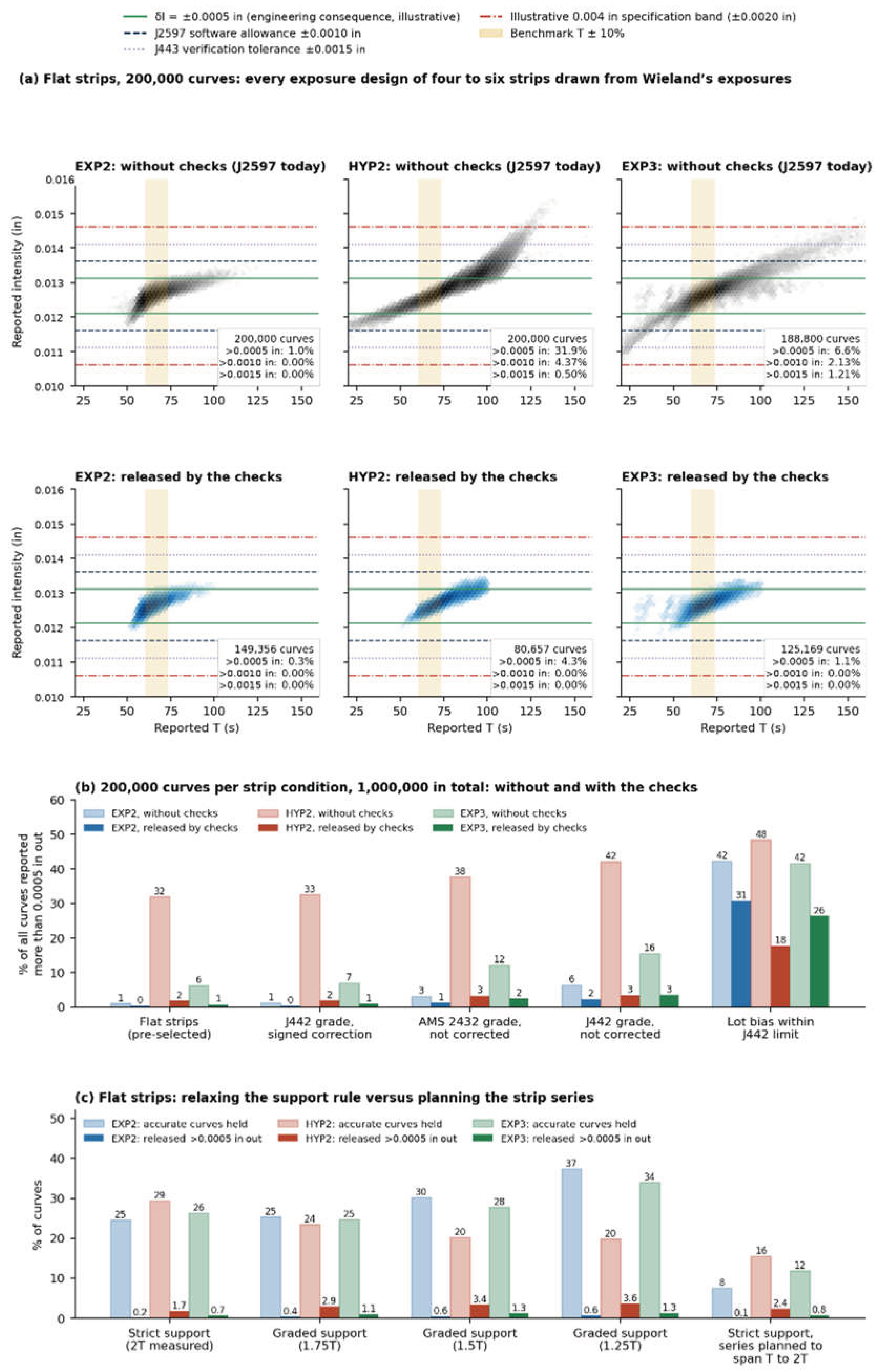
Figure C2.
Conditional pre-bow scenario results for 250 curves per scenario. Bars describe the stipulated additive and correction models; they do not establish production prevalence, actual orientation practice, or a justified lot-mean limit. Within the graphic, ‘released’ means ‘eligible for reporting under the declared procedure.’
Figure C2.
Conditional pre-bow scenario results for 250 curves per scenario. Bars describe the stipulated additive and correction models; they do not establish production prevalence, actual orientation practice, or a justified lot-mean limit. Within the graphic, ‘released’ means ‘eligible for reporting under the declared procedure.’
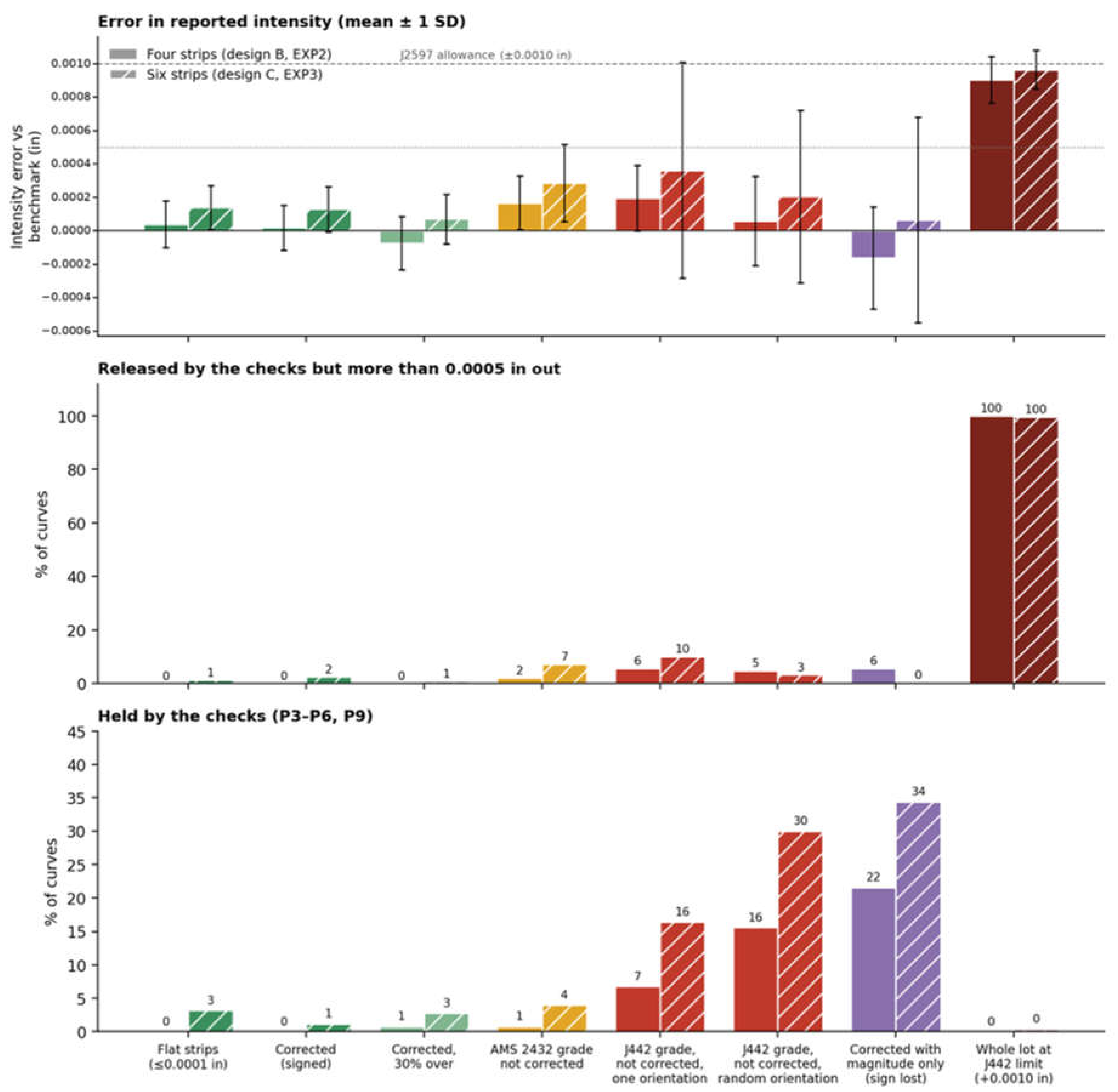
Figure C3.
Flexible-function construction behind Result 3. The constructed curve agrees at every checked point while changing crossing topology between observations. The alternative is intentionally unrestricted and is not asserted to be a common physical response. Legacy graphic labels t/T correspond to E/TA.
Figure C3.
Flexible-function construction behind Result 3. The constructed curve agrees at every checked point while changing crossing topology between observations. The alternative is intentionally unrestricted and is not asserted to be a common physical response. Legacy graphic labels t/T correspond to E/TA.
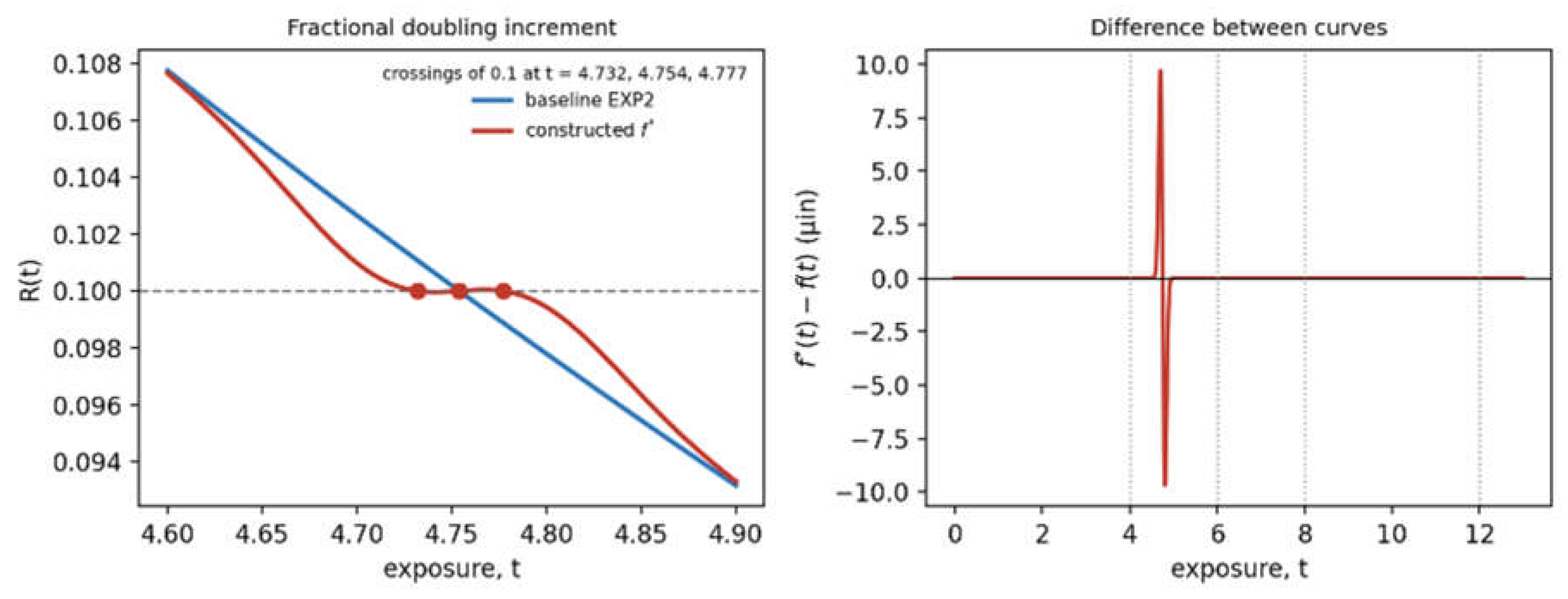
Appendix D. Canonical Wieland Dataset
Table D1 is the canonical Wieland dataset. Columns are exposure times in seconds. Arc heights are in thousandths of an inch, as printed by Wieland (multiply by 0.001 to obtain inches), and the Mean row retains the full-precision values used for the PCHIP benchmark. The dagger marks two entries resolved from printed column statistics because the scan was illegible; the value was identified at column level but its row remains uncertain.
Table D1.
Canonical Wieland dataset: arc height (thousandths of an inch, as printed) for each strip at each exposure, with sample size, mean and standard deviation.
Table D1.
Canonical Wieland dataset: arc height (thousandths of an inch, as printed) for each strip at each exposure, with sample size, mean and standard deviation.
| # | 20 s | 40 s | 50 s | 60 s | 70 s | 80 s | 90 s | 100 s | 110 s | 120 s | 130 s | 140 s | 160 s | 180 s | 200 s |
|---|---|---|---|---|---|---|---|---|---|---|---|---|---|---|---|
| 1 | 7.6 | 10.9 | 11.7 | 12.5 | 12.7 | 13.0 | 13.3 | 13.5 | 13.4 | 14.0 | 13.7 | 13.9 | 14.3 | 14.1 | 14.4 |
| 2 | 7.3 | 11.1 | 11.9 | 12.5 | 12.9 | 12.9 | 13.4 | 13.4 | 13.8 | 13.9 | 13.5 | 13.9 | 14.0 | 14.2 | 14.5 |
| 3 | 7.4 | 10.5 | 11.8 | 12.2 | 12.6 | 13.0 | 13.4 | 13.4 | 13.3 | 13.6 | 13.8 | 13.9 | 14.2 | 14.7 | 14.0 |
| 4 | 7.8 | 11.0 | 11.9 | 12.3 | 12.6 | 12.9 | 13.1 | 13.7 | 13.8 | 13.6 | 13.9 | 13.9 | 14.4 | 14.3 | 14.1 |
| 5 | 7.7 | 11.0 | 11.4 | 12.3 | 12.8 | 12.9 | 13.1 | 13.5 | 13.5 | 13.9 | 13.7 | 14.0 | 14.0 | 14.2 | 14.0 |
| 6 | 7.4 | 11.1 | 11.7 | 12.6† | 12.6 | 13.0 | 13.1 | 13.5 | 13.5† | 13.8 | 13.8 | 13.9 | 13.9 | 14.1 | 14.1 |
| 7 | 7.7 | 10.9 | 11.6 | 12.4 | 13.0 | 12.9 | 13.2 | 13.5 | 13.6 | 13.8 | 14.0 | 13.9 | 14.1 | 14.5 | 14.6 |
| 8 | 7.7 | 10.8 | 11.7 | 12.2 | 12.7 | 12.9 | 13.2 | 13.5 | 13.5 | 13.8 | 13.9 | 14.1 | 13.9 | 14.2 | 14.2 |
| 9 | 7.6 | 10.7 | 11.4 | 12.6 | 12.8 | 13.2 | 13.2 | 13.2 | 13.6 | 13.5 | 13.8 | 13.8 | 14.0 | 14.4 | 14.3 |
| 10 | 7.4 | 11.0 | 11.6 | 12.0 | 13.0 | 13.2 | 13.3 | 13.3 | 13.6 | 13.5 | 13.8 | 13.8 | 14.2 | 14.2 | 14.2 |
| 11 | 11.0 | 11.7 | 12.0 | 12.8 | 13.1 | 13.5 | 13.6 | 13.9 | 13.9 | 13.8 | 13.9 | 13.9 | 14.2 | ||
| 12 | 11.1 | 11.6 | 12.0 | 12.6 | 12.9 | 13.4 | 13.3 | 13.6 | 13.8 | 13.5 | 14.0 | 14.1 | 14.3 | ||
| 13 | 10.8 | 11.8 | 12.6 | 12.8 | 12.9 | 13.5 | 13.6 | 13.6 | 13.3 | 14.0 | 13.7 | 14.0 | 14.4 | ||
| 14 | 11.0 | 11.9 | 12.3 | 12.9 | 13.0 | 12.8 | 13.7 | 13.6 | 13.9 | 14.0 | 13.9 | 14.1 | 14.3 | ||
| 15 | 11.0 | 11.6 | 12.1 | 12.8 | 13.0 | 13.1 | 13.4 | 13.3 | 13.7 | 13.8 | 13.6 | 14.0 | 14.2 | ||
| 16 | 11.0 | 11.8 | 12.3 | 12.8 | 13.0 | 13.3 | 13.4 | 13.9 | 13.8 | 14.0 | 14.0 | 14.2 | 14.3 | ||
| 17 | 10.9 | 11.7 | 12.4 | 12.7 | 13.0 | 13.2 | 13.3 | 13.8 | 13.8 | 14.0 | 14.0 | 14.1 | 14.2 | ||
| 18 | 10.9 | 11.8 | 12.2 | 12.6 | 13.4 | 13.1 | 13.7 | 13.9 | 14.0 | 13.6 | 14.0 | 13.9 | 14.4 | ||
| 19 | 10.9 | 11.6 | 12.1 | 12.7 | 12.9 | 13.6 | 13.6 | 13.5 | 13.7 | 13.8 | 14.0 | 14.0 | 14.4 | ||
| 20 | 11.1 | 11.3 | 12.3 | 12.9 | 13.0 | 13.6 | 13.5 | 13.6 | 13.8 | 13.8 | 13.8 | 13.9 | 14.1 | ||
| 21 | 10.8 | 11.7 | 12.1 | 12.8 | 12.9 | 13.6 | 13.3 | 13.6 | 13.9 | 13.9 | 14.0 | ||||
| 22 | 11.1 | 11.4 | 12.3 | 12.5 | 13.3 | 13.5 | 13.4 | 13.8 | 13.9 | 14.2 | 13.9 | ||||
| 23 | 11.0 | 11.7 | 12.2 | 12.8 | 12.8 | 13.4 | 13.6 | 13.3 | 13.8 | 13.5 | 14.0 | ||||
| 24 | 10.8 | 11.7 | 12.1 | 12.9 | 12.9 | 13.4 | 13.6 | 13.5 | 13.5 | 13.9 | 13.9 | ||||
| 25 | 10.5 | 11.8 | 11.9 | 12.9 | 12.9 | 13.3 | 13.6 | 13.6 | 13.6 | 14.0 | 14.0 | ||||
| 26 | 11.1 | 11.8 | 12.1 | 12.9 | 13.0 | 13.4 | 13.5 | 13.5 | 14.1 | 14.0 | 13.8 | ||||
| 27 | 11.1 | 11.6 | 12.2 | 12.7 | 12.8 | 13.3 | 13.4 | 13.6 | 13.8 | 14.1 | 13.7 | ||||
| 28 | 11.0 | 11.9 | 12.5 | 12.8 | 13.2 | 13.0 | 13.6 | 13.5 | 13.9 | 13.9 | 14.2 | ||||
| 29 | 11.6 | 12.2 | 12.7 | 12.9 | 13.2 | 13.5 | 13.5 | 13.8 | 13.6 | 13.8 | |||||
| 30 | 11.6 | 12.1 | 12.9 | 13.2 | 13.4 | 13.5 | 13.7 | 14.0 | 13.8 | 14.0 | |||||
| n | 10 | 28 | 30 | 30 | 30 | 30 | 30 | 30 | 30 | 30 | 30 | 30 | 20 | 20 | 10 |
| Mean | 7.560 | 10.932 | 11.677 | 12.253 | 12.773 | 13.000 | 13.297 | 13.487 | 13.597 | 13.780 | 13.837 | 13.910 | 14.060 | 14.285 | 14.240 |
| SD | 0.171 | 0.166 | 0.157 | 0.193 | 0.128 | 0.146 | 0.190 | 0.131 | 0.169 | 0.179 | 0.177 | 0.124 | 0.143 | 0.150 | 0.207 |
Appendix E. Fitting Settings
These settings are part of the fitting convention (Section 2.3). They must be locked before external evaluation.
EXP3 parameters a, b′ and c are bounded below by 10−9, with no finite upper bound. The starting values are a0 = max(y), b′0 = 1/median(E) and c0 = 1. At most 200,000 function evaluations are allowed.
The root function RA(E) − 0.10 is evaluated on a 20,000-point geometric grid from Emin/20 to 50Emax. Roots are refined by Brent’s method. A failed fit is a non-release outcome.
References
- SAE International. SAE J2597_201709, Computer generated shot peening saturation curves; SAE International: Warrendale, PA, 2017. [Google Scholar] [CrossRef]
- Kirk, D. Satisfactory peening intensity curves. Shot Peen. 2012, 26(4), 24–32. [Google Scholar]
- Kirk, D. Estimating peening intensity. Shot Peen. 2024, 38(4), 26–32. [Google Scholar] [CrossRef]
- Huyton, P. Mandatory application of SAE J2597 computer generated shot peening saturation curves. Metal. Finish. News 2018, 19. Available online: https://mfn.li/archive/issue_view/1828/1.
- Kirk, D. Saturation curve analysis and quality control. Shot Peen. 2006, 20(3), 24–30. [Google Scholar]
- Kirk, D. Saturation Curve Solver Suite user’s instruction manual, IM:0097, Release 09; Electronics Inc: Mishawaka, IN, 2009. [Google Scholar]
- Electronics Inc. (2017). PeenSolver web application, www.peensolver.com. Introduced in Barkley, D. (2017). PeenSolver: your free curve solver web app. The Shot Peener, 31(2), 22. Library document 2017016.
- Kirk, D. Accuracy of computerized saturation curve analysis. Shot Peen. 2006, 20(1), Library document 2006005. [Google Scholar]
- Kirk, D. J443: an evolutionary guide to shot peening intensity measurement. Shot Peen. Library document 2012015. 2012, 26(2), 24–32. [Google Scholar]
- Kirk, D. Accuracy of declared peening intensity values. Shot Peen. 2010, 24(2), Library document 2010011. [Google Scholar]
- Kirk, D. Metrology of Almen arc height measurement. Shot Peen. 2008, 22(2), Library document 2008009. [Google Scholar]
- Champaigne, J.M. Performance of Almen strips which are straightened after hardening. In Proceedings of the 8th International Conference on Shot Peening (ICSP-8), Garmisch-Partenkirchen, 2002. [Google Scholar]
- Bailey, P.G.; Lombardo, D.R.; Popp, H.G.; Thompson, R.A. Full assurance shot peening of aircraft gas turbine engine components. In Proceedings of the 6th International Conference on Shot Peening (ICSP-6), San Francisco, 1996; pp. 320–327. [Google Scholar]
- Draper, N.R.; Smith, H. Applied Regression Analysis, 3rd ed.; Wiley: New York, 1998. [Google Scholar]
- Automotive Industry Action Group. Measurement Systems Analysis Reference Manual, 4th ed.; AIAG: Southfield, MI, 2010. [Google Scholar]
- Joint Committee for Guides in Metrology. JCGM 100:2008, Evaluation of measurement data – Guide to the expression of uncertainty in measurement; BIPM: Sèvres, 2008. [Google Scholar] [CrossRef]
- Kennedy, M.C.; O’Hagan, A. Bayesian calibration of computer models. J. R. Stat. Soc. Ser. B 2001, 63(3), 425–464. [Google Scholar] [CrossRef]
- SAE International. SAE J442_202602, Tools for peening intensity determination and verification. 2026. [Google Scholar] [CrossRef] [PubMed]
- SAE International. SAE J443_202512, Procedures for determining and verifying peening intensity. 2025. [Google Scholar] [CrossRef]
- SAE International. AMS2432E, Shot peening, computer monitored; SAE International: Warrendale, PA, 2022. [Google Scholar] [CrossRef]
- SAE International. SAE J2277_202301, Shot peening coverage determination. 2023. [Google Scholar] [CrossRef]
- SAE International. AMS2430U, Shot peening; 2018. [Google Scholar] [CrossRef]
- SAE International. AMS2431E, Peening media, general requirements; 2023. [Google Scholar] [CrossRef]
- Wieland, R.C. A statistical analysis of the shot peening intensity measurement. In Proceedings of the 5th International Conference on Shot Peening, Oxford, 1993; pp. 27–38. [Google Scholar]
- Efron, B.; Tibshirani, R.J. An Introduction to the Bootstrap; Chapman and Hall: New York, 1993. [Google Scholar]
- Lomax, K.S. Business failures: another example of the analysis of failure data. J. Am. Stat. Assoc. 1954, 49(268), 847–852. [Google Scholar] [CrossRef]
- Johnson, N.L.; Kotz, S.; Balakrishnan, N. Continuous Univariate Distributions, 2nd ed.; Wiley: New York, 1994; vol. 1. [Google Scholar]
- Vaupel, J.W.; Manton, K.G.; Stallard, E. The impact of heterogeneity in individual frailty on the dynamics of mortality. Demography 1979, 16(3), 439–454. [Google Scholar] [CrossRef]
- Solís Romero, J.; de los Rios, E.R.; Levers, A.; Karuppanan, S. Towards the optimisation of the shot peening process in terms of fatigue resistance of the 2024-T351 and 7150-T651 aluminium alloys. WIT Trans. Eng. Sci. 2001, 33. [Google Scholar] [CrossRef]
- Voce, E. The relationship between stress and strain for homogeneous deformation. J. Inst. Met. 1948, 74, 537–562. [Google Scholar]
- Kondner, R.L. Hyperbolic stress–strain response: cohesive soils. J. Soil Mech. Found. Div. ASCE 1963, 89(SM1), 115–143. [Google Scholar] [CrossRef]
- Hockett, J.E.; Sherby, O.D. Large strain deformation of polycrystalline metals at low homologous temperatures. J. Mech. Phys. Solids 1975, 23(2), 87–98. [Google Scholar] [CrossRef]
- Iwan, W.D. A distributed-element model for hysteresis and its steady-state dynamic response. J. Appl. Mech. 1966, 33(4), 893–900. [Google Scholar] [CrossRef]
- Kocks, U.F.; Mecking, H. Physics and phenomenology of strain hardening: the FCC case. Prog. Mater. Sci. 2003, 48(3), 171–273. [Google Scholar] [CrossRef]
- Al-Hassani, S.T.S. An engineering approach to shot peening mechanics. In Proceedings of the 2nd International Conference on Shot Peening (ICSP-2), Chicago, 1984; pp. 275–282. [Google Scholar]
- Pron, H.; Henry, J.-F.; Flan, B.; Lu, J.; Offermann, S.; Beaudoin, J.L. Estimation of residual stresses induced by shot-peening: measurement of the thermal dissipation with an infrared camera. Int. J. Therm. Sci. 2002, 41, 369–375. [Google Scholar] [CrossRef]
- Avrami, M. Kinetics of phase change. I. General. Theory J. Chem. Phys. 1939, 7(12), 1103–1112. [Google Scholar] [CrossRef]
- Masing, G. Eigenspannungen und Verfestigung beim Messing. In Proceedings of the 2nd International Congress of Applied Mechanics, Zürich, 1926; pp. 332–335. [Google Scholar]
- Waelchli, E. How time affects Almen strip arc height: a two-year research program explores the validity of archiving Almen strips. Shot Peen. 2022, 36(1), 20–21. [Google Scholar]
- Kirk, D. Peening intensity: true meaning and measurement strategy. Shot Peen. 2016, 30(3), Library document 2016030. [Google Scholar]
- Kirk, D. The Solver story: an autobiography. Shot Peen. 2019, 33(2). [Google Scholar]
- Kirk, D. Back to basics: peening intensity. Shot Peen. 2021, 35(2), 26–30. [Google Scholar]
- Kirk, D. Two strip setting-up and verification program for peening intensity. Shot Peen. 2010, 24(4). [Google Scholar]
- Champaigne, J.M. Almen gage calibration. In Proceedings of the 8th International Conference on Shot Peening (ICSP-8), Garmisch-Partenkirchen, 2002; pp. 108–113. [Google Scholar]
- Tufft, M.K. (1996). Development of a fracture mechanics methodology to assess the competing mechanisms of beneficial residual stress and detrimental plastic strain due to shot peening. Paper presented at the 6th International Conference on Shot Peening (ICSP-6), San Francisco. Library document 1996125.
Figure 7.
Where verification is most sensitive. (a) EXP2, HYP2, EXP3 and GAM3 fitted to Wieland’s 388 strips as in Table 10, with TA (triangles) and the exposure E* most sensitive to an exposure-rate set point (open circles). (b) Sensitivity of the reading to an exposure-rate set point, E dh/dE, against exposure relative to the TA of each equation; E* is the peak. (c) Sensitivity to a velocity or pressure set point, h + E dh/dE; HYP2 has no interior maximum. (d) Share of the maximum exposure-rate sensitivity kept by a strip at TA (plain) and at 2TA (hatched).
Figure 7.
Where verification is most sensitive. (a) EXP2, HYP2, EXP3 and GAM3 fitted to Wieland’s 388 strips as in Table 10, with TA (triangles) and the exposure E* most sensitive to an exposure-rate set point (open circles). (b) Sensitivity of the reading to an exposure-rate set point, E dh/dE, against exposure relative to the TA of each equation; E* is the peak. (c) Sensitivity to a velocity or pressure set point, h + E dh/dE; HYP2 has no interior maximum. (d) Share of the maximum exposure-rate sensitivity kept by a strip at TA (plain) and at 2TA (hatched).
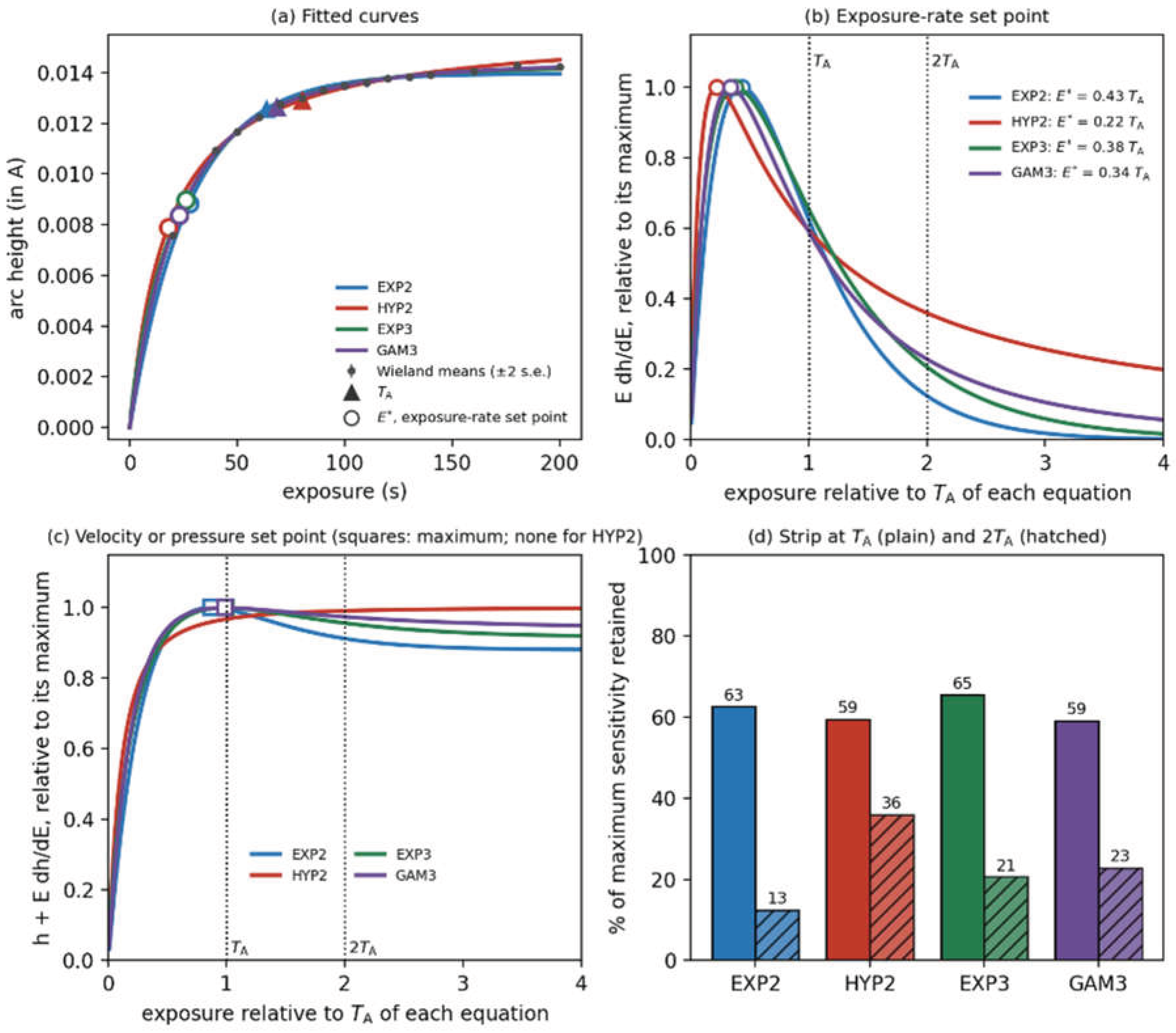
Table 1.
Notation.
| Symbol or term | Meaning |
|---|---|
| Exposure coordinate for a declared response curve. | |
| Measured or fitted Almen arc-height response at exposure | |
| Earliest supported Almen characteristic exposure satisfying | |
| Reported Almen intensity from the declared reporting equation. | |
| Almen fractional doubling increment | |
| Local exposure-amplification factor : the vertical-to-horizontal geometric sensitivity of Result 2, not a condition number. | |
| a, c | Curve-fit parameters only: asymptotic amplitude, exposure-scale parameter and EXP3 shape exponent. |
| Scalar amplitude of the flexible perturbation in Result 3 only. | |
| Standard uncertainty or declared single-strip repeatability. |
Table 2.
Conceptual framework.
| Condition | Question | Evidence reported | Decision meaning |
|---|---|---|---|
| Method | The implementation reproduces reference results under a verified controlled-copy procedure | Named reference datasets, equation and numerical settings | Calculation method qualified or not qualified |
| Measurement | Strip readings and corrections are traceable and internally consistent | Repeatability basis, signed corrections, lot and gauge records | Supported or measurement evidence incomplete |
| Support | Measured exposures bracket the region used to infer the characteristic point | Exposure range relative to fitted and | Supported or insufficient data |
| Declared family | The reporting equation fits adequately and the result is not materially sensitive within a declared comparison set | Residual criterion, admissible models, and model list | Eligible for reporting under the declared procedure, model inadequate, model sensitive, or sensitivity not assessable |
Table 3.
Data sources and what each supplies.
| Source | What it supplies | Use in this paper |
|---|---|---|
| SAE J2597_201709 | Ten reference datasets (seven with four observations, three with six; Sets 8–10 in inverse feed rate) and consensus targets [1,2]. A program must reach all ten targets within ±0.001 in and comply with J443. | Fits of EXP2, HYP2 and EXP3; tests of the reporting rule (Section 4.1) |
| SAE J443_202512 | Intensity from a saturation curve of at least four strips other than zero, fitted to J2597 where possible; intensity is the arc height that rises 10% when exposure doubles, with T documented (4.2, 4.3.5, 4.3.6.1, 6.6); one verification strip within ±0.0015 in, at most 8 h apart (4.5.1, 4.5.2); verification range may be narrowed asymmetrically (6.5). | Definition of intensity; verification tolerance used throughout |
| AMS2430U | Curve at each verification location per J443; verification strip within ±0.0015 in of the process-sheet arc height; intensity within −0/+30% of the specified minimum or 0.003 in; verification at the start and end of each lot or every eight machine hours (3.8.1.1, 3.11, 4.2.1.1). | Tolerance and interval in the worked examples |
| AMS-S-13165A (cancelled) | Support rule: at least four points, one at no less than double the saturation time; saturation is where doubling exposure raises arc height by no more than 10% (4.2.3). | Origin of the exposure-support check |
| Other standards checked | J2277_202301, J444_202306, AMS2431/1G, /2G, /3F, /4E, /6D and /8D, the superseded AMS2432B, J2441. | Clause checks only |
| Wieland experiment [24] | 388 strips from one lot, one air-blast system, one operator and one gauge, at 15 exposures from 20 to 200 s. Appendix D reproduces the printed sample counts and full-precision means; two entries resolved from scans are marked. | Benchmark, fits, resampling, lot and lack-of-fit tests |
Table 4.
Scope of the four analytical results.
| Result | Assumptions | What is established | What is not established | Empirical evidence still needed |
|---|---|---|---|---|
| 1 | EXP2 or HYP2 with positive parameters | The 10% crossing is unique and downward by model form | That the measured physical response saturated or has that topology | Replicated observations or an independently justified physical response class |
| 2 | Vertical perturbation evaluated locally along a fitted EXP2 or HYP2 curve | Local vertical-to-horizontal geometric sensitivity is 3.9 or 5.5 | A condition number or sampling variance for the fitted estimator | Design- and covariance-based uncertainty analysis under realistic error structures |
| 3 | Finite observations and an unrestricted sufficiently flexible alternative | Point agreement cannot identify the topology between observations | That physically plausible Almen curves commonly contain extra knees | A prospectively defined, physically constrained function class and targeted experiments |
| 4 | A positive additive offset common to all arc heights | The offset lowers and moves the 10% point earlier | That production pre-bow creates a constant offset, or how prevalent it is | Controlled signed pre-bow experiments across lots, orientations, gauges and sites |
Table 8.
Sensitivity of fitted intensity to deleting or perturbing one observation of the ten J2597 datasets.
Table 8.
Sensitivity of fitted intensity to deleting or perturbing one observation of the ten J2597 datasets.
| Measure | EXP2 | HYP2 |
|---|---|---|
| Datasets within ±0.0010 in after every single-observation deletion | 10 of 10 | 9 of 10 (Set 6 fails) |
| Worst case after one deletion | Within the allowance | Set 6: deleting the longest exposure moves intensity 0.00199 in, to 0.00289 in above target |
| Largest change in intensity from perturbing one reading by ±0.0001 in | 0.00007 in | 0.00012 in |
| Largest change in intensity from perturbing one reading by ±0.0005 in | 0.00036 in | 0.00064 in |
| Most influential observation | Longest exposure (all datasets) | Longest exposure (all datasets) |
Table 9.
Changes in characteristic exposure and intensity relative to the single-lot fits (EXP2 63.2 s, 0.012555 in A; HYP2 81.2 s, 0.012949 in A; EXP3 68.3 s, 0.012659 in A).
Table 9.
Changes in characteristic exposure and intensity relative to the single-lot fits (EXP2 63.2 s, 0.012555 in A; HYP2 81.2 s, 0.012949 in A; EXP3 68.3 s, 0.012659 in A).
| Lot scenario | EXP2: ΔTA (s), ΔIA | HYP2: ΔTA (s), ΔIA | EXP3: ΔTA (s), ΔIA |
|---|---|---|---|
| All readings × 0.95 | 0.0, −5.0% | 0.0, −5.0% | 0.0, −5.0% |
| All readings × 1.05 | 0.0, +5.0% | 0.0, +5.0% | 0.0, +5.0% |
| +0.0010 in offset, uncorrected | −3.4, +6.9% | −7.6, +5.9% | −3.0, +6.9% |
| −0.0010 in offset, uncorrected | +3.9, −6.8% | +9.3, −5.9% | +3.0, −6.9% |
| Lot step: for ≤ 90 s, for ≥ 100 s | +11.0, +2.9% | +24.4, +5.4% | +22.3, +5.1% |
Table 11.
Monte Carlo with a model-free truth through Wieland’s level means and Wieland’s level-specific strip standard deviations (Supplementary Data S5).
Table 11.
Monte Carlo with a model-free truth through Wieland’s level means and Wieland’s level-specific strip standard deviations (Supplementary Data S5).
| Design | Equation | IA bias / RMSE (in) | TA bias / RMSE | E* RMSE | Fits failing |
|---|---|---|---|---|---|
| typical 4-strip (40, 60, 80, 120 s) | EXP2 | -0.00019 / 0.00024 | -9% / 10% | 8% | 0.0% |
| HYP2 | +0.00041 / 0.00050 | +23% / 26% | 36% | 0.0% | |
| EXP3 | +0.00034 / 0.00078 | +23% / 56% | 39% | 4.9% | |
| GAM3 | +0.00047 / 0.00099 | +36% / 81% | 32% | 6.4% | |
| optimised 4-strip (20, 40, 160, 180 s) | EXP2 | +0.00017 / 0.00019 | -7% / 7% | 5% | 0.0% |
| HYP2 | +0.00046 / 0.00048 | +41% / 41% | 27% | 0.0% | |
| EXP3 | +0.00018 / 0.00020 | -2% / 7% | 5% | 0.0% | |
| GAM3 | +0.00016 / 0.00019 | -0% / 7% | 12% | 0.0% | |
| 6-strip (20, 40, 60, 90, 140, 200 s) | EXP2 | -0.00000 / 0.00010 | -7% / 7% | 6% | 0.0% |
| HYP2 | +0.00051 / 0.00053 | +37% / 38% | 29% | 0.0% | |
| EXP3 | +0.00010 / 0.00017 | +3% / 7% | 5% | 0.0% | |
| GAM3 | +0.00009 / 0.00016 | +4% / 8% | 15% | 0.0% | |
| EXP3+linear | -0.00008 / 0.00020 | -3% / 8% | 13% | 1.2% | |
| Wieland 15-level design, one strip per level | EXP2 | -0.00001 / 0.00006 | -5% / 5% | 4% | 0.0% |
| HYP2 | +0.00044 / 0.00045 | +31% / 31% | 32% | 0.0% | |
| EXP3 | +0.00010 / 0.00013 | +5% / 6% | 5% | 0.0% | |
| GAM3 | +0.00009 / 0.00012 | +5% / 7% | 16% | 0.0% | |
| EXP3+linear | -0.00001 / 0.00010 | -0% / 5% | 12% | 0.1% |
Table 12.
One-check detection of a 10% loss of exposure rate, as the signal divided by its standard deviation, for the Wieland GAM3 curve and a strip scatter of 0.00016 in. Lot variation is a multiplicative factor common to the strips of a lot. The values are development calculations, not detection probabilities.
Table 12.
One-check detection of a 10% loss of exposure rate, as the signal divided by its standard deviation, for the Wieland GAM3 curve and a strip scatter of 0.00016 in. Lot variation is a multiplicative factor common to the strips of a lot. The values are development calculations, not detection probabilities.
| Configuration | Strips | Use | One-check z, no lot variation | One-check z, 3% lot variation |
|---|---|---|---|---|
| Minimum acceptance | TA | Compliance with the governing tolerance | 1.9 | 0.7 |
| Power first | E* and TA | Rate-fault detection plus acceptance (value for the strip at E*) | 3.0 | 1.6 |
| Near-TA index | 0.25 TA and TA | Amplitude-invariant diagnostic centred on TA | 1.7 | 1.7 |
| Full diagnostic | E*, TA and 2TA | Classifies rate, mass-flow, media-size and dispersion signatures | as power first | as power first |
Table 13.
Uncertainty under current practice and under the proposed procedure (simulation of the Wieland process, strip scatter 0.00016 in; current practice: four strips fitted with EXP2 and one verification strip within ±0.0015 in; proposed: six strips fitted with GAM3 at the qualified shape and charted strips at E* and TA).
Table 13.
Uncertainty under current practice and under the proposed procedure (simulation of the Wieland process, strip scatter 0.00016 in; current practice: four strips fitted with EXP2 and one verification strip within ±0.0015 in; proposed: six strips fitted with GAM3 at the qualified shape and charted strips at E* and TA).
| Quantity | Current practice | Proposed procedure | Improvement |
|---|---|---|---|
| RMS error in characteristic exposure | 10.5% | 4.0% | 62% smaller |
| Worst-case RMS error in characteristic exposure | 24.8% | 5.2% | 79% smaller |
| RMS error in intensity | 0.00017 in | 0.00011 in | 35% smaller |
| Worst-case RMS error in intensity | 0.00037 in | 0.00014 in | 63% smaller |
| RMS error in E*, the most sensitive exposure | 39% | 8% | 79% smaller |
| RMS deviation from the ten J2597 targets | 0.00010 to 0.00030 in (EXP2, EXP3, HYP2) | 0.000029 in (GAM3) | 3 to 10 times smaller |
| Probability that one check detects a 10% loss of exposure rate | 0 (single strip within ±0.0015 in) | 0.48 (charted strips at E* and TA) | from none to about one in two |
| Checks needed to signal the six standard drifts | None signalled | 1.6 to 4.0; mass flow 9.6 (5.1 with a strip at 2TA) | all six signalled |
| Strip-lot floor on the uncertainty of intensity | 2–4% | 2–4% (unchanged) | none from the curve procedure; needs single-lot curves and lot qualification |
Disclaimer/Publisher’s Note: The statements, opinions and data contained in all publications are solely those of the individual author(s) and contributor(s) and not of MDPI and/or the editor(s). MDPI and/or the editor(s) disclaim responsibility for any injury to people or property resulting from any ideas, methods, instructions or products referred to in the content. |
© 2026 by the authors. Licensee MDPI, Basel, Switzerland. This article is an open access article distributed under the terms and conditions of the Creative Commons Attribution (CC BY) license (http://creativecommons.org/licenses/by/4.0/).
Copyright: This open access article is published under a Creative Commons CC BY 4.0 license, which permit the free download, distribution, and reuse, provided that the author and preprint are cited in any reuse.