

Submitted:
07 October 2026
Posted:
09 October 2026
You are already at the latest version
Abstract
Vehicle-to-Everything (V2X) networks may experience intermittent connectivity and frequent link disruption due to high node mobility, variable density, and heterogeneous mobility patterns. When a contemporaneous end-to-end path cannot be guaranteed, Delay-Tolerant Networking (DTN) enables message delivery through store-carry-forward communication. Among DTN routing protocols, PRoPHET exploits historical and transitive encounters to estimate destination-specific delivery predictability. However, its conventional Greater Than (GRTR) forwarding rule has limited contextual awareness because relay selection is based primarily on relative delivery predictability. This paper proposes ProphetRouterRL, a two-stage routing protocol that augments PRoPHET with Q-learning. First, PRoPHET identifies eligible relay candidates satisfying ΔP > 0. A Q-learning agent then determines whether to send or hold each message using a six-dimensional state comprising relay-buffer availability, encounter history, message load, remaining time-to-live, hop count, and node type. ProphetRouterRL was evaluated against conventional PRoPHET using the ONE Simulator in a map-based urban scenario representing the UKM Bangi area in Malaysia. The seven-day simulation comprised 129 heterogeneous nodes, including pedestrians, cyclists, cars, buses, metro trains, and stationary communication points. ProphetRouterRL increased the delivery probability from 46.47% to 93.12%, while reducing routing overhead and average latency by 39.4% and 41.4%, respectively. These results demonstrate the potential of combining PRoPHET’s delivery-predictability estimation with context-aware learned forwarding decisions in opportunistic V2X environments.
Keywords:
delay tolerant networks
; V2X communication
; reinforcement learning
; Q-Learning
; PRoPHET routing
; opportunistic networks
; vehicular networks
1. Introduction
Vehicle-to-Everything (V2X) communication is an important component of intelligent transportation systems, enabling information exchange between vehicles, roadside infrastructure, pedestrians, and communication networks through Vehicle-to-Vehicle (V2V), Vehicle-to-Infrastructure (V2I), Vehicle-to-Pedestrian (V2P), and Vehicle-to-Network (V2N) communication [1]. V2X services are primarily supported by two technology families: IEEE 802.11p-based Dedicated Short-Range Communications (DSRC) and Cellular-V2X (C-V2X), including LTE-V2X and 5G New Radio V2X (NR-V2X) [2]. These technologies enable applications such as collision warning, traffic coordination, and cooperative perception [3,4].
However, conventional V2X communication does not always provide a contemporaneous end-to-end path, particularly under sparse traffic, limited roadside-infrastructure coverage, urban obstruction, or network disruption. Vehicular Delay-Tolerant Networking (VDTN) addresses such conditions through store-carry-forward communication [5]. A node stores a message when no suitable forwarding path is available, carries it while moving, and forwards it when an appropriate relay or destination is encountered [6,7]. Thus, vehicle mobility can create future forwarding opportunities rather than being treated solely as a cause of link disruption. Because delivery may be delayed, this approach is primarily suitable for delay-tolerant V2X applications rather than latency-critical safety services [4].
Urban V2X environments contain vehicles, pedestrians, cyclists, public transport, and fixed roadside infrastructure with heterogeneous mobility, connectivity, and contact patterns. Together with variable vehicle density, wireless obstruction, and limited infrastructure coverage, these characteristics can produce rapidly changing or intermittently connected network topologies. Conventional routing protocols that require a contemporaneous end-to-end path may therefore perform poorly under such conditions, motivating VDTN routing protocols that select forwarding opportunities over time. Among DTN routing protocols considered for opportunistic V2X scenarios, the Probabilistic Routing Protocol using History of Encounters and Transitivity (PRoPHET) estimates destination-specific delivery predictability from direct encounters, aging, and transitive contact information [8,9]. Compared with Epidemic routing, which extensively replicates messages among encountered nodes [10], PRoPHET uses delivery predictability to identify relays with stronger historical delivery potential. This selective approach can reduce unnecessary replication and resource consumption, although its performance depends on mobility, traffic load, buffer capacity, and contact conditions.
However, the conventional PRoPHET forwarding strategy relies primarily on the relative delivery predictability of the current carrier and the encountered node. Although this metric captures historical and transitive contact information, the forwarding decision does not jointly consider message urgency and current relay-resource conditions [11]. Consequently, a relay may exhibit higher delivery predictability while being unsuitable under the current message and network state.
Reinforcement learning (RL) provides a means of introducing adaptive, context-aware decision-making into this process. In particular, Q-learning is a model-free RL algorithm that can estimate the long-term utility of alternative actions from accumulated experience without requiring an explicit analytical model of vehicle mobility or contact dynamics [12]. Previous studies indicate that RL-assisted routing can improve trade-offs among message delivery, routing overhead, delay, and resource utilization in opportunistic vehicular networks [11]. Nevertheless, existing approaches have largely employedly treated RL as a standalone routing mechanism rather than combining learned forwarding decisions with PRoPHET’s delivery-predictability estimation [11,13].
Accordingly, this study investigates a hybrid approach in which PRoPHET identifies forwarding opportunities based on historical delivery potential, while Q-learning determines whether an eligible opportunity should be accepted or deferred according to the broader message and relay state. The objective is to improve the balance among message delivery, routing overhead, and end-to-end latency without replacing PRoPHET’s established predictability mechanism.
The remainder of this paper is organized as follows. Section 2 reviews related work on DTN routing in opportunistic V2X environments and reinforcement-learning-based routing, before identifying the research gap and presenting the contributions of this study. Section 3 describes the system model, including the network environment, PRoPHET formulation, and performance metrics. Section 4 presents ProphetRouterRL, including its two-stage architecture, state representation, reward function, and Q-learning algorithm. Section 5 describes the simulation setup and evaluation methodology, while Section 6 presents and analyzes the results. Section 7 discusses the principal findings, implications, and limitations. Finally, Section 8 concludes the paper and outlines directions for future research.
2. Related Work
This section surveys vehicular routing studies that are applicable to intermittently connected V2X environments, representative DTN routing strategies, and learning-based approaches to improve opportunistic forwarding. The review specifically addresses the limitations of conventional PRoPHET which justify the introduction of the ProphetRouterRL framework.
2.1. DTN Routing in Vehicular Networks
DTN routing uses store-carry-forward communication to deliver messages across a sequence of opportunistic contacts when an end-to-end path does not continuously exist [6,7]. Representative approaches include Epidemic routing, Spray and Wait, and PRoPHET, which differ mainly in the way they control replication and select relay nodes.
Epidemic routing copies messages to encountered nodes which do not have them already, potentially achieving high delivery under favourable resource conditions but producing significant transmission and storage overhead [10]. Spray and Wait restricts this replication by giving each message a finite copy budget. Message copies are distributed during the spray phase, after which their carriers wait for direct contact with the destination [14]. Although this limits resource consumption, its fixed copy budget does not explicitly evaluate the delivery suitability of individual relays.
PRoPHET takes a more selective approach by exploiting the non-randomness of node encounters. It estimates destination-specific delivery predictabilities from direct encounters, aging, and transitive contact information [8]. Unlike Epidemic routing, PRoPHET uses these estimates to preferentially forward messages through nodes with stronger historical delivery potential, thereby limiting indiscriminate replication. Nevertheless, the default Greater Than (GRTR) relay-selection rule relies primarily on the relative delivery predictability of the current carrier and the encountered node [9]. Although delivery predictability represents historical and transitive contact information, the GRTR comparison does not jointly incorporate message urgency, current relay-resource conditions, or node heterogeneity. Previous studies suggest that such contextual information can improve forwarding decisions in dynamic vehicular and opportunistic networks [11,15,16]. This limitation has motivated extensions that supplement probabilistic routing with contextual information or adaptive decision-making.
2.2. Reinforcement Learning for DTN Routing
Opportunistic DTN forwarding can be formulated as a sequential decision-making problem because the effect of a forwarding action may only become evident after several subsequent encounters. A relay selected at one encounter may improve the probability of eventual delivery, but it may also consume transmission and buffer resources without contributing to delivery. Reinforcement learning (RL) is suitable for this setting because it can learn forwarding policies from interactions with the network environment while accounting for delayed outcomes [12]. Under an RL formulation, the observable message and network conditions constitute the state, forwarding alternatives constitute the actions, and delivery performance and resource consumption inform the reward. Q-learning as a model free RL is particularly relevant because it learns state–action values without requiring an explicit transition model of node mobility and future contacts [12,17]. However, its effectiveness depends strongly on the state representation, action definition, and reward design.
Several recent studies have applied reinforcement learning and related online-learning methods to routing in intermittently connected networks. Rezaei and Derakhshanfard [11] integrated Q-learning with PRoPHET-derived routing information. Their formulation uses an encounter-based state and a multi-copy action space, allowing RL to influence the delivery and replication decision. This differs from the present work, which retains PRoPHET’s GRTR comparison as an eligibility gate and applies Q-learning only to the subsequent binary send–hold decision.
Phutela et al. [18] proposed LearnRouter, an adaptive routing protocol based on the multi-armed bandit framework. LearnRouter employs the Upper Confidence Bound algorithm to balance exploration of alternative forwarding choices against exploitation of previously successful choices. It reported improved delivery and delay relative to several conventional and learning-based baselines. Unlike ProphetRouterRL, however, LearnRouter operates as an independent routing mechanism and does not retain PRoPHET’s delivery-predictability comparison as a separate relay-eligibility stage.
Schindlegger and Hupperich [13] proposed Spray-Learn-Wait, which combines movement-based node clustering with Q-learning within a spray-based routing architecture. The protocol reported improvements in delivery and overhead relative to PRoPHET, although with increased latency in the evaluated scenarios. It therefore represents an RL-assisted extension of the Spray-and-Wait lineage rather than an augmentation of PRoPHET.
Table 1 summarized further distinction between the three recent studies. Collectively, they use learning to modify PRoPHET-derived routing criteria, construct independent adaptive routing mechanisms, or enhance spray-based forwarding. However, they do not examine the explicit functional separation adopted in this work: PRoPHET’s conventional GRTR comparison first determines relay eligibility, after which Q-learning evaluates whether the eligible opportunity should result in a send or hold action. This separation preserves PRoPHET’s encounter-based delivery estimation while allowing additional message and relay context to influence the final forwarding decision.
2.3. Positioning, and Contributions
This functional separation also guides the state-space design. Because the sign of has already been used to determine relay eligibility, it is excluded from the RL state to maintain a compact Q-table. The learning stage instead considers contextual variables not jointly evaluated by the conventional GRTR comparison, including message urgency, forwarding history, relay-resource conditions, and node type.
Furthermore, existing RL-based DTN studies are commonly evaluated in generic opportunistic-network settings. Evaluation under a heterogeneous urban V2X configuration containing pedestrians, cyclists, private vehicles, public transport, and stationary communication points remains comparatively limited. Assessing the proposed routing strategy in such an environment is necessary because different node classes exhibit different mobility, contact, and resource characteristics.
Based on the identified gaps, the main contributions of this work are:
- Functionally separated PRoPHET–RL architecture: ProphetRouterRL retains the conventional GRTR comparison as a relay-eligibility gate and applies Q-learning only to the subsequent send–hold decision, augmenting rather than replacing PRoPHET’s delivery-predictability mechanism.
- Compact context-aware forwarding formulation: The Q-learning agent uses a six-dimensional state comprising buffer availability, encounter history, message load, remaining time-to-live, hop count, and node type. The state excludes , whose sign has already been evaluated during PRoPHET filtering, to maintain a compact Q-table and a clear division between the two stages.
- Heterogeneous map-based V2X evaluation: ProphetRouterRL is evaluated against conventional PRoPHET using a seven-day ONE Simulator scenario with 129 heterogeneous nodes moving over an OpenStreetMap-derived representation of the UKM Bangi area. Performance is assessed using delivery probability, overhead ratio, and average latency.
3. System Model
This section presents the formal system model underlying the ProphetRouterRL approach. Figure 1 illustrates the ProphetRouterRL system architecture, comprising two communicating components via TCP socket: i) the DTN simulation environment running the UKM-Bangi scenario with 129 heterogeneous nodes, with ii) the Q-learning agent, which receives the six-dimensional state vector, selects a Send/Hold action.
3.1. Network Model
The V2X Delay Tolerant Network is modelled as a time-varying graph , where represents the set of mobile and static nodes at time t, and denotes the set of communication links that exist at time t. The network exhibits intermittent connectivity due to node mobility, limited transmission range, and physical obstacles, making it suitable for DTN-based communication.
The network operates within a geographic region representing a realistic urban area. In this implementation, corresponds to the UKM-Bangi campus region in Malaysia, covering an area of approximately 36.56 km2 (7.24 km × 5.05 km) extracted from OpenStreetMap data. The road network was extracted from OpenStreetMap and converted to Well-Known Text (WKT) format with metric coordinates, representing the physical road infrastructure through MULTILINESTRING geometries that define traversable paths for mobile nodes. The topology is composed of road networks, pathways and dedicated routes for different types of vehicles, providing realistic mobility constraints.
The network topology for the distribution of 129 nodes across the UKM-Bangi campus is shown in Figure 2.
3.1.1. Node Composition
The network consists of heterogeneous nodes, which are classified into six different types based on their mobility features and communication capabilities, as presented in Table 2.
Each node is characterized by a tuple of:
- denotes the node’s geographic coordinates at time t
- represents the velocity vector
- indicates current buffer occupancy with maximum capacity
- specifies the node category
The node type classification follows:
- SLOW (type = 0): Pedestrians and cyclists
- FAST (type = 1): Cars and buses
- TRAM (type = 2): Metro trains
- HUB (type = 3): Static communication hubs
3.1.2. Mobility Model
The movement of the nodes is based on the ShortestPathMapBasedMovement approach, where mobile nodes travel along the shortest path between randomly chosen waypoints on the map. The shortest paths between map nodes are computed by the model using Dijkstra’s algorithm, considering the road network structure and mobility limitations. The waypoints are chosen from the Points of Interest (POIs) scattered on the map, and nodes generate new paths after each destination, thus mimicking realistic urban mobility patterns limited by real road infrastructure.
We use the MapRouteMovement model for modelling movement of bus and metro train, which utilises pre-defined routes (defined in WKT files with defined stops) and calculates the path between two stops using Dijkstra’s algorithm. The buses operate on 4 different routes with a total length of 75.91 km with 12-22 seconds waiting time in the bus stops. Metro trains operate on 2 lines (KTM1: 5.87 km, KTM2: 5.48 km) with 20-40 seconds waiting time. Static hubs employ the StationaryMovement model, remaining at fixed positions (5490, 3160), (4460, 2300), (3700, 1800) meters throughout the simulation to provide persistent communication infrastructure.
3.1.3. Communication Model
Communication between nodes occurs opportunistically when they are within transmission range. A directed communication link exists at time t if and only if:
where denotes Euclidean distance and R is the transmission range. The network employs two communication interfaces: Bluetooth, available on all nodes with a 100-m transmission range and 250-Kbps bandwidth, and a high-speed interface, available only on metro trains, buses, and static hubs, with a 150-m range and 50-Mbps bandwidth.
The contact duration representing the continuous time interval during which communication is allowed between nodes i and j is defined as:
3.1.4. Message Model
Messages are generated according to a Poisson process with mean inter-arrival time of 25–35 seconds. Each message m is characterized by a tuple of:
- : Source and destination nodes
- : Timestamp of message generation
- : Time-to-live, initially set to minutes seconds
- : Message payload size
- : Message priority level
The set of messages in the network at time t is denoted , and each node i maintains a local message buffer subject to the buffer capacity constraint:
A message m expires when , at which point it is removed from all node buffers. Message delivery occurs when a node carrying message m encounters the destination node , at which point m is transferred and removed from the network.
3.2. PRoPHET Protocol Model
The Probabilistic Routing Protocol using History of Encounters and Transitivity (PRoPHET) operates on the principle that nodes which have frequently encountered a destination in the past are likely to encounter it again in the future. This section formalises the forwarding decision rule and the delivery predictability mechanism of PRoPHET.
3.2.1. Delivery Predictability
For each known destination , each node i maintains a delivery predictability metric that represents the estimated probability that node i can successfully deliver a message to destination d. The delivery predictability is created by three updating mechanisms:
- (i)
- Encounter Update (Direct Contact): When node i encounters node j at time t, the delivery predictability is updated according to:where is the initialization constant. This update increases the delivery predictability based on the fresh encounter, with diminishing returns as approaches 1.
- (ii)
- Transitivity Update (Indirect Information): PRoPHET exploits the transitive property of encounters: if node i frequently meets node j, and node j frequently meets destination d, then node i has an increased likelihood of delivering messages to d through j. When nodes i and j encounter, for every destination d known to j, node i updates:where is the transitivity scaling factor controlling the influence of transitive information.
- (iii)
-
Aging Update (Temporal Decay): To reflect that predictability decreases in the absence of recent encounters, delivery predictability values decay over time according to:where:
- is the aging constant
- k is the number of time units elapsed since the last update
- Time unit duration in seconds
The aging mechanism ensures that predictability values reflect recent mobility patterns rather than obsolete historical data.
3.2.2. PRoPHET Forwarding Rule
The baseline PRoPHET protocol employs a deterministic forwarding rule based solely on delivery predictability comparison. When node i carrying message m with destination d encounters node j, the forwarding decision follows:
3.2.3. State Information Underutilization
A key finding that motivates the ProphetRouterRL upgrade is that the forwarding decision of the baseline PRoPHET ignores the available context information. In particular, the forwarding rule depends only on the delivery predictability difference and it does not depend on message attributes or relay node statuses.
The baseline PRoPHET code level analysis confirms the availability of message properties (remaining TTL, creation time, hop count), relay node states (buffer occupancy, encounter frequency, message load) and temporal factors (time till TTL expiration, buffer dynamics) through use of Message and Connection objects. The forwarding decision is reduced to a single comparison: if (otherPred > myPred), without any contextual information. This underutilisation leaves room for improvement: the ProphetRouterRL strategy, presented in Section 4, builds upon the combination of decision-making that makes use of these ignored factors with the existing delivery predictability mechanism of PRoPHET.
3.2.4. PRoPHET Protocol Parameters
The implementation uses the PRoPHET parameter setting of Table 3 to trade off responsiveness to new encounters (, ) and stability against transient mobility patterns (). These parameters are similar to the commonly used parameters for PRoPHET in the literature [8,9]. The initialisation constant and the transitivity factor provide a good compromise between the responsiveness to new encounters and the stability against transient mobility patterns and the ageing constant and 30-second time units are suitable for the vehicular network timescales.
3.3. Performance Metrics
Three categories of performance metrics are employed to evaluate ProphetRouterRL.
3.3.1. Protocol Performance Metrics
These metrics evaluate the end-to-end performance of the routing protocol from a network perspective.
- (i)
- Delivery Rate (DR) as the fraction of created messages successfully delivered to their destinations:where is the total number of messages generated during the simulation and is the number of messages successfully delivered. Higher delivery rate indicates better routing effectiveness. This is the primary performance metric.
- (ii)
- Overhead Ratio (OR) as the ratio of redundant message relays to successful deliveries:where is the total number of message relay operations (transmissions between nodes). Lower overhead ratio indicates more efficient use of network resources. An overhead ratio of 300 means each delivered message generated 300 additional transmissions on average.
- (iii)
-
Average Latency () as the mean time between message creation and successful delive, measured in seconds:Lower latency indicates faster message delivery.
- (iv)
- Average Hop Count () as the mean number of relay hops messages traverse before delivery:where counts the number of node-to-node transmissions for message m.
3.3.2. Reinforcement Learning Metrics
These metrics assess the learning process and policy quality of the Q-learning agent.
- (i)
-
Q-Values () as the expected cumulative reward for taking action a in state s:The average Q-values are tracked for both actions:
- : Mean Q-value for forwarding actions
- : Mean Q-value for holding actions
If the Q-value is positive, the policy is optimistic. If it is negative, it is pessimistic. - (ii)
- State Space Coverage (SC) as the fraction of state space explored during training:where is the number of unique states observed and is the total state space size (detailed in Section 4). Higher coverage indicates more comprehensive exploration, though effective policies may emerge with sparse coverage if critical states are well-learned.
- (iii)
-
SEND Rate (SR) as the fraction of forwarding decisions where the agent chooses to send:Lower SEND rates indicate more selective forwarding policies.
- (iv)
-
Convergence Indicators
- (a)
- Rolling variance: Standard deviation of Q-values over a sliding time window, used to detect policy stabilization
- (b)
- Q-value delta: Magnitude of Q-value updates, which should decrease as learning converges
3.3.3. Statistical Validation Metrics
For reproducibility analysis, the following metrics are employed:
- (i)
- Coefficient of Variation (CV)where is the standard deviation and is the mean across multiple independent runs. indicates excellent reproducibility.
- (ii)
- 95% Confidence Interval where n is the number of independent runs.
4. ProphetRouterRL: Proposed Approach
This section presents the novel two-stage routing architecture, the complementary roles of the two stages and elaboration of the system integration.
4.1. Two-Stage Architecture Overview
Stage 1: PRoPHET-based Coarse Filtering. When node i carrying message m with destination d encounters node j, the first stage applies PRoPHET’s delivery predictability comparison to perform coarse-grained relay candidate filtering:
This stage addresses the question “Who has better delivery potential?” using PRoPHET’s gradient-based criterion.Only messages for encountered nodes with strictly higher delivery predictability are routed, pruning the candidate set before the optimisation stage. If , the message will be stored in the buffer of node i without using the Q-learning agent. There is no explicit timer for this retention, however the typical DTN store-carry-forward paradigm [6] is again used for each of the subsequent encounter events, with a two-stage evaluation. The message is still eligible for forwarding until one of the following three conditions occurs:
- (i)
- A future encounter yields , triggering Stage 2 evaluation.
- (ii)
- The message’s TTL expires (), upon which it is purged from all buffers.
- (iii)
- Buffer capacity is exhausted, triggering the buffer management policy to drop lower-priority messages.
Stage 2: Q-Learning-based Fine Optimization. In the second forwarding stage, a trained Q-learning agent makes the final forwarding decision for messages that have passed Stage 1 filtering, using a rich state representation that includes message attributes, relay node properties, and temporal constraints:
where s is the current state vector (explained in Section 4.2) and is the chosen action from the action vector, a. The forwarding decision is further refined in this stage by considering contextual factors not captured by the single-dimensional predictability comparison in Stage 1, but critical for DTN routing performance: buffer availability (Stage 1 cannot infer near-full buffers, leading to irreversible message loss from overflow without retransmission mechanisms), message urgency (remaining TTL, as delivery predictability does not imply immediate expiration), relay node characteristics (node type and encounter frequency, which have significant effects on relay reliability in sparse DTN topologies), and routing context (hop count, as unconstrained multi-hop circulation increases overhead in environments with limited contact opportunities).
This two-stage architecture greatly decreases the computational burden of the Q-learning agent: Stage 1 filters out most of the observed nodes with , so that Stage 2 is only triggered for truly promising relay candidates. We alter the state representation of the Q-learning removing which is guarantyd to be positive by construction when Stage 2 is reached. This reduces the state space from 104,544 to 11,616 states (89% decrease) and immediately accelerates convergence. Moreover, the six-dimensional state vector can be fully derived from the Message and Connection objects which are provided by the routing protocol, without any further signalling overhead on the DTN network. Figure 3 presents the detailed flowchart of the routing decision process. It shows the combination of the two steps inside the simulation loop and inside the Q-learning cycle with state extraction, action selection, execution, reward observation and Q-table update.
4.2. State Space Design
Design of the state space is critical for the performance of ProphetRouterRL as it determines what information can be taken into account by the Q-learning agent when making forwarding decisions. The proposed six-dimensional compact state representation that captures the routing-relevant elements missed by baseline PRoPHET, while remaining computationally tractable.
4.2.1. State Vector Formulation
At each forwarding decision point, the state s is represented as a six-dimensional vector:
where each component captures a specific aspect of the routing context:
: Hop Count.
The number of relay hops the message has traversed from its source:
Messages that have travelled numerous hops may be propagated inefficiently and may benefit from more selective forwarding. The hop count is discretised into 11 bins, with all values in the maximum bin to handle outliers.
: Buffer Free Space.
The available buffer capacity at the encountered relay node j, expressed as a percentage:
The availability of buffers is an important factor: a forwarding to a node with almost full buffer increases the chance of message drop due to buffer overflow. Buffer free space is discretized into 11 bins with 10% granularity (0%, 10%, 20%, …, 100%).
: Remaining Time-to-Live.
The message’s remaining TTL before expiration:
Messages approaching expiration require more aggressive forwarding, while messages with abundant remaining TTL can afford selective relay selection. TTL is discretized into 6 bins representing urgency levels, where values are in time units (30-second intervals): 100 represents very urgent (≤ 50 minutes remaining), 300 represents moderate urgency, and 1000 represents low urgency (≥ 140 minutes remaining).
: Is Final Destination.
A binary indicator of whether the encountered node is the message’s final destination:
When the encountered node is the destination, forwarding should always occur regardless of other factors. This feature enables the agent to learn deterministic delivery behavior.
: Neighbor Seen Destination.
A binary indicator of whether the encountered relay node has previously encountered the message’s destination:
Nodes that have encountered the destination before are more likely to encounter it again, making them potentially valuable relays. This feature captures encounter history beyond the magnitude of delivery predictability used in Stage 1.
: Neighbor Node Type.
The mobility category of the encountered relay node:
where types are mapped as defined in Section 3.1: 0 = SLOW (pedestrians, cyclists), 1 = FAST (cars, buses), 2 = TRAM (metro trains), 3 = HUB (static infrastructure). This is useful for relay selection as different node types have different mobility patterns and encounter possibilities.
This compact model trades expressiveness for learnability. This state space is far smaller than high-dimensional alternatives that consider full encounter histories or network data, and hence converges faster, while still retaining the most routing-relevant information.
4.2.2. Design Rationale
The total state space size for the study is:
Several key principles guided the state space design:
Complementarity with Stage 1.
Note that the delivery predictability difference is intentionally not included in the state representation, even if it is available. Since Stage 1 already filters on , it is redundant to add it to the Q-learning state. When point 2 is started, by construction is guarantyd and thus no more discrimination power is present at this point. By removing this feature, the state space is reduced from 104,544 states to 11,616 states (89%). This is without any loss of expressiveness.
Exploitation of Underutilized Information.
A state feature is an available piece of information for the baseline PRoPHET that is not exploited in its forwarding decision (Section 3.2). The state space design addresses the underutilisation problem directly: the buffer status, TTL, hop count and node characteristics are all available through the Message and Connection objects in the routing protocol implementation, but the if (otherPred > myPred) rule of baseline PRoPHET never makes use of them.
Composition: WHO vs. WHEN.
The state features naturally divide into two categories:
- Relay characteristics (WHO): (buffer), (encounter history), (node type), (is destination) - 4 dimensions (67%)
- Temporal factors (WHEN): (hop count), (TTL) - 2 dimensions (33%)
This composition demonstrates that the relay node features are the primary contributors to the effective forwarding decisions, and the time urgency is a secondary but important factor. The approach enables the Q-learning agent to learn complex policies that consider both who and when to forward, and beyond the simple gradient-following behaviour of PRoPHET.
4.3. Reward Function Design
The reward function reflects the learning objective by mapping the routing outcomes to scalar feedback signals that guide Q-learning . A multi-component reward system attempts to balance many DTN objectives: maximising delivery success, minimising path length, buffer resource management, timing limitations, and exploitation of infrastructure capabilities. This section describes the reward structure (Section 4.3.1), explains key design decisions (Section 4.3.2).
4.3.1. Reward Structure
ProphetRouterRL uses a component-based reward function that analyses forwarding decisions in five dimensions. Rewards are only awarded for SEND actions. HOLD actions receive an immediate reward of zero, which allows the agent to learn when it is better to hold without any artificial pressure to forward.
The complete reward for a SEND action is made up of five parts:
- (i)
-
Delivery Rewards ()Direct delivery and relay potential are rewarded to prioritize successful message delivery:The large delivery reward (+40) makes terminal states the dominant parts of the learning signal and the encounter history bonus (+8) captures relay potential beyond the delivery predictability filtering of Stage 1.
- (ii)
-
Hop Count Rewards ()Path efficiency is enforced via successive hop penalties and short-path bonuses:where h is the current hop count. The progressive part is very biased toward direct paths and penalises longer routes with increasing cost:An additional bonus encourages early delivery:The three component layout offers a large differentiation where hop 1 can get +41 total hop reward and hop 7 suffers -49. This avoids excessive message circulation.
- (iii)
-
Buffer Status Rewards ()Buffer-aware forwarding reduces message drops due to congestion:
- (iv)
-
Urgency Penalties ()Temporal constraints discourage forwarding near-expiring or stale messages:
- (v)
-
Node Type Bonuses ()Strategic relay selection is encouraged through infrastructure-aware bonuses:
High-capacity static hubs act as strategic storage places, while high-capacity metro trains provide backbone connectivity. These advantages allow us learning that the value of a relay depends on both its delivery predictability and infrastructure features.
4.3.2. Design Rationale
HOLD actions are explicitly incentivised by zero rather than a little penalty. We found that even a small penalty for holding (e.g. ) led to pathological "always hold" policies, therefore the agent has to be truly neutral about waiting, not penalised for it.
The infrastructure-aware bonuses for hubs and trams complete the reward by adding node capacity to PRoPHET’s delivery predictability, directly addressing the state underutilisation problem discussed in Section 3.2. In multi-hop routing, delivery may be known only minutes after the decision that allowed it. So, buffer, urgency and node-type signals also help in credit assignment. Making each component independent simplifies the reward’s understanding and retuning.
4.3.3. Q-Learning Formulation
The Q-learning agent maintains a Q-table that estimates the expected cumulative discounted reward for taking action a in state s and following the learned policy thereafter:
where is the discount factor that determines the relative importance of immediate versus future rewards, is the reward received at step , and is the policy being followed.
The Q-values are updated using the temporal difference learning rule:
where:
- is the learning rate controlling the speed of Q-value updates
- r is the immediate reward received after taking action a in state s
- is the resulting state after the action
- is the maximum Q-value achievable from the next state
- The bracketed term is the temporal difference error
The sign and magnitude of Q-values carry direct semantic significance for routing decisions. Negative Q-values () indicate a pessimistic policy estimate, reflecting that forwarding in state s historically yielded net negative cumulative rewards such as forwarding to buffer-saturated nodes or near-expired messages where penalties outweigh rewards under discount factor . Conversely, positive Q-values () indicate an optimistic estimate, where forwarding consistently produced net positive returns. This sign transition during training directly reflects policy maturation, as quantified in Section 6.3.
4.3.4. Action Selection
During training, actions are selected using -greedy exploration:
where is the exploration rate. With probability , the agent explores by selecting a random action; otherwise, it exploits current knowledge by selecting the action with the highest Q-value.
4.3.5. Hyperparameter Configuration
The following configuration is utilised according to the hyperparameters’ sensitivity analysis and DTN-specific considerations. The learning rate is set to which is deliberately conservative to accommodate steady learning given the sparse, delayed reward setting of intermittently-connected DTN environments, where contact opportunities are scarce and the reward signals may arrive long after the forwarding decisions have been made. The discount factor is very high because a successful message transmission might take many relay hops, and the agent should focus on long-term outcomes. We keep the exploration rate low (no decay) and constant, as the store-carry-forward paradigm benefits from using converging routing strategies, with periodic exploration to adjust to changing contact patterns. The Q-table itself is also initialised to zeros for each state-action pair, a neutral baseline that lets the reward signal build the values from scratch, rather than from an assumed previous.
4.3.6. Algorithm Description
The whole ProphetRouterRL forwarding technique combining the two-stage architecture with Q-learning is presented in Algorithm 1. Here is how the algorithm works: First, Stage 1 (lines 5–7) uses PRoPHET’s delivery predictability filter and returns HOLD immediately if the node met does not have higher delivery predictability. In this way, the Q-learning agent is not invoked needlessly. If the filter is passed, Stage 2 (lines 9-28) retrieves the current state vector, selects an action by means of -greedy exploration, performs the selected action, observes the outcome, computes the reward and updates the Q-table. The Q-table is periodically saved to disc (every 100 updates) so that it can be loaded again between simulation runs or used for analysis.
| Algorithm 1 ProphetRouterRL Forwarding Decision |
|
4.4. System Integration
ProphetRouterRL is implemented as a hybrid Java-Python system that integrates Q-learning with The ONE (Opportunistic Network Environment) simulator.
4.4.1. Architecture Components
- (i)
-
The ONE simulator as DTN simulation environment in Java hosts the ProphetRouterRL routing protocol implementation (ProphetRouterRL.java), which extends the baseline PRoPHET router. This component:
- Simulates the DTN network with 129 heterogeneous nodes following realistic mobility patterns
- Manages message generation, buffering, and delivery
- Maintains PRoPHET delivery predictability values
- Extracts state vectors from Message and Connection objects
- Communicates forwarding decisions to/from the Q-learning agent
- Tracks message outcomes for reward calculation
- (ii)
-
A Python-based Q-learning agent (ProphetRouterRL.py) manages the learning process independently of the simulator. This component:
- Maintains the Q-table as a sparse dictionary structure (stores only visited state-action pairs)
- Receives state information from the simulator via socket communication
- Performs -greedy action selection
- Returns action decisions to the simulator
- Receives reward signals and updates Q-values accordingly
- Periodically saves Q-table snapshots to disk
- Logs training statistics (average Q-values, state coverage, send rate)
4.4.2. Communication Protocol
The Java simulator and Python agent communicate through a TCP socket connection on localhost. The protocol uses JSON-formatted messages:
- (i)
-
Decision Request (Java → Python)When Stage 2 is invoked, the simulator sends a JSON request containing the current state:{"type": "decision","state": {"hop_count": 3,"buffer_free": 800,"ttl": 700,"is_final_destination": 0,"neighbor_seen_destination": 1,"neighbor_type": 1}}
- (ii)
-
Action Response (Python → Java)The agent responds with the selected action:{"action": "SEND" // or "HOLD"}
- (iii)
-
Reward Update (Java → Python)After action execution and outcome observation, the simulator sends reward information:{"type": "reward","reward": 10.0,"next_state": { ... }}The agent acknowledges receipt and updates its Q-table accordingly.
4.4.3. Q-Table Management
The Q-table is implemented as a Python dictionary with tuples as keys and Q-values as values:
Q_table = {
((3, 800, 700, 0, 1, 1), "SEND"): 5.23,
((3, 800, 700, 0, 1, 1), "HOLD"): 8.47,
...
}
This sparse form stores only state-action pairings encountered during training and therefore greatly reduces the memory requirements over dense tabular representations. The Q-table is automatically stored every 100 updates and can be loaded again for further training sessions or evaluation runs. This enables incremental learning and reproducible experiments.
4.4.4. Training Statistics
During training, the system tracks several statistics:
- Total decisions made: Count of all forwarding decisions
- State space coverage: Number of unique states visited
- Average Q-values: Mean Q-values for SEND and HOLD actions
- Send rate: Percentage of decisions resulting in SEND
- Exploration actions: Count of random exploration actions
- Exploitation actions: Count of greedy action selections
These statistics are regularly logged and stored with the Q-table, and allow us to analyse the learning dynamics and convergence behaviour (detailed in Section 6).
5. Experimental Setup
This section presents the simulation environment, network scenario, and experimental methodology used for the evaluation of ProphetRouterRL.
5.1. Simulation Environment
The ONE simulator [19] is used to provide realistic mobility modelling, message routing and network metrics for performance, which are required for the evaluation of opportunistic routing algorithms. Key simulation parameters are configured as follows:
- Simulation duration: 604,800 seconds (7 days)
- Update interval: 0.1 seconds
- Area size: 8,000 × 6,000 meters (36.56 km²)
- Warmup period: 1,000 seconds
- Random seed: Fixed (MovementModel.rngSeed = 1) for reproducibility
The ProphetRouterRL implementation integrates with The ONE simulator through a TCP socket connection (localhost) to a Python-based Q-learning agent, with a 1-second communication timeout to prevent blocking during learning updates.
5.2. Network Scenario
The experimental scenario is developed to simulate the UKM-Bangi campus area which is a realistic urban-suburban environment with pedestrian areas, roads and public transport lines. Key simulation parameters are configured as follows: The network contains 129 heterogeneous nodes divided into six classes of mobility and consecutive node IDs are assigned to each type (e.g., p0–p39 for pedestrians, b0–b3 for buses). The full node attributes are listed in Table 2.
The transportation system has four bus lines with a total of 75.91 km and two metro lines (KTM1: 5.87 km, KTM2: 5.48 km) which connect the Bangi and UKM stations. All mobile nodes follow map-based movement models using real road network data, while static hubs are positioned at strategic locations: h10 (5490, 3160), h20 (4460, 2300), and h30 (3700, 1800).
In term of communication parameters, messages are generated uniformly across all nodes (excluding hubs) with inter-arrival times of 25–35 seconds, sizes of 500 KB–1 MB, and a time-to-live (TTL) of 180 minutes. PRoPHET-specific parameters follow standard configurations [8]: delivery predictability initialization , aging constant , transitivity scaling , and time unit 30 seconds.
5.3. Experimental Methodology
Four experimental phases are conducted to evaluate ProphetRouterRL’s performance and validate learning effectiveness. In Phase 1: Baseline Evaluation, standard PRoPHET (without RL augmentation) is evaluated over the 7-day simulation period to establish baseline performance. This provides the comparison reference for measuring ProphetRouterRL’s improvement. In Phase 2, ProphetRouterRL is trained for the full 7-day period with Q-learning enabled. The agent starts with an empty Q-table (all values initialized to 0.0) and learns through experience. Hyperparameters are set as: learning rate , discount factor , and exploration rate (fixed). The Q-table is saved every 100 updates for later analysis.
In Phase 3: Learning Validation, to isolate the architectural and learning contributions, three configurations are evaluated over identical 12-hour windows, matching the duration of the convergence analysis in Section 6.1: (1) baseline PRoPHET without RL augmentation, (2) a fresh empty Q-table combined with the two-stage architecture, and (3) the mature Q-table learned from Phase 2. Configurations (2) and (3) run with learning disabled (). The gap between (1) and (2) quantifies the architectural contribution, and the gap between (2) and (3) quantifies the contribution of learned knowledge.
Finally in Phase 4: Reproducibility Validation, four independent validation runs of 12 hours, using the mature Q-table obtained in Phase 2, but with the same hyperparameters (, , and ) and different random seeds for controlling the node mobility and message generation. Key simulation parameters are configured as follows: This design validates the consistency of the learnt policy performance for different stochastic network realisations, instead of re-verification of the training process. The delivery rate is analysed in a number of runs to compute the mean, standard deviation and coefficient of variation as markers of statistical confidence.
All tests are performed with the same scenario settings (number of nodes, mobility patterns, message production, PRoPHET parameters) for fair comparison . The performance evaluation is carried out based on the metrics defined in Section 3.3 with the main emphasis on delivery rate, overhead ratio and average latency. For the week-long comparison with the baseline PRoPHET (Section 6.2) and the reproducibility validation (Section 6.4), also perform paired t-tests on hourly-aggregated metrics at 95% confidence level and a one-sample t-test against the baseline delivery rate, respectively, to determine statistical significance.
6. Results and Analysis
In this Section, we experimentally evaluate organised to show learning efficacy before overall performance.
6.1. Q-Learning Convergence Analysis
To provide an in-depth characterisation of the learning dynamics of ProphetRouterRL, a dedicated convergence analysis experiment was run over 12 hours (43,200 seconds) with continuous tracking of Q-values, state space exploration and decision patterns. The controlled experiment provides a detailed picture of the agent’s movement from random exploration to stable policy convergence.
To analyse convergence a new Q-table was used (all values set to 0.0) with fixed hyperparameters , and (no decay). The 12 hours were selected so as to capture the entire learning process from first exploration to convergence to steady operation. In the UKM-Bangi scenario with 129 nodes, the agent made 35.3 million routing decisions in the training phase and found 764 unique states (6.58% of the state space of 11,616). The learning progress was tracked by taking Q-table snapshots every 100 updates and aggregating performance indicators every hour.
6.1.1. Q-Value Evolution and Convergence
Figure 4 shows the evolution of Q(SEND) and Q(HOLD) during the 12 hours of training. Both action values exhibit typical reinforcement learning convergence patterns, with initial volatility during exploration, and steady stabilisation as the agent gains experience. Q(SEND) is initially very volatile (mean 39.53 at hour 0) as the agent receives sparse delayed rewards for early send efforts . It decreases and stabilises around 3.43 at hour 10, indicating that most SEND actions in visited states lead to little positive/negative rewards. Q(HOLD) starts at about 0.61 and increases to 8.73. This means that the agent learns that in many cases it is better to hold than go forward right away. The convergence of both values after approximately 10 hours indicates the agent has learned a stable policy for the encountered state distribution.
The temporal convergence pattern corresponds directly to the accumulation of Q-learning update steps: during the 12-hour training period, the agent processed 35.3 million routing decisions, of which approximately reached Stage 2, yielding roughly 1.98 million Q-table update steps. The high initial volatility of corresponds to the first update steps, during which the agent explores diverse state-action pairs under and . Stabilisation after hour 10 ( million steps) reflects the diminishing temporal difference error:
indicating that Q-value estimates have converged to stable fixed points under discount factor .
Critically, the final Q-values reveal the learned policy preference: by a factor of 2.54×. This indicates the agent learned a conservative forwarding strategy that prioritizes selective message transmission over aggressive dissemination a rational adaptation to the two-stage architecture where Stage 1 PRoPHET filtering already identifies promising relay candidates, and Stage 2 RL refinement prevents excessive forwarding.
6.1.2. Learning Dynamics and State Space Exploration
Figure 5 shows the state space exploration in Panel A and the RL decision rate in Panel B. In the first 2 hours, the agent learns >600 states quickly, indicating that it is efficient in discovering common routing contexts. Then the exploration rate drops to 764 total states by the end of the simulation. Such asymptotic behaviour indicates that the agent has already discovered the most visited states early on and that it is spending the later training time improving Q-values rather than exploring new contexts. 6.58% state space coverage is enough for good routing: visited states are high probability routing situations whereas unvisited 93.42% are rare/ impossible state combinations.
The percentage of messages for which RL agent makes forwarding decision (messages that pass through Stage 1 PRoPHET filter and reach to Stage 2) significantly decreases from initial 70% to 5.6% in steady state. This decrease is due to the learnt conservative policy where the agent more and more chooses HOLD instead of SEND, thus filtering out most forwarding chances even if they are identified as potentially advantageous by PRoPHET. This robust filtering stops network flooding and achieves high delivery rates by selectively forwarding high-confidence messages.
6.1.3. Convergence Stability and Policy Preference
Figure 6 shows the rolling variance analysis (Panel A) and evolution of policy preference (Panel B) as a measure of convergence. The stability of the Q-value is measured by the rolling variance (calculated over 1-hour periods). Both Q(SEND) and Q(HOLD) exhibit exponentially decreasing variance: Q(SEND) variance drops from to , while Q(HOLD) variance decreases from to . The decline is shown on a log scale. The variances drop to small values at hour 10, indicating that the Q-values have stabilised to steady estimates. The variance of Q(HOLD) is less than Q(SEND), so the HOLD action is more predictable (zero immediate reward, predictable future return) while the reward of the SEND action is based on (delivery success, buffer status, hop count, etc.).
When a policy preference is obtained, the Q(SEND) and Q(HOLD) paths are illustrated. For both values, the variation is large at the beginning (0-2 hours). Q(HOLD) is always larger than Q(SEND) after hour 2 which indicates the conservative policy choice. The gap increases up to hour 10, after which the two values stabilise with Q(HOLD) maintaining a 2.54× lead. The last policy (HOLD-dominant) is a rational learning policy: since Stage 1 PRoPHET already filters for positive , Stage 2 should only forward when state context significantly favours success, else hold to avoid unnecessary network strain .
The convergence experiment achieved a delivery rate of 91.03% (1,329/1,460 messages) and shows that effective routing performance is achieved together with the convergence of Q-values. The overhead ratio was 303.76 (average of 304 relay copies per delivered message), indicating selective but sufficient replication. The average latency was 1,046 seconds (17.4 minutes) which is well within the 180 minute TTL limit. These measurements show the feasible routing performance of the learned policy and thus confirm the validity of the convergence analysis as an indicator of the operational behaviour.
6.2. Overall Performance Comparison
The learning convergence is established now, and the performance of ProphetRouterRL compared with the baseline PRoPHET during the entire week-long simulation (604,800 seconds). This lengthy assessment evaluates whether the taught policy scales to operational time and quantifies improvement over the conventional approach.
6.2.1. Week-Long Training Results
ProphetRouterRL was trained for 7 days, starting with an empty Q-table and using the same hyperparameters verified in the convergence analysis (, , ). Baseline PRoPHET was simulated with the same scenario setting for 7 days. The results are summarised in Table 4. ProphetRouterRL achieves an average delivery rate of 93.12% compared to 46.47% for baseline PRoPHET, representing a 100.4% relative improvement. ProphetRouterRL successfully delivers 19,084 out of 20,494 messages generated (vs. 9,522 for baseline), an increase of 9,562 more successful deliveries (absolute terms). The improvement indicates that the learned policy mitigates the state under-utilization problem discussed in Section 3.2.
6.2.2. Resource Efficiency and Latency
ProphetRouterRL also improves resource efficiency in addition to delivery rate. The overhead ratio decreases from 545.68 to 330.91 (39.4% reduction), showing that the learned conservative policy can prevent wasteful message repetition with high delivery success. The average latency reduces from 1,953 seconds (32.6 minutes) to 1,144 seconds (19.1 minutes), a reduction of 41.4%. The reduction in latency means that the learned policy is more able to forward messages, by not taking long detours, and therefore achieves a smaller time-to-delivery.
We compared ProphetRouterRL with baseline PRoPHET using paired t-tests on hourly aggregated data. All improvement results are statistically significant (p < 0.001, 95% confidence interval). The benefit over the full 7-day period shows that the policy taught generalises well beyond the training time, and continues to perform better all the way through.
6.3. Learning Impact Validation
To isolate the contribution of learned Q-values from the two-stage architecture itself, a controlled validation was conducted comparing ProphetRouterRL with a mature Q-table (learned from week-long training) against ProphetRouterRL with a fresh empty Q-table. Mature Q-tables refer to the Q-table acquired after the whole seven-day training run (604,800 s) and not the 12-hour convergence snapshot studied in Section 6.1.
Both configurations ran for 12 hours with learning disabled (), to match the timeframe of the convergence analysis in Section 6.1 for a direct comparison. This validation design guarantees that any performance differences seen are only due to the presence or lack of learnt knowledge, free from the confounding effects of continuous learning during evaluation. The new Q-table set up used (exploration mode) which allowed the agent to explore actions without learning from outcomes, indicating a pure architectural advantage. For the mature Q-table setup, the value of (pure exploitation) so that the agent could exploit the gained knowledge without the need for exploration and additional learning. Both configurations used the same two-stage design and scenario preparation.
The effect of learned routing knowledge is isolated for a common 12-hour assessment period in Table 5. Initialising ProphetRouterRL with the mature Q-table improved the delivery rate from 58.42% to 91.16%, which is a 56.0% relative improvement. It also lowered overhead, latency and average hop count, showing that the learned policy may forward more selectively and efficiently than a newly initialised Q-table.
The validation results enable decomposition of ProphetRouterRL’s total performance gain into three distinct contributions:
- 1.
- Architectural contribution: Under identical 12-hour evaluation conditions, the fresh Q-table configuration achieves 58.42% compared to 46.47% for baseline PRoPHET, a gain attributable solely to the two-stage architecture independent of any learned knowledge.
- 2.
- Learning contribution: The mature Q-table trained over seven days and evaluated for 12 hours with learning disabled (, ) achieves 91.16% compared to 58.42% for the fresh Q-table under identical evaluation conditions. This gain is attributable solely to learned Q-values, confirming that learned optimisation is the primary driver of ProphetRouterRL’s superiority, accounting for 70.2% of the total improvement above baseline .
- 3.
- Extended training contribution: The week-long training result (93.12%) marginally exceeds the 12-hour evaluation of the mature Q-table (91.16%), indicating that most learning converges within the first 12 hours, with extended training providing measurable but diminishing refinement.
6.4. Statistical Validation and Reproducibility
The consistency and reproducibility of the learnt policy was validated by performing four independent validation runs with the mature Q-table obtained from the week-long training experiment described in Section 6.3.Each validation run took 12 hours, with the same hyperparameters (, , ) and different random seeds to introduce variation in the node mobility patterns and encounter opportunities. Figure 8 shows the delivery rates achieved in the four validation runs, 91.23%, 90.68%, 90.21% and 90.21%, with a mean of 90.58% and a standard deviation of 0.42%. The coefficient of variation (CV) of 0.46% indicates high repeatability, suggesting the consistent performance of the taught policy over different network dynamics and stochasticity.
All four validation runs showed a significant improvement over the baseline PRoPHET router (46.47%) with p < 0.001 (one-sample t-test against baseline). The performance is in a narrow range (90.21%–91.23%) for different random seeds, which means that the learned policy generalises well to different mobility patterns and network topologies, the Q-learning agent has not overfitted to specific training settings. The low standard deviation (0.42%) over validation runs demonstrates the robustness of the decision making rules encoded in the Q-table against stochastic fluctuations in node encounters, buffer states and message creation patterns. This stability is of paramount importance for realistic deployments of DTN when network conditions are inherently unpredictable and dynamic.
The reproducibility results demonstrate two important features of ProphetRouterRL, i) the learnt policy is highly consistent in terms of performance across different realisations of the network, confirming its practical reliability and generalisation potential. ii) The performance gains over baseline PRoPHET are statistically significant and repeatable, indicating that the RL-enhanced routing technique consistently benefits real-world delay tolerant networks.
7. Discussion
The experimental results show that ProphetRouterRL can significantly improve the performance of the baseline PRoPHET routing by combining reinforcement learning with contact prediction. The effectiveness of the two-stage architecture comes from the hierarchical relay selection: PRoPHET is used to perform coarse-grained filtering to find candidate nodes with higher delivery probability (ΔP > 0), and Q-learning is used to perform fine-grained evaluation of each candidate by considering the overall network state, which includes relay node features (buffer availability, encounter history, node type) and message features (TTL, hop count). Such a divide allows PRoPHET to effectively filter out obviously inappropriate relays, and RL to make context-aware judgement, accounting for variables other than delivery predictability only.
The convergence analysis shows that the learning is fast (10-12 hours) and that the resulting policies heavily favour selective forwarding over aggressive transmission. The learned preference for HOLD actions in non-optimal states reduces network overhead by 39.4% with high delivery rates (93.12%) demonstrating that intelligent message retention based on full network context outperforms the predictability-driven replication in delay-tolerant networks. The repeatability validation (CV = 0.46%) shows that these results are statistically robust and not artefacts of particular training conditions.
There are a few limitations to note. The experiments are conducted in one mobility scenario (UKM-Bangi). First, performance in several network topologies and contact patterns needs to be verified. Secondly, the implementation is based on tabular Q-learning which may have scaling problems in networks with larger state spaces. Third, the system assumes that nodes can maintain persistent Q-tables, thus applications that require fresh deployments would need other methodologies, or pre-trained models.
8. Conclusions and Future Work
This study presents ProphetRouterRL, a revolutionary two-stage routing architecture which combines PRoPHET’s delivery predictability with Q-learning-based decision optimisation for V2X delay tolerant networks. In the suggested approach, hierarchical relay selection is implemented, where PRoPHET performs coarse-grained filtering based on delivery probability gradients, while Q-learning performs fine-grained evaluation incorporating relay node attributes and message limitations. The system is capable of learning effectively within a short period of training (10-12 hours convergence) with a compact six-dimensional state space design. Future research directions include:
- (i)
- Extending to deep reinforcement learning architectures to handle larger state spaces and improve scalability and security.
- (ii)
- Developing transfer learning approaches to adapt learned policies across different urban scenarios with minimal retraining.
- (iii)
- Conducting real-world testbed validation to evaluate performance under actual vehicular mobility patterns and wireless channel conditions.
Author Contributions
Conceptualization, U.S. and A.A-S.; Formal analysis, U.S.; Investigation, U.S.; Validation: A.A-S. and A.E.; Methodology, U.S., A.A-S. and N.F.A; Writing-original draft, U.S.; Writing-review and editing, A.A-S., N.F.A. and A.E. All authors have read and agreed to the published version of the manuscript.
Funding
This research received no external funding.
Institutional Review Board Statement
Not applicable.
Informed Consent Statement
Not applicable.
Data Availability Statement
The raw simulation reports and datasets and the RL training logs supporting the results reported in this article are available from the corresponding author upon reasonable request. The modified Simulator source code and the Python-based RL agent, including the trained model checkpoint, are not released publicly at this stage, as they form part of the shared codebase used in other unpublished components of the authors’ ongoing PhD work.
Conflicts of Interest
The authors declare no conflicts of interest.
Abbreviations
The following abbreviations are used in this manuscript:
| V2X | Vehicle-to-Everything |
| V2V | Vehicle-to-Vehicle |
| V2I | Vehicle-to-Infrastructure |
| V2P | Vehicle-to-Pedestrian |
| V2N | Vehicle-to-Network |
| DSRC | Dedicated Short-Range Communications |
| C-V2X | Cellular Vehicle-to-Everything |
| LTE-V2X | Long-Term Evolution Vehicle-to-Everything |
| NR-V2X | New Radio Vehicle-to-Everything |
| DTN | Delay-Tolerant Networking |
| VDTN | Vehicular Delay-Tolerant Networking |
| PRoPHET | Probabilistic Routing Protocol using History of Encounters and Transitivity |
| GRTR | Greater Than |
| RL | Reinforcement Learning |
| UCB | Upper Confidence Bound |
| TTL | Time-to-Live |
| ONE | Opportunistic Network Environment |
| TCP | Transmission Control Protocol |
| JSON | JavaScript Object Notation |
| WKT | Well-Known Text |
| BT | Bluetooth |
| HS | High-Speed |
| IF | Interface |
| KB | Kilobyte |
| MB | Megabyte |
| UKM | Universiti Kebangsaan Malaysia |
| DR | Delivery Rate |
| OR | Overhead Ratio |
| SC | State Space Coverage |
| SR | SEND Rate |
| CV | Coefficient of Variation |
| CI | Confidence Interval |
References
- Lang, P.; Zhang, P.; Duan, X.; Zhou, J.; Leung, V. Towards 6G vehicular networks: Vision, technologies, and open challenges. Comput. Netw. 2025, 257, 110940. [Google Scholar] [CrossRef]
- Abdullah, N.; Shen, T.; Abu Samah, A.; Nordin, R. Internet of vehicles based on cellular-vehicle-to-everything (C-V2X). Int. J. Integr. Eng. 2023, 15, 244–252. [Google Scholar] [CrossRef]
- Yu, H.; Zhang, Y.; Wang, X.; Chen, L.; Liu, Z. V2X fusion communication framework based on VANETS collaborative autonomous driving. Trans. Emerg. Telecommun. Technol. 2025, 36. [Google Scholar] [CrossRef]
- U.S. Department of Transportation. Vehicle-to-everything (V2X) technology: Executive briefing 2024. Technical report; U.S. DOT Intelligent Transportation Systems, 2024. [Google Scholar]
- Benamar, N.; Singh, K.; Benamar, M.; Ouadghiri, D.E.; Bonnin, J. Routing protocols in vehicular delay tolerant networks: A comprehensive survey. Comput. Commun. 2014, 48, 141–158. [Google Scholar] [CrossRef]
- Fall, K. A delay-tolerant network architecture for challenged internets. In Proceedings of the Proceedings of the ACM SIGCOMM 2003 Conference, Karlsruhe, Germany, 2003; pp. 27–34. [Google Scholar] [CrossRef]
- Cerf, V.; Burleigh, S.; Hooke, A.; Torgerson, L.; Durst, R.; Scott, K.; Fall, K.; Weiss, H. Delay-tolerant networking architecture; Internet Engineering Task Force (IETF), 2007. [Google Scholar]
- Lindgren, A.; Doria, A.; Schelén, O. Probabilistic routing in intermittently connected networks. ACM SIGMOBILE Mob. Comput. Commun. Rev. 2003, 7, 19–20. [Google Scholar] [CrossRef]
- Lindgren, A.; Doria, A.; Davies, E.; Grasic, S. RFC 6693; Probabilistic routing protocol for intermittently connected networks. Internet Engineering Task Force (IETF), 2012.
- Vahdat, A.; Becker, D. Epidemic routing for partially connected ad hoc networks. Technical Report CS-2000-06; Duke University, 2000.
- Rezaei, P.; Derakhshanfard, N. Reinforcement learning based routing in delay tolerant networks. In Wireless Networks; 2025. [Google Scholar] [CrossRef]
- Sutton, R.; Barto, A. Reinforcement Learning: An Introduction, second ed.; MIT Press: Cambridge, MA, 2018. [Google Scholar]
- Schindlegger, F.; Hupperich, T. Reinforcement learning and movement prediction for adaptive routing in opportunistic networks. Comput. Netw. 2026, 278, 112084. [Google Scholar] [CrossRef]
- Spyropoulos, T.; Psounis, K.; Raghavendra, C. Spray and wait: An efficient routing scheme for intermittently connected mobile networks. In Proceedings of the Proceedings of ACM SIGCOMM Workshop on Delay-Tolerant Networking, Philadelphia, PA, USA, 2005; pp. 252–259. [Google Scholar] [CrossRef]
- Tripura, S.; Bera, D.; Panda, S.; Mishra, S. Adaptive Q-learning-based event-prioritized QoS and incentive optimization for enhancing safety in vehicular fog networks. J. Netw. Comput. Appl. 2025, 234. [Google Scholar]
- Chauhan, P.; Sharma, N.; Kumar, A. Q-learning based nature inspired algorithm for traffic optimization in vehicular networks. Int. J. Intell. Transp. Syst. Res. 2025, 23, 1849–1873. [Google Scholar] [CrossRef]
- Mammeri, Z. Reinforcement learning based routing in networks: Review and classification of approaches. IEEE Access 2019, 7, 55916–55950. [Google Scholar] [CrossRef]
- Phutela, A.; Koshta, S.; Pal, S.; Sampalli, S. LearnRouter: A Reinforcement Learning-Based Routing for Opportunistic Mobile Networks using Multi-Armed Bandit Approach. IEEE Transactions on Mobile Computing, 2025. [Google Scholar]
- Keränen, A.; Ott, J.; Kärkkäinen, T. The ONE simulator for DTN protocol evaluation. In Proceedings of the Proceedings of SIMUTools 2009, Rome, Italy, 2009. [Google Scholar] [CrossRef]
Figure 1.
System overview of ProphetRouterRL, showing the spatial distribution of the 129 heterogeneous nodes across the UKM-Bangi campus area alongside the integration between the DTN environment and the Q-learning agent.
Figure 1.
System overview of ProphetRouterRL, showing the spatial distribution of the 129 heterogeneous nodes across the UKM-Bangi campus area alongside the integration between the DTN environment and the Q-learning agent.
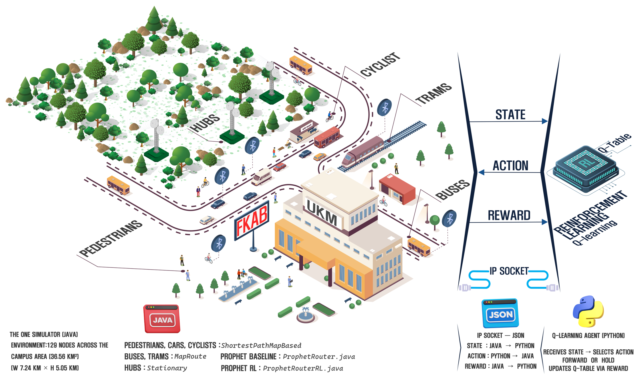
Figure 2.
Network topology of UKM-Bangi showing the spatial distribution of 129 nodes at the campus area (36.56 km2).
Figure 2.
Network topology of UKM-Bangi showing the spatial distribution of 129 nodes at the campus area (36.56 km2).
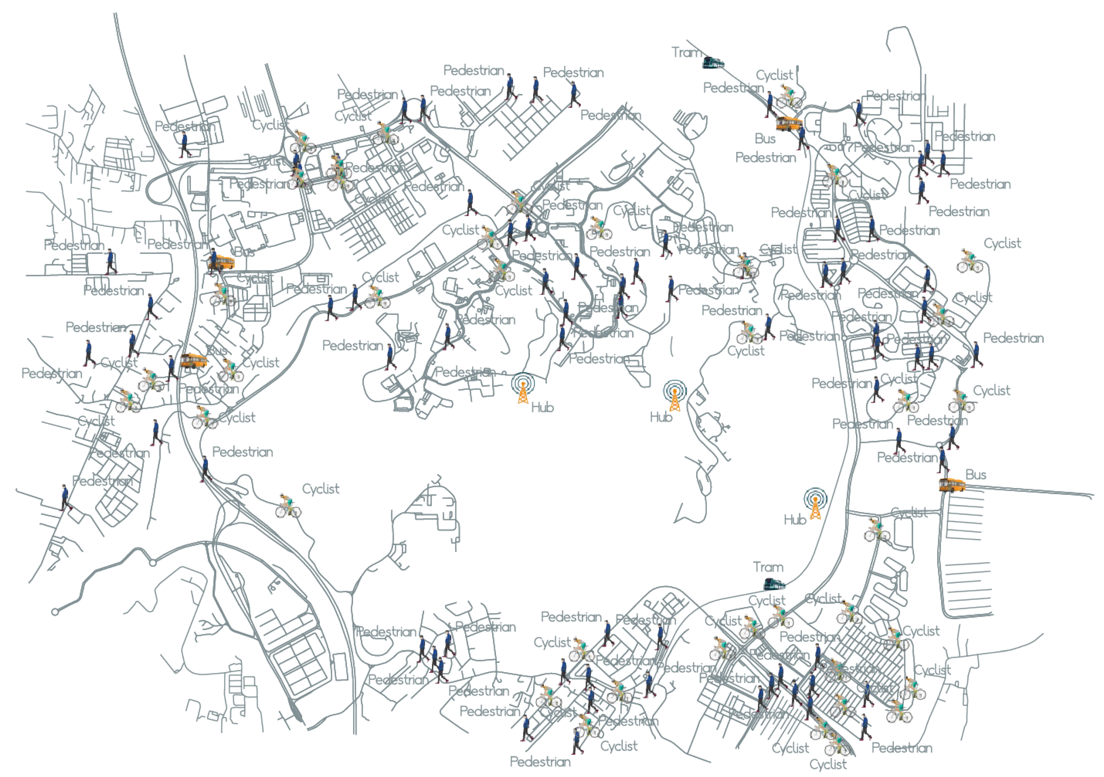
Figure 3.
Detailed two-stage routing decision process in ProphetRouterRL.
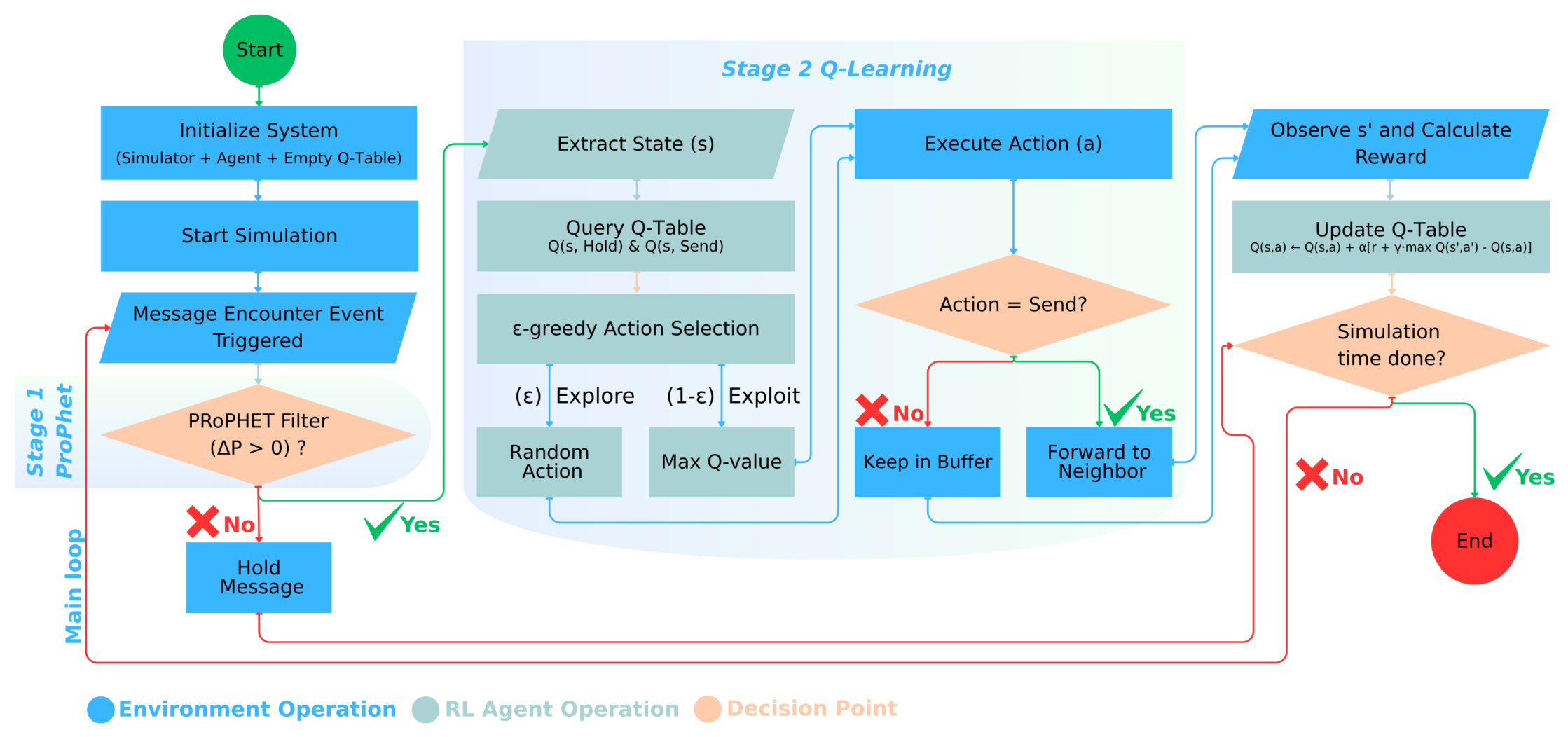
Figure 4.
Q-value evolution during 12-hour training.
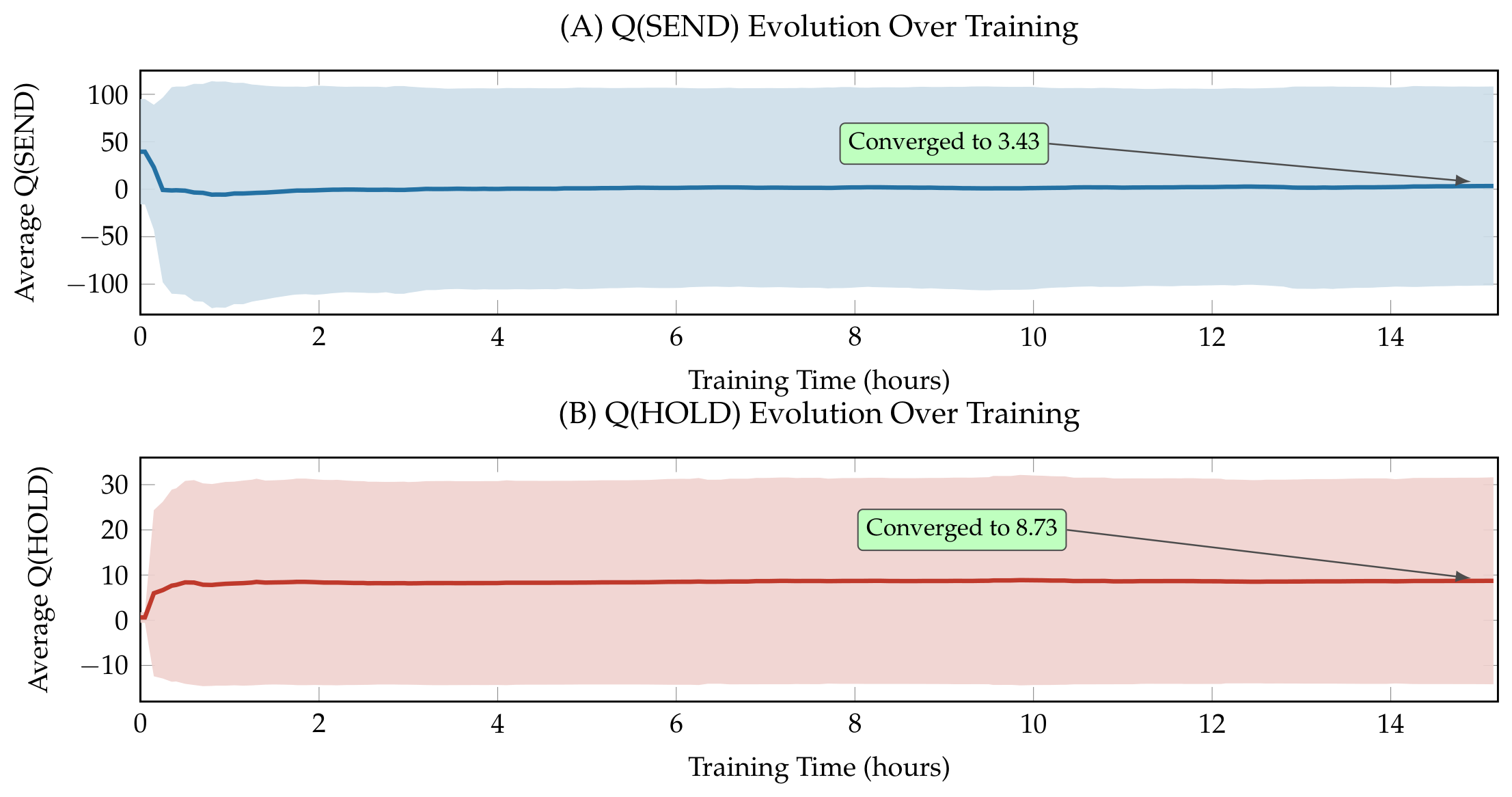
Figure 5.
Learning dynamics during 12-hour training.
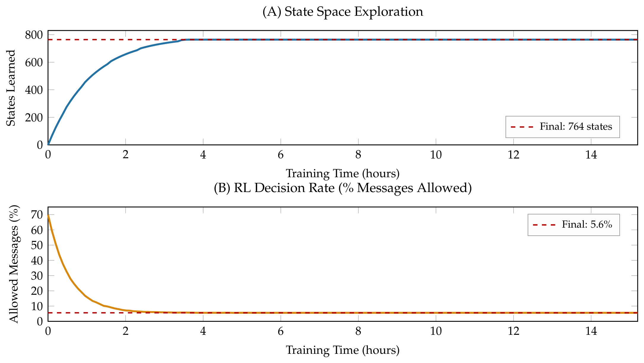
Figure 6.
Convergence stability analysis.
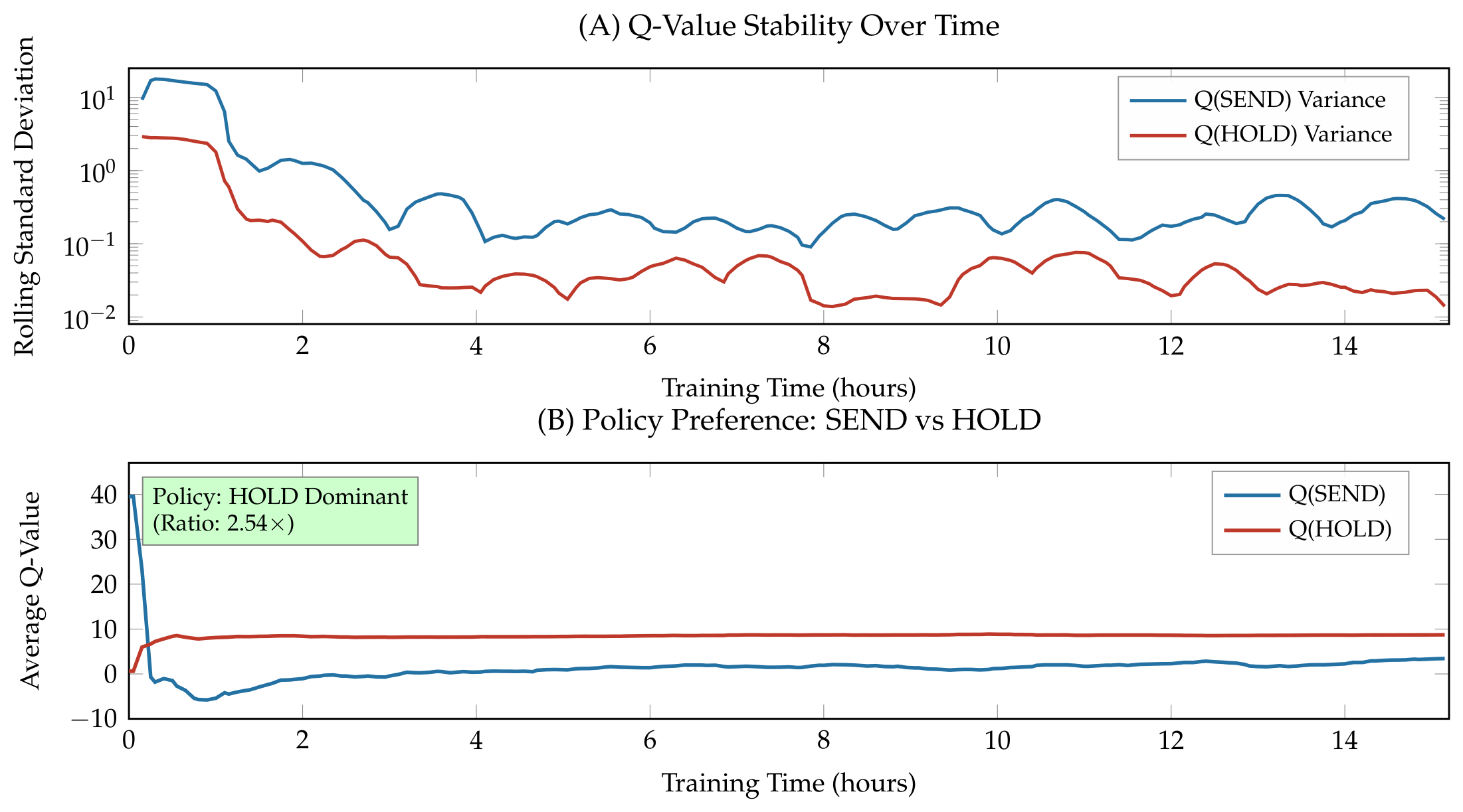
Figure 7.
Average Q-value () comparison between Fresh (12h Evaluation) and Mature Q-table (Trained 7d, Evaluated 12h) configurations.
Figure 7.
Average Q-value () comparison between Fresh (12h Evaluation) and Mature Q-table (Trained 7d, Evaluated 12h) configurations.
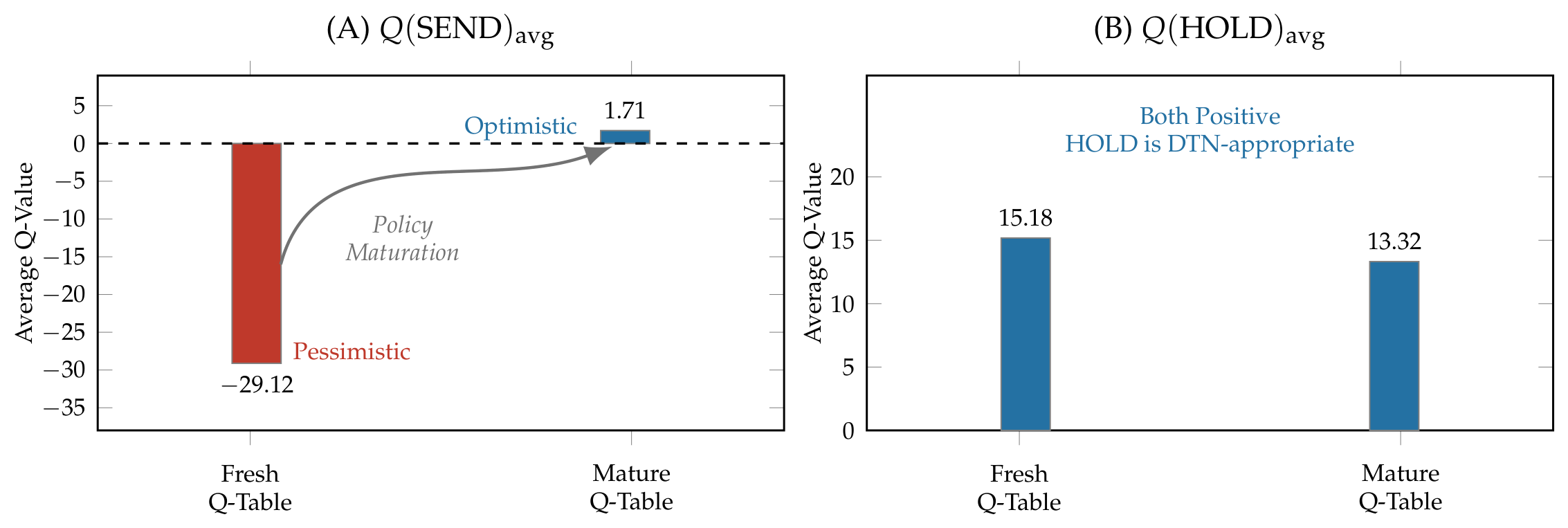
Figure 8.
Reproducibility validation across four independent runs using the mature Q-table.
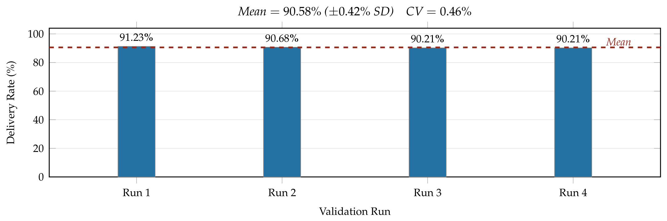

Table 1.
Comparison of RL-based approaches in DTN routing and related vehicular network applications.
Table 1.
Comparison of RL-based approaches in DTN routing and related vehicular network applications.
| Study | Learning Method | Network Type | Positioning Relative to this Work | Performance |
|---|---|---|---|---|
| Putela et al. (2025) [18] | Multi-armed bandit (UCB) | Generic OppNet (real-world traces) | Uses a bandit-based node score (proximity-to-destination reward plus degree centrality) rather than Q-learning or PRoPHET’s predictability estimation; PRoPHET is used only as an external comparison baseline (via RL-Prophet), not as a mechanism the protocol builds on | Reported higher delivery ratio and lower latency than Direct Delivery, Spray-and-Wait, and RL-based baselines on real-world contact traces |
| Rezaei & Derakhshanfard (2025) [11] | Q-learning (tabular) | Generic DTN | Uses RL to recompute PRoPHET’s delivery-predictability criterion itself, with a compact state (a categorical encounter-based state with five possible values) and a fractional-copy action space (0, 1, , or copies) - a multi-copy design point rather than a binary forward decision | Reported improvements in delivery and latency over PROPHET across several parameter sweeps |
| Schindlegger & Hupperich (2026) [13] | Q-learning (tabular) | Generic OppNet | Spray-Learn-Wait extends the spray-and-wait lineage with movement-based clustering and Q-learning, comparing against PRoPHET only as one of three established baselines rather than building on it | Reported gains in delivery and overhead over PRoPHET, accompanied by increased latency, across the tested node densities |
| ProphetRouterRL (This Work) | Q-learning (tabular) | Heterogeneous V2X DTN | Retains GRTR as an eligibility gate and uses a compact contextual state for the subsequentsend/holddecision | Evaluated against conventional PRoPHET in this work |
Table 2.
Node Type Characteristics
| Node Type | Nodes Count | Velocity | Buffer Size | Mobility | Interface |
|---|---|---|---|---|---|
| Pedestrians (p) | 40 | 0.6–1.3 m/s | 10 MB | ShortestPath | BT |
| Cyclists (w) | 40 | 3.5–6.0 m/s | 15 MB | ShortestPath | BT |
| Cars (c) | 40 | 3.5–12.0 m/s | 20 MB | ShortestPath | BT |
| Buses (b) | 4 | 10.0–15.0 m/s | 50 MB | MapRoute | BT+HS |
| Metro Trains (t) | 2 | 7.0–18.0 m/s | 150 MB | MapRoute | BT+HS |
| Static Hubs (h) | 3 | 0 | 150 MB | Stationary | BT+HS |
| Total | 129 | — | — | — | — |
Notes: Interfaces (BT = Bluetooth, 250 kbps; HS = High-speed, 50 Mbps).
Table 3.
PRoPHET Protocol Parameters
| Parameter | Symbol | Value | Purpose |
|---|---|---|---|
| Initialization constant | 0.15 | Encounter impact magnitude | |
| Transitivity factor | 0.10 | Indirect information weight | |
| Aging constant | 0.75 | Temporal decay rate | |
| Time unit | — | 30 s | Aging granularity |
Table 4.
Overall Performance Comparison: ProphetRouterRL vs. Baseline PRoPHET (7-Day Simulation)
| Metric | Baseline | ProphetRouterRL |
|---|---|---|
| Delivery Rate | 46.47% | 93.12% (↑100.4%) |
| Msgs. Delivered* | 9,522 | 19,084 (+9,562) |
| Overhead Ratio | 545.68 | 330.91 (↓39.4%) |
| Avg. Latency (s) | 1,953 | 1,144 (↓41.4%) |
| Avg. Latency (min) | 32.6 | 19.1 (−13.5 min) |
Notes: Out of 20,494 messages created in both runs
Table 5.
Q-Learning Effectiveness Validation: Mature Q-Table (Trained 7d, Evaluated 12h) vs. Fresh Q-Table (12h Evaluation)
Table 5.
Q-Learning Effectiveness Validation: Mature Q-Table (Trained 7d, Evaluated 12h) vs. Fresh Q-Table (12h Evaluation)
| Metric | Fresh Q-Table | Mature Q-Table |
|---|---|---|
| Delivery Rate | 58.42% | 91.16% (↑56.0%) |
| Msgs. Delivered* | 853 | 1,331 (+478) |
| Overhead Ratio | 515.26 | 194.97 (↓62.2%) |
| Avg. Latency (s) | 1,541 | 1,041 (↓32.5%) |
| Hop Count (avg) | 4.52 | 3.31 (↓26.8%) |
Notes: Out of 1,460 messages evaluated in both configurations.
Disclaimer/Publisher’s Note: The statements, opinions and data contained in all publications are solely those of the individual author(s) and contributor(s) and not of MDPI and/or the editor(s). MDPI and/or the editor(s) disclaim responsibility for any injury to people or property resulting from any ideas, methods, instructions or products referred to in the content. |
© 2026 by the authors. Licensee MDPI, Basel, Switzerland. This article is an open access article distributed under the terms and conditions of the Creative Commons Attribution (CC BY) license (http://creativecommons.org/licenses/by/4.0/).
Copyright: This open access article is published under a Creative Commons CC BY 4.0 license, which permit the free download, distribution, and reuse, provided that the author and preprint are cited in any reuse.