

Submitted:
07 October 2026
Posted:
09 October 2026
You are already at the latest version
Abstract
Millimeter-wave communications at 60 GHz offer access to large contiguous spectrum but require accurate propagation models to support reliable system design, as path losses at these frequencies are strongly influenced by buildings, vegetation, balconies, and intervening obstacles. This paper presents path gain models for outdoor-to-balcony and outdoor-to-indoor fixed wireless access (FWA) links at 60 GHz, derived from an extensive measurement campaign conducted in Athens, Greece. Measurements were collected with a street-mast transmitter and receiving nodes placed on balconies or indoors, covering a range of non-line-of-sight (NLOS) geometries representative of residential FWA deployments. Two existing channel models are adapted, tested and shown to predict measured path gain with lower RMS error than existing 3GPP models. Link-budget calculations using the proposed models show that, under the stated assumptions, 60 GHz FWA can deliver gigabit-class service to balcony-mounted receivers at short residential ranges with a 400 MHz deployment bandwidth.
Keywords:
60 GHz
; fixed wireless access communications
; FWA
; path gain
; channel measurements
; mmWaves
; foliage
; outdoor-to-indoor
; outdoor-to-balcony
1. Introduction
Wireless communication systems are thriving due to the increased global demand for uninterrupted internet connectivity by various types of mobile devices. This surge in demand necessitates faster data services and a larger bandwidth, which is a primary objective of wireless providers aiming at enhancing frequency spectrum and coverage. To maximize the benefits of wireless networks, reliable coverage is essential, achievable through the development of accurate channel models for mmWave frequencies.
In recent years, extensive research has focused on presenting various models and measurements for this purpose [1,2,3,4,5,6,7,8,9]. Studies for the fifth generation (5G) systems have examined path loss factors such as antenna height, distance, and frequency [10,11,12]. Notable models include the alpha-beta-gamma model and the close-in model, supported by extensive experimental data [13]. Approaches like ray tracing [14,15] and empirical models [16] are well-regarded in propagation modeling. Ray tracing, despite needing detailed environmental data, predicts full impulse responses for various environments, considering factors like interior walls and vegetation. While empirical models reduce the need for complex programming, minimizing site-specific measurements remains valuable. An analytical model for universal path gain laws, addressing rooftop propagation, outdoor to indoor transitions, and foliage, has been introduced in [17]. Other high-frequency and mmWave channel models are provided in [18,19,20,21,22], including the EU-funded mmMAGIC and METIS projects.
This paper presents a measurement-based modelling framework for 60 GHz residential outdoor-to-balcony and outdoor-to-indoor FWA links, by adapting the universal path-gain laws of [17] to account for vegetation, balcony coupling, window penetration, and local street irregularities. The rest of the paper is organized as follows: Section 2 describes the 60 GHz channel sounder and measurement procedure, while Section 3 introduces the R4 and EA test sites and the above-/below-vegetation receiver configurations. Section 4 and Section 5 develop the proposed above- and below-vegetation path-gain models. Section 6 formulates the effective balcony/window transmission factor, and Section 7 reports the measured glass and window-boundary penetration losses. Section 8 validates the proposed models against the measurements and compares them with the corresponding 3GPP references. Section 9 examines the degradation of effective azimuth gain caused by angular dispersion, while Section 10 characterizes the temporal variability of the measured NLOS links through the temporal K-factor. Section 11 translates the propagation results into 90% coverage rate estimates for balcony-mounted FWA terminals. Conclusions are drawn in Section 12.
2. Measurements Setup
The purpose of our experiments was to develop an outdoor-to-balcony and outdoor-to-indoor channel model suitable for wireless systems operating at 60 GHz. This model will be beneficial for Fixed Wireless Access (FWA) systems, where the base stations are positioned at strategic street locations, such as lamp-posts or traffic lights, while the client receivers are located either outdoors on balconies or indoors near windows. The measurements were conducted utilizing the channel sounder depicted in Figure 1. It is developed by Nokia Bell Labs and consists of a transmitter (Tx) unit bearing an omnidirectional antenna and a receiver (Rx) unit bearing a directional horn antenna. The Rx antenna is mounted on a rotating platform (spinner) rotating at 300 rpm, collecting up to 702 samples per rotation with an angle step size of one degree. The spinner allows reception from all angles. The sounder operates at a frequency of Fc=60 GHz, and a bandwidth W=20 kHz. The directional Rx antenna has:
- A gain of 24.9 dBi,
- Half Power Beam Width (HPBW) 10° in azimuth and 9° in elevation,
while the omnidirectional Tx antenna has:
- a gain of 5 dBi and
- 30° HPBW in elevation.
Two test sites were selected for our experiments, both located at Residence Halls of the American College of Greece (ACG) near its main campus in Aghia Paraskevi, Athens, but embedded within the urban fabric. These sites are identified as Residence Building 4 (R4) and External Apartments (EA), as referenced throughout this paper and depicted in Table I. The locations represent a typical dense suburban environment in Athens, featuring three- to four-story buildings, small gardens separating neighboring structures, and relatively narrow streets compared to the height of the buildings. Medium-sized, moderately dense trees, often situated near the buildings, frequently obscure the lower floors in both height and width. Figure 2, Figure 3, Figure 4 and Figure 5 show the two streets containing the test sites, while Figure 6 shows the balconies of the two test sites.
The geometrical parameters of the measurement setup are depicted in Figure 7. The transmitter, representing a below-street clutter microcell, was mounted on a tripod at a fixed height Zm =3.5 m and in a region free from clutter. The receiver unit was placed in buildings on the opposite side of the street, on the balcony and then indoors, behind and close to the window, to assess penetration loss through the overall window structure, including the window glass. While the Rx unit remains fixed, the Tx unit (on its tripod) moves along the street, covering a total distance of 250 to 300 meters, as illustrated in Figure 2 and Figure 4. The received power is recorded by the sounder at hundreds of Tx positions, each with known Rx-Tx distances. The corresponding path gain is then calculated for each position. These measurements are designed to evaluate oblique incidence angles as well as Non-Line of Sight (NLOS) conditions for FWA, using street furniture and considering the impact of vegetation or other obstacles on signal propagation.
3. Measurement Locations
Measurements were performed in the locations, and according to the scenarios that are mentioned in Table 1. In addition to the outdoors/indoors distinction, two more scenarios were studied:
- The Rx unit below foliage.
- The Rx unit above the tree line.
The R4 flats include a large lounge area furnished with standard campus furniture. The balconies consist of a combination of metal railings and modern metalized glass panels. The street is lined with tall trees on both sides, and two large Mediterranean pine (Pinus Halepensis) stand in front of the building. During the measurement period, the road experienced substantial traffic. The EA flats are equipped with similar campus-style furniture; however, their balconies use older plain glass panels combined with metal railings. Trees are also present along both sides of the road, though they are generally smaller than those on the R4 street. Medium-sized olive trees are located in front of the building. Traffic was light during our measurements at this site. In both cases, there was no wind during the measurements, ensuring that tree motion did not influence the channel conditions.
4. Theoretical Path Gain for Remote Above Vegetation and Base Antenna Mast Below
This case is represented in the side view of Figure 7, where the Rx is located on the upper balcony. The path gain model, “Above Vegetation” is derived by applying reciprocity to equation 22 of [17], exchanging the roles of base station and terminal so that the elevated balcony Rx takes the place of the above-clutter base, and adopting the clutter-penetration structure of [17] (eq. 20) for the below-clutter Tx end, which contributes the local vegetation-depth term and the ground-reflection factor . Two additional terms are incorporated to match the present geometry: the back-wall reflection , supported by the measured angular power spectrum, and the atmospheric absorption factor , yielding equation 1 for path gain when terminal on balcony is above vegetation:
where λ is the wavelength, is the height of the receiver Rx, is the clutter height or the top of the trees, is the height of the mast where the transmitter is mounted, κν is the absorption of the diffuse clutter in Np/m (the foliage in this case), Atmospheric absorption at 60 GHz is accounted for using a 15 dB/km 0.0035 Np/m (power coefficient), [23], and Γg is the ground reflection coefficient. The term Γw is introduced to account for signal reflections by the balcony’s structural elements such as walls, ceiling, railing, etc. The term Teff is used here as a generalized effective transmission coefficient for the receiver-side boundary region. In [17], Teff is introduced as an effective aperture or boundary transmission coefficient. In the present measurements, however, the Rx is located on a recessed balcony, and therefore Teff is interpreted as a site-specific coupling coefficient that accounts for the balcony aperture and associated structural screening. For indoor measurements, the additional window penetration and indoor propagation losses are introduced separately, as described below and further detailed in Section 6. This interpretation preserves the structure of [17] while adapting it to the measured balcony-to-street geometry.
In addition to the “Above Vegetation (AV)” model of eq. 1, we also consider an adapted form of the “Urban Canyon to Terminal on a Cluttered Sidewalk” model presented in [17] (Sec. VII). That model addresses a related reciprocal geometry, where an elevated rooftop/lamppost base illuminating a terminal low on the sidewalk further down a tree-lined street. The path gain has a guided and an unguided term. The guided term describes multi-bounce propagation down the street canyon, decaying as r⁻²·⁵ with a range-growing vegetation loss, while the unguided term of equation 19 of [17] is the lowest-order path penetrating the roadside clutter from the side, decaying as r⁻⁴ with only the local foliage-depth loss. As the two dominate under opposite tree densities, they are merged by a maximum operator:
This formulation explicitly includes a range-dependent vegetation attenuation, which agrees with the non-uniform street and vegetation topology of our test sites and provides an alternative model for comparison with eq. 1. Adjusting equation 41 of [17], for the total path gain, to our geometry gives the following:
where:
- ○
- ○
- ○
Furthermore: PAV is the term given by eq. 1; w is the street (canyon) width; κv is the attenuation rate of the vegetation, in Np/m; ρv is the tree volume density along the street, i.e., the fraction of the canyon volume below the base station occupied by trees (0 ≤ ρv ≤ 1); dv is the vegetation depth near the terminal, i.e. the foliage thickness the path crosses close to the receiver; ds is the standoff distance from the base antenna to the foliage/scattering region near the terminal; L is the wall-loss parameter of the canyon walls; L₁ is the same wall-loss parameter inflated by foliage and finally, accounts for the excess absorption higher-order reflections suffer crossing vegetation. The wall and ground reflection coefficients Γw and Γg are the same terms as in eq.1. Notice in the equations above that there are two factors that relate to foliage absorption:
- The factor is the local penetration loss, common to both terms, which does not depend on range r.
- The term is the distributed vegetation loss accumulated along the guided path and grows with range because higher-order canyon reflections travel farther through foliage.
Equation 2b does not include the explicit direct term Pdirect of equation 41 of [17]. This reduced form is used because the retained above-vegetation NLOS dataset does not provide a consistently dominant or reliably parameterized straight-through-foliage component; short-range links for which such a component may dominate are excluded from the NLOS model comparison. Therefore, eq. 2b is treated as a reduced canyon-composite reference model, retaining the guided/unguided cluttered-sidewalk contribution and the above-vegetation term, but not the explicit direct-ray contribution. The applicability of both models of eq. 1 and eq. 2b to the measured data is examined in Section 8.
For the indoor measurement configuration above vegetation, all the previous path gain models are retained, while the effective transmission coefficient is modified to account for both boundary penetration and indoor propagation losses as in [17]. Specifically, the effective transmission coefficient is expressed as:
where represents the transmission through the balcony/window interface, is the effective indoor attenuation coefficient (Np/m), and is the distance between the boundary and the receiver inside the room following the method of [17], where wall penetration and indoor losses are treated as separate multiplicative factors. More details are given in section 6.
5. Theoretical Path Gain When Both Terminals Are Below Treetops
This case corresponds to the R4 test site (Table I). The rotating receiver is located on a balcony, or indoors below the tree canopy, while the transmitter is mounted on the street-level mast at Zₘ = 3.5 m. When both the Tx and Rx are below the treetops, the above-vegetation mechanism of the previous section, (in which the signal would travel upward to the canopy, scatter across it, and scatter again down to the receiver), incurs prohibitive attenuation and is therefore neglected. The dominant contribution instead follows a near-horizontal path: the signal propagates along the street from the transmitter on mast, reaches the vegetation immediately outside the balcony, penetrates the foliage from the side, and finally crosses the balcony and window interface into the room (when the Rx is indoors). This is precisely the suburban foliage-penetration scenario of [17] (eq. 20), extended to an indoor terminal as in equation 21 of [17]. Adapted to the present balcony geometry, the "Below Vegetation" path gain is:
where κv is the absorption due to the foliage in Np/m; dv is the vegetation depth (foliage thickness) between the street and the Rx; ds is the standoff distance between the Tx and the nearest point of the foliage boundary (Figure 7); and are the ground and wall power reflection coefficients respectively. In the present balcony geometry, represents receiver-side balcony/building reflections, while represents an effective ground-reflection contribution that may be reduced by intervening vegetation and street-level clutter. Finally, following equation 21 of [17], accounts for transmission through the balcony/window interface and for indoor propagation loss over depth dᵢₙ, with Teff constructed as in Section 6.
6. Penetration Loss into Balcony and Interior
To the best of our knowledge, this is one of the first measurement-based attempts to explicitly parameterize the combined balcony/window coupling loss for 60 GHz residential FWA links. The balcony is treated as an additional boundary to penetrate, so that the effective transmission coefficient follows from equation 64 of [17]:
where = 1.5m is the vertical distance between the balcony railing and balcony ceiling and = 1m which is the depth of placement of the Rx on the balcony. The parameter , accounts for the fact that the railing and the remaining balcony structures do not act as the high-loss walls assumed in [17] (eq. 64). At the EA site, the balcony is relatively open, consisting of older plain glass panels and sparse metal railings, which do not strongly screen the incident 60 GHz field. A good fit was obtained for corresponding to a total . By contrast, at the R4 site the railings comprised tinted, high-loss glass, for which the high-loss-wall assumption of [17] (eq. 64) holds, so no correction is required (, ).
Using equation 64 of [17], for a receiver inside the room, the effective boundary transmission coefficient is modeled as follows:
where is the glass loss, din (~1 m) is the depth of the Rx inside the room and w1 × w2 are the balcony door dimensions. The total Teff is thus dependent on location of the remote unit:
7. Glass and Window-Boundary Penetration Measurements
Before starting the measurements described above, the penetration loss associated with the window boundary was evaluated during calibration of the channel sounder. The Tx unit was placed on a balcony, while the Rx unit was positioned behind the window glass at a distance of 1 meter, with both units aligned at the same height. Although the short Tx–Rx separation ensures that the window glass is the dominant contributor, the measured loss inherently includes the complete Rx-side region, (balcony structure, window frame, and the immediate indoor surroundings), and is therefore representative of the effective boundary transmission encountered in the deployment scenarios of Section 4, Section 5 and Section 6. In our experiments, we encountered two types of glass:
- Single plain glass: found only on the 4th floor of building EA.
- Double-glazed metallized glass: found on both floors of building R4 and the 3rd floor of building EA.
The exact specifications of these glasses are unknown. However, the measured peak (best-angle) loss ranged from 3 dB for the single plain glass up to 40 dB for the double-glazed metallized glass, as illustrated in Table 2. These values should be interpreted as in-situ window-boundary insertion losses rather than intrinsic material attenuation coefficients of the isolated glass panes.
Our findings are in very good agreement with these reported in [24,25,26,27] and they highlight that 60 GHz communication through metalized windows commonly used in modern buildings may be highly challenged. Such significant attenuation emphasizes the importance of accounting for window-glass type when deploying millimeter-wave systems. In the present measurements, apartments with double-glazed metallized windows produced measurable signals only when the receiver was placed on the balcony; indoor reception was below the sensitivity of the channel sounder. This corresponds to an effective path gain of approximately PG < -160dB, implying received-power levels too low for reliable practical communication.
8. Measured Results and Discussion
Figure 8 depicts the path gain versus range for all the measured links, both outdoor-to-balcony (O2B) and outdoor-to-indoor (O2I), for the two test sites. The following measurements were excluded from our final dataset:
- All measurements corresponding to LOS links.
- The indoor measurements performed on building R4 and on the 3rd floor of building EA because of the large penetration loss (PG < -160dB) through double-glazed metallized windows as described in the previous section.
- Measurements for which the combined effect of antenna height difference and Tx–Rx separation resulted in a vertical misalignment exceeding the elevation HPBW of the antennas.
Although Figure 8 shows two main data clusters, O2B in blue and O2I in red, part of the O2B dataset overlaps with the O2I measurements. These points correspond to the R4 site, where the combined attenuation introduced by the metallized-glass balcony railings and the below-vegetation Rx placement reduces the received power to levels comparable to indoor reception.
Figure 9 depicts the difference between indoors and outdoors reception for the EA test site where the receiver is above vegetation. The two datasets are clearly separated with a Mean Absolute Difference (MAD) of approximately 18 dB caused by the combination of balcony, walls and plain glass windows. As stated before, indoors reception was possible only through the plain glass windows of the 4th floor.
Figure 10 depicts the outdoor-to-balcony (O2B) measured path gain for sites EA-I and EA-II (above vegetation), together with the predictions of eq. 1 (green line) and eq. 2b (purple line). The 3GPP Urban Microcell (UMi) Street Canyon NLOS model [18] is also included as a standardized benchmark. The UMi model was selected as the primary standardized reference for outdoor links because the receiver height in our experiments is close to the nominal UMi base-station height of 10 m, and the measurements were conducted along a narrow urban street. As shown in Table 3, eq. 1 provides the lowest RMS error, 4.3 dB, compared with eq. 2b and the 3GPP UMi model. However, the 1 dB improvement over the 3GPP Umi model is relatively modest.
Figure 11 shows the R4 O2B measurements for the below-vegetation case together with the model prediction of equation 4 and the 3GPP UMi Street Canyon NLOS reference. In contrast to the EA above-vegetation case, where the 3GPP UMi model produced an RMS error comparable to the proposed models, its performance degrades substantially for R4, yielding an RMS error of 11.71 dB compared with 3.13 dB for eq. 4. This difference indicates that, when both terminals are below the tree line, propagation is governed primarily by local lateral foliage penetration, with additional receiver-side balcony/building interactions and site-specific street clutter, none of which are explicitly represented in the generic UMi formulation. The result therefore supports the need for specialized below-vegetation models for residential FWA deployments, while also showing that standardized models should be used with caution when the measurement geometry departs from their nominal street-canyon assumptions.
Figure 12 compares the outdoor-to-indoor (O2I) above-vegetation measurements, with the receiver located indoors behind a single-pane/plain-glass window, against the proposed models and two 3GPP references. The outdoor 3GPP UMi curve provides an optimistic upper reference because it omits O2I penetration, while the 3GPP low-loss O2I model [18] (Table 7.4.3-2) provides a conservative lower reference; together, they approximately bracket the measured data but with large RMS errors of 15.6 dB and 11.1 dB, respectively.
In contrast, the two proposed formulations provide substantially better, and almost equivalent, agreement, indicating that the balcony/window coupling and vegetation-affected propagation should be represented explicitly.
Table 3 depicts the values of the various parameters of the path gain models. Notice that the foliage absorption coefficient is not treated as a universal constant but is assigned according to the propagation mechanism represented by each model. It can be seen in Table 3 that for the above-vegetation models of equations 1 and 2b, we used as an effective power-extinction coefficient for sparse, spatially discontinuous roadside vegetation, where the dominant path grazes the upper canopy and partly propagates through gaps between tree crowns rather than through a continuous foliage block. This value is consistent with low effective attenuation rates reported for some mmWave foliage measurements, such as the 73 GHz foliage rate of approximately , (corresponding to 0.4 dB/m) [4].
More generally, measurements at 26–32 GHz, [28,29], show that the attenuation induced by vegetation, foliage and along rows of trees is highly non-uniform, supporting the use of a geometry-dependent effective foliage absorption coefficient. For the below-vegetation model of eq. 4, however, the dominant mechanism is direct lateral penetration through the receiver-side foliage, with no volumetric filling factor in the expression. A larger value, , is therefore used for eq. 4, representing a direct through-crown power-extinction rate. This value is consistent with the lower range of the values given in [30], assuming canopy depths toward the upper end reported (~7–8 m).
The reflection terms were fixed as physically constrained effective parameters rather than jointly optimized with the model fit. Their nominal values were guided by the measured angular power spectra of Figure 13 and by reported mmWave reflection coefficients for relevant ground and building surfaces [31,32,33]. Sensitivity tests in which and were varied from 0.3 to 0.7 resulted in RMS-error variations of approximately , while the relative model performance and the main conclusions remained unchanged. Accordingly, nominal values of = were retained for the above-vegetation O2Β case. For eq. 4, was retained, whereas represents the substantially weaker local ground return through intervening vegetation and street-level clutter, consistent with reported reductions in effective under-canopy ground reflectivity [31]. The dimensionless amplitude coefficient is treated as an effective glazed-boundary transmission parameter. At 60 GHz, the 3GPP TR 38.901 standard multi-pane glass loss of 14 dB corresponds to . More broadly, reported 60 GHz measurements [32,33,34,35] span approximately –0.8 for bare smooth glass at normal incidence, –0.5 when incidence angle and deployed glass configurations are considered, and below 0.03 for metallized glazing, confirming the strong dependence on glazing structure and propagation geometry. Accordingly, , which also yielded the best agreement with the present measurements, was retained as the nominal value. Sensitivity tests over resulted in RMS-error variations of at most approximately , without changing the relative model performance. Nevertheless, values below 0.1 and above 0.35 severely affected the fitting of all tested models.
9. Azimuth Gain Degradation
In rich scattering environments, the received signal arrives at the antenna from multiple directions rather than from a single dominant angle.
Figure 13 compares the measured average power azimuth spectrum (PAS) with a synthesized horn response (dashed) of the same nominal half-power beamwidth, aligned with the strongest received direction, which does not necessarily coincide with the Tx-Rx direction, i.e., the true main lobe. The dashed lobe provides a single-arrival reference, in the sense that if one specular component dominated the channel, the measured PAS would closely follow this beam pattern. Instead, the spectra extend well beyond the reference lobe showing that significant power arrives from multiple azimuth directions. Since this angular spread exceeds that expected from the receive beamwidth alone, it reflects channel-induced multipath, consistent with the vegetation scattering and facade/building backscatter mechanisms considered in this work. The effect is observed for both balcony and indoor receivers, and is stronger indoors, where wall/window penetration and boundary reflections produce more diffuse spectra with reduced lobe contrast.
This angular spread causes a mismatch between the antenna’s designed radiation pattern and the spatial distribution of the incoming multipath components. As a result, only a fraction of the total received power is captured within the antenna’s main beam, while the remaining power arrives from other directions and experiences reduced antenna gain. Consequently, the effective antenna gain is lower than the nominal gain, leading to reduced received signal power. This effect is shown in Figure 14, depicting the measured CDFs of the effective azimuth gain for indoors and outdoors receiver placements, each bounded by its 90% Dvoretzky–Kiefer–Wolfowitz (DKW) confidence band [36,37] and overlaid with a log-normal fit (blue dotted lines). The two distributions are clearly separated: the effective azimuth gain exceeded in 90% of cases is 9.4 dBi indoors and 10.2 dBi outdoors, both well below the nominal antenna gain of 14.9 dBi, corresponding to reductions of 5.5 and 4.7 dB, respectively. The reduction is attributed to angular dispersion of the received power in the scattering environment, which is more pronounced for indoor terminals owing to additional facade and interior scattering. The two 90% bands have a Wasserstein-1 distance (average horizontal separation) of 1.5 dBi. Notice that the effective azimuth gain is evaluated over both LOS and NLOS links as it quantifies the realizable gain across the entire deployment. Retaining both link types therefore provides a deployment-wide gain statistic representative of terminals distributed across LOS and NLOS conditions alike.
10. Temporal Variation
Temporal variation of the received signal at each fixed link, generally arising from wind-blown vegetation, moving vehicles, pedestrians, and similar environmental dynamics, is characterized by the temporal K-factor. The corresponding values were computed for all test sites using the approach of [36,40]. Physically, the temporal K-factor expresses the ratio between the dominant, relatively stable signal component and the diffuse time-varying component caused by moving scatterers such as wind-blown vegetation, [41]. A high temporal K-factor therefore indicates a more stable link with limited short-term fading, whereas a low value indicates stronger temporal fluctuations and fading-margin requirements. Figure 15 shows the measured CDF of the temporal K-factor for each test site, with the 90% confidence band [37] shaded and a log-normal fit overlaid. The R4 distribution lies consistently to the left of the EA distribution, consistent with the more favorable propagation conditions at EA, where traffic density and vegetation obstruction were lower. The separation corresponds to a Wasserstein-1 distance of 3.6 dB, with a median gap of 3.1 dB. The log-normal model fits the EA distribution well but departs noticeably from the R4 distribution; while partly attributable to the smaller R4 usable sample, this departure is also consistent with R4 aggregating more heterogeneous link conditions, for which a single log-normal is an incomplete description. The K-factor is evaluated over NLOS links only, since LOS links contain a strong, stable component that inflates the K-factor and is not representative of the scattering-limited NLOS regime of interest in both test sites.
11. Achievable 90% Coverage Rate
The preceding sections characterized the path gain, the azimuth-gain degradation and the temporal fading of the 60 GHz channel. In this section, we translate those propagation results into the metric most directly relevant to system design: the data rate that can be offered to 90% of users. Using the methodology that was presented in [36,40], we define the 90% coverage capacity as the Shannon rate that is met or exceeded by 90% of the user-terminal locations served by a base station at a given range r and is calculated by:
where B is the system bandwidth and SNR is the linear signal-to-noise ratio at the receiver. Although the channel sounder used in our campaign operated over a narrow 20 kHz bandwidth, the capacity is evaluated for a representative deployment bandwidth of B = 400 MHz, consistent with the large contiguous spectrum available in the 60 GHz band. The signal-to-noise ratio (SNR) is obtained from a standard link budget. With all quantities expressed in logarithmic scale, the SNRdB (dB) at the receiver is:
where PTx is the transmitted power, GTx and GRx are the Tx and Rx antenna gains respectively, PG (r) is the path gain predicted by equations 1, 2b or the 3GPP UMi reference model and M90 is the common engineering margin that secures 90% coverage (discussed below). The receiver noise power is:
where −174 dBm/Hz is the thermal noise spectral density kT0 at T0 = 290 K, J/K is the Boltzmann constant and NF is the receiver noise figure in dB. The parameters used for the calculations of the 90% capacity are: PTx = 27dBm, GTx = 5 dBi, GRx = 15 dBi, NF = 7 dB and M90= 8.5 dB.
SNRdB(r) = PTx + GTx + GRx + PG (r) − M90 − N
N = −174 + 10 log10(B) + NF
The margin is used as a common engineering margin providing a representative approximation of the additional link budget required for 90% location coverage. Following [36,40], it combines three independent location-dependent contributions: (a) large-scale shadow fading, dB, obtained as the standard deviation of the residuals between the measured NLOS path gain and the model of eq. 1 after removal of the mean residual; the corresponding uncentered RMS error, including the mean residual of dB, is 4.26 dB, as reported in Table 3; (b) effective azimuth-gain degradation, with dB and dB obtained as the mean and standard deviation of the per-link difference between nominal and effective azimuth gain, the latter calculated from the peak-to-azimuth-average received-power ratio as in [36]; and (c) model uncertainty, dB, associated with the finite measurement set used to estimate the parameters of eq. 1. Assuming independence and approximately Gaussian variations in the dB domain, the 90% margin is, 8.5 dB, where is the one-sided standard-normal quantile for 90% coverage. The same is applied to all curves in Figure 16 so that their differences reflect the underlying path-gain predictions rather than model-specific margin assumptions. So, the 90%-coverage interpretation applies directly to eq. 1, from which is derived while curves for models with larger residual errors are retained as common-margin comparison references. The temporal K-factor of the previous section is not included in , since represents spatial location-to-location variability, whereas the K-factor characterizes temporal fluctuations at a fixed link.
The 90% coverage capacity is calculated for balcony-mounted receivers, which the path gain analysis of the preceding section identified as the preferred deployment location for FWA systems operating at 60 GHz. Figure 16 shows the received SNR and the corresponding downlink-rate estimates for two representative receiver clearances above the vegetation clutter and at 60 GHz. An indicative received SNR threshold of −6 dB is adopted as a practical lower operating limit. This value is consistent with the low-spectral-efficiency QPSK operation supported by the LTE CQI framework, in which CQI selection targets a transport-block error probability not exceeding 10% [42,43]. However, the precise operating threshold depends on the receiver implementation, channel conditions, and target block error rate. The Shannon rate curves are therefore truncated below this threshold, as the rates predicted by the ideal Shannon expression may not be realizable. Furthermore, a separate 3 dB implementation gap accounts for non-ideal coding and receiver performance by reducing the SNR used in eq. 8 by 3 dB. The −6 dB operating threshold is applied to the received SNR before this implementation adjustment.
The capacity results for 90% location coverage, shown in Figure 16, indicate that the 60 GHz band can deliver gigabit-class service to balcony-mounted FWA terminals under NLOS conditions for receivers above the vegetation clutter. The two receiver-clearance cases quantify the sensitivity of the predicted downlink performance to the assumed receiver height above the clutter. For the cases shown, the estimated downlink rate at 40 m ranges from approximately 0.9 to 1.3 Gbps, while the dB operating threshold is reached at distances of approximately 90–108 m, depending on the path-gain model and receiver clearance. These results suggest that a single base station per street may provide service-grade rates across the typical inter-building distances of a residential neighborhood under the assumed downlink parameters, including 27 dBm transmit power, an assumed conservative total receive-antenna gain of 15 dBi, and 400 MHz bandwidth. These rates should be interpreted as capacity-based estimates under the stated link-budget assumptions, including the operating threshold and implementation gap, rather than as protocol-level throughput predictions.
12. Conclusions
This paper presented 60 GHz outdoor-to-balcony and outdoor-to-indoor FWA measurements in residential balcony-to-street geometries and proposed path-gain models adapted to above- and below-vegetation propagation. Two findings carry direct deployment implications for similar residential settings. First, indoor reception through windows is highly sensitive to glass type: while single plain glass may permit measurable indoor links, modern double-glazed metallized energy-efficient windows can introduce losses of several tens of decibels and may render indoor 60 GHz reception impractical. Reliable FWA service in such environments should therefore be primarily provisioned through outdoor or balcony-mounted terminals rather than relying on in-room receivers behind glass. Second, the results reinforce the importance of locally clutter-free base-station placement. The strong dependence of path gain on vegetation and street-level obstruction, together with the degradation of the generic UMi model below the tree line, shows that the base-station side should maintain unobstructed angular visibility as far as possible for the proposed models and link-budget predictions to remain valid. Under the stated link-budget assumptions, incorporating a −6 dB operating-SNR threshold and a 3 dB implementation gap yields 0.9–1.3 Gbps at 40 m for 90% of balcony receiver locations over a 400 MHz bandwidth, with the −6 dB operating threshold reached at roughly 90–108 m depending on the model and receiver clearance.
These results support gigabit-class downlink operation at short residential ranges, while the receiver’s SNR operating threshold will limit coverage at larger distances. Uplink performance requires a separate link budget and may be lower when the terminal is subject to more restrictive transmit-power limits. The permissible transmit power depends on antenna gain, equipment category, and applicable conducted-power and EIRP limits. For example, the US Federal Communications Commission (FCC) regulations for the 57–71 GHz band generally specify a maximum average Equivalent Isotropically Radiated Power (EIRP) of 40 dBm and a maximum peak conducted power of 27 dBm, while the corresponding European harmonized conditions specify a maximum EIRP of 40 dBm, an EIRP density of 23 dBm/MHz, and a maximum antenna-port power of 27 dBm for general wideband data equipment [44,45]. Consequently, the applicable limits ultimately depend on the equipment category, antenna configuration, deployment type, bandwidth, and regional authorization framework.
Author Contributions
Conceptualization, R.V., D.C., J.D., J.S., M.R. and R.F.; methodology, R.V., D.C., J.D., J.S., M.R. and R.F.; software, G.V., M.H.T., I.G., D.C., J.D., J.S., M.R. and R.F.; validation, G.V., I.B., S.L., D.C., J.D.; formal analysis, G.V. and M.H.T.; investigation, M.H.T., I.G., M.S. and G.V.; resources, C.P., D.C., J.D., J.S., M.R. and R.F.; data curation, G.V., M.H.T., I.G. and M.S.; writing—original draft preparation, G.V. and M.H.T.; writing—review and editing, S.L., C.V., I.B. and D.C.; visualization, G.V., M.H.T. and C.V.; supervision, R.V. and C.P.; project administration, C.P. All authors have read and agreed to the published version of the manuscript.
Funding
Part of this work was supported by ANID FONDECYT Regular Project 1250951 and ANID CCTVal Project CIA250027.
Data Availability Statement
Data is available upon request from the authors.
Conflicts of Interest
The authors declare no conflicts of interest.
Abbreviations
The following abbreviations are used in this manuscript:
| ACG | American College of Greece |
| CDF | Cumulative Density Function |
| DKV | Dvoretzky–Kiefer–Wolfowitz |
| EA | External Apartments |
| EIRP | Equivalent Isotropically Radiated Power |
| FCC | Federal Communications Commission |
| HPBW | Half Power Beam Width |
| LOS | Line of Sight |
| MAD | Mean Absolute Difference |
| NLOS | Non-Line of Sight |
| O2B | Outdoors to Balcony |
| O2I | Outdoors to Indoors |
| PAS | Power Azimuth Spectrum |
| R4 | Residence Building 4 |
| Rx | Receiver |
| SNR | Signal-to-Noise Ratio |
| Tx | Transmitter |
| UMi | Urban Microcell |
References
- N. T. T. Docomo, “5G Channel Model for bands up to100 GHz’’, 5G workshops, 2015.
- K. Haneda et al., “Indoor 5G 3GPP-like channel models for office and shopping mall environments,” 2016 IEEE International Conference on Communications Workshops (ICC), Kuala Lumpur, Malaysia, 2016, pp. 694-699. [CrossRef]
- S. Deng, M. K. Samimi and T. S. Rappaport, “28 GHz and 73 GHz millimeter-wave indoor propagation measurements and path loss models,” 2015 IEEE International Conference on Communication Workshop (ICCW), London, UK, 2015, pp. 1244-1250. [CrossRef]
- T. S. Rappaport and S. Deng, “73 GHz wideband millimeter-wave foliage and ground reflection measurements and models,” 2015 IEEE International Conference on Communication Workshop (ICCW), London, UK, 2015, pp. 1238-1243. [CrossRef]
- K. Haneda et al., “5G 3GPP-Like Channel Models for Outdoor Urban Microcellular and Macrocellular Environments,” 2016 IEEE 83rd Vehicular Technology Conference (VTC Spring), Nanjing, China, 2016, pp. 1-7. [CrossRef]
- S. Nie, G. R. MacCartney, S. Sun and T. S. Rappaport, “72 GHz millimeter wave indoor measurements for wireless and backhaul communications,” 2013 IEEE 24th Annual International Symposium on Personal, Indoor, and Mobile Radio Communications (PIMRC), London, UK, 2013, pp. 2429-2433. [CrossRef]
- K. Haneda, N. Omaki, T. Imai, L. Raschkowski, M. Peter and A. Roivainen, “Frequency-Agile Pathloss Models for Urban Street Canyons,” in IEEE Transactions on Antennas and Propagation, vol. 64, no. 5, pp. 1941-1951, May 2016. [CrossRef]
- G. R. MacCartney and T. S. Rappaport, “Study on 3GPP rural macrocell path loss models for millimeter wave wireless communications,” 2017 IEEE International Conference on Communications (ICC), Paris, France, 2017, pp. 1-7. [CrossRef]
- T. S. Rappaport, G. R. MacCartney, M. K. Samimi and S. Sun, “Wideband Millimeter-Wave Propagation Measurements and Channel Models for Future Wireless Communication System Design,” in IEEE Transactions on Communications, vol. 63, no. 9, pp. 3029-3056, Sept. 2015. [CrossRef]
- S. Sun et al., “Propagation Path Loss Models for 5G Urban Micro- and Macro-Cellular Scenarios,” 2016 IEEE 83rd Vehicular Technology Conference (VTC Spring), Nanjing, China, 2016, pp. 1-6. [CrossRef]
- S. Jaeckel, L. Raschkowski, K. Börner and L. Thiele, “QuaDRiGa: A 3-D Multi-Cell Channel Model With Time Evolution for Enabling Virtual Field Trials,” in IEEE Transactions on Antennas and Propagation, vol. 62, no. 6, pp. 3242-3256, June 2014. [CrossRef]
- Weiler, R.J., Peter, M., Keusgen, W. et al. Quasi-deterministic millimeter-wave channel models in MiWEBA. J Wireless Com Network 2016, 84 (2016). https://doi.org/10.1186/s13638-016-0568-6. [CrossRef]
- A. M. Al-samman, T. A. Rahman, M. H. Azmi, and M. N. Hindia, “Large-scale path loss models and time dispersion in an outdoor line-of-sight environment for 5G wireless communications,” AEUE - Int. J. Electron. Commun., vol. 70, no. 11, pp. 1515–1521, 2016.
- V. Erceg, S. J. Fortune, J. Ling, A. J. Rustako, and R. A. Valenzuela, “Comparisons of a computer-based propagation prediction tool with experimental data collected in urban microcellular environments,” IEEE J. Sel. Areas Commun., vol. 15, no. 4, pp. 677–684, May 1997.
- K. Rizk, J.-F. Wagen, and F. Gardiol, “Two-dimensional ray-tracing modeling for propagation prediction in microcellular environments,” IEEE Trans. Veh. Technol., vol. 46, no. 2, pp. 508–518, May 1997.
- Technical Specification Group Radio Access Network; Study on Channel Model for Frequencies From 0.5 to 100 GHz (Release 16), document TR 38.901 V16.1.0, 3GPP, Dec. 2019.
- D. Chizhik, J. Du and R. A. Valenzuela, “Universal Path Gain Laws for Common Wireless Communication Environments,” in IEEE Transactions on Antennas and Propagation, vol. 70, no. 4, pp. 2928-2941, April 2022. [CrossRef]
- 3GPP TR 38.901 V15.0.0, “Study on channel model for frequencies from 0.5 to 100 GHz,” Sec. 7.4.1, UMi Street Canyon path-loss model, 07/2018.
- 3GPP, “Study on channel model for frequency spectrum above 6 GHz,” 3GPP TR 38.900 V14.2.0, Release 14, 2017.
- G. R. Maccartney, T. S. Rappaport, S. Sun and S. Deng, “Indoor Office Wideband Millimeter-Wave Propagation Measurements and Channel Models at 28 and 73 GHz for Ultra-Dense 5G Wireless Networks,” in IEEE Access, vol. 3, pp. 2388-2424, 2015. [CrossRef]
- M. Peter et al., “Measurement Results and Final mmMAGIC Channel Models,” 5G PPP mmMAGIC Deliverable D2.2, May 2017.
- V. Nurmela et al., “METIS Channel Models,” ICT-317669-METIS/D1.4, Mobile and wireless communications Enablers for the Twenty-twenty Information Society (METIS), Deliverable D1.4 v1.0, 2015.
- ITU-R, "Recommendation ITU-R P.676-13: Attenuation by atmospheric gases and related effects," International Telecommunication Union, Geneva, Switzerland, 08/2022.
- S. Y. Jun et al., “Penetration Loss at 60 GHz for Indoor-to-Indoor and Outdoor-to-Indoor Mobile Scenarios,” 2020 14th European Conference on Antennas and Propagation (EuCAP), Copenhagen, Denmark, 2020, pp. 1-5. [CrossRef]
- Telecom Infra Project, mmWave Networks Group, “Analysis of 28GHz and 60GHz Channel Measurements in an Indoor Environment,” Aug. 2019, Available online, https://telecominfraproject.com/.
- P. Ängskog, M. Bäckström and B. Vallhagen, "Measurement of radio signal propagation through window panes and energy saving windows," 2015 IEEE International Symposium on Electromagnetic Compatibility (EMC), Dresden, Germany, 2015, pp. 74-79. [CrossRef]
- P. Ragulis, P. Ängskog, R. Simniškis, B. Vallhagen, M. Bäckström and Ž. Kancleris, "Shielding Effectiveness of Modern Energy-Saving Glasses and Windows," in IEEE Transactions on Antennas and Propagation, vol. 65, no. 8, pp. 4250-4258, Aug. 2017. [CrossRef]
- Recommendation ITU-R P.833-10, “Attenuation in vegetation”, International Telecommunication Union, Geneva, Switzerland, 09/2021.
- K. Cichoń, M. Nikiforuk, and A. Kliks, “Vegetation Loss Measurements for Single Alley Trees in Millimeter-Wave Bands,” Sensors, 2024, 24, 3190. https://doi.org/10.3390/s24103190. [CrossRef]
- C. Lai, D. Senic, C. Gentile, J. Senic, and N. Golmie, “Raytracing Digital Foliage at Millimeter-Wave: A Case Study on Calibration Against 60-GHz Channel Measurements on Summer and Winter Trees,” IEEE Access, 2023.
- A. Y. Nashashibi, K. Sarabandi, S. Oveisgharan, M. C. Dobson, W. S. Walker and E. Burke, "Millimeter-wave measurements of foliage attenuation and ground reflectivity of tree stands at nadir incidence," IEEE Trans. on Antennas and Propagation, vol. 52, pp. 1211-1222, May 2004.
- T. S. Rappaport, S. Sun, R. Mayzus, H. Zhao, Y. Azar, K. Wang, G. N. Wong, J. K. Schulz, M. Samimi, and F. Gutierrez, “Millimeter Wave Mobile Communications for 5G Cellular: It Will Work!,” IEEE Access, vol. 1, pp. 335–349, 2013.
- S. Kodra et al., "Multiband Measurement-Based Characterization of Building Materials," in IEEE Open Journal of Antennas and Propagation, vol. 6, no. 5, pp. 1490-1501, Oct. 2025. [CrossRef]
- B. Langen, G. Lober and W. Herzig, "Reflection and transmission behaviour of building materials at 60 GHz," 5th IEEE International Symposium on Personal, Indoor and Mobile Radio Communications, Wireless Networks - Catching the Mobile Future., The Hague, Netherlands, 1994, pp. 505-509 vol.2. [CrossRef]
- A. Karttunen, M. Mökkönen, and K. Haneda, “Investigation of 5G Radio Frequency Signal Losses of Glazing Structures,” in Proc. Glass Performance Days (GPD), Tampere, Finland, 2019, pp. 13–17.
- J. Du, D. Chizhik, R. Feick, M. Rodríguez, G. Castro and R. A. Valenzuela, “Suburban Fixed Wireless Access Channel Measurements and Models at 28 GHz for 90% Outdoor Coverage,” in IEEE Transactions on Antennas and Propagation, vol. 68, no. 1, pp. 411-420, Jan. 2020. [CrossRef]
- A. Dvoretzky, J. Kiefer, and J. Wolfowitz, “Asymptotic minimax character of the sample distribution function and of the classical multinomial estimator,” Annals of Mathematical Statistics, vol. 27, no. 3, pp. 642–669, 1956.
- N. Ntetsikas, M. Haroon Tariq, C. B. Papadias, J. Du, D. Chizhik, R. Valenzuela, M. Rodriguez, R. Feick, “60 GHz Outdoor to Indoor (O2I) Propagation Measurements in a University Campus,” 2022 IEEE 23rd International Workshop on Signal Processing Advances in Wireless Communication (SPAWC), Oulu, Finland, 2022.
- Lopes A.V.R.,Rodríguez M., Feick R. et al. “Coverage prediction models for 60 GHz links in urban areas”. Sci Rep (2026). https://doi.org/10.1038/s41598-026-41462-x. [CrossRef]
- D. Chizhik, J. Du, R. Feick, M. Rodriguez, G. Castro and R. A. Valenzuela, “Path Loss and Directional Gain Measurements at 28 GHz for Non-Line-of-Sight Coverage of Indoors With Corridors,” in IEEE Transactions on Antennas and Propagation, vol. 68, no. 6, pp. 4820-4830, June 2020. [CrossRef]
- L. J. Greenstein, S. S. Ghassemzadeh, V. Erceg and D. G. Michelson, “Ricean K-Factors in Narrow-Band Fixed Wireless Channels: Theory, Experiments, and Statistical Models,” in IEEE Transactions on Vehicular Technology, vol. 58, no. 8, pp. 4000-4012, Oct. 2009. [CrossRef]
- 3GPP TS 36.213, “Evolved Universal Terrestrial Radio Access (E-UTRA); Physical layer procedures,”, V8.8.0, Release 8, Oct. 2009.
- Mehlführer, C., Colom Ikuno, J., Šimko, M. et al. The Vienna LTE simulators - Enabling reproducibility in wireless communications research. EURASIP J. Adv. Signal Process. 2011, 29 (2011). https://doi.org/10.1186/1687-6180-2011-29. [CrossRef]
- Federal Communications Commission, “Operation within the band 57–71 GHz,” Code of Federal Regulations, Title 47, Part 15, Sec. 15.255, https://www.law.cornell.edu/cfr/text/47/15.255.
- European Commission, “Commission Implementing Decision (EU) 2025/105 of 22 January 2025 amending Decision 2006/771/EC updating harmonised technical conditions in the area of radio spectrum use for short-range devices,” Official Journal of the European Union, Jan. 23, 2025, Annex, Table 2, entries 75–75b.
Figure 1.
mmWave channel sounder provided by Nokia Bell Labs. Left: the transmitter with its omni antenna. Right: the receiver with its horn antenna on its spinner table.
Figure 1.
mmWave channel sounder provided by Nokia Bell Labs. Left: the transmitter with its omni antenna. Right: the receiver with its horn antenna on its spinner table.
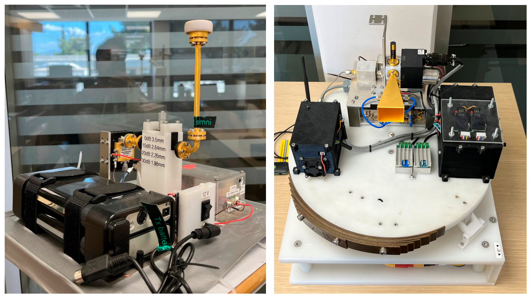
Figure 2.
Top view of the residence building (R4), total distance is 240 meters moving from southwest SW (104m) to northeast NE (136m) of Achilleos street.
Figure 2.
Top view of the residence building (R4), total distance is 240 meters moving from southwest SW (104m) to northeast NE (136m) of Achilleos street.
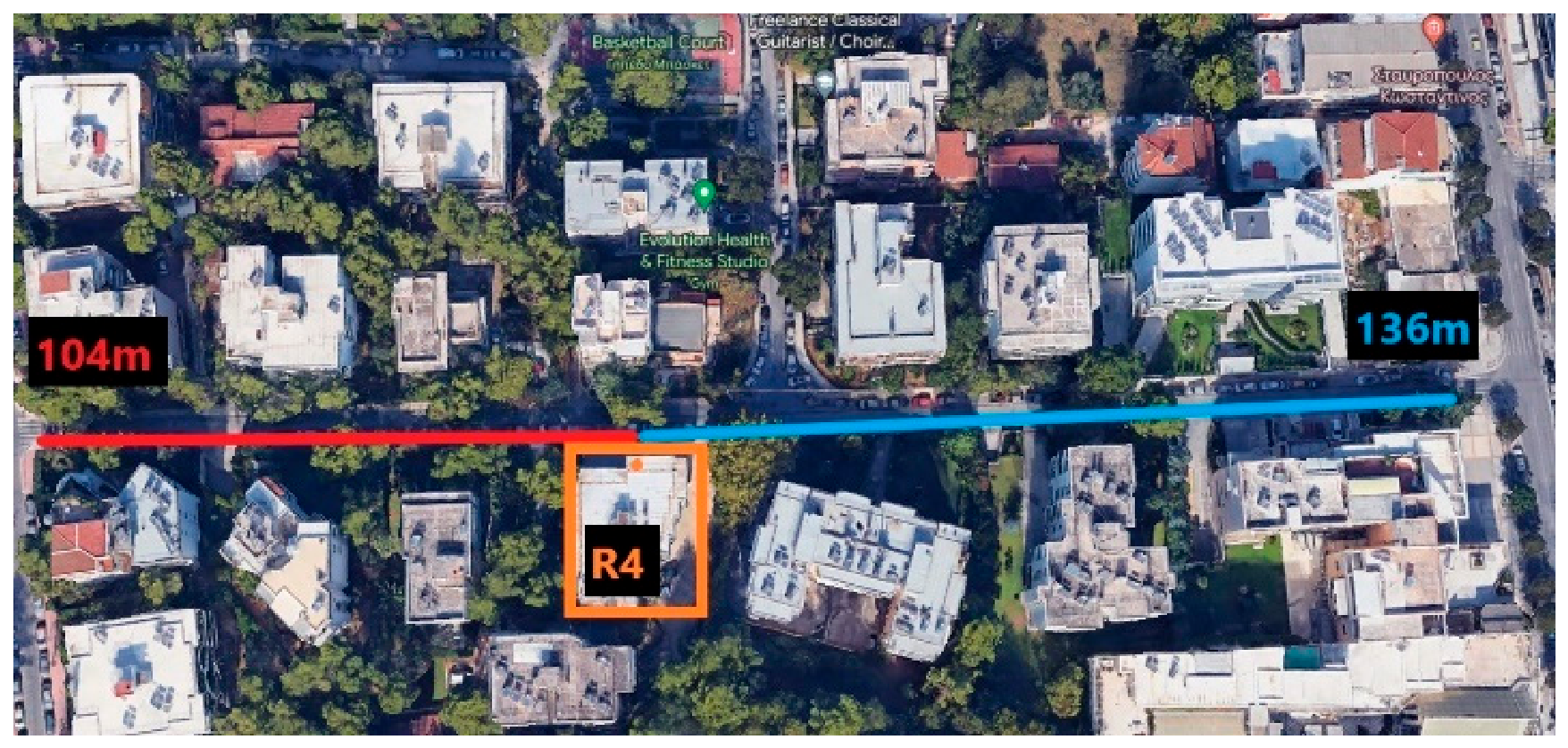
Figure 3.
SW (left) and NE (right) side of Achilleos street facing the residence building R4.
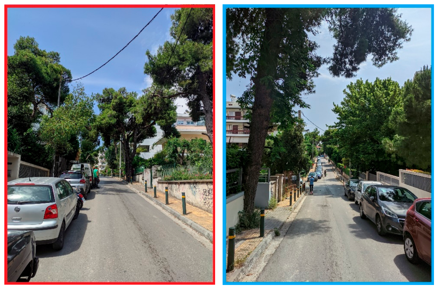
Figure 4.
Top view of the external apartments (EA), the total distance is 326 meters, moving from northeast NE (196m) to southwest SW (130m) of Zefiron street.
Figure 4.
Top view of the external apartments (EA), the total distance is 326 meters, moving from northeast NE (196m) to southwest SW (130m) of Zefiron street.
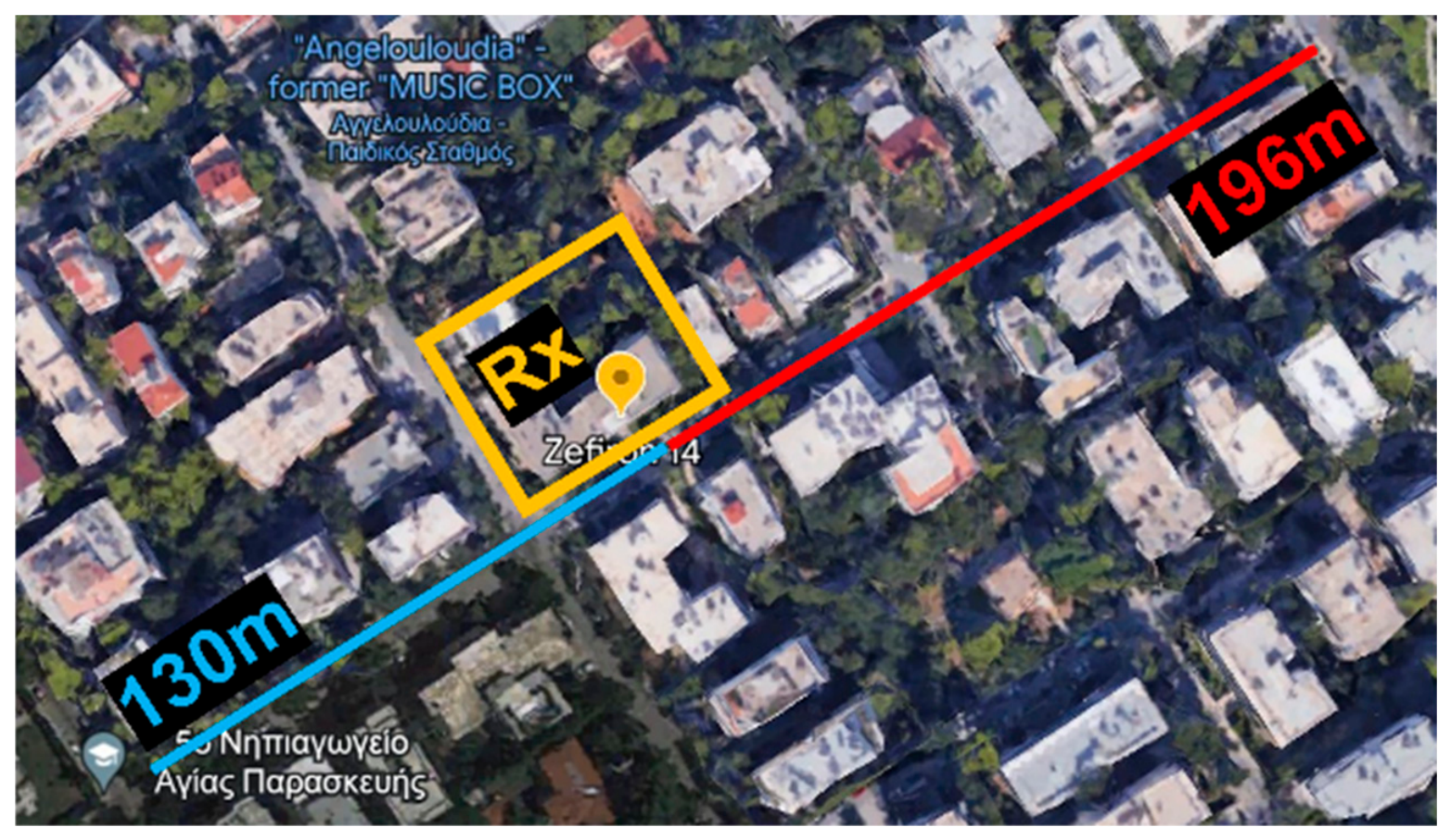
Figure 5.
SW (left photo) and NE (right photo) view of Zefiron Street while looking from the balcony at the 3rd floor at EA site.
Figure 5.
SW (left photo) and NE (right photo) view of Zefiron Street while looking from the balcony at the 3rd floor at EA site.
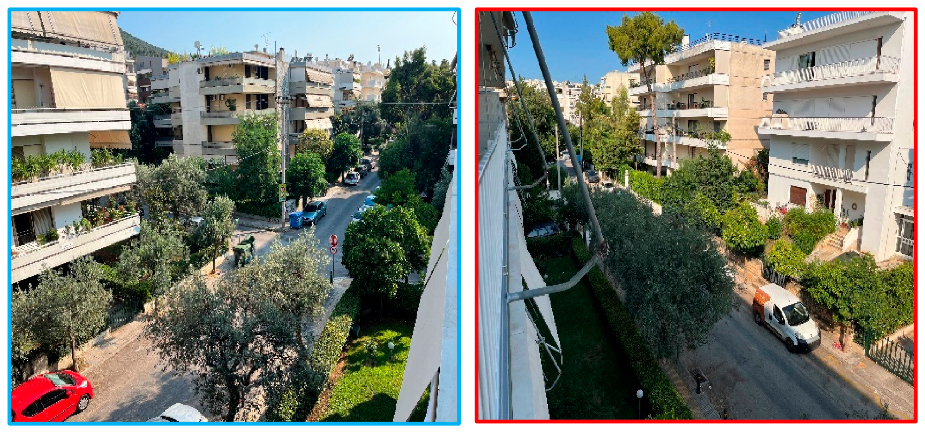
Figure 6.
The balconies in R4 (up) and EA (down) test sites.
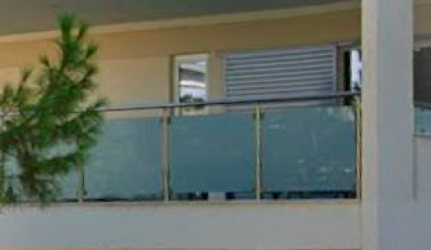
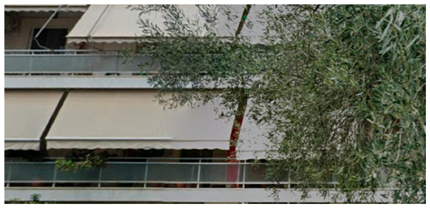
Figure 7.
Top and side view schematics of the measurement set-up depicting all the possible positions of the Rx (balcony and indoors, below and above vegetation) and the Tx of height Zm, as well as the main geometric parameters.
Figure 7.
Top and side view schematics of the measurement set-up depicting all the possible positions of the Rx (balcony and indoors, below and above vegetation) and the Tx of height Zm, as well as the main geometric parameters.
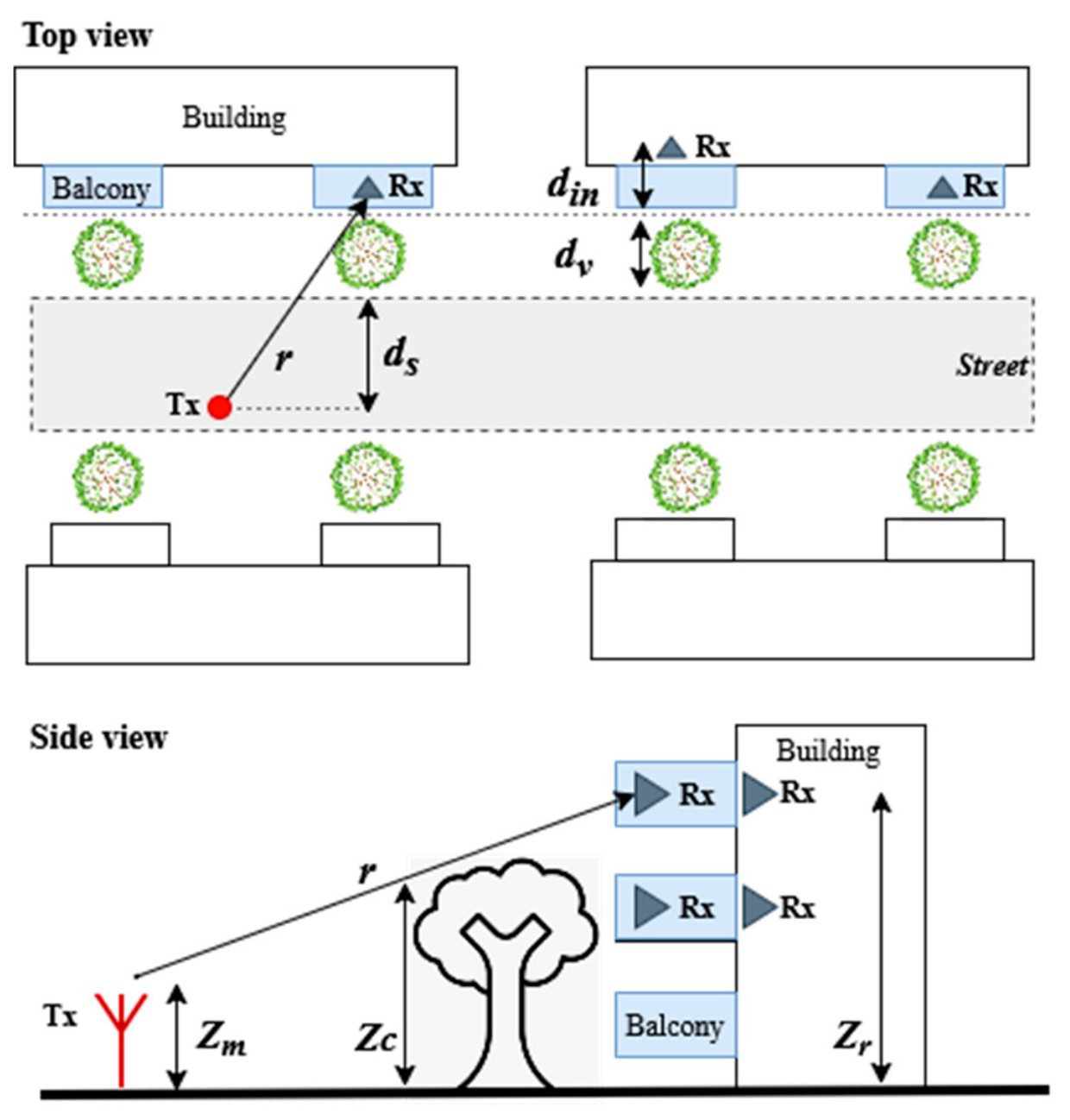
Figure 8.
Path gain versus distance for the NLOS region, outdoor-to-balcony with blue circles and outdoor to indoor with red squares for the two test sites. The lines represent linear least-squares regression fits to the individual datasets.
Figure 8.
Path gain versus distance for the NLOS region, outdoor-to-balcony with blue circles and outdoor to indoor with red squares for the two test sites. The lines represent linear least-squares regression fits to the individual datasets.
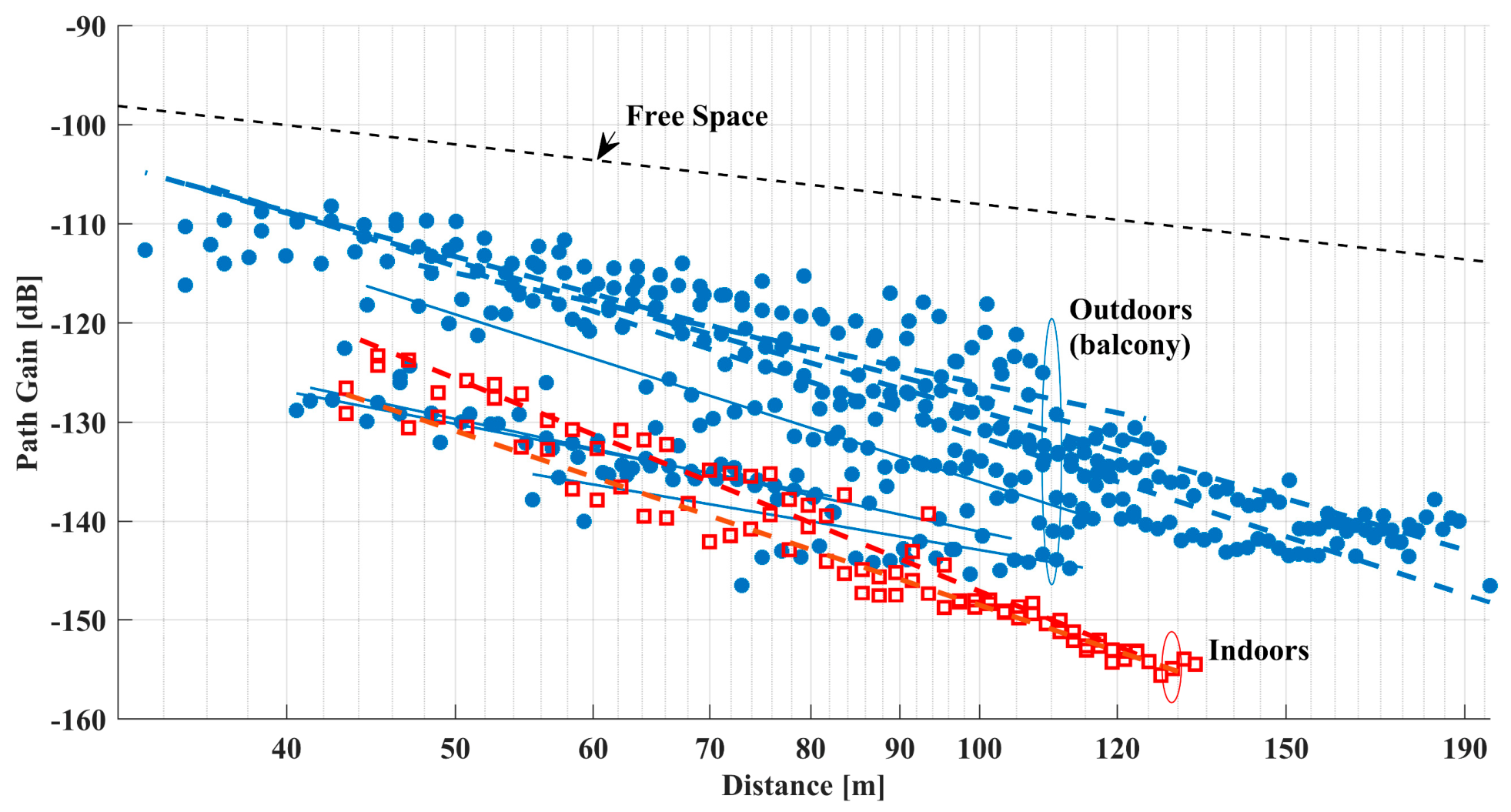
Figure 9.
NLOS path gain for the EA site, 4th floor (above vegetation). Indoor received signals (red boxes) are, on average, 18 dB lower than the corresponding balcony measurements (blue stars).
Figure 9.
NLOS path gain for the EA site, 4th floor (above vegetation). Indoor received signals (red boxes) are, on average, 18 dB lower than the corresponding balcony measurements (blue stars).
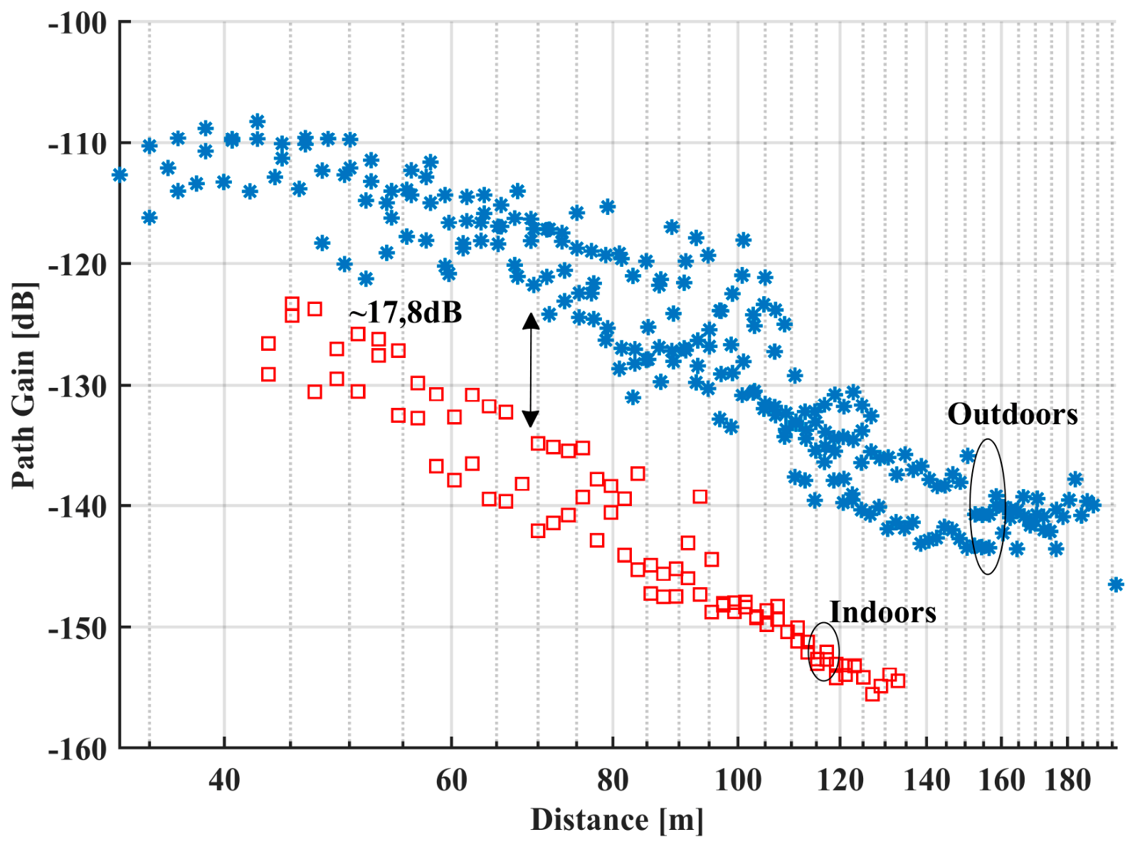
Figure 10.
Measured path gain for O2B links above vegetation (EA site) and the corresponding fits from equations 1, 2b and the 3GPP UMi Street Canyon NLOS model.
Figure 10.
Measured path gain for O2B links above vegetation (EA site) and the corresponding fits from equations 1, 2b and the 3GPP UMi Street Canyon NLOS model.
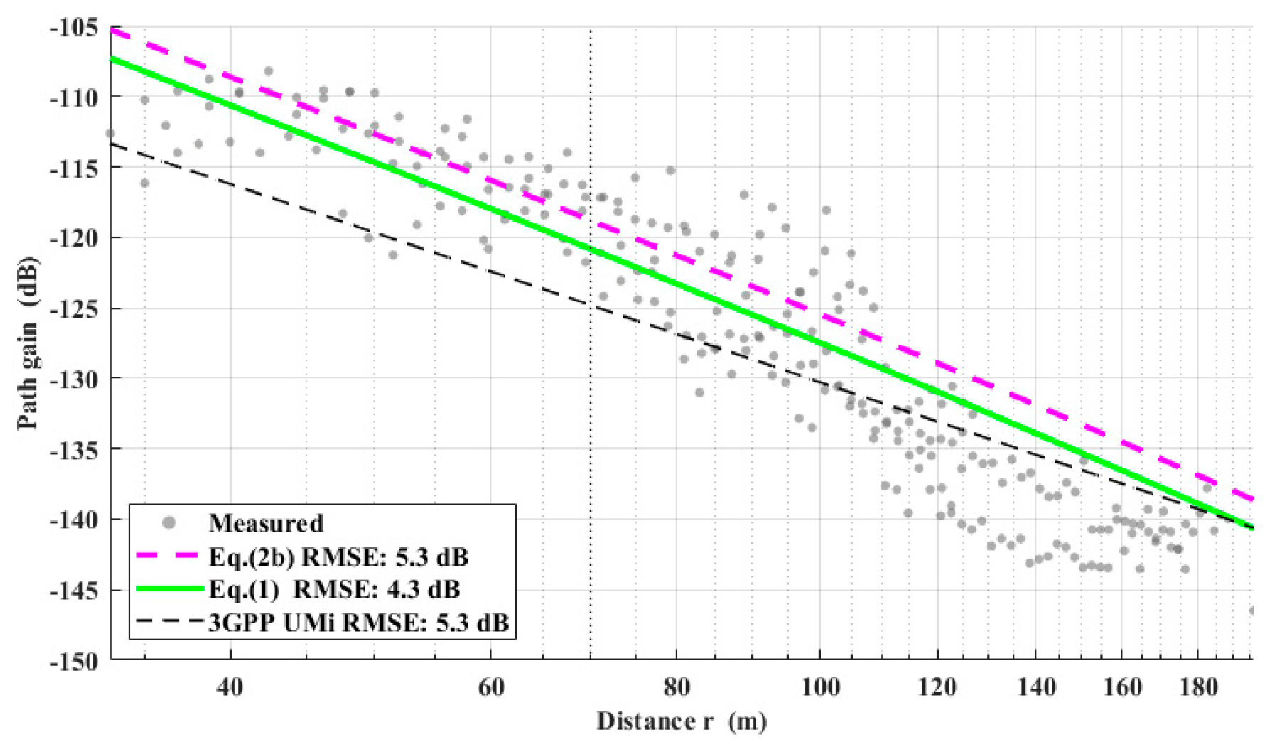
Figure 11.
Measured path gain for O2B links below vegetation (R4 site), and the corresponding fits from eq. 4 and the 3GPP UMi Street Canyon NLOS model.
Figure 11.
Measured path gain for O2B links below vegetation (R4 site), and the corresponding fits from eq. 4 and the 3GPP UMi Street Canyon NLOS model.
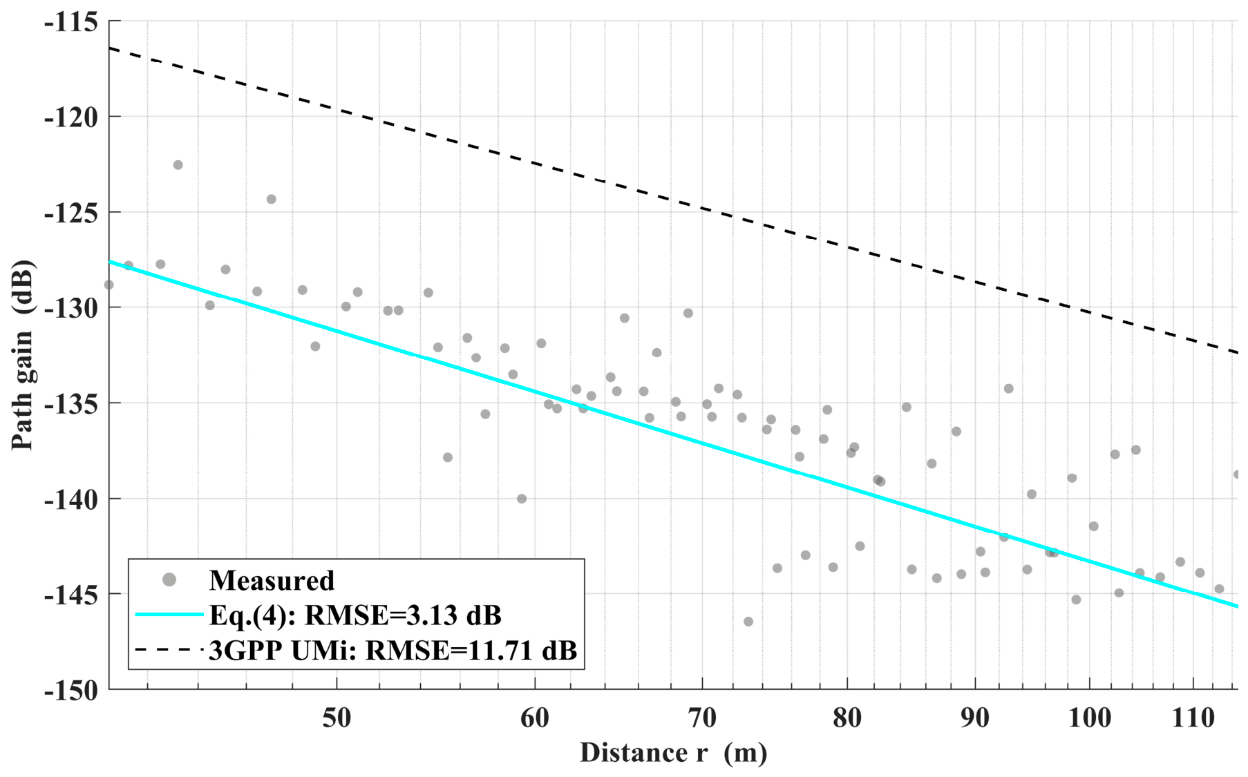
Figure 12.
Measured path gain for O2I links above vegetation (EA site) and the corresponding fits from equations 1, 2b, 3GPP UMi and 3GPP low-loss model.
Figure 12.
Measured path gain for O2I links above vegetation (EA site) and the corresponding fits from equations 1, 2b, 3GPP UMi and 3GPP low-loss model.
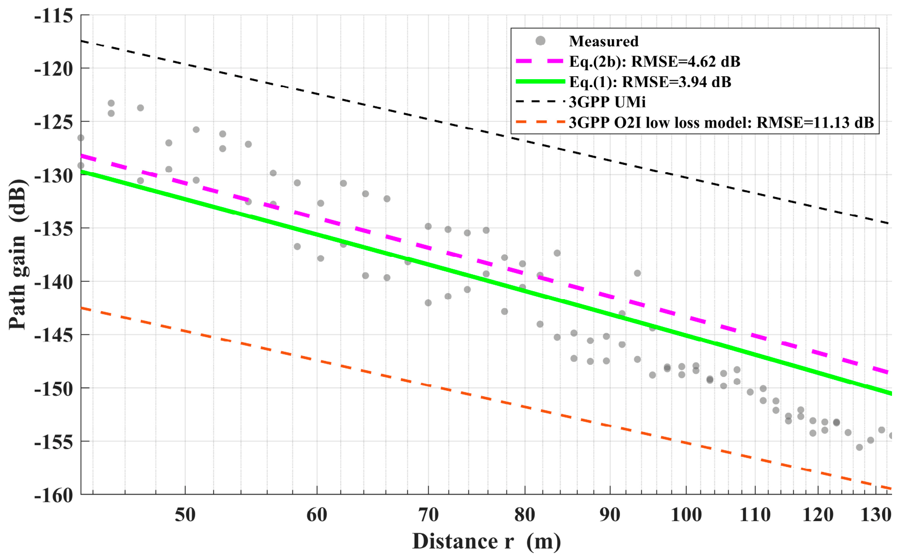
Figure 13.
Measured average PAS (blue solid line) for the EA site, compared with a synthesized ideal Rx-horn reference lobe (red dashed line, HPBW =10∘) aligned with the strongest received direction.
Figure 13.
Measured average PAS (blue solid line) for the EA site, compared with a synthesized ideal Rx-horn reference lobe (red dashed line, HPBW =10∘) aligned with the strongest received direction.
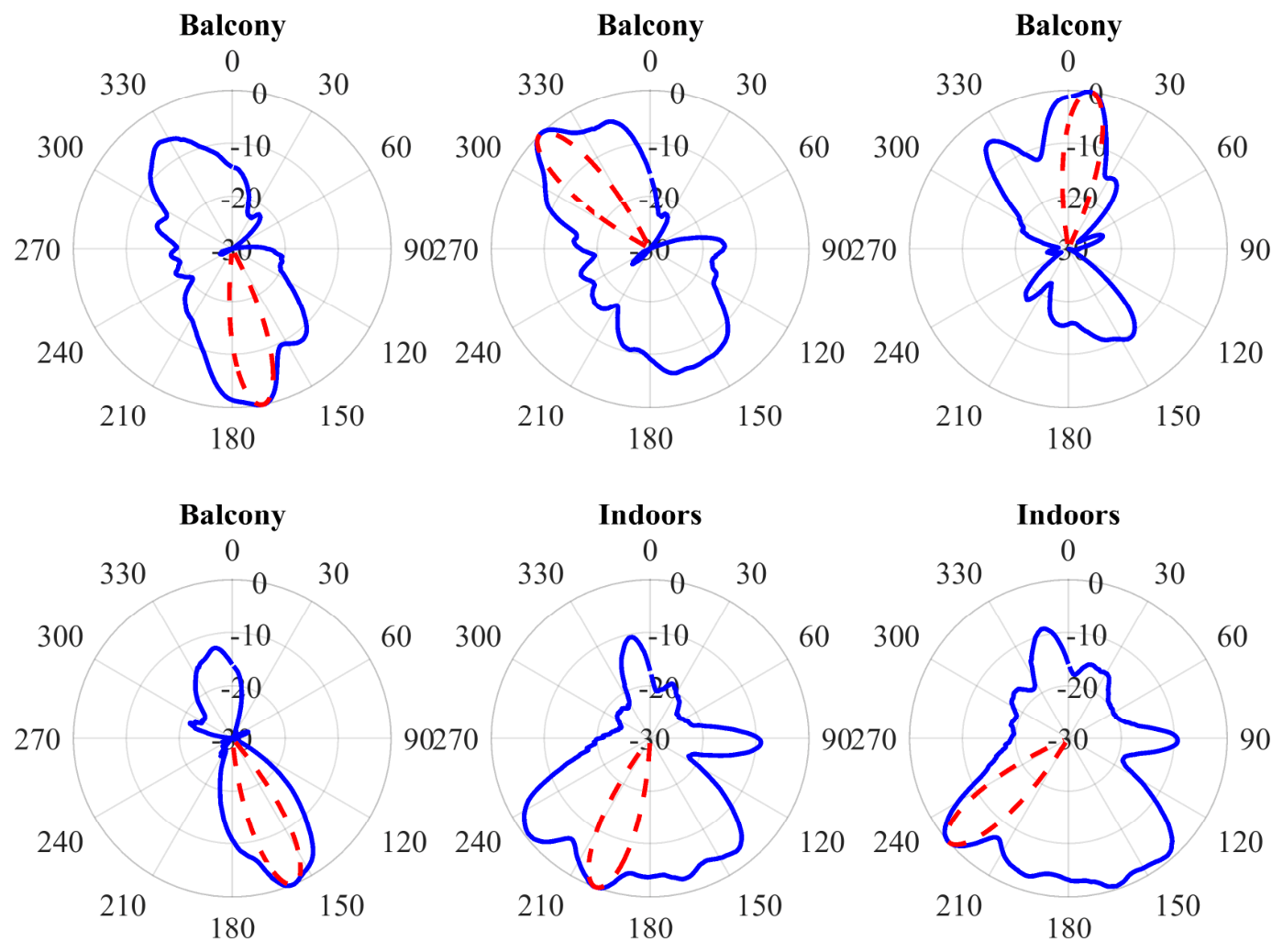
Figure 14.
CDF of the effective measured azimuth gains for LOS and NLOS, indoors and outdoors links in both test sites. Gray regions indicate 90% confidence bands, while the red horizontal line is the 10th percentile. The vertical red line depicts the nominal gain. The blue dotted lines depict the corresponding log-normal fits. The results are comparable to those in [38] and the “Around-the-corner” NLOS case of [39], that used the same or similar spinners and measurement methodology.
Figure 14.
CDF of the effective measured azimuth gains for LOS and NLOS, indoors and outdoors links in both test sites. Gray regions indicate 90% confidence bands, while the red horizontal line is the 10th percentile. The vertical red line depicts the nominal gain. The blue dotted lines depict the corresponding log-normal fits. The results are comparable to those in [38] and the “Around-the-corner” NLOS case of [39], that used the same or similar spinners and measurement methodology.
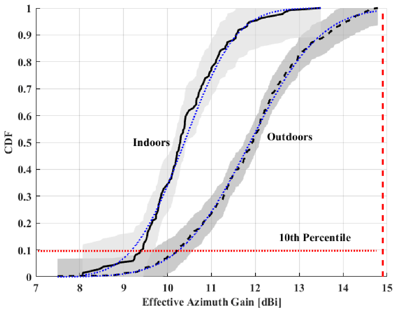
Figure 15.
CDF of the NLOS temporal K-factor along the best (a posteriori) angle for each link. Gray regions indicate 90% confidence bands with the blue dotted lines depicting the corresponding log-normal fits.
Figure 15.
CDF of the NLOS temporal K-factor along the best (a posteriori) angle for each link. Gray regions indicate 90% confidence bands with the blue dotted lines depicting the corresponding log-normal fits.
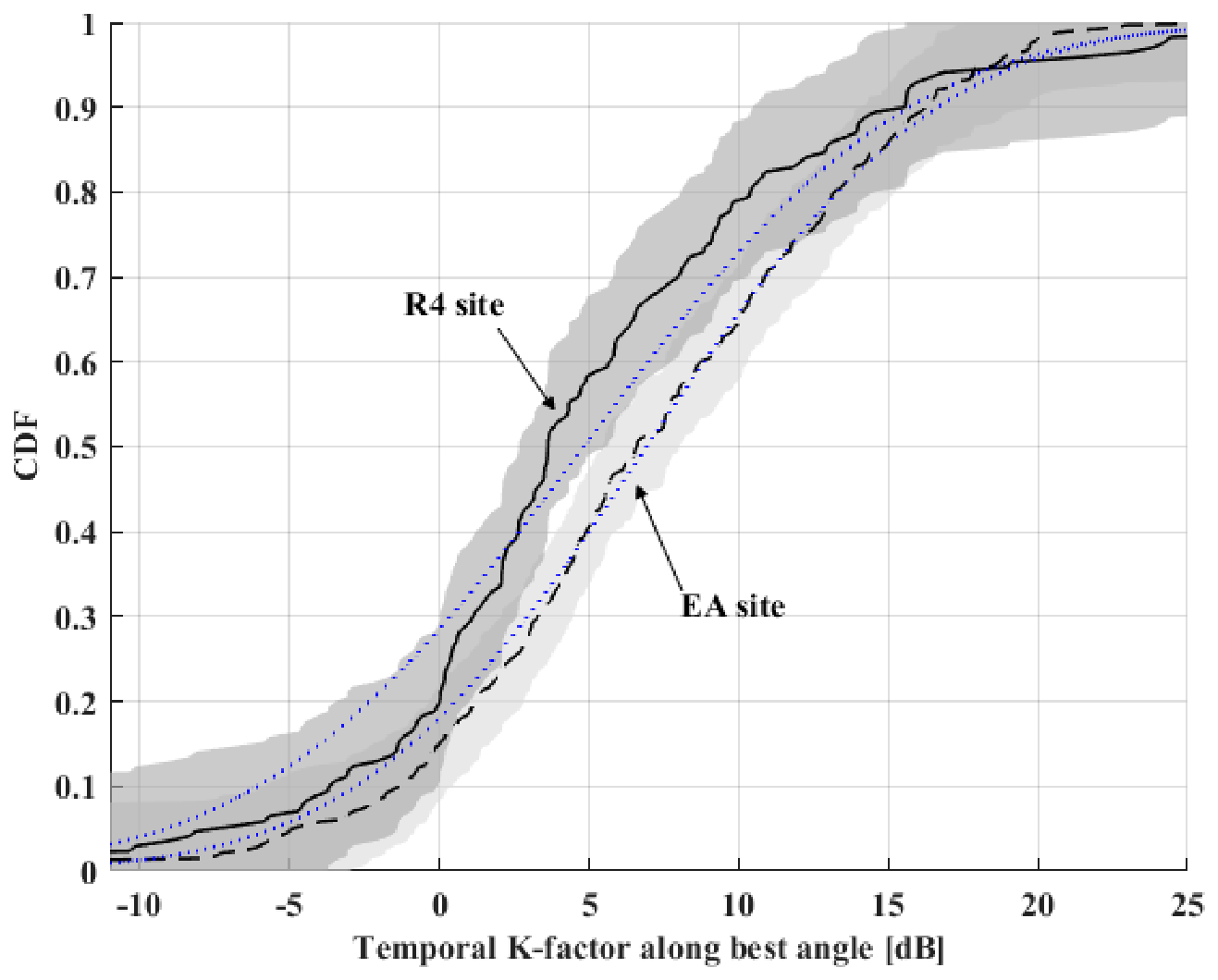
Figure 16.
Top – the received SNR versus distance. Bottom- Estimated 90% downlink Shannon capacity, two path gain models and two receiver-clearance cases at 60 GHz.
Figure 16.
Top – the received SNR versus distance. Bottom- Estimated 90% downlink Shannon capacity, two path gain models and two receiver-clearance cases at 60 GHz.
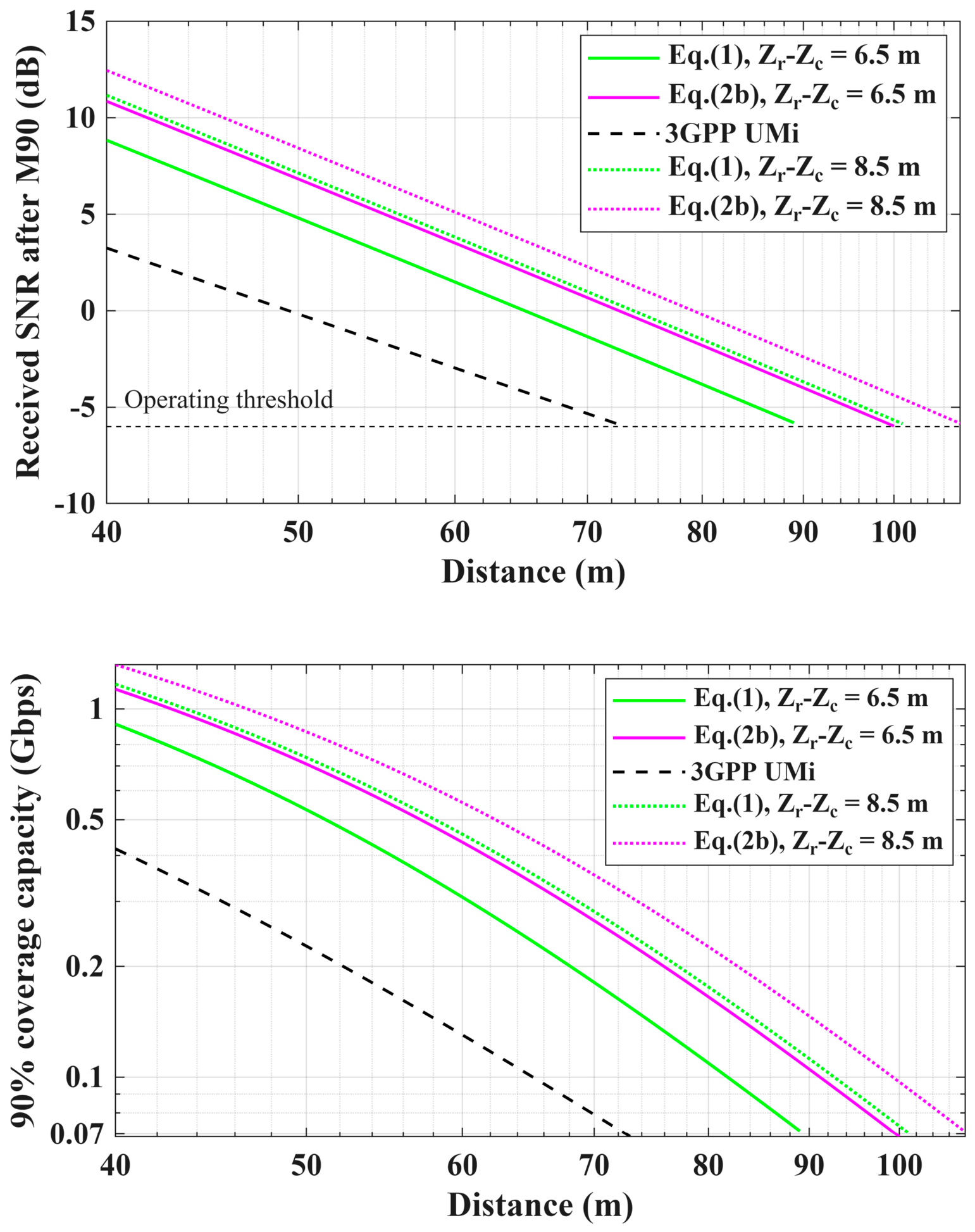

Table 1.
Possible scenarios for channel measurements at two different sites.
| Locations | Level | Proposed Scenarios | |
|---|---|---|---|
| Residence Building-4 | R4 | Level – 1: below vegetation, metalized glass panels on balcony railings and double-glazed metallized glass windows. | Rx on balcony |
| Rx inside | |||
| Level – 4: below vegetation, metalized glass panels on balcony railings and double-glazed metallized glass windows. | Rx on balcony | ||
| Rx inside | |||
| ACG External Apartments | EA-I | Level – 4: above vegetation, plain panels on balcony railings and plain windows. | Rx on balcony |
| Rx inside | |||
| EA-II | Level – 3: above vegetation, plain panels on balcony railings and double-glazed metallized glass windows. | Rx on balcony | |
| Rx inside | |||
Table 2.
Worst-case in-situ window-boundary loss measurement during systems’ calibration showing a 40 dB loss.
Table 2.
Worst-case in-situ window-boundary loss measurement during systems’ calibration showing a 40 dB loss.
| Scenario | Received power (dBm) |
|---|---|
| Calibration without glass | -4.73 |
| Calibration with plain glass window between Tx and Rx | -7.7 |
| Calibration with double-glazed metallized window between Tx and Rx | -44.4 |
Table 3.
Root Mean Square (RMS) errors of path gain models.
| Location | Model parameters | Eq 1 RMS error (dB) | Eq 2b RMS error (dB) |
3GPP RMS error (dB) |
|
|---|---|---|---|---|---|
| O2B for EA-I and EA-II (3rd and 4th floor, above vegetation) |
(average for the two floors) a = 0.0035 Np/m w=10m, , , m, m |
4.3 | 5.3 |
5.3 3GPP UMi |
|
| O2I for EA-I (4th floor, above vegetation, plain glass) |
(Tglass=0.25, Tbalcony=0.82, Tinterior=0.0183) a = 0.0035 Np/m w=10m, , , m, m m m |
4.0 | 4.6 |
15.6 dB 3GPP Umi 11.13 3GPP low loss model |
|
| Location | Model parameters |
Eq 4 RMS error (dB) |
3GPP UMi RMS error (dB) | ||
| O2B for R4 (below vegetation) |
W=10.5 m a = 0.0035 Np/m |
3.13 | 11.71 | ||
Disclaimer/Publisher’s Note: The statements, opinions and data contained in all publications are solely those of the individual author(s) and contributor(s) and not of MDPI and/or the editor(s). MDPI and/or the editor(s) disclaim responsibility for any injury to people or property resulting from any ideas, methods, instructions or products referred to in the content. |
© 2026 by the authors. Licensee MDPI, Basel, Switzerland. This article is an open access article distributed under the terms and conditions of the Creative Commons Attribution (CC BY) license (http://creativecommons.org/licenses/by/4.0/).
Copyright: This open access article is published under a Creative Commons CC BY 4.0 license, which permit the free download, distribution, and reuse, provided that the author and preprint are cited in any reuse.