Prediction of the Higgs Mass from a Quantum Field Theory with a Specific Lorentz-Violating Model

2. Review of the Kinematically Modified Lorentz Model

Lorentz violation is a central subject in modern fundamental physics. Among the Lorentz-violating models in the literature, doubly special relativity (DSR) is one of the most renowned and extensively studied frameworks. Beyond the speed of light, DSR postulates an additional frame-independent constant, either a maximum energy or a minimum length, which modifies the particle dispersion relation as $E^2=p^2+m^2+\eta L_p^{\alpha }{p}^2{E}^{\alpha }+o(L_p^{\alpha +1}{E}^{\alpha +3})$, where L_p denotes the “Planck length”, α is a positive integer and η is a real number [3,4]. However, the DSR framework suffers from non-trivial complexity, as it involves numerous undetermined parameters whose physical interpretations remain ambiguous [5]. To address this issue, a novel Lorentz-violating model was proposed in Ref. [6,7]. This model possesses a mathematical structure highly analogous to the conventional Lorentz framework and introduces only a single free parameter in the modified particle dispersion relation. A prominent feature of this model is that it naturally recovers standard Lorentz symmetry at low and intermediate energy scales. In contrast, for particles moving at velocities approaching the speed of light c, the total energy converges to a finite value rather than diverging to infinity as predicted by standard Lorentz relativity. Although this finite-energy behavior is qualitatively reminiscent of DSR, the two mechanisms differ fundamentally: the energy bound in Ref. [6,7] is mass-dependent and varies with the particle rest mass, whereas the DSR energy limit corresponds to the Planck energy and is entirely mass-independent. For completeness and to clarify the theoretical foundation of the present work, we briefly review the Lorentz-violating model of Ref. [6,7] in the following section.

The constancy of the local speed of light serves as the core postulate of relativity. Accordingly, most Lorentz-violating models admit a variable local speed of light, which naturally modifies the dispersion relations of massive particles. In Ref. [6,7], a fundamental hypothesis concerning the correlation between the speed of light and the motion of the light source was proposed. Specifically, the speed of light measured by an observer moving with velocity v relative to the light source is assumed to be nc, where n denotes a dimensionless parameter. To comply with low- and intermediate-energy experimental observations of both special and general relativity, the parameter n must satisfy rigorous symmetry constraints: n(v,c)= n(-v,c)= n(v,-c)= n(-v,-c) and n(v=0, c)=1. The physical justification for these constraints is provided in full detail in Ref. [6]. Based on the above hypothesis, the corresponding analytical equations can be formulated as follows.

$$\left\{\begin{array}{l}{x}^2+y^2+z^2={(ct)}^2\\ x^{\prime 2}+y^{\prime 2}+z^{\prime 2}={({nct}^{\prime })}^2\\ y=y^{\prime }=0\\ z=z^{\prime }=0\end{array}\right.\mathrm{or}\left\{\begin{array}{l}{x}^{\prime 2}+y^{\prime 2}+z^{\prime 2}={({ct}^{\prime })}^2\\ x^2+y^2+z^2={(nct)}^2\\ y=y^{\prime }=0\\ z=z^{\prime }=0\end{array}\right.$$

(1)

Here, (x, y, z, t) denotes the coordinates of inertial frame S, and (x’, y’, z’, t’) corresponds to inertial frame S’. For simplicity, the spatial axes of the two frames are taken to be mutually parallel, with the relative velocity v aligned along the x- and x’-axes.

The first relation in Eq. (1) describes the scenario where the light source is at rest in frame S. In this case, an observer stationary in S measures a light speed as c, consistent with the constraint n(v=0, c)=1, while an observer in frame S’ measures a light speed as nc. By symmetry, frames S and S’ are equivalent. If the light source is instead fixed in S’, an observer in S’ measures c, whereas an observer in S obtains nc. This behavior is encoded in the second relation of Eq. (1).

From Eq. (1), one can obtain the following coordinate transformation between two inertial frames in relative motion with velocity v:

$$\left\{\begin{array}{l}{\mathit{x}}^{\prime }=\gamma (\mathit{x}-\mathit{v}t)\\ t^{\prime }=\gamma (t-{\displaystyle \frac{\mathit{v}}{k^2(\mathit{v},\mathit{c})}}x)\end{array}\right.$$

(2)

where $\gamma (\mathit{v},\mathit{c})=1/\sqrt{1-{\mathit{v}}^2/k^2}$, $k(\mathit{v},\mathit{c})=\sqrt{n\mathit{v}{\mathit{c}}^2/(n\mathit{c}-\mathit{c}+\mathit{v})}$. Note that n satisfies the condition that n(v,c)= n(-v,c)=n(v,-c)=n(-v,-c) and n(v=0, c)=1.

To further clarify the physical meaning of Eq. (2), we conversely deduce the relation between the light source and the speed of light from it. This yields the following

$${\displaystyle \frac{d{\mathit{x}}^{\prime }}{d{t}^{\prime }}}={\displaystyle \frac{\mathit{d}x-\mathit{v}dt}{dt-\frac{\mathit{v}}{k^2(\mathit{v},\mathit{c})}d\mathit{x}}}={\displaystyle \frac{d\mathit{x}/dt-\mathit{v}}{1-\frac{\mathit{v}}{k^2(\mathit{v},\mathit{c})}\frac{d\mathit{x}}{dt}}}=f(\mathit{v},\mathit{c})$$

(3)

Since v and c are both vectors, they admit four possible sign combinations, namely (v, c), (v, -c), (-v, c) and (-v, -c). Based on Eq. (3), we then obtain the following cases.

Case 1: When the light source is at rest in frame S, an observer in S measures the speed of light as c, whereas an observer in S’ measures it as

$$\left\{\begin{array}{l}when{\displaystyle \frac{dx}{dt}}=c,{\displaystyle \frac{{\mathit{dx}}^{\prime }}{{\mathit{dx}}^{\prime }}}=f(v,c)={\displaystyle \frac{c-v}{1-\frac{v}{k^2(v,c)}c}}=f(-v,c)={\displaystyle \frac{c+v}{1-\frac{-v}{k^2(-v,c)}c}}=nc\\ when{\displaystyle \frac{dx}{dt}}=-c,{\displaystyle \frac{{\mathit{dx}}^{\prime }}{{\mathit{dx}}^{\prime }}}=f(v,-c)={\displaystyle \frac{-c-v}{1-\frac{v}{k^2(v,-c)}(-c)}}=f(-v,-c)={\displaystyle \frac{-c+v}{1-\frac{-v}{k^2(-v,-c)}(-c)}}=-nc\end{array}\right.$$

(4)

Case2: Similarly, since frames S and S’ are equivalent, if the light source is at rest in S’, an observer in S’ measures the speed of light as c, while an observer in S measures it as (in this case the velocity of S relative to the light source is -v)

$$\left\{\begin{array}{l}{\displaystyle \frac{dx}{dt}}={\displaystyle \frac{d{x}^{\prime }/d{t}^{\prime }-(-\mathit{v})}{1-\frac{-\mathit{v}}{k^2(-\mathit{v},\mathit{c})}\frac{d{x}^{\prime }}{d{t}^{\prime }}}}=f^{\prime }(\mathit{v},\mathit{c})\\ when {\displaystyle \frac{d{x}^{\prime }}{d{t}^{\prime }}}=c,{\displaystyle \frac{\mathit{dx}}{\mathit{dt}}}=f^{\prime }(v,c)={\displaystyle \frac{c+v}{1+\frac{v}{k^2(-v,c)}c}}=f^{\prime }(-v,c)={\displaystyle \frac{c-v}{1-\frac{v}{k^2(v,c)}c}}=nc\\ when {\displaystyle \frac{d{x}^{\prime }}{d{t}^{\prime }}}=-c,{\displaystyle \frac{\mathit{dx}}{\mathit{dt}}}=f^{\prime }(v,-c)={\displaystyle \frac{-c+v}{1+\frac{v}{k^2(-v,-c)}(-c)}}=f^{\prime }(-v,-c)={\displaystyle \frac{-c-v}{1+\frac{-v}{k^2(v,-c)}(-c)}}=-nc\end{array}\right.$$

(5)

Combining Eqs. (4) and (5), one obtains the following vector expression:

$$\left\{\begin{array}{l}when {\displaystyle \frac{d\mathit{x}}{dt}}=\mathit{c},{\displaystyle \frac{{d\mathit{x}}^{\prime }}{{\mathit{dx}}^{\prime }}}=n\mathit{c}\\ when {\displaystyle \frac{{d\mathit{x}}^{\prime }}{{dt}^{\prime }}}=\mathit{c},{\displaystyle \frac{d\mathit{x}}{\mathit{dt}}}=n\mathit{c}\end{array}\right.$$

(6)

Eq. (6) is an alternative form of Eq. (1) and encodes the same physical content. One can see that the coordinate transformation obtained in Eq. (2) is mathematically highly analogous to the Lorentz transformation. In fact, replacing c by k in the Lorentz transformation yields Eq. (2) directly. Owing to this similarity, it can be readily shown that Maxwell’s equations remain covariant under Eq. (2). Furthermore, it is quite obvious that for Eq. (2), the corresponding dispersion relation of particles is

$$E^2={\mathit{p}}^2{k}^2+E_0^2$$

(7)

where E=γm₀k² denotes the total energy of particles, E₀=m₀k², p=γm₀v denotes the momentum of particles, and here m₀ denotes the rest mass of particles.

A key question then arises, namely, what is the explicit form of n in Eq. (2)? Obviously, when n≡1, all the above results reduce to the Lorentz case. However, the author of Ref. [6] noted that the following choice of n renders both the spacetime scaling factor γ and the total energy E of particles finite, rather than divergent as predicted by the Lorentz model, that is

$$n(v)={\displaystyle \frac{1}{1-Q}}(1-Q^{1-v^2/c^2})$$

(8)

$$\underset{\mathit{v}\to \mathit{c}}{\mathbf{lim}}\gamma =\underset{\mathit{v}\to \mathit{c}}{\mathbf{lim}}{\displaystyle \frac{1}{\sqrt{1-{\mathit{v}}^2/k^2}}}=\underset{v\to c}{\mathbf{lim}}{\displaystyle \frac{1}{\sqrt{(\frac{1-\mathit{v}/\mathit{c}}{n})(n+\frac{\mathit{v}}{\mathit{c}})}}}=\sqrt{{\displaystyle \frac{2\mathbf{ln}Q}{Q-1}}}$$

(9)

$$\underset{\mathit{v}\to \mathit{c}}{\lim }E=\underset{\mathit{v}\to \mathit{c}}{\lim }\gamma m_0{k}^2=E_{QG}={\displaystyle \frac{m_0{\mathit{c}}^2}{[1-0.5(Q-1)/\ln Q]}}\sqrt{{\displaystyle \frac{2\ln Q}{Q-1}}}$$

(10)

$$\underset{\mathit{v}\to \mathit{c}}{\lim }p=\underset{\mathit{v}\to \mathit{c}}{\lim }\gamma m_{0}v=m_0\mathit{c}\sqrt{{\displaystyle \frac{2\ln Q}{Q-1}}}=\xi m_0$$

(11)

where Q is a constant.

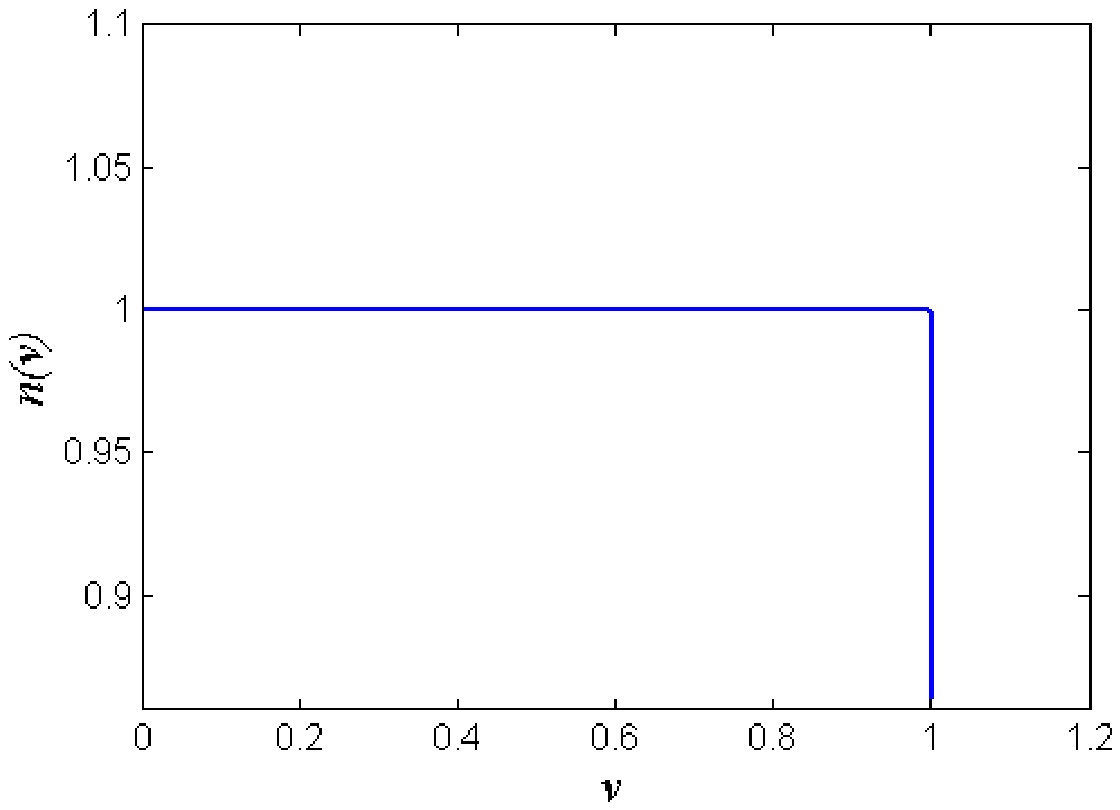
Figure 1 displays the curve of n(v). From Figure 1 we can see that, over a wide range of v, n remains extremely close to 1. This property ensures that Eq. (2) closely approximates the Lorentz transformation at low and intermediate energies and hence does not conflict with the extensive experimental results obtained at these scales. In other words, since extensive low- and intermediate-energy experiments show no significant deviations from the predictions of the Lorentz model, one can conclude that Q ≃0. Furthermore, the smaller the value of Q, the higher the energy at which Eq. (2) deviates significantly from the Lorentz model. In the limit Q=0, all the above equations reduce to their Lorentz-model counterparts.

In the preceding discussion, we have reviewed the special Lorentz-violating model proposed in Ref. [6]. This model possesses two major advantages over DSR. First, it is more economical, as it involves only a single undetermined parameter. Second, the energy limit of a particle is encoded in the general coordinate transformation of Eq. (2), rather than being introduced as an additional assumption as in the DSR framework. Furthermore, there is another significant difference. In the present model, the energy limit of a particle, as given in Eq. (10), depends on its rest mass. In the DSR framework, by contrast, the energy limit is assumed to be a mass-independent constant. As will be shown below, this difference provides a possible resolution of the hierarchy problem in the Standard Model.

Now let’s analyze the dispersion relation of particles. When v approaches c, there is

$$\underset{v\to c}{\lim }{k}^2=\underset{v\to c}{\lim }{\displaystyle \frac{nv{c}^2}{nc-c+v}}={\displaystyle \frac{2\ln Q}{2\ln Q-Q+1}}$$

(12)

Since Q ≃0, it follows that k² approaches 1 very closely as v approaches c. And we have already established that k = 1 when v = 0. This implies that k remains extremely close to 1 over the entire range v ∈ [0, c]. Consequently, the dispersion relation of the particles in this work may be approximated as identical to that of the Lorentz model, except that the energy or momentum range is no longer unbounded. Therefor, in the subsequent analysis, we treat the energy–momentum dispersion relation of the particles (i.e., Eq. (7)) as still approximately that of the Lorentz model, with the sole modification that the particle energy and momentum are cut off by Eqs. (10) and (11).

3. The Scale-Invariant Standard Model and the One-Loop Effective Potential

3.1. The Scale-Invariant Tree-Level Potential

In the unitary gauge, the tree-level Higgs potential for the background field φ is given by

$$V_{tree}(\varphi )={\displaystyle \frac{\lambda }{4}}{\varphi }^4$$

(13)

We assume that the present model possesses exact classical scale invariance at the cutoff scale, namely, the absence of any bare mass term. This assumption is an independent postulate of the present work. Although its form resembles the flatness condition in the asymptotically safe gravity framework, the physical origin is different. There, the flatness condition arises from the gravitational fixed point [8,9]. Here, it is imposed so that the advantage of the mass-dependent cutoff can be fully exploited, and all masses are generated dynamically by radiative corrections. Therefor, the tree-level squared masses of particles in the background field are given by

$$m_{0t}^2(\varphi )={\displaystyle \frac{y_t^2}{2}}{\varphi }^2,m_{0W}^2(\varphi )={\displaystyle \frac{g^2}{4}}{\varphi }^2,m_{0Z}^2(\varphi )={\displaystyle \frac{g^2+g^{\prime 2}}{4}}{\varphi }^2,m_{0h}^2(\varphi )=3\lambda {\varphi }^2$$

(14)

3.2. The One-Loop Effective Potential

In Euclidean space, the one-loop contribution to the effective potential reads

$$\Delta V_i=\pm {\displaystyle \frac{g_i}{32{\pi }^2}}{\displaystyle {\int }_0^{{\Lambda }_i^2}u\ln (1+\frac{m_{0i}^2}{u})du}$$

(15)

where Λ_i=ξm_0i, and the factor 1/(32π²) originates from the following path integral measure

$${\displaystyle \int \frac{d^4{k}_E}{{(2\pi )}^4}=\frac{1}{16{\pi }^2}{\displaystyle {\int }_0^{{\Lambda }^2}udu}}$$

(16)

Together with the factor 1/2, this yields 1/(32π²).

For later use, here we define the following integral

$$I(a,\Lambda )\equiv {\displaystyle {\int }_0^{{\Lambda }^2}u\ln (1+\frac{a}{u})}du$$

(17)

Integrating by parts, one obtains

$$I(a,\Lambda )={\displaystyle \frac{{\Lambda }^4}{2}}\ln (1+{\displaystyle \frac{a}{{\Lambda }^2}})+{\displaystyle \frac{a{\Lambda }^2}{2}}-{\displaystyle \frac{a^2}{2}}\ln (1+{\displaystyle \frac{{\Lambda }^2}{a}})$$

(18)

Expanding ln(1+a/Λ²) and using Λ²=ξ²a, one obtains

$$I(a,\Lambda )=a^2({\xi }^2-\ln \xi -{\displaystyle \frac{1}{4}})+o({\displaystyle \frac{a^3}{{\Lambda }^2}})$$

(19)

Let us define

$$K={\xi }^2-\ln \xi -{\displaystyle \frac{1}{4}}$$

(20)

Then up to order a², we obtain

$$I(m_{0i}^2,{\Lambda }_i)=m_{0i}^{4}K$$

(21)

Note that, in this expression, Λ_i=ξm_0i already carries the dependence on the field φ. When the derivatives with respect to φ are subsequently taken, the boundary-term contributions are automatically incorporated into the derivatives of m_0i⁴K with respect to φ. Appendix A provides a rigorous verification of this point.

For each particle species, the contribution is given by

(1)

For the top quark, a fermion with 12 degrees of freedom, the contribution enters with a minus sign and is given by

$$V_t=-{\displaystyle \frac{12}{32{\pi }^2}}{m}_{0t}^{4}K=-{\displaystyle \frac{3y_t^4}{32{\pi }^2}}{\varphi }^{4}K$$

(22)

(2)

For the W boson, which has 3 degrees of freedom, the contribution enters with a plus sign and is given by

$$V_W={\displaystyle \frac{3}{32{\pi }^2}}{m}_{0W}^{4}K={\displaystyle \frac{3g^4}{512{\pi }^2}}{\varphi }^{4}K$$

(23)

(3)

For the Z boson, which has 3 degrees of freedom, the contribution enters with a plus sign and is given by

$$V_Z={\displaystyle \frac{3{(g^2+g^{\prime 2})}^2}{512{\pi }^2}}{\varphi }^{4}K$$

(24)

(4)

For the Higgs boson, which has 1 degree of freedom, the contribution enters with a plus sign and is given by

$$V_h={\displaystyle \frac{1}{32{\pi }^2}}{m}_{0h}^{4}K={\displaystyle \frac{9{\lambda }^2}{32{\pi }^2}}{\varphi }^{4}K$$

(25)

Combining the above contributions, the total effective potential reads

$$V_{eff}(\varphi )={\displaystyle \frac{{\varphi }^4}{4}}[\lambda +(-{\displaystyle \frac{3y_t^4}{8{\pi }^2}}+{\displaystyle \frac{3g^4}{128{\pi }^2}}+{\displaystyle \frac{3{(g^2+g^{\prime 2})}^2}{128{\pi }^2}}+{\displaystyle \frac{9{\lambda }^2}{8{\pi }^2}})K]$$

(26)

From Eq. (26) it can be seen that, the large term generated by the hard cutoff is a φ⁴ term rather than a φ² term, and therefor does not contribute to the squared Higgs mass. The mass squared can only arise from the logarithmic terms or from the renormalization group evolution. Next, we will see that this fact lies at the heart of the resolution of the hierarchy problem.

4. RG Improvement and Electroweak Symmetry Breaking

4.1. Complete Two-Loop RG Equations

In our numerical calculations, we employ the complete two-loop renormalization group equations of the Standard Model. The coefficients are taken from the classic paper by Machacek and Vaughn [10]. The one-loop part is given by

$$\begin{array}{l}16{\pi }^2{\beta }_{g_3}^{(1)}=-7g_3^3,16{\pi }^2{\beta }_g^{(1)}=-{\displaystyle \frac{19}{6}}{g}^3,16{\pi }^2{\beta }_{g^{\prime }}^{(1)}={\displaystyle \frac{41}{6}}{g}^{\prime 3},\\ 16{\pi }^2{\beta }_{yt}^{(1)}=y_t({\displaystyle \frac{9}{2}}{y}_t^2-8g_3^2-{\displaystyle \frac{9}{4}}{g}^2-{\displaystyle \frac{17}{12}}{g}^{\prime 2}),\\ 16{\pi }^2{\beta }_{\lambda }^{(1)}=24{\lambda }^2+12\lambda y_t^2-6y_t^4+{\displaystyle \frac{3}{8}}[2g^4+{(g^2+g^{\prime 2})}^2]\end{array}$$

(27)

The two-loop part β_i⁽²⁾ contains a large number of terms, such as g₃⁵, g₃²y_t³, y_t⁵ and λy_t⁴. The complete expressions are given in Ref. [10]. In our numerical solution, we employ these full expressions without any truncation or approximation.

4.2. Boundary Conditions and the Self-Consistent Cutoff Scale

Here we introduce an additional independent assumption, namely, that the scale-invariant flatness condition is satisfied at the ultraviolet scale μ₀

$$\lambda ({\mu }_0)=0,{\beta }_{\lambda }({\mu }_0)=0$$

(28)

where μ₀ is determined self-consistently by the following intrinsic cutoff

$${\mu }_0=\xi m_t({\mu }_0)=\xi {\displaystyle \frac{y_t({\mu }_0)v}{\sqrt{2}}}$$

(29)

This condition takes the same form as the flatness condition in the asymptotically safe gravity framework. However, μ₀ is not the fixed Planck scale. Instead, it is determined dynamically by the particle masses. Physically, this reflects the requirement that, at the kinematic cutoff scale, the theory contain no mass parameter.

4.3. Numerical Solution Strategy and Pole Mass Conversion

For the low-energy inputs, we adopt the PDG 2024 recommended values [11]: M_Z=91.1876 GeV, G_F=1.1663787×10^-5 GeV^-2, α_s(M_Z)=0.1180, M_t^pole=172.5 GeV, M_h^pole=125.1 GeV. The electroweak scale is defined through the Fermi constant G_F as

$$v={(\sqrt{2}{G}_F)}^{-1/2}=246.21965\mathrm{GeV}$$

(30)

In the $\stackrel{\_\_\_\_}{\mathrm{MS}}$ scheme, the gauge couplings evaluated at M_Z read

$$g(M_Z)=0.65194,g^{\prime }(M_Z)=0.35761,g_3(M_Z)=\sqrt{4\pi {\alpha }_s(M_Z)}=1.220$$

(31)

The shooting parameters are taken to be

$$\mathbf{x}=(y_t(M_z),\xi ,\lambda (M_Z))$$

(32)

The objective function is defined as

$$\begin{array}{l}{F}_1=\lambda ({\mu }_0)\\ F_2={\beta }_{\lambda }({\mu }_0)\\ F_3=M_t^{\mathrm{calc}}-172.5\mathrm{GeV}\\ F_4=M_h^{\mathrm{calc}}-125.1\mathrm{GeV}\end{array}$$

(33)

The numerical procedure consists of the following steps, with the complete two-loop beta functions used at each step:

Step 1: Initialization. We assign trial values to y_t(M_Z), ξ and λ(M_Z).

Step 2: Determine the ultraviolet scale μ₀. Using μ₀=ξm_t(μ₀) together with m_t(μ)=y_t(μ)v/sqrt(2), one solves for μ₀ by the following fixed-point iteration

$${\mu }_0^{(n+1)}=\xi {\displaystyle \frac{y_t({\mu }_0^{(n)})v}{\sqrt{2}}}$$

(34)

Here, y_t(μ₀⁽ⁿ⁾) is obtained by integrating the couplings from M_Z up to μ₀⁽ⁿ⁾. The initial estimate is taken as μ₀⁽⁰⁾=ξy_t(M_Z)v/sqrt(2). The iteration proceeds until the convergence criterion |μ₀⁽ⁿ⁺¹⁾-μ₀⁽ⁿ⁾|/μ₀⁽ⁿ⁾<10^-12 is satisfied.

Step 3: Forward integration to μ₀. Integrating the five-dimensional coupling vector {g₃, g, g′, y_t, λ} from t=0 (i.e., μ=M_Z) to t_max=ln(μ₀/M_Z) gives the couplings at the ultraviolet scale.

Step 4: Evaluate the ultraviolet residuals

$$F_1=\lambda ({\mu }_0),F_2={\beta }_{\lambda }({\mu }_0)$$

(35)

Here, β_λ is evaluated with the full two-loop expressions.

Step 5: Backward integration to low energies. The couplings are integrated from μ₀ back to low energies, which determines the top-quark mass scale and the Higgs mass.

(1)

Top-quark mass. The running mass in the $\stackrel{\_\_\_\_}{\mathrm{MS}}$ scheme is defined as

$$m_t(\mu )={\displaystyle \frac{y_t(\mu )v}{\sqrt{2}}}$$

(36)

The pole mass M_t^pole is related to the $\stackrel{\_\_\_\_}{\mathrm{MS}}$ mass m_t(m_t) via QCD and electroweak corrections. Here we employ the following full formulas given by Degrassi et al. [12] and take into account the systematic studies of the conversion between the pole mass and the running mass [13]

$$M_t^{\mathrm{pole}}=m_t(m_t)[1+{\displaystyle \frac{4{\alpha }_s(m_{0t})}{3\pi }}+{\Delta }_{EW}]$$

(37)

Here, ɑ_s(μ) denotes the running strong coupling, while Δ_EW represents the electroweak corrections, with the dominant terms given by

$${\Delta }_{EW}\approx -{\displaystyle \frac{{\alpha }_{em}}{4\pi }}({\displaystyle \frac{m_t^2}{M_W^2}}\ln {\displaystyle \frac{m_t^2}{M_W^2}}+\dots )$$

(38)

The complete expression also contains terms of O(α_s²) and O(α_sα_em). In this work, we adopt the complete result of Ref. [12].

To obtain m_t(m_t), we employ a fixed-point iteration. Starting from μ_t≈160 GeV, the couplings are integrated backward from μ₀ down to μ_t. One then reads off y_t(μ_t) and computes m_t(μ_t)=y_t(μ_t)v/sqrt(2). If |m_t(μ_t)-μ_t| exceeds the tolerance, μ_t is updated to m_t(μ_t) and the integration is repeated until convergence. Finally, the pole mass is obtained from the conversion formula, and we define

$$F_3=M_t^{\mathrm{pole}}-172.5\mathrm{GeV}$$

(39)

(2)

Higgs mass. The vacuum expectation value v is determined by the Fermi constant. In the RG-improved framework, the minimum condition of the Higgs effective potential yields

$$4\lambda (v)+{\beta }_{\lambda }(v)=0$$

(40)

In practice, the low-energy experimental constraints are imposed via the shooting variable λ(M_Z). The pole mass M_h^pole is related to the $\stackrel{\_\_\_\_}{\mathrm{MS}}$ parameter λ(v) by

$${(M_h^{\mathrm{pole}})}^2=\lambda (v)v^2[1+{\Delta }_h(v)]$$

(41)

Here, ∆_h denotes the real-part correction to the Higgs self-energy, which arises mainly from the top-quark and gauge-boson loops. In this work, we adopt the complete one-loop expressions of Ref. [11], whose dominant contributions are

$${\Delta }_h\approx {\displaystyle \frac{3y_t^2}{16{\pi }^2}}\ln {\displaystyle \frac{{\mu }_t^2}{v^2}}+\dots$$

(42)

In the numerical calculation, λ(v) is read off when the backward integration reaches μ=v, and one computes

$$M_h^{\mathrm{pole}}=\sqrt{\lambda (v)v^2[1+{\Delta }_h(v)]}$$

(43)

Finally, we define

$$F_4=M_h^{\mathrm{pole}}-125.1\mathrm{GeV}$$

(44)

Step 6: Variable update. Newton’s method or a least-squares algorithm (e.g., lsqnonlin) is employed to update x. Steps 2-5 are iterated until all residuals are reduced below 10^-12.

Following the numerical procedure described above, we arrive at the following results

$$y_t(M_Z)=0.9865,\xi =2.83\times {10}^{15},\lambda (M_Z)=0.1278$$

(45)

The corresponding UV scale reads

$${\mu }_0\approx 3.1\times {10}^{18}\mathrm{GeV}$$

(46)

From the above procedure, the Higgs pole mass is obtained as

$$M_h^{\mathrm{pole}}=125.08\mathrm{GeV}$$

(47)

One can see that the theoretically predicted Higgs pole mass agrees with the experimental value of (PDG 2024) 125.11±0.11 GeV at the 1σ level. In the Standard Model, this quantity requires the Higgs self-coupling λ as an independent input. In our work, by contrast, the ultraviolet boundary condition automatically determines λ(v)=0.1278, so that no independent adjustment of the Higgs self-coupling is needed.

5. Alleviation of the Hierarchy Problem

5.1. The Conventional Hierarchy Problem

In the Standard Model, the physical squared Higgs mass M_h² is related to the bare squared mass μ_h² by

$$M_h^2={\mu }_h^2+\delta m_h^2$$

(48)

Here, δm_h² is the loop correction dominated by the top-quark loop. In cutoff regularization, taking the ultraviolet cutoff as Λ_UV (e.g., the Planck scale M_P), one obtains at one loop

$$\delta m_h^2=-{\displaystyle \frac{3y_t^2}{8{\pi }^2}}{\Lambda }_{UV}^2+o(m_t^2\ln {\displaystyle \frac{{\Lambda }_{UV}}{m_t}})$$

(49)

Taking y_t≈1 and Λ_UV~10¹⁸ GeV, one finds δm_h² ~ -10³⁴ GeV². In contrast, the physical value is M_h²≈1.6×10⁴ GeV². The bare squared mass must therefor cancel the radiative corrections with a precision of 10^-30, which constitutes the fine-tuning problem [1].

5.2. A Mass-Proportional Cutoff

In the kinematically modified Lorentz-violating model described above, any particle of mass possesses an intrinsic momentum cutoff, namely, Λ(m₀)=ξm₀ with ξ ≫1. This fundamentally alters the behavior of the radiative corrections to the squared Higgs mass.

We consider the contribution of the top-quark loop to the Higgs self-energy. In the presence of the background field φ, it is known that the top-quark mass is m_0t(φ)=y_tφ/sqrt(2). Following the cutoff rule, the momentum integration is cut off at the top quark’s own cutoff, namely

$${\Lambda }_t(\varphi )=\xi m_{0t}(\varphi )=\xi {\displaystyle \frac{y_t\varphi }{\sqrt{2}}}$$

(50)

In Euclidean space, the one-loop contribution to the effective potential from the top-quark loop reads

$$V_t(\varphi )=-{\displaystyle \frac{12}{32{\pi }^2}}{\displaystyle {\int }_0^{{\Lambda }_t^2}u\ln (1+\frac{m_{0t}^2(\varphi )}{u})du}$$

(51)

Here, u=k_E², and the factor 12 originates from the color, spin, and particle-antiparticle degrees of freedom.

Employing the basic integrals of Sec. 3.2, up to order m_0t⁴, one finds

$$V_t(\varphi )=-{\displaystyle \frac{3}{8{\pi }^2}}{m}_{0t}^4(\varphi )({\xi }^2-\ln \xi -{\displaystyle \frac{1}{4}})$$

(52)

Upon substitution of m_0t⁴(φ)=y_t⁴φ⁴/4, one obtains

$$V_t(\varphi )=-{\displaystyle \frac{3y_t^4}{32{\pi }^2}}({\xi }^2-\ln \xi -{\displaystyle \frac{1}{4}}){\varphi }^4$$

(53)

5.3. The Quadratic Divergence Becomes a φ⁴ Term

In the conventional framework, δm_h², the top-quark-loop correction to the squared Higgs mass, originates from the coefficient of the φ² term in the effective potential. Specifically, under the conventional cutoff,

$$V_t^{conventional}~-{\displaystyle \frac{3y_t^2}{16{\pi }^2}}{\Lambda }_{UV}^2{\varphi }^2+\dots$$

(54)

Here, the Λ_UV²φ² term contributes directly to the squared Higgs mass.

But in our framework, owing to Λ_t²=ξ²m_0t²(φ)=ξ²y_t²φ²/2, the quadratic divergence is converted into

$${\Lambda }_t^2{m}_{0t}^2(\varphi )~{\xi }^2{m}_{0t}^4(\varphi )~{\xi }^2{\varphi }^4$$

(55)

One can see that it no longer generates a φ² term but instead produces a φ⁴ term. Consequently, the contribution of the top-quark loop to the squared Higgs mass is strictly zero at one loop. The squared Higgs mass arises only from logarithmic or higher-order contributions, whose magnitude is no longer dominated by the squared ultraviolet cutoff.

5.4. The Natural Scale of the Squared Higgs Mass

Under the scale-invariance assumption, the tree-level potential contains only a φ⁴ term and no bare mass term. The one-loop top-quark contribution likewise contains only a φ⁴ term. Hence, the one-loop effective potential remains

$$V_{eff}(\varphi )={\displaystyle \frac{1}{4}}{\lambda }_{eff}(\varphi ){\varphi }^4$$

(56)

Here, λ_eff contains all radiative corrections. Since no negative φ² term is present, electroweak symmetry breaking cannot proceed through the conventional Higgs mechanism. Instead, it must be realized via the Coleman-Weinberg mechanism, in which the logarithmic terms drive the effective potential to develop a minimum at a nonzero field value [14]. The squared Higgs mass produced by the Coleman-Weinberg mechanism originates from the logarithmic terms in the effective potential. In the RG-improved framework, the minimum condition reads

$$4\lambda (v)+{\beta }_{\lambda }(v)=0$$

(57)

Here, β_λ is the beta function of the Higgs self-coupling. At one loop,

$${\beta }_{\lambda }\approx {\displaystyle \frac{1}{16{\pi }^2}}(-6y_t^4+{\displaystyle \frac{3}{8}}[2g^4+{(g^2+g^{\prime 2})}^2])$$

(58)

therefor, λ(v) is determined by β_λ, namely,

$$\lambda (v)~{\displaystyle \frac{y_t^4}{16{\pi }^2}}\ln {\displaystyle \frac{{\mu }_0}{v}}$$

(59)

where μ₀=ξm_t denotes the ultraviolet boundary scale.

Hence, the squared Higgs mass reads

$$M_h^2~\lambda (v)v^2~{\displaystyle \frac{y_t^4}{16{\pi }^2}}{v}^2\ln \xi ~{\displaystyle \frac{1}{16{\pi }^2}}\times 35\times v^2\approx 0.22v^2$$

(60)

Here, Eq. (60) employs the result of Eq. (45). It is evident that the obtained value is comparable in magnitude to the experimental value (125/246)²≈0.26.

The key point is that the squared Higgs pole mass is governed by the logarithmic factor lnξ and the electroweak scale v, not by the squared cutoff ξ²m_0t². Consequently, even when ξ is extremely large, the Higgs mass stays naturally near the electroweak scale, free of the fine-tuning that characterizes the conventional hierarchy problem.

In Ref. [2], Shaposhnikov and Wetterich proposed, in the framework of asymptotically safe gravity, that the Higgs potential obeys the flatness conditions λ(M_P)=0 and β_λ(M_P)=0 at the Planck scale. The Higgs mass thereby vanishes at the Planck scale, and the electroweak scale is generated dynamically through radiative corrections. Superficially, this avoids the large bare mass term in the conventional hierarchy problem. It is worth noting that asymptotically safe gravity itself is founded on Weinberg’s conjecture [15] and the Wetterich equation [16], and has been extensively investigated by Reuter and Saueressig [17], Litim [18], and many others.

However, this mechanism requires the top-quark Yukawa coupling to take a very special value at the Planck scale. Numerical calculations show that a small variation of y_t(M_P), corresponding to a relative change of about 10^-2, shifts the electroweak scale v from 246 GeV to values close to the Planck scale or to zero. In other words, obtaining a light Higgs requires a fine-tuning of y_t(M_P). The hierarchy problem does not disappear, but is merely transferred from the tuning of mass parameters to the tuning of coupling constants.

6. Conclusions

In this work, we study quantum field theory in a specific Lorentz-violating model. Through the intrinsic momentum cutoff Λ(m₀)=ξm₀, the quadratic divergences are eliminated at the kinematic level, which substantially alleviates the hierarchy problem of the Standard Model. Under the scale-invariance assumption, electroweak symmetry is broken spontaneously by radiative corrections, and the Higgs mass is determined dynamically by the top-quark mass. Numerical calculations based on the complete two-loop renormalization group equations and the precise pole mass conversion yield a Higgs pole mass prediction of M_h=125.08 GeV, consistent with the experimental value of 125.11±0.11 GeV within 1σ. This model reduces the number of free parameters in the electroweak symmetry breaking sector of the Standard Model from two to one, and thereby possesses clear predictive power.

Compared with the asymptotically safe gravity framework, the mechanism of this work resolves the hierarchy problem in a more fundamental way. It does not rely on the gravitational fixed point, nor does it require a precise tuning of the Yukawa coupling at the Planck scale. The mass-dependent cutoff is the key innovation, as it modifies the scaling behavior of quantum corrections, causing the infinities to disappear and substantially alleviating the hierarchy problem.

Finally, as an outlook for future work, this mechanism could be extended to the masses of light fermions, and its possible connection to quantum gravitational effects could also be investigated.

References

- Giudice, G. F. arXiv 2008, [hep-ph]. arXiv:0801.2562.
- Shaposhnikov, M.; Wetterich, C. Phys. Lett. B 2010, 683, 196.
- Magueijo, J.; Smolin, L. Phys. Rev. Lett. 2001, 88, 19.
- Amelino-Camelia, G.; Ellis, J.; Mavromatos, N. E.; et al. Nature 1998, 393.
- Bolokhov, Pavel A.; Pospelov, Maxim. Phys. Rev. D. 2006, 74, 12.
- Hu J., Hu H., Results Phys., 43, 106082 (2022)/arXiv:2312.14176.
- Hu, J. J. Astrophys. Astr. 2026, 47, 13. [CrossRef] [PubMed]
- Chishtie, F. A. Int. J. Mod. Phys. A 2011, 26, 3175.
- Shaposhnikov, M. arXiv 2007, [hep-th]. arXiv:0708.3550.
- Machacek, M. E.; Vaughn, M. T. Nucl. Phys. B 1983, 222, 83.
- Particle Data Group. Phys. Rev. D. 2024, 110, 030001.
- Degrassi, G.; et al. JHEP 2012, 08, 098.
- Kataev, L.; Molokoedov, V. S. Eur. Phys. J. C 2020, 80, 1160.
- S. Weinberg, “Ultraviolet divergences in quantum theories of gravitation,” in General Relativity: An Einstein Centenary Survey, edited by S. W. Hawking and W. Israel (Cambridge University Press, 1979).
- Wetterich, C. Phys. Lett. B 1993, 301, 90.
- Reuter, M.; Saueressig, F. New J. Phys. 2012, 14, 055022.
- Litim, D. F. Phys. Rev. Lett. 2004, 92, 201301. [PubMed]
Figure 1.
The curve of v-n(v) when taking (set c=1). Since the present plot displays the global behavior of the curve, the transition arc at the corner is too small to be resolved [6]. From this plot, or equivalently from Eq. (8), it can be seen that n = 0 when v = 1.
Disclaimer/Publisher’s Note: The statements, opinions and data contained in all publications are solely those of the individual author(s) and contributor(s) and not of MDPI and/or the editor(s). MDPI and/or the editor(s) disclaim responsibility for any injury to people or property resulting from any ideas, methods, instructions or products referred to in the content. |
© 2026 by the authors. Licensee MDPI, Basel, Switzerland. This article is an open access article distributed under the terms and conditions of the Creative Commons Attribution (CC BY) license (http://creativecommons.org/licenses/by/4.0/).
Copyright: This open access article is published under a Creative Commons CC BY 4.0 license, which permit the free download, distribution, and reuse, provided that the author and preprint are cited in any reuse.