

Submitted:
04 October 2026
Posted:
08 October 2026
You are already at the latest version
Abstract
Composing mechanism models published separately across disciplines into one executable, optimizable simulation remains an open modeling and simulation problem. Existing model-exchange standards describe mechanisms within a single domain, and simulation-based optimization is usually attached afterward through bespoke scripts. Individual health decisions make the problem acute, since physiological, behavioral, psychological, social, and economic constraints, each supplied by a different discipline, have to be satisfied at once. This paper introduces LM format 1.0, an open YAML specification built around four structural blocks, variables, equations, simulation, and optimization, collectively VESO, which organize cross-disciplinary effect sizes, equations, thresholds, and constraints into an executable, optimizable system-science object. The specification ships with an open-source reference implementation, the LM Reference Engine. Two joint-simulation case studies demonstrate feasibility. A chronic kidney disease (CKD) protein-muscle tradeoff model connects nephrology and geriatric medicine, reproducing a classic cross-specialty guideline conflict. An aircrew cross-timezone scheduling model connects aviation medicine, chronobiology, and operations scheduling, jointly optimizing a decision frontier between operating cost and on-duty fatigue safety. Neither case constitutes a clinical or operational validation of the CKD treatment plan or the aircrew schedule itself.
Keywords:
Life Matters format
; declarative model specification
; model composability
; simulationbased optimization
; cross-disciplinary systems modeling
; behavioral intervention optimization
; K×4 Regimen
1. Introduction
1.1. A Formal Gap in Cross-Disciplinary Coupled Health Decisions
Model composability, the capability to select and assemble simulation components in various combinations into simulation systems that satisfy specific user requirements [1], has long been recognized as a central problem in modeling and simulation, alongside formal model specification [2] and the coupling of simulation with optimization [3]. The problem becomes harder when the components are not engineered modules but mechanisms reported in separate scientific literatures, each written without knowledge of the others, and when the composed model is built to search a decision space rather than to reproduce a single trajectory. Individual health decisions are a representative instance of this setting.
Human health does not belong to any single discipline. Whether a real individual can keep working, whether they carry cardiovascular risk, how a chronic condition evolves over time: all of this depends on the coupling of many disciplinary subsystems, physiological indicators such as GFR, liver fat, and HOMA-IR, behaviors such as diet, exercise, and bedtime, psychological states such as cognitive load and stress, social conditions such as work intensity and family structure, and economic conditions such as income constraints and insurance coverage. Any “optimal plan” derived from a single discipline is overturned the moment it meets constraints from another discipline in front of a real individual.
Three real cross-disciplinary conflicts illustrate this.
- Physiology versus physiology: chronic kidney disease, CKD, guidelines recommend a low-protein diet to slow GFR decline, while sarcopenia guidelines recommend a high-protein diet to preserve muscle mass. Comorbidity of the two is common above age 65, the two guidelines contradict each other, and each clinician is left to weigh them from experience alone.
- Behavior versus physiology: a fat-loss exercise regimen raises ALT and triggers liver injury at too high an intensity, and fails to produce meaningful fat loss at too low an intensity. The “optimal intensity” is not a purely physiological question but a constrained behavioral optimization problem.
- Society versus physiology: shift work and jet lag are occupational constraints a patient cannot change, and a clinical sleep recommendation may be simply inexecutable for someone whose job requires an inverted day and night schedule. Chronic work overload also raises chronic cortisol levels through the HPA axis, which in turn elevates cardiovascular risk [4,5]. Occupational constraints, psychological stress load, and physiological health all operate here at once, yet the clinical guidelines that generate recommendations typically see only the physiological layer.
The LM format 1.0 introduced in this paper is an open YAML specification aimed squarely at this gap. Its core is four structural blocks that run through the entire format, variables, equations, simulation, and optimization, read together as VESO: variables unifies cross-disciplinary concepts into computable states, control quantities, and parameters; equations turns mechanisms independently published in the literature into local dynamics; simulation combines multiple local mechanisms into one jointly running system; optimization turns the system’s behavior into an auditable decision frontier. Whether a research question falls within LM format’s modeling scope can be asked by working through these four blocks in turn: does the topic have transferable concrete values, does the mechanism have an accepted form that can be encoded, does encoding it produce a trajectory that can be checked against something, and does the decision space contain a genuine multi-objective tradeoff. If all four hold, the topic is a good fit for LM format modeling; if only the first two hold, the model is still valid but its use is limited to a mechanism-level demonstration and it does not qualify as a flagship K×4 joint-tradeoff case study.
This kind of conflict is not confined to cross-disciplinary clinical settings; the tension between earning a living and being present for family, or between short-term pleasure and long-term health, follows the same structure. This project is named Life Matters, taking both senses of the phrase at once, the importance of life itself and life-matter. LM format defaults to presenting results as a Pareto front, using simulation to trace out each candidate plan, and leaves the tradeoff itself to the people who have to live it.
Existing computational tools do not operate at this layer. General-purpose ODE frameworks such as Tellurium [6] and OpenCOR focus on modeling biological mechanisms, require Python programming ability, and have no concept of a “behavioral intervention decision.” Reinforcement learning, RL, and model predictive control, MPC, can handle constrained optimization, but their output is a step-by-step control signal sequence that is neither interpretable nor executable by a patient in a clinical setting. Clinical decision support systems, CDSS, provide static rule-based recommendations without quantitative multi-objective tradeoffs. The systems-biology standard formats SBML [7] and CellML [8] target biochemical networks at the molecular-to-cellular scale, while the population-statistics scale has NONMEM and SimBiology describing population PK/PD parameter distributions; both already have a mature primary modeling format, and only the individual behavioral decision scale was previously empty, with no concept of a “patient-controlled behavioral quantity” and no way to express calendar semantics such as “exercise three times a week.” Clinical practice itself typically relies on “expert consultation plus personal experience,” with no formal language behind it.
This paper calls this gap the behavioral intervention optimization layer, and it is the starting point for LM format’s design. LM format’s goal is not to replace any existing source of sub-models, but to define a primary modeling format that lets sub-models from different disciplines be composed and simulated, with an individual’s behavioral plan as the optimization variable, producing an intervention plan that stays close to the individual’s daily life and can be folded directly into a schedule, not a substitute for clinical judgment itself.
The reason LM exists is not to place these disciplines’ sub-models side by side inside one file, but to let mechanisms scattered across different literatures, each unaware the others exist, interact for real inside one simulation. Whether a given combination of mechanisms is genuine is judged not by how many papers were folded in, but by whether there is a pathway along which some decision variable must make a real tradeoff among the mechanisms: if a decision variable’s benefit shows up in only one objective with no cost anywhere else, that mechanism remains isolated and does not constitute coupling. Real coupling requires at least two mechanisms to share one finite resource, or for one mechanism’s output to be another mechanism’s input, so that every improvement the optimizer makes on one objective must pay a measurable cost on another.
This design continues a classical line of systems-science thinking about complex systems. Von Bertalanffy’s general systems theory [9] defines a system as a whole made of interacting elements whose behavior cannot be reduced to the simple sum of its parts; system dynamics [10] further formalizes that whole-system behavior as state variables evolving over time under a feedback structure. VESO maps directly onto this lineage: variables corresponds to the state space, equations to the dynamical relations governing state evolution, simulation to the system’s behavioral trajectory under given inputs, and optimization to goal-directed control imposed on that trajectory, that is, a search for a decision frontier in the Pareto sense.
1.2. Contributions and Boundaries of Existing Individualized Intervention Frameworks
The field of individualized intervention decisions already has two mature approaches, each solving part of the problem and each leaving a gap that LM format aims to fill. Dynamic Treatment Regimes, DTR [11,12], statistically estimate sequential decision rules from clinical trial data, resting on a rigorous causal-inference foundation. Just-in-Time Adaptive Interventions, JITAI [13], use wearable sensors to trigger a push notification at the moment a patient most needs help. Both need to collect new data from real subjects and estimate a policy empirically, a strategy of intervene and try; LM format does not depend on new trial data, instead connecting mechanisms already scattered across the published literature inside one simulation, a strategy of discover and combine existing knowledge. DTR cannot estimate the joint feasible window of two conflicting specialty recommendations from existing data, because dual-track follow-up data of that kind barely exists; JITAI likewise does not produce a global plan spanning several future months and trading off across conditions. This kind of cross-department constraint conflict is, in theory, handled in clinical practice by multidisciplinary team consultation, MDT [14], but MDT resources are concentrated in large medical centers and nearly inaccessible in primary care; even at the specialty-consultation level, a physician facing such a conflict typically offers an experience-based tradeoff rather than a quantitative model of the joint feasible region.
Engineering also has a mature tradition of cross-disciplinary coupling, though pointed in the opposite direction from this paper. Commercial multiphysics simulation software such as COMSOL Multiphysics, and declarative multi-domain modeling languages such as Modelica [15], couple mechanical, electromagnetic, fluid, and thermal fields through a shared partial-differential-equation solver inside one continuum system, solving strong coupling among multiple fields within the same physical system, with coupling at the level of equations rather than decisions. These tools pursue the same kind of unified expression, but the unification happens at the level of each discipline’s own mechanism detail, so connecting two mechanisms from different disciplines into one system often requires remodeling at least one of them into a form the other can understand, at no small cost in effort and communication.
LM format therefore takes a third path: across biomedicine, psychology, society, and economics, disciplines organized around human life decisions, it fixes VESO as a shared skeleton, letting each discipline’s mechanisms expose themselves only through the standard interfaces state, input, and parameter, without first unifying their internal representations. This path opens a vertical channel from concrete disciplinary mechanisms at the bottom, through VESO’s unified organization, up to a top-level K×4/iCal calendar the user can execute directly, and it matters because the macro world at the top is itself a product of tightly coupled disciplines. The number of case studies and the range of mechanisms covered are still limited; the value at this stage lies mainly in being an early connector between fields that had never before been placed inside the same executable file, for instance the CKD case connecting nephrology and geriatric medicine, or the aircrew case connecting aviation medicine, chronobiology, and operations scheduling.
1.3. Contributions of This Paper
This paper’s contribution does not lie in changing the conclusion of any single study. It lies in reconnecting research that has been published separately and remains unaware of the rest, centered on a real individual’s life, splicing data and mechanisms that had each sat static on the page into one system that keeps running and keeps producing new decision frontiers. Section 1.1 introduces this life-matter sense that the name Life Matters carries.
- 1.
- Community-pioneering openness: the format is written in plain YAML text. The mechanisms described by variables and equations are writable by the researcher who authors them; the simulation trajectories and Pareto-front data produced by simulation and optimization are readable by anyone who opens the file; the reference field and imports declarations keep, respectively, the literature source of every value and the other components a file depends on, traceable within the file itself. No researcher needs prior authorization or programming training to contribute a model file to this ecosystem independently, detailed in Section 2.1, Section 2.2, Section 2.4, Section 2.5, and Section 2.6.
- 2.
- Theoretical permeation: VESO’s four structural blocks map onto the systems-science lineage of von Bertalanffy’s general systems theory and system dynamics, traced in Section 1.1. The same structure also reaches down to the base level, where the evidence_type field takes in a raw statistic reported in the literature, an OR, an HR, a Cohen’s d, and so on, which the loader auto-converts into a form the dynamical equations can use, the conversion defined in Section 2.2; nothing between the top-level theory and the bottom-level parameter requires an extra translation layer.
- 3.
- Computational standardization: VESO constrains the input and output of simulation and optimization to the same three standard interfaces declared by variables, state, input, and parameter, detailed in Section 2.2, and keeps the field structure of regimens, plans, and optimization.results consistent across model files, detailed in Section 2.5 and Section 2.6. A researcher moving to a new modeling scenario does not need to redesign the input and output format, and a large language model batch-generating, parsing, or modifying LM format files relies on this same file-spanning field convention.
- 4.
- Everyday practicality: the K×4 Regimen confines the optimization target to the four dimensions a person naturally uses when explaining a long-term plan to someone else, the time of day, the recurrence pattern, the start and end dates, and the dose or intensity each time, detailed in Section 2.7. The iCal bijection theorem further guarantees that these segments map directly onto standard calendar event fields, so a decision’s landing point stays close to a real person’s daily rhythm rather than a step-by-step numeric sequence only an algorithm can read.
- 5.
- Broad coverage: LM format is centered on human behavioral decisions, connecting physiology, psychology, society, and economics, the disciplines organized around a person’s life, into one architecture, traced in Section 1.1 and Section 1.2. The imports mechanism, together with the step_unit each equation declares for itself, lets sub-models at different time scales combine directly without a shared step size, detailed in Section 2.4, leaving a preliminary interface open toward the fuller scale spectrum from molecule to population, without requiring either side to rewrite its own equations first.
In modeling and simulation terms, items 1, 2, 3, and 5 address declarative model specification and composition, item 4 addresses the representation of the decision space in simulation-based optimization [3], and storing plans and optimization.results inside the model file addresses the reproducibility of simulation experiments [16].
Whether this orchestration structure, in genuine cross-disciplinary settings, actually produces a decision frontier with real discriminating power cannot be settled by design alone. Following the distinction between verification and validation drawn by Sargent [17], this paper verifies it through numerical validation against the Banister model together with declaration-layer and mechanism-layer reproduction outside medicine, detailed in Section 4, then tests it with two joint-simulation case studies, a CKD protein-muscle tradeoff and an aircrew cross-timezone layover-versus-fatigue tradeoff, detailed in Section 5.
2. Format Design
2.1. File Structure
An LM file is a YAML 1.2 document made of four functional layers, all optional blocks; a file containing any part of VESO is a compliant LM file, and the reference engine parses it by the same standard, not requiring all four layers to be present, so a file containing only metadata, or only variables+equations, loads normally.
- Identity layer (metadata): the model’s name, version, and license.
- Composition layer (imports): path references to other LM files, recursively merged, detailed in Section 2.4.
- Core computation layer (variables + equations): declares state and its evolution; a variable’s raw literature statistic is declared as an optional evidence_type attribute on its variables entry and auto-converted by the loader, detailed in Section 2.2.
- Exit layer (simulation + optimization): two parallel output channels, producing simulation trajectories and Pareto optimization results respectively.
- Literature layer (references): a list of the literature a model draws on, independent of the reference fields already attached to individual variable/equation entries, with no requirement that the two correspond one to one.
The complete field definitions ship with the LM format specification document, LM_FORMAT_1.0.md, see “Data availability”.
The four blocks in the core computation and exit layers are exactly the four VESO actions from Section 1.1 landing in the file structure; the identity and composition layers do not themselves take part in this orchestration, only identifying what a file is and which files are assembled together. Published literature and existing models enter an LM file through variables/equations, and the two exit channels simulation/optimization turn simulation trajectories and Pareto fronts back into results other LM files can cite or compare against.
A model file is located by its own public URL and does not constitute an independent scholarly citation format, see “Data availability.” An LM file has no barrier to entry; this paper recognizes only two compliance criteria: conformance to the LM format specification, valid YAML syntax, complete variable references, initial values within their declared bounds, and no circular imports; and adherence to standard scholarly citation practice, meaning any variable or equation drawn from the literature must carry a reference field identifying its source, so that even a file containing a single fully sourced variable counts as a compliant file. LM format does not invent a new citation or DOI system of its own; it only requires this layer of traceability to be written out using standard scholarly citation practice. The numbers, effect sizes, and dynamical equations recorded in a file are facts and methods not themselves subject to copyright, but their provenance must still be clearly attributed to the original literature. This practice echoes the FAIR data principles, Findable, Accessible, Interoperable, Reusable [18]: LM format satisfies Findable using a file’s public URL together with the hosting platform’s own version history, the practice standard in software engineering, better suited than mandatory DOI assignment to a lightweight YAML component that is frequently forked, modified, and recombined.
To help new users get started quickly, this paper also maintains a reference model library under a CC BY 4.0 license, with starting content covering exercise physiology, renal nutrition, endocrine metabolism, sleep and cognition, and social psychology among other areas, a seed for this ecosystem rather than the whole of it. Any user can independently fork, modify, and publish an LM file without depending on this library and still have a complete, usable, citable model, and researchers are welcome to contribute the models used in their own papers back to this library through a pull request.
2.2. Variable System: The Optimization Semantics of Four Variable Classes
LM format’s variable system is built around three questions: who controls a variable, how the engine reads it, and whether it can be optimized.
Three classes of variable inside variables take part in simulation dynamics and/or the optimization search, each a different kind of data role: input is an exogenous control quantity that drives the simulation; parameter is a run-time setting held fixed for the duration of a simulation run; state is an output computed step by step by the simulation:
This structure directly explains why only input is the search target of K×4 optimization: parameter describes how the system itself runs, and state is the result of running it; neither is a decision variable that can be set directly.

Table 1.
The four LM format variable types
| Type | Engine reads | Modeler fills in | Optimization role | Example |
| state | value, updated each step | Initial value | Not included; simulation output is not a decision variable | gfr, liver_fat, muscle_mass |
| input | value, user-adjustable | Control quantity | Direct search target of the Simulator’s outer K×4 loop | protein_intake, exercise_bout |
| parameter | value, fixed for the run; sampled once per run in MC mode | Dynamical coefficient or distribution expression | Inner-loop parameter calibration, not yet implemented | gfr_decline_rate, fat_mobilization_rate |
A parameter value may be written as a distribution expression, "normal(, )", "lognormal(, )", "uniform(a,b)", sampled independently once per run in Monte Carlo mode to express between-individual variation. MC runs accept an explicit seed to keep results reproducible, detailed in Section 3.2. An input entry such as protein_intake carries the same fields as any variables entry, type, value, unit, bounds, description, reference, as listed for the three variable types above.
A literature effect size on a variable carrying an evidence_type attribute never itself enters the optimization; it is auto-converted by the loader.
A raw literature statistic, OR, HR, RR, Cohen’s d, incidence rate, regression coefficient, PK parameter, and so on, is declared as an evidence_type field on a variables entry whose type remains parameter and whose value carries the original literature figure. The loader performs the conversion automatically at load time and writes the converted result back in place, with no suffix added, so the simulator and any equation can simply reference the same name:
Table 2.
Conversion equations by evidence type
| evidence_type | Conversion equation | Required auxiliary field |
| rr | — | |
| or | baseline_prevalence | |
| hr | baseline_ref | |
| ard | — | |
| cohens_d | population_sd | |
| ir | — | |
| beta | — | |
| pk | — |
This design comes from a simple observation: an OR of 1.65 cannot enter an ODE directly, yet OR is what medical researchers report. Requiring modelers to derive the conversion equation by hand invites errors and breaks traceability back to the original literature value. Centralizing the conversion logic in the loader layer lets a modeler simply fill in the literature value and leaves correctness to the engine.
LM format also predefines a framework-level conventional state variable, lm_score, the cumulative number of days on which all of a model’s custom health conditions are simultaneously satisfied, used as a shared semantic anchor for comparing models, see its use in Table 7 in Section 5.2.
2.3. Equation Language and Step-Size Scaling
The equations block uses dynamics uniformly to express variable updates and intermediate-value computations: an expression containing step is continuous dynamics, one without it is a static algebraic assignment. An equation’s expression is a Python-compatible arithmetic string; a reader does not need to know Python, only the four arithmetic operators and an if/else conditional expression, to read and modify an equation. Every equation declares its coefficients’ time unit through the required step_unit field, and the engine converts the simulation step size into the step value that equation actually uses; the conversion details are an engine implementation matter, see the reference engine documentation. Within each step, equations execute in descending order of priority; within a single equation, evaluation proceeds condition → dynamics, with bounds applied when the value is written back.
Integration choice, permanently Euler discretization: LM format 1.0 specifies explicit Euler discretization as its standard integration method,
for three reasons: physiological and social model parameters typically carry ±10–50% uncertainty, well above Euler’s truncation error; discrete behavioral events such as meals and medication doses naturally break the precision assumptions of higher-order integrators; and an explicit, literal formulation lets the equation be exactly what it looks like, with no need for a modeler to understand an integrator’s internals. Validation shows that at a suitable step size, day-scale physiological models keep their error within single-digit percentages, with the exact convergence rate varying by model and metric, see Section 4.
2.4. Import Mechanism and Multi-Scale Composition
The imports block references other LM format component files by path; the engine loads them recursively and merges them in list order, with a later entry overriding an earlier one, the current file always overriding all of its imports, a diamond dependency loaded only once, and a circular import raising an automatic error.
Step-size bridging: every equation declares its own time unit through the step_unit field, and the engine computes a step value separately for each equation as , rather than applying one global step size uniformly. An equation’s coefficients stay stable, and multiple sub-models spanning different scales can therefore be composed directly into one joint simulation with no glue code.
2.5. Simulation Block: Regimens and Plans
The simulation block holds the simulation time range, the choice of output variables, and one or more named plans carried under plans; each plan declares its own input event schedule through its own regimens list, each entry giving a variable, time_start, value, and date_range. simulation.plans[*].regimens is the only valid location for a scheduling entry. Multiple entries in one regimens list with different date_range values together constitute one K×4 segmented plan. plans lets an author preset several named plans inside one YAML file, which serves one of LM format’s design purposes directly: different plans need to be compared within the same file and the same simulation run, so a reader can open the file and reproduce a paper’s multi-curve comparison figure without maintaining a separate file for every curve; syntax details are in LM_FORMAT_1.0.md, see “Data availability.”
2.6. Optimization Block and Optimization.Results
optimization is a top-level block, not nested under simulation, declaring a multi-objective optimization problem. LM format prioritizes presenting the complete Pareto front rather than a single optimal point, because a genuine multi-objective tradeoff among cross-disciplinary decision variables typically has no objectively optimal solution; presenting the full front and leaving the tradeoff to decision participants is more honest, and more reproducible, than forcing a single weighted answer, and recommended is only a balance point flagged by the modeler, not a rejection of the other non-dominated solutions in pareto_front.
Once optimization is complete, the Pareto front is written into optimization.results, stored alongside the configuration in the same YAML file; publishing a model is publishing its results, part of this paper’s one-file, one-research stance: one decision problem corresponds to one complete, reproducible file, with no need for a separate results repository or supplementary material. The optimization block currently supports only a single configuration and result, unlike simulation.plans, which supports several plans side by side in one file; this is a current limitation of the description capability, and comparing several optimization setups requires a modeler to split them, through imports, into several independent _opt_*.yaml files, as in the CKD case’s three optimization scenarios in Section 5.2.
LM format’s provenance convention follows academic citation practice: an individual variable or equation entry can carry a reference/locator field, with locator paired with reference to pin down exactly which page, figure, table, equation, or section a parameter comes from; a file-level top-level references field lists the complete literature the whole model draws on, equivalent to a paper’s reference list. The former is a citation attached to a specific field, the latter is the file’s provenance index, the same logic as an in-text citation pointing to an entry in the reference list, not two independent channels.
2.7. K×4 Regimen: Calendar-Semantic Intervention Optimization
Modeling behavioral intervention optimization as a step-by-step optimal control problem, as in model predictive control or reinforcement learning, gives a search space that grows linearly with the simulation horizon, reaching 1,095 dimensions for a one-year, three-variable, day-scale optimization, and an output that is a step-by-step numeric sequence an executor cannot adopt directly, lacking the segmented phrasing people use to describe a long-term plan. The K×4 Regimen addresses this limitation by reframing the problem rather than improving the algorithm, formalizing a segmented, periodic behavioral intervention plan as K segments, each a four-tuple; this structure aligns with existing isomorphic forms already found in the iCal/RFC 5545 calendar event fields, the HL7 FHIR prescription dosage structure [19], and exercise-training periodization theory [20], showing that it makes explicit a shared implicit convention across several disciplines rather than belonging exclusively to medicine.
Definition 1 (K×4 Regimen). For an intervention variable , , its K×4 Regimen is a set of K ordered segments, with each segment’s four components corresponding directly to the four core fields of one regimens entry in LM format, time_start, days, date_range, value:
where is the daily time of execution, is the set of weekdays on which the segment executes, is the segment’s start and end date, and is the intervention quantity per execution. The total number of decision variables is , independent of the simulation horizon T, versus for step-by-step control, which grows linearly with T; a typical scenario gives a 30- to 150-fold reduction, which is the entire source of K×4’s computational value. takes a subset of weekdays rather than an arbitrary interval of days, anchored to the workday/weekend structure, the most salient social periodicity of modern life; clinical dosing convention is only one concrete instance of that social rhythm in a medical setting, not the underlying reason for anchoring to weekdays.
Theorem 1 (iCal bijection theorem). Every K×4 Regimen is in bijection with a valid iCal VCALENDAR object, , RFC 5545 [21]. The forward mapping turns each segment into one VEVENT:
- DTSTART is the combination of and .
- RRULE is FREQ=WEEKLY;BYDAY=...;UNTIL=, encoding and ; this simplifies to FREQ=DAILY when is all seven days.
- DESCRIPTION records .
The reverse mapping recovers the four-tuple field by field from the K VEVENTs, and follows directly from this one-to-one field correspondence. ◾
This guarantee is limited to the two RRULE forms FREQ=DAILY and FREQ=WEEKLY;BYDAY=...; anything beyond that falls outside K×4’s current expressive range. Within that range, the optimizer’s output can be imported directly into Google Calendar, Apple Calendar, or Outlook; dose unit conversion, medical-order semantics, and safety constraints still require judgment beyond what any calendar software provides.
K×4’s four parameters correspond exactly to the four dimensions a person naturally uses when relaying a long-term behavioral plan to someone else, and to the four core fields of a regimens entry one to one: to what time of day to act, to which days of the week, to which date range this phase runs, and to the dose or intensity per action; the formal definition and the engineering implementation coincide exactly, with no abstraction layer a reader has to infer. K is determined by a modeler from how many distinguishable execution phases a plan itself contains, a modeling judgment that draws on domain knowledge, not a numeric hyperparameter that can be tuned independent of the scenario; common sustained interventions correspond to K=2 to 3 phase transitions, for example a restriction phase switching to a maintenance phase.
The value field itself further needs to distinguish two classes of physical quantity, corresponding to the standard categories in physics and thermodynamics [22] and operating at two levels of granularity; within one matching day, across simulation steps, the delivery field decides the split:
- Total (delivery: total): a quantity that stays fixed however its execution is split, for instance “one intravenous infusion delivering 60 g of protein.” The total v is spread evenly across that day’s simulation steps, satisfying additivity.
- Level (delivery: level): a state level that should be maintained, independent of how it is split or repeated, for instance “maintain 6 hours of sleep daily.” v is delivered unchanged at every step of that day, satisfying invariance.
Across matching days, days/date_range only selects which days match and offer no mode for spreading a value total across several matching days; the accounting domain is fixed at a single matching day, and value takes its value independently on each matching day, not redistributed as the number of matching days changes. This distinction cannot be skipped: treating an intensive quantity as if it were extensive makes the reading drift toward zero as step_size is refined; treating an extensive quantity as if it were intensive makes the reading grow linearly with the discretization granularity. The explicit delivery declaration together with fixing the accounting domain at a single day jointly guarantee that a value reading does not drift with simulation step size or with the number of matching days, provided the downstream equation’s step_unit is no coarser than simulation.step_size.
A literal parameter value a modeler writes inside equations, if derived at a granularity different from that equation’s step_unit, is the modeler’s responsibility to convert; the engine performs no automatic detection or correction. The conversion depends on the structure of the dynamical term the parameter sits in: if the term takes a linear-drive form in which the state does not feed back on itself, the conversion is exactly linear, a daily rate divided by 24 gives an hourly rate; if the term takes a self-referential exponential decay or recovery form, the conversion requires a root, , where n is the granularity ratio; linear division is only a first-order approximation in this case, and the deviation can reach single-digit percentages when k is large, without affecting the validity of K×4/delivery semantics themselves.
2.8. Comparison with Existing Modeling Languages
The file structure, reference field, VESO rules, and K×4/iCal bijection defined in the sections above are how the five contributions of Section 1.3 land at the file level. Table 3 places these same five dimensions alongside SBML, CellML, Modelica, and directly combining existing tools; what it shows is a difference in design target, not a single scale of capability ranked from high to low.
Several further standards address adjacent layers of the same problem. SED-ML [16] describes simulation experiments on top of SBML and CellML models in a separate file, a role LM format fills inside the model file through simulation.plans. The Functional Mock-up Interface [23] standardizes the exchange and co-simulation of compiled model units across tools, coupling components at the level of solver interfaces rather than literature-derived mechanisms. The ODD protocol [24] standardizes the written description of agent-based and other simulation models so that they can be understood and reimplemented, without itself being executable. The DEVS formalism [2] gives a general theory of modular, hierarchical model composition through coupled input and output ports; the imports mechanism of Section 2.4 is a far more restricted composition rule, merging components by variable name under fixed override rules, chosen so that a researcher without a formal-methods background can write a component. None of these standards targets the combination of an executable mechanism description, a multi-objective decision search, and calendar-executable output within one file.
The precise mechanism expression that SBML, CellML, and Modelica have accumulated at the molecular, cellular, and physical-field scales is what lets LM format range as broadly as it does across physiology, psychology, society, and economics; a value inside an LM file often comes directly from a result these formats, or the literature behind them, have already validated. The number of disciplines and case studies covered so far remains limited; the value of this exploration lies not in replacing precise modeling within any single discipline, but in reconnecting research published separately and unaware of one another into a system that can keep growing.
3. Reference Implementation: LM Reference Engine
3.1. Architecture Overview
LM Reference Engine is a reference implementation paired with the LM Models library, and is the first compliant implementation of LM format 1.0, though not the only one: any team may implement its own engine to the specification, so long as it can load and parse LM format 1.0 files, correctly merge imports, execute equations by priority and step_unit, and correctly produce optimization.results; this notion of “compliance” constrains the minimum interoperability contract any other implementation must meet, not this engine itself, with the full criteria published alongside LM_FORMAT_1.0.md.
3.2. Key Implementation Decisions
Equation sandboxing: expressions inside equations execute through the asteval library rather than Python’s eval(), preventing a modeler from inadvertently executing arbitrary code. Equations are precompiled into Python functions to speed up simulation.
NSGA-II implementation: the K×4 outer optimization loop uses pymoo’s [25] implementation of NSGA-II [26], with warm-start support: a model that already has an optimization.results.pareto_front injects that front as the initial population on load and continues evolving rather than starting from scratch.
Reproducible Monte Carlo: MC mode accepts an explicit seed field, declared under optimization.algorithm.seed or simulation.mc.seed. Each MC run uses seed + run_index as the NumPy random state, guaranteeing bit-identical results for the same model across machines, a necessary condition for paper-grade scientific results.
Stateless service architecture: in online demo mode, the server persists no computation results; simulation results are exported as CSV, and optimization Pareto fronts are written to a YAML file for the user to download and keep, with no storage cost and no GDPR exposure.
4. Verification: Engine Numerical Accuracy and Declaration/Mechanism-Layer Checks
4.1. Verification Framework: Two Classes of Object
Verify checks the engine’s numerical accuracy and the accuracy with which a declared claim from the literature is reproduced; it asks only whether a piece of code or a curve correctly solves, or correctly reproduces, what it claims to solve or reproduce. It requires no domain knowledge to judge, and it does not address whether any model represents a real mechanism, corresponding to Sargent’s [17] standard framework for checking computerized models in modeling and simulation: verification checks whether a computerized model correctly implements the conceptual model.
This section covers two classes of object: the numerical accuracy of the engine’s integrator itself, Section 4.2 on Banister, and a model’s accuracy in reproducing a single declared claim, Section 4.3 on RR/Cohen’s d effect sizes. What both classes share is that the criterion depends only on a single variable, a single equation, or a single declaration, and does not involve the cross-variable tradeoffs that emerge only once multiple independently calibrated dynamics are coupled together, which is exactly why both belong to verification rather than validation. Validation checks whether the results of a joint simulation are self-consistent, building on this section’s verify work.
4.2. Banister Fitness-Fatigue Model: Numerical Accuracy Verification
This section verifies at two levels: first, whether the engine’s integrator itself correctly implements a given ordinary differential equation, following protocols V1 and V2 below; second, whether the model, at its actual running step size and protocol, correctly reproduces the constant-load training example given in Fig. 3/4 of Morton et al. [27], a literature-reproduction check layered on top of numerical accuracy that carries both a Verify judgment, did the engine solve it correctly, and a Validate judgment, does the number line up with an independent literature benchmark.
The Banister athletic-adaptation model [27,28] is a standard benchmark in exercise-physiology simulation frameworks. This section uses it as both the object being verified and the vehicle for verification, since it happens to be one of the few models in this paper’s literature base with a closed-form analytical solution, naturally suited to a numerical-accuracy check. The model decomposes training load into fitness gain and fatigue accumulation , two competing processes, each decaying with its own time constant, whose difference predicts performance:
The LM model contains three dynamics equations, two continuous, containing step, for fitness and fatigue, and one static algebraic equation, without step, for performance. The runnable model file for this section is banister_validation.yaml.
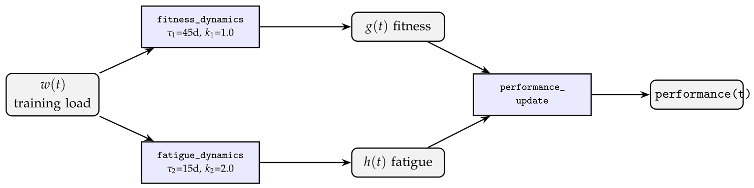
Banister two-compartment fitness-fatigue mechanism, coefficients from Morton 1990, Banister 1975
Boxes denote a dynamics equation and rounded rectangles denote a variable, with the two ends marking input and output, a convention followed by every mechanism diagram in the rest of this paper. drives two independently decaying first-order processes in parallel, which are then subtracted to give performance; the two-compartment framework is taken from Banister et al. [28], with the time constants and gains taken from Morton et al. [27].
Protocols V1, V2: engine integrator numerical accuracy. Full definitions and execution records are in the life-matters-reference-engine repository, test_verification/verification_report.md §2; only the conclusions are summarized here:
- V1, day-by-day comparison against the analytical solution, corresponding to code verification: under constant training load AU/day, the Banister model has a closed-form analytical solution; LM output is compared to it day by day against a 2% threshold.
- V2, step-size convergence check, corresponding to solution verification: independent of the analytical solution, this checks only whether the numerical solution converges monotonically as step_size is refined, catching implementation errors that V1 at a single step size cannot, ones that happen to cancel out only at a particular step size.
On a grid of 6 step sizes, from 1 day down to 30 minutes, and 4 simulation windows, 7, 14, 30, and 60 days, V2 converges monotonically in all 24 cells and passes; V1 passes all 4 windows at step_size ≤ 6h, while the native step_size=1 day passes only for windows of 30 days or longer, failing the 7- and 14-day windows because of the local amplification effect of a difference-type metric described below. Both protocols are treated as passed, and the step_size used in this section and in the subsequent case studies of Section 5.2 and Section 5.3 is never coarser than the granularity confirmed reliable on this grid.
Engine reproduction of the Morton 1990 example. V1 and V2 above each use their own simplified, constant-training-load setup, while the daily_training plan this section actually runs directly reproduces the worked example given by Morton et al. [27]: 60 days of constant load trimps/day followed by complete cessation. The original text directly gives checkpoint numbers for this scenario: on day 60, fitness=3351, fatigue=3044, performance=307; after training stops, performance peaks at 1353 on day 83. Whether this protocol itself can be correctly reproduced by the engine is a further check, complementary to V1/V2, using the model’s actual running step size of hour rather than the synthetic step sizes on the grid above.
Validation parameters: days, days, , ; the performance equation is .
The reference solution is obtained as a piecewise closed-form solution, treating the single daily 09:00 training pulse in this derivation as an approximately constant rate continuous within that phase; the two time constants, 45 and 15 days, are far larger than 1 day, so this approximation holds at the day scale. Under constant w, the solution to the first-order linear ODE is
Phase one, days, , initial condition :
Phase two, days, , pure exponential decay taking , from phase one as initial conditions: , . computed day by day gives the reference-solution column of Table 4; this continuous-time analytical solution is what this section’s Verify criterion actually compares against, a discretization approach not fully equivalent to Morton 1990’s own discrete daily recurrence, and the two approaches’ difference in magnitude is discussed below.
The continuous-time reference solution itself is close to, but not identical to, the discrete daily-recurrence numbers Morton 1990 reports: at day 60 the reference solution gives fitness=3313.8, fatigue=2945.1, performance=368.8, against the reported 3351/3044/307, a relative error of only 1.1% and 3.3% for fitness and fatigue respectively, but performance is a difference of two similarly sized large numbers, so the same absolute error is amplified to 20.1%; the reference solution’s performance peak falls on day 82 at 1353.0, essentially identical to the reported day 83, 1353, a 0.00% difference. The amplification effect does not appear at this checkpoint, because near the peak the fitness and fatigue curves have separated further and are no longer close in magnitude.
The LM engine’s output, compared point by point against this continuous-time reference solution, gives errors of 1.23%, 2.24%, 3.68% on days 1, 5, and 10 respectively, 15.83% on day 30, and 22.26% on day 60, all a continuation of the “performance as a difference of two close large numbers” effect above, not integration error; the engine’s own performance peak falls on day 81 at 1383.4, a 2.33% error against the continuous-time reference solution’s day-82 value of 1353.0, settling back to 823.4 at the simulation endpoint on day 119, a 1.45% error against the reference solution.
The error is not uniformly below 2%: days 30 and 60 reach 15.83% and 22.26% respectively, exceeding the threshold and more pronounced than the early days 1/5/10. This is the same mathematical effect as the local amplification seen in the V1 grid above: performance = fitness − fatigue is a difference between two growth quantities of similar magnitude, and the relative error is amplified whenever the two are close in value and the difference passes near a local minimum, even though fitness and fatigue as individual state variables each keep their own error within single-digit percentages over the same period. Concretely, at day 60 the fitness and fatigue relative errors are 0.82% and 3.71% respectively; performance’s 22.26% is the result of amplifying the difference between the two, not a failure of the Euler integration itself. By day 81, near the peak, the two curves have separated further, the difference is no longer near zero, and the error falls back to 2.33%, falling further to 1.45% by day 119.
The performance peak falls on day 81 at 1383.4 AU; the independent continuous-time reference solution’s peak falls on day 82 at 1353.0 AU, consistent with the day 83, 1353 AU that Morton et al. [27] report directly in their text. This checkpoint happens to fall in the region where the fitness/fatigue curves have separated the most and the amplification effect is weakest, where this section’s discretization difference shows up least.
Figure 1 compares the LM format engine’s output against the independent continuous-time reference solution. Fitness, fatigue, and performance share a vertical axis in AU, with simulation days on the horizontal axis; solid lines are engine output, dashed lines the reference solution. A grey vertical line marks the end of training at day 60; performance peaks at day 81, 1383 AU, closely matching the day 83, 1353 AU that Morton et al. [27] report. The performance curve dips briefly below zero early in training, consistent with the behavior the original paper itself describes, fatigue rising faster than fitness early on. Engine output matches the independent reference solution point by point, with the error range in Table 4; this verify result for the LM reference engine is correct.
4.3. Declaration-Layer Checks: Epidemiological RR Effect-Size Family and Clinical-Psychology Cohen’s d Effect-Size Family
Section 4.2 checks the numerical integration accuracy of continuous dynamical equations; this section checks a mechanism of an entirely different nature: LM format allows an effect size itself, a relative risk, hazard ratio, or standardized effect size, to be declared directly inside variables, tagged by its statistical type through an evidence_type field. Section 2.2 already gives the complete definition of this conversion, the conversion equation and required auxiliary field for each of 8 evidence_type values including OR/HR/RR/Cohen’s d; this section does not repeat that table and checks numerically only the two families actually used here, RR/HR and Cohen’s d. The checking method differs accordingly: each case declares an effect size from real literature together with an illustrative baseline value, lets the engine compute a result by the conversion rule given in Section 2.2’s table, and checks it digit by digit against a hand-computed expected value. This is not an independent prediction; the number being checked is itself the target being verified. Its value lies in demonstrating that the conversion field defined in Section 2.2 can be correctly parsed and correctly converted by the engine, and that this mechanism is not limited to medical effect-size notation, covering both epidemiology’s relative-risk/hazard-ratio convention and psychology’s standardized-effect-size convention.
For the epidemiological RR/HR effect-size family, the conversion rule is that exposed-group risk equals baseline risk times the effect size:
Table 5.
RR/HR effect-size conversion checks
| Case | Lit. effect size | Baseline risk | Engine output | Judgment |
| Smoking–lung cancer mortality | RR=24.97 | 0.6% | 14.98% | Exact, 0.6×24.97 |
| Processed meat–all-cause mortality | RR=1.15 | 1.0% | 1.15% | Exact match |
| Processed meat–colorectal cancer | RR=1.18 | 1.0% | 1.18% | Exact match |
| Inactivity+short sleep–all-cause mortality | RR=1.42 | 1.0% | 1.42% | Exact match |
| Chronic hepatitis B–hepatocellular carcinoma | RR=223 | 0.3% | 66.9% | Exact match |
| Waist circumference–lung cancer | RR=1.10 | 0.6% | 0.66% | Exact match |
For the clinical-psychology Cohen’s d effect-size family, population_sd is currently 1.0 for all three cases, so the conversion rule degenerates to pass-through, checking only whether the field is read out and displayed correctly, a more basic check than the RR/HR family’s multiplicative conversion:
Table 6.
Cohen’s d effect-size conversion checks
| Case | Lit. effect size | Engine output | Judgment |
| CBT for depression, Cuijpers et al., 409-trial, 52,702-patient meta-analysis | d=0.79 | 0.79 | Exact match |
| Mindfulness for mood, Hofmann et al. 2010 | g=0.59 | 0.59 | Exact match |
| Mindfulness for anxiety, Hofmann et al. 2010 | g=0.63 | 0.63 | Exact match |
The complete literature source, confidence interval, and modeling field definitions for each of these 9 effect sizes are given in the description inside the corresponding model file, with full citation traceability in models/papers/s1/declarative_evidence/reference/evidence.bib. The 9 files themselves live under models/references/, organized by discipline, as general reference components that run independently of any paper; a further 9 identically named _case.yaml wrapper files let readers and reviewers confirm directly under papers/ that these 9 cases are available in the S1 build, and the engine’s actual output matches the table above digit for digit.
5. Validation: Case Studies
5.1. Validation Framework
Taking verify as already established, this section checks whether the results of a joint simulation are self-consistent and can support a real decision. Sargent [17] defines validation as checking whether a model’s structure and parameters represent the real system accurately enough for its intended use; this paper makes that definition concrete as a single criterion: validation does not ask whether a single curve interpolates accurately, but whether, once multiple independently calibrated dynamics are coupled together in simulation, the joint behavior of the variables is self-consistent and produces a real, discriminating Pareto front that supports a concrete decision, a criterion different from the single-variable, single-declaration objects verified in Section 4, so the same curve-fitting style of check cannot be reused here.
The standard definition of Pareto dominance is from Miettinen [29]: one solution dominates another if and only if it is no worse on every objective and strictly better on at least one, and the Pareto front consists of the non-dominated solutions. Whether a free decision variable will cause the front to degenerate is read from the sign of its marginal effect on each objective: when the signs agree, the front degenerates to a boundary corner of that variable; when the signs are opposite, the front instead shows a continuous, discriminating tradeoff distribution. Section 5.2 and Section 5.3 each derive this sign relationship from their own equations and then check the numerical optimization result against that expectation; Section 5.4 summarizes the classification for both case studies together with the two verification case studies from Section 4.
The CKD and aircrew case studies show that optimization results themselves can be reliably produced, but different disciplines are not at the same level of theoretical maturity for the same class of decision problem, and the same body of literature evidence, processed under different modeling choices, can produce fronts pointing in entirely different directions, a point Section 5.4 illustrates concretely with a framework comparison outside the two case studies themselves. LM format writes every modeling choice, together with its derivation, into an executable, version-tracked file, providing a shared platform for cross-disciplinary peer checking of these choices. What this paper’s validation actually evaluates is the LM model itself: whether a discipline’s claim can be encoded as an executable model and stay self-consistent under multi-disciplinary joint simulation; the paper only supplies the claims and the numbers, and is not itself the object being evaluated. Self-consistency alone is not sufficient evidence; it is also necessary to check whether the joint result falls near an external benchmark independent of the modeling process, such as a safety threshold given by a current clinical guideline.
The two case studies each test, under a different coupling condition, whether joint simulation can produce a real, non-degenerate front: the CKD case couples two conflicting clinical guidelines within the same specialty, while the aircrew case swaps in a discipline combination with no shared literature base at all, testing whether front degeneration depends on the modeling choices themselves.
5.2. CKD Protein-Muscle Tradeoff Model
A chronic kidney disease patient faces two mutually contradictory specialty recommendations: nephrology wants protein intake as low as possible to slow GFR decline, with the KDIGO 2020 clinical practice guideline [30] recommending 0.6 to 0.8 g/kg daily; geriatric medicine and sarcopenia management want intake as high as possible to preserve muscle synthesis, with the PROT-AGE consensus [31] recommending at least 1.0 g/kg/day; the two recommended ranges do not overlap at all. The timing of the switch from a restriction phase to a maintenance phase is a third decision dimension neither guideline has ever discussed, and the optimal choice is driven jointly by the thresholds of two physiological trajectories, GFR and muscle mass, and by the trajectory of a patient’s dietary adherence decaying over time. The runnable model file for this section is ckd_protein_sim.yaml, with three optimization scenarios in the same directory, ckd_protein_opt_renal.yaml, ckd_protein_opt_muscle.yaml, ckd_protein_opt_joint.yaml.
The model couples three independently calibrated dynamics: GFR decline is driven by protein load aggravating the burden on residual nephrons, with the sensitivity parameter taken from Kasiske et al.’s [32] meta-analysis of 13 randomized controlled trials; muscle-mass synthetic-metabolism rates are calibrated from Carrero et al. [33] and Wang and Mitch [34]; a patient’s dietary adherence decays continuously with the length of the restriction phase, with the rate taken from Rizzetto et al.’s [35] real longitudinal data on 3-year adherence in CKD low-protein-diet patients, and adherence recovers when a maintenance-phase meal is triggered, with qualitative support from Westenhoefer et al.’s [36] comparison of flexible and rigid dietary restraint. Actual intake, rather than the prescribed value, enters both the GFR and muscle-mass dynamics, so the longer the restriction phase runs and the more adherence decays, the more the prescription’s real physiological effect is discounted.
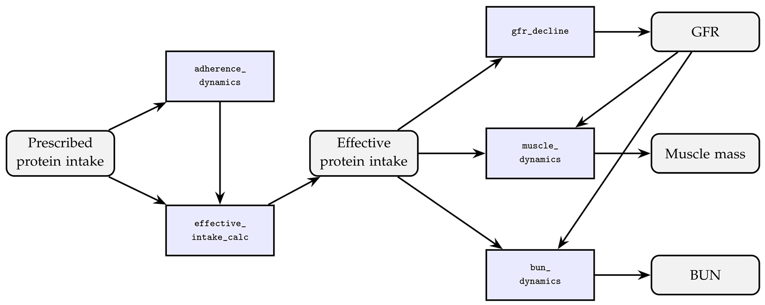
CKD protein-muscle tradeoff mechanism, coefficients from Rizzetto 2017, Westenhoefer 1999, Bauer 2013, Kasiske 1998, Carrero 2013, Moore 2015, Wang and Mitch 2014
Writing p for actual per-meal protein intake, g/kg for the injury threshold, for the sensitivity coefficient, and G for GFR, the gfr_decline equation gives
Writing m for muscle mass and for the synthetic efficiency coefficient, the muscle_dynamics equation gives
The two partial derivatives have opposite signs: the closer protein intake sits to the search’s lower bound, the more GFR is protected and the more muscle mass is lost, and the reverse holds toward the upper bound, so the two objectives cannot both be optimal at the same intake level. The joint optimization’s Pareto front should therefore show a continuous, monotonically opposed distribution between intake and the two objectives, GFR and muscle mass, not degenerating to a single point.
The control variables are the three meals’ protein intake, together with the restriction-to-maintenance switch timing itself set as an optimization object, the K×4 T4 dimension. Three optimization scenarios, a nephrology single-specialty run maximizing GFR, a rehabilitation single-specialty run maximizing muscle mass, and a joint multi-specialty run maximizing both together with lm_score, all import the complete equation set of ckd_protein_sim.yaml through imports.
Figure 2.
CKD protein-muscle tradeoff optimization results, four panels; the six plans’ colors and line styles correspond to Table 7, with static baselines as dotted/dashed lines and optimized results as solid lines. (a) GFR trajectory. (b) Muscle-mass trajectory. (c) Joint Pareto front, GFR vs. muscle mass, n=9. (d) The joint multi-specialty plan’s optimal protein-intake calendar, with a black dashed line marking the week-27 restriction-to-maintenance switch. Panel-by-panel detail in ckd.md.
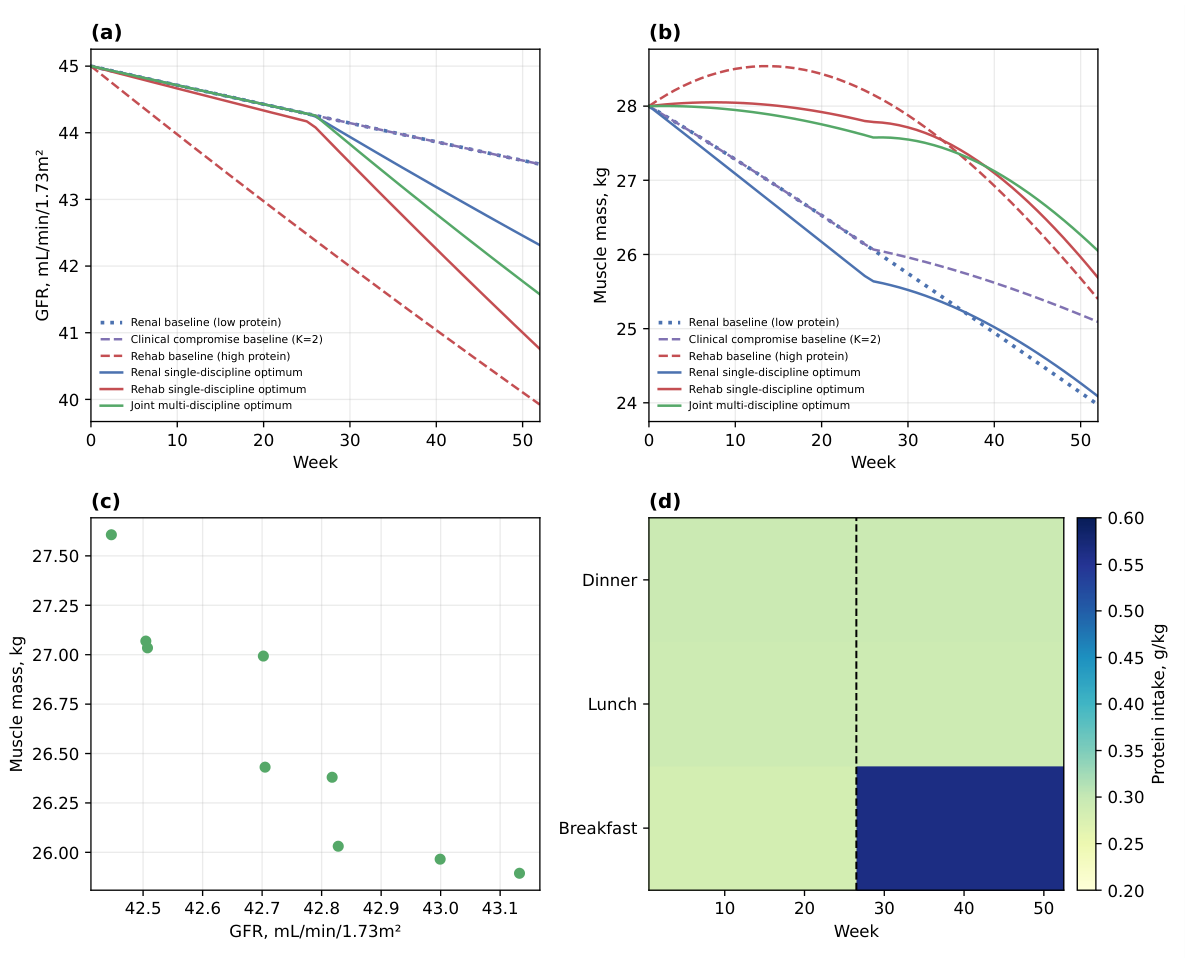
Table 7.
CKD protein-intake plan comparison, week-52 endpoint values. GFR in mL/min/1.73m2
| Plan | Protein-intake configuration | Time-avg. intake | GFR | Muscle mass, kg |
| Nephrology baseline, sustained low protein, unsegmented | AM 0.22+noon 0.21+PM 0.22 g/kg | 0.65 g/kg/day | 43.53 | 24.31 |
| Clinical compromise baseline, K=2, 26wk restriction then 26wk maintenance | Restriction 0.65→maintenance 0.84 g/kg | 0.745 g/kg/day | 43.53 | 25.43 |
| Rehabilitation baseline, sustained high protein, unsegmented | AM 0.38+noon 0.36+PM 0.37 g/kg | 1.11 g/kg/day | 39.92 | 25.40 |
| Nephrology single-specialty optimum, GFR only | AM 0.17+noon 0.20+PM 0.22 g/kg, +0.29 from maintenance | ≈0.59→0.88 g/kg/day | 42.23 | 24.24 |
| Joint multi-specialty optimum, K×4: GFR+muscle mass+lm_score | AM 0.28+noon 0.29+PM 0.29, +0.28 from maintenance | ≈0.87→1.15 g/kg/day | 41.49 | 26.20 |
| Rehabilitation single-specialty optimum, muscle mass only | AM 0.31+noon 0.30+PM 0.29, +0.42 from maintenance | ≈0.91→1.32 g/kg/day | 40.74 | 25.75 |
Without LM, a physician can only choose between the nephrology baseline and the rehabilitation baseline, the former pushing muscle mass down to 24.31 kg to hold GFR at 43.53, the latter pushing GFR down to 39.92 to hold muscle mass at 25.40 kg, with no third option and no tool telling the physician which week to switch from restriction to relaxation. The joint multi-specialty optimum reaches GFR 41.49 and muscle mass 26.20 kg, 1.57 higher on GFR and 0.80 kg higher on muscle mass than the rehabilitation baseline, achieved by converging the restriction-to-maintenance switch, a timing dimension neither guideline discusses, to around weeks 26 to 27. BUN falls within 10.36 to 19.33 mg/dL across all six plans, meeting the ≤20 mg/dL clinical safety constraint. This conclusion is presently only a preliminary, qualified inference based on this paper’s two endpoints and current literature parameters, not directly usable for a clinical prescription, and still requires nephrology and geriatric-medicine specialists to perform a finer-grained group assessment tailored to individual patients.
Limitations: the muscle-mass synthetic-metabolism term now includes the saturation point for single-meal myofibrillar protein synthesis in older men, 0.40±0.19 g/kg body weight, reported by Moore et al. [37], as an upper bound, but the real resistance-exercise gating mechanism is not included in this model; the model does not include a mortality endpoint; and the dietary-adherence decay rate is extrapolated from a single follow-up timepoint’s adherence proportion, not a direct measurement of a continuous decay function.
5.3. Aircrew Cross-Timezone Scheduling: Layover Recovery Versus On-Duty Fatigue Tradeoff
Between every cross-timezone round trip a long-haul international flight crew flies, an airline’s scheduling department has to settle on a specific number of layover-recovery days, currently mostly by experience, without ever having quantitatively linked the number of recovery days to the crew’s actual circadian state. Aviation-medicine fatigue modeling and crew-scheduling operations research are each mature fields on their own, but no directly corresponding cross-over work was found; the closest is Serkh and Forger [38], who use the same circadian pacemaker model for optimal light-exposure control, but with only a resynchronization-time axis and no cost axis.
Lengthening the layover recovery period lowers the fatigue proxy on the day of the return duty, but increases the crew’s total days away and, with it, operating cost. The joint optimization objective is to simultaneously minimize trip_cost_days, the crew’s total days away, and circadian_misalignment_proxy, the fatigue proxy on the first duty day after return; the two decision variables are the number of layover-recovery days L, 1 to 5 days, and the light-exposure timing H, local clock 4 to 22. The model’s core coupled mechanism is the Forger-Jewett-Kronauer circadian pacemaker model: the main-oscillator Process P’s equation structure is taken from Jewett, Forger, and Kronauer [39], and the light-drive chain Process L’s equations are taken from St Hilaire et al. [40]; the standard parameter set is mostly taken via Rea et al. [41], while G, , and the intrinsic period hours instead take St Hilaire et al.’s [40] and Czeisler et al.’s [42] own revised/independently calibrated values respectively. The runnable model file for this section is aircrew_circadian_sim.yaml, with the joint optimization in aircrew_circadian_opt.yaml.

Aircrew circadian tradeoff mechanism, light-response pathway from St Hilaire 2007, pacemaker from Jewett 1999
L enters the cost objective through trip_cost_update; H and L appear together in total_light_update, which determines total light intensity, and this signal travels down the Process L chain to become , the modulated drive on the pacemaker’s main oscillator. An eastbound trip requires the pacemaker to complete a phase advance, and the sole source of asymmetry is the free-running phase-delay bias produced by the intrinsic period being slightly greater than 24 hours, precisely the mechanism by which the model rederives eastbound recovery as harder without any bolted-on directional coefficient. The light drive’s partial derivative is a state-dependent gain factor, spanning roughly a 3.9-fold range based on amplitudes measured during diagnostic-phase scanning; trip_cost_update gives , with always positive and independent of light timing. It can therefore be expected that cost rises linearly with the recovery period, the fatigue proxy falls monotonically with diminishing marginal returns as the recovery period lengthens, and light timing should favor the morning to maximize the gain factor’s drive effect.
The joint optimization searches with NSGA-II over a space of 1 to 5 recovery days and light timing 4 to 22, population size 100, 200 generations, finding 100 non-dominated solutions, all mutually non-dominating, with a continuous front and no single-point degeneration. trip_cost_days = layover_days + 2.0 holds exactly; light timing converges entirely between 13.11 and 14.89, tight against noon into early afternoon, not in the predicted morning region; checked against outside literature, this convergence region happens to fall exactly within the window Sack’s [43] clinical jet-lag guidance recommends for avoiding morning light and seeking afternoon light in the first few days, so what was wrong was the case’s initial qualitative prediction, not the model itself; the fatigue proxy falls overall with the recovery period but shows a small local uptick in the 2.5 to 3.0-day range. Table 8 lists 5 representative points spanning the full range of the front.
Against current scheduling practice, a fixed 3-day recovery period, light timing defaulting to noon, no structured intervention, at nearly the same operating cost the joint optimization lowers the fatigue proxy from 0.951 to 0.856, with light timing alone contributing roughly six-tenths of the improvement, and its contribution grows significantly larger as the recovery period lengthens, negligible when the recovery period is itself very short.
Table 9.
Non-LM baseline versus LM joint optimization, a pair of solutions with similar operating cost
Table 9.
Non-LM baseline versus LM joint optimization, a pair of solutions with similar operating cost
| Scenario | Layover days | Light timing | trip_cost_days | circadian_misalignment_proxy |
| Non-LM baseline, 3-day threshold, light unoptimized | 3.00 | 12.00 | 5.00 | 0.951 |
| LM joint optimum, closest-cost solution on the front | 3.11 | 14.03 | 5.11 | 0.856 |
Checked against the equation-derived predictions: cost rising linearly with the recovery period matches exactly; the fatigue proxy falling with the recovery period matches in direction but shows local fluctuation; light timing favoring the morning is not supported in direction, though its contribution in magnitude is far from negligible, reported honestly, with no retroactive rewriting of the derivation. Figure 3 panels (a) and (b), the sim trajectory panels, show this dynamics directly. Panel (a) shows alertness_proxy completing the pacemaker’s own convergence toward the limit cycle during the recovery period; the 1.5-day, 3-day, and 4-day return lines fall respectively near the rising edge, the falling edge, and the trough of that oscillation, so the phase at which the return moment lands moves non-linearly with recovery length, in the same direction as the local uptick the diagnostic scan finds at finer day intervals, not a discretization artifact. Panel (b) compares light at noon against light at 08:00 under a fixed 3-day recovery period; the two curves nearly coincide for almost the whole simulation, diverging only at the trough inside the 24-hour post-return window, where the 08:00 plan bottoms out at 0 and the noon plan stops around 0.05, the small amplitude gap behind the 1.000 versus 0.951 fatigue-proxy values above, and a direct illustration of why an effect of this magnitude is easy for a directional prediction to miss. One possible reason is that circadian_misalignment_proxy is driven jointly by phase alignment and the pacemaker’s instantaneous amplitude, so a light pulse landing in the afternoon rather than the morning can still bring improvement by suppressing the instantaneous amplitude, a conjecture not yet verified by independently extracting the pacemaker’s phase angle.
Limitations: the photoreceptor state’s time constant is close to the simulation step size, and Euler discretization may not resolve this fastest dynamic well enough; light timing is fixed at a single moment for the whole recovery period rather than adjusted day by day as a true phase-response curve would require; the model does not represent the outbound leg’s timezone jump, homeostatic sleep pressure, or multi-leg sleep-debt accumulation, the main reason this case study is positioned as a feasibility demonstration rather than something that can directly support a scheduling decision.
Both case studies use LM format in the forward direction, literature parameters plus a behavioral plan yielding an optimal Regimen; LM format also supports another mode of use, loading multiple independent literature parameterizations of the same physiological or pharmacological process into one framework and checking the shape of their joint feasible region, Simulation-as-Validation, which this paper does not develop further; candidate cases are recorded in validation_report.md for reference and as material for future research.
5.4. Qualitative Classification of Case-Study Structure
Section 5.1 has already given the criteria for Pareto dominance and front degeneration; Section 5.2 and Section 5.3 have each derived a sign relationship from their own equations; this section places the two case studies alongside the two verification case studies from Section 4 and reads off each one’s structural class.
Section 4.2 and Section 4.3 carry no optimization block and belong to numerical-accuracy verification and declaration-layer checking respectively; they produce no Pareto front, and the classification framework does not apply to either.
Section 5.2 derives from its equations that the partial derivatives of protein intake with respect to GFR and muscle mass have opposite signs, predicting a front that shows a continuous, monotonically opposed distribution between intake and the two objectives. Table 7 and Figure 2 confirm this prediction, with muscle mass rising from 25.89 to 27.61 kg as protein intake rises, constituting a real tradeoff against the GFR objective, with a mild tradeoff magnitude.
Section 5.3 derives three predictions from its equations: trip_cost_days should be exactly linear in the recovery period, independent of light timing; circadian_misalignment_proxy should fall monotonically with diminishing marginal returns as the recovery period grows; and the optimal light timing should favor the lower-bound morning end of the search space. Figure 3 confirms the first; partially confirms the second, with the fatigue proxy falling overall but a small local uptick in the 2.5 to 3.0-day range; and does not confirm the third in either direction or magnitude, with light timing converging entirely near noon into early afternoon rather than the morning, and its contribution in magnitude far larger than predicted, an example where both the direction and the magnitude prediction miss, but in strikingly different ways, reported honestly with no retroactive rewriting.
This classification method also applies when drafting a new model’s equations: once the equations are finalized, the marginal-effect sign of each free decision variable on each objective can be derived directly, predicting the front’s structure before running the optimizer, and then checked against the numerical optimization result, establishing a clear causal-checking relationship between equation design and numerical validation.
6. Discussion
6.1. LM Format as a Mechanism-Orchestration Format
VESO determines that what LM format solves is the layer of connecting mechanisms already scattered across the published literature, each unaware of the others, into one runnable system, see Section 1.1; behavioral intervention decision-making is the first application domain this paper chose, because an executable life or clinical plan naturally has to pass through physiological, psychological, social, and economic constraints from several subsystems at once, see Section 1.2. K×4 is this application domain’s concrete representation of a decision result landing in calendar structure, not the full range of scenarios this orchestration structure itself can cover. Neither VESO nor K×4 refers to any health-specific construct; any simulation in which separately published mechanisms share a decision variable, and in which the decision is a segmented periodic schedule, has the same structure. The operations-scheduling side of the aircrew case in Section 5 is one such instance, and domains such as maintenance planning or staff rostering are candidates this paper does not test.
The two feasibility-demonstration case studies of Section 5, a CKD protein-muscle tradeoff model at the intersection of nephrology and nutrition, and an aircrew cross-timezone scheduling model at the intersection of aviation medicine, chronobiology, and operations scheduling, together show why the decision layer must exist as an independent formal layer: the cross-disciplinary constraints involved typically exceed the design scope of any single-discipline sub-model format; they need an above-the-model language to combine sub-models from different disciplines into a single optimizable object, and that is the layer LM format provides.
VESO’s framework also does not stop at LM format, and is not confined to YAML as a carrier; other tools and implementations are equally free to draw on it. This paper chooses YAML because both researchers without a programming background and large language models can read and write it directly, and adjust it flexibly.
6.2. Limitations
Determining the number of segments K: K is currently judged by the modeler from how many clinically distinguishable execution phases a plan contains, not a numeric hyperparameter automatically searched by an information criterion, see Section 2.7; this judgment depends on the modeler’s domain knowledge, and no systematic tooling assists it yet. A mathematical method to assist this judgment is a possible future direction; this paper only proposes the framework at an early stage and has not yet explored this direction in depth.
Weekday-anchored periodicity: is defined as a subset of weekdays, covering “every day,” all seven, and “several times a week,” any combination of weekdays. This periodicity is set by social life rhythms, the workday/weekend structure, the main scenario this paper’s K×4 case studies cover, but it does not express a pure day-interval periodicity unrelated to weekday structure and instead set by a physiological or pharmacokinetic rhythm, such as strict every-other-day dosing; this is a real scenario the reference engine does not yet implement, requiring an extension to days semantics or a new dedicated field, left as future work.
Euler integration accuracy: for sub-day-scale fast dynamics, such as minute-level glucose changes, Euler integration at day may not be accurate enough. LM format 1.0 is explicitly positioned at the day-to-month-scale behavioral model; sub-day scenarios are recommended to use a smaller step size or wait for the higher-order integration options planned for LM format 1.1.
No RCT clinical validation: every optimization result is a computer-simulation product, hypothesis-generating in nature, and does not constitute clinical advice. Before an LM format optimized plan is used in an actual patient intervention, a small-scale RCT is needed to validate the clinical reproducibility of the simulated conclusion.
evidence conversion assumption: the OR → effective RR conversion uses the simplified equation of Zhang and Yu [44], with a smaller error when baseline prevalence is below 10% and a larger error at higher prevalence.
6.3. Future Directions
LM format’s long-term goal is to support cross-disciplinary collaboration in the sense of open science, letting researchers, clinicians, and engineers from different fields extend and validate each other’s models on the same format and toolchain, rather than each developing an incompatible representation in isolation. The author will continue to pursue the following directions at the LM Reference Engine level, serving the format’s own ease of use and barrier to participation:
- A parameter-calibration interface, the inner-loop Modeller: calibrating the literature-derived initial parameters in variables to a specific individual or cohort, letting researchers without a programming background complete this step without writing their own scripts.
- Model-combination constraints: required or forbidden combination relationships within imports, reducing invalid or contradictory configurations that arise from oversight when researchers combine sub-models from different disciplines, making cross-disciplinary combination more reliable.
7. Conclusion
This paper reports LM format 1.0, an open specification that organizes mechanisms, effect sizes, thresholds, and constraints scattered across different disciplinary literatures into a runnable system, with a core structure of four VESO actions running through the entire format, see Section 1.1. Behavioral intervention decision-making is the first application domain this paper chose, addressing a gap in existing modeling formats for cross-disciplinary coupled individual health decisions, see Section 1.2. LM format is a self-sufficient primary modeling format: a single YAML file can describe a model’s mechanisms, simulation experiments, multi-objective optimization, and an executable intervention plan.
LM format’s core contributions are:
- 1.
- VESO: a mechanism-orchestration structure running through the entire format, organizing cross-disciplinary effect sizes, equations, thresholds, and constraints into a runnable, optimizable, checkable system-science object, providing a common foundation for cross-disciplinary research collaboration and a lightweight paradigm for an AI system to organize the domain knowledge it needs to compute against.
- 2.
- A decision-oriented variable system: three variables classes, state, input, parameter, layered with an orthogonal evidence_type attribute that converts a literature effect size in place, clearly distinguishing a quantity the executor controls, an individual characteristic parameter, a physiological state output, and a literature effect size, so that variable type and optimization semantics correspond strictly.
- 3.
- K×4 Regimen plus the iCal bijection theorem: within the behavioral-intervention application domain, reducing the optimization search space from to , a 30- to 120-fold reduction, while guaranteeing at the level of the formal definition that output is invertibly mappable to a standard calendar file within a restricted iCal profile. Optimization output is, by construction, encodable as a standard calendar file within this profile.
- 4.
- Publishable optimization results, optimization.results: a Pareto front embedded in a YAML model file, so publishing a model publishes its results, supporting warm-start continuation and one-click reproduction of multiple plans.
- 5.
- A FAIR-aligned, format-first open ecosystem: the format is the contract; the library is just an example. A strict specification paired with an extremely low barrier to participation keeps the cost of contributing close to zero.
Verify confirmed the engine’s numerical correctness, with fitness and fatigue each keeping their own error within single-digit percentages against an independent closed-form analytical reference solution, together with declaration-layer reproduction across disciplines outside medicine such as epidemiology and clinical psychology; Validate, using the CKD protein-muscle tradeoff and aircrew cross-timezone scheduling joint-simulation case studies, confirmed the framework’s ability to connect mutually unaware cross-disciplinary mechanisms into one system and produce a real, non-degenerate decision front, the former reproducing a classic cross-specialty guideline conflict, the latter connecting aviation medicine, chronobiology, and operations scheduling, fields with no prior shared literature base. What the two case studies together demonstrate is the same reproducible capability: given scattered disciplinary evidence, LM format can assemble it into an executable, optimizable joint simulation that independent peers can check, not limited to any one particular combination of disciplines.
The native causal-DAG field causal_dag and its integration with a causal-inference toolchain [45], together with a mathematical method to assist multi-candidate K-value determination, are the two open directions this paper considers properly part of LM format’s specification level and worth pursuing further; both remain at the conceptual stage for now. Early use has also shown that an AI agent can understand and construct VESO-structured models, using the LM CLI to run simulation and validation and to repeatedly check and correct its own estimates; the systematic effectiveness of this mode of collaboration is left to future evaluation.
LM format 1.0’s specification and reference model library have been released at https://github.com/shenfan19/life-matters-models under a CC BY 4.0 license, for free use and contribution by researchers in biomedical modeling, clinical systems science, and cross-disciplinary health-decision research; the LM Reference Engine’s source code is public at https://github.com/shenfan19/life-matters-reference-engine, with access details given in Data availability.
Funding
This research did not receive any funding.
Ethical Considerations
This study did not involve human participants, human data, or human tissue. All model parameters are taken from previously published literature, and ethical approval was not required.
Consent to Participate
Not applicable.
Consent for Publication
Not applicable.
Data Availability Statement
The LM format 1.0 specification document is published at https://github.com/shenfan19/life-matters-models/blob/main/docs/LM_format_1.0.md, and the reference model library at https://github.com/shenfan19/life-matters-models, both under a CC BY 4.0 license. The LM Reference Engine’s source code is published at https://github.com/shenfan19/life-matters-reference-engine. The model equations, parameters, and scientific conclusions of the validation case studies this paper reports, all cases in Section 4 and Section 5, have been checked and confirmed by the author personally, and the scope of AI-assisted tool use is described in the Acknowledgments section. The reference model library holds more content than this paper cites; most model files in the library are AI-assisted in origin, have had a preliminary review, and have not yet been checked by a domain expert. Readers citing content from the model library beyond this paper should judge its credibility accordingly and should not assume that publication implies validation. A model file’s domain-content accuracy check is independent of the LM format compliance determination defined in Section 2.1: each parameter’s literature source is recorded in its own variables.<name>.reference field, and an outside researcher checking or revising one parameter does not need to understand the reference-engine implementation or modify any other model file. Researchers who need to cite content produced by this project should cite the corresponding paper itself; a model YAML file does not constitute an independent scholarly citation unit and serves as the paper’s reproducibility material, accessible through the URLs above.
Acknowledgments
The author used AI-assisted tools during the preparation of this work for coding assistance, automated testing, documentation, and drafting and revising portions of the manuscript text. All model equations, parameter values, and scientific conclusions were determined by the author, who reviewed all AI-assisted output and takes full responsibility for the accuracy and originality of the manuscript.
Conflicts of Interest
The author(s) declared no potential conflicts of interest with respect to the research, authorship, and/or publication of this article.
References
- Petty, M.D.; Weisel, E.W. A composability lexicon. In Proceedings of the Spring Simulation Interoperability Workshop, Orlando, FL, March 30–April 4; 2003; pp. 181–187. [Google Scholar]
- Zeigler, B.P.; Praehofer, H.; Kim, T.G. Theory of Modeling and Simulation: Integrating Discrete Event and Continuous Complex Dynamic Systems, 2nd ed.; Academic Press: San Diego, 2000. [Google Scholar]
- Fu, M.C. Optimization for simulation: Theory vs. practice. Inf. J. Comput. 2002, 14(3), 192–215. [Google Scholar] [CrossRef]
- McEwen, B.S. Stress, adaptation, and disease: Allostasis and allostatic load. Ann. N. Y. Acad. Sci. 1998, 840(1), 33–44. [Google Scholar] [CrossRef] [PubMed]
- Kivimäki, M.; Nyberg, S.T.; Batty, G.D.; et al. Job strain as a risk factor for coronary heart disease: a collaborative meta-analysis of individual participant data. The Lancet 2012, 380(9852), 1491–1497. [Google Scholar] [CrossRef] [PubMed]
- Choi, K.; Medley, J.K.; König, M.; et al. Tellurium: An extensible Python-based modeling environment for systems and synthetic biology. Biosystems 2018, 171, 74–79. [Google Scholar] [CrossRef] [PubMed]
- Hucka, M.; Finney, A.; Sauro, H.M.; et al. The systems biology markup language, SBML: a medium for representation and exchange of biochemical network models. Bioinformatics 2003, 19(4), 524–531. [Google Scholar] [CrossRef] [PubMed]
- Lloyd, C.M.; Halstead, M.D.B.; Nielsen, P.F. CellML: its future, present and past. Prog. Biophys. Mol. Biol. 2004, 85(2–3), 433–450. [Google Scholar] [CrossRef] [PubMed]
- von Bertalanffy, L. General System Theory: Foundations, Development, Applications; George Braziller: New York, 1968. [Google Scholar]
- Forrester, J.W. Industrial Dynamics; MIT Press: Cambridge, MA, 1961. [Google Scholar]
- Murphy, S.A. Optimal dynamic treatment regimes. J. R. Stat. Soc. Ser. B 2003, 65(2), 331–355. [Google Scholar] [CrossRef]
- Chakraborty, B.; Moodie, E.E.M. Statistical Methods for Dynamic Treatment Regimes: Reinforcement Learning, Causal Inference, and Personalized Medicine; Springer: New York, 2013. [Google Scholar]
- Nahum-Shani, I.; Smith, S.N.; Spring, B.J.; et al. Just-in-time adaptive interventions, JITAIs, in mobile health: key components and design principles for ongoing health behavior support. Ann. Behav. Med. 2018, 52(6), 446–462. [Google Scholar] [CrossRef] [PubMed]
- Taylor, C.; Munro, A.J.; Glynne-Jones, R.; et al. Multidisciplinary team working in cancer: what is the evidence? BMJ 2010, 340, c951. [Google Scholar] [CrossRef] [PubMed]
- Fritzson, P.; Engelson, V. Modelica, a unified object-oriented language for system modeling and simulation. Proceedings of ECOOP’98 Lecture Notes in Computer Science, Brussels, Belgium, 1998; volume 1445, pp. 67–90. [Google Scholar]
- Waltemath, D.; Adams, R.; Bergmann, F.T.; et al. Reproducible computational biology experiments with SED-ML: the simulation experiment description markup language. BMC Syst. Biol. 2011, 5, 198. [Google Scholar] [CrossRef] [PubMed]
- Sargent, R.G. Verification and validation of simulation models. J. Simul. 2013, 7(1), 12–24. [Google Scholar] [CrossRef]
- Wilkinson, M.D.; Dumontier, M.; Aalbersberg, I.J.; et al. The FAIR guiding principles for scientific data management and stewardship. Sci. Data 2016, 3, 160018. [Google Scholar] [CrossRef] [PubMed]
- HL7 International. FHIR r5 specification, medicationrequest resource. 2023. Available online: http://hl7.org/fhir/medicationrequest.html.
- Issurin, V.B. New horizons for the methodology and physiology of training periodization. Sports Med. 2010, 40(3), 189–206. [Google Scholar] [CrossRef] [PubMed]
- IETF. Internet calendaring and scheduling core object specification (iCalendar), RFC 5545; IETF, 2009; Available online: https://www.rfc-editor.org/rfc/rfc5545.
- Callen, H.B. Thermodynamics and an Introduction to Thermostatistics, 2nd ed.; Wiley: New York, 1985. [Google Scholar]
- Blochwitz, T.; Otter, M.; Arnold, M.; et al. The functional mockup interface for tool independent exchange of simulation models. In Proceedings of the 8th International Modelica Conference, Dresden, Germany; 2011; pp. 105–114. [Google Scholar]
- Grimm, V.; Berger, U.; DeAngelis, D.L.; et al. The ODD protocol: A review and first update. Ecol. Model. 2010, 221(23), 2760–2768. [Google Scholar] [CrossRef]
- Blank, J.; Deb, K. pymoo: Multi-objective optimization in Python. IEEE Access 2020, 8, 89497–89509. [Google Scholar] [CrossRef]
- Deb, K.; Pratap, A.; Agarwal, S.; et al. A fast and elitist multiobjective genetic algorithm: NSGA-II. IEEE Trans. Evol. Comput. 2002, 6(2), 182–197. [Google Scholar] [CrossRef]
- Morton, R.H.; Fitz-Clarke, J.R.; Banister, E.W. Modeling human performance in running. J. Appl. Physiol. 1990, 69(3), 1171–1177. [Google Scholar] [CrossRef] [PubMed]
- Banister, E.W.; Calvert, T.W.; Savage, M.V.; et al. A systems model of training for athletic performance. Aust. J. Sports Med. 1975, 7(3), 57–61. [Google Scholar]
- Miettinen, K. Nonlinear Multiobjective Optimization; Kluwer Academic Publishers, 1999. [Google Scholar]
- KDIGO 2020 Work Group. KDIGO 2020 clinical practice guideline for diabetes management in CKD. Kidney Int. 2020, 98(4S), S1–S115. [Google Scholar] [CrossRef] [PubMed]
- Bauer, J.; Biolo, G.; Cederholm, T.; et al. Evidence-based recommendations for optimal dietary protein intake in older people: a position paper from the PROT-AGE study group. J. Am. Med. Dir. Assoc. 2013, 14(8), 542–559. [Google Scholar] [CrossRef] [PubMed]
- Kasiske, B.L.; Lakatua, J.D.A.; Ma, J.Z.; et al. A meta-analysis of the effects of dietary protein restriction on the rate of decline in renal function. Am. J. Kidney Dis. 1998, 31(6), 954–961. [Google Scholar] [CrossRef] [PubMed]
- Carrero, J.J.; et al. Etiology of the protein-energy wasting syndrome in chronic kidney disease: a consensus statement from the international society of renal nutrition and metabolism (ISRNM). J. Ren. Nutr. 2013, 23(2), 77–90. [Google Scholar] [CrossRef] [PubMed]
- Wang, X.H.; Mitch, W.E. Mechanisms of muscle wasting in chronic kidney disease. Nat. Rev. Nephrol. 2014, 10(9), 504–516. [Google Scholar] [CrossRef] [PubMed]
- Rizzetto, F.; Leal, V.O.; Bastos, L.S.; et al. Chronic kidney disease progression: a retrospective analysis of 3-year adherence to a low protein diet. Ren. Fail. 2017, 39(1), 357–362. [Google Scholar] [CrossRef] [PubMed]
- Westenhoefer, J.; Stunkard, A.J.; Pudel, V. Validation of the flexible and rigid control dimensions of dietary restraint. Int. J. Eat. Disord. 1999, 26(1), 53–64. [Google Scholar] [CrossRef]
- Moore, D.R.; et al. Protein ingestion to stimulate myofibrillar protein synthesis requires greater relative protein intakes in healthy older versus younger men. J. Gerontol. Ser. A 2015, 70(1), 57–62. [Google Scholar] [CrossRef] [PubMed]
- Serkh, K.; Forger, D.B. Optimal schedules of light exposure for rapidly correcting circadian misalignment. PLoS Comput. Biol. 2014, 10(4), e1003523. [Google Scholar] [CrossRef] [PubMed]
- Jewett, M.E.; Forger, D.B.; Kronauer, R.E. Revised limit cycle oscillator model of human circadian pacemaker. J. Biol. Rhythm. 1999, 14(6), 493–499. [Google Scholar] [CrossRef]
- St Hilaire, M.A.; Klerman, E.B.; Khalsa, S.B.S.; et al. Addition of a non-photic component to a light-based mathematical model of the human circadian pacemaker. J. Theor. Biol. 2007, 247(4), 583–599. [Google Scholar] [CrossRef] [PubMed]
- Rea, M.S.; Nagare, R.; Bierman, A.; et al. The circadian stimulus-oscillator model: Improvements to Kronauer’s model of the human circadian pacemaker. Front. Neurosci. 2022, 16, 965525. [Google Scholar] [CrossRef] [PubMed]
- Czeisler, C.A.; Duffy, J.F.; Shanahan, T.L.; et al. Stability, precision, and near-24-hour period of the human circadian pacemaker. Science 1999, 284(5423), 2177–2181. [Google Scholar] [CrossRef] [PubMed]
- Sack, R.L. Jet lag. N. Engl. J. Med. 2010, 362(5), 440–447. [Google Scholar] [CrossRef] [PubMed]
- Zhang, J.; Yu, K.F. What’s the relative risk? a method of correcting the odds ratio in cohort studies of common outcomes. JAMA 1998, 280(19), 1690–1691. [Google Scholar] [PubMed]
- Pearl, J. Causality: Models, Reasoning, and Inference, 2nd ed.; Cambridge University Press: Cambridge, 2009. [Google Scholar]
Figure 1.
Banister fitness-fatigue two-compartment model
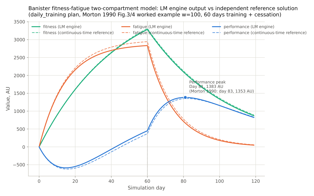
Figure 3.
Aircrew cross-timezone scheduling sim trajectories and joint-optimization results, six panels. Panels (a) and (b) are from –sim output on aircrew_circadian_sim.yaml; panels (c) through (f) are from aircrew_circadian_opt.yaml’s optimizer.results.pareto_front and diagnostic scans over recovery days and light timing. (a) Alertness proxy against simulated time, eastbound, light fixed at noon, comparing 1.5-day, 3-day, and 4-day recovery periods, with a vertical line marking each plan’s own return-flight moment. (b) Alertness proxy against simulated time, eastbound, recovery fixed at 3 days, comparing light at noon against light at 08:00, with the shaded band marking the 24-hour post-return diagnostic window. (c) Joint optimization front. (d) Recovery-days diagnostic scan. (e) Light-timing diagnostic scan. (f) Eastbound/westbound asymmetry comparison. Panel-by-panel detail in aircrew.md.
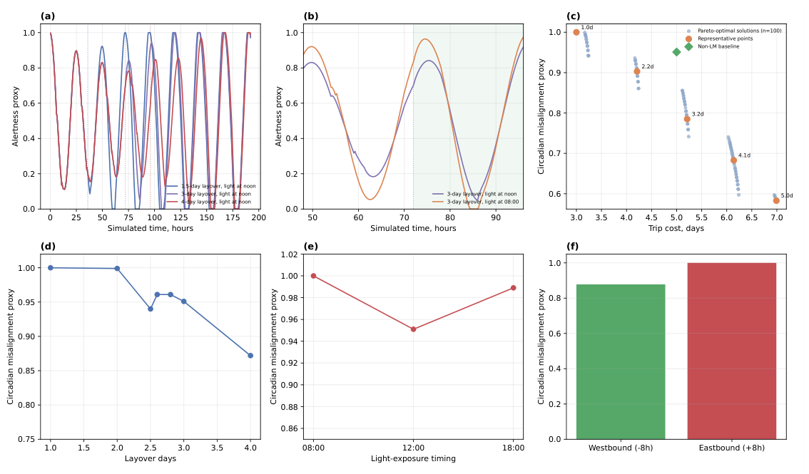
Table 3.
LM format compared with existing modeling languages, by dimension
| Dimension | LM format | SBML / CellML | Modelica | Directly combining existing tools |
| Community-pioneering openness | Plain YAML text, executes directly with no compilation, Section 2.1, Section 2.2 | Read and written through dedicated tools such as COPASI, OpenCOR | Relies on proprietary connector types and a compiled toolchain | Varies by author; provenance is easily lost as code evolves |
| Theoretical permeation | evidence_type maps onto literature statistics, VESO maps onto a systems-science theoretical lineage, Section 1.1, Section 2.2 | Targets the molecular-to-cellular scale only | Targets physical-field coupling only | Varies by script |
| Computational standardization | Three standard interfaces unify simulation/optimization input and output, natively produces a Pareto front, Section 2.2, Section 2.6 | Optimization left to an external toolchain | Optimization left to an external toolchain | Input/output format varies by script |
| Everyday practicality | K×4/iCal bijection maps onto standard calendar events, Section 2.7 | Does not address individual behavioral decisions | Does not address individual behavioral decisions | Varies by script |
| Broad coverage | imports plus step_unit support cross-scale composition, centered on a real individual’s life connecting multiple disciplines, Section 1.1, Section 2.4 | Biochemical-network components accumulated over more than two decades | Industrial component libraries accumulated over decades | Depends on the libraries the author happens to choose |
Table 4.
Numerical comparison of the Banister model’s LM format output against an independent continuous-time reference solution
Table 4.
Numerical comparison of the Banister model’s LM format output against an independent continuous-time reference solution
| Day | LM fitness | LM fatigue | LM perf. | Ref. perf. | Rel. error |
| 1 | 98.7 | 192.1 | -93.4 | -94.6 | 1.23% |
| 5 | 472.0 | 840.7 | -368.7 | -377.2 | 2.24% |
| 10 | 893.8 | 1436.2 | -542.4 | -563.1 | 3.68% |
| 30 | 2177.6 | 2518.0 | -340.3 | -404.4 | 15.83% |
| 60, training ends | 3286.6 | 2835.8 | 450.8 | 368.8 | 22.26% |
| 81, performance peak | 2049.3 | 665.9 | 1383.4 | 1351.8 | 2.33% |
| 119, simulation endpoint | 871.8 | 48.4 | 823.4 | 835.5 | 1.45% |
Table 8.
Representative points on the joint optimization front
| Layover days | Light timing | trip_cost_days | circadian_misalignment_proxy |
| 1.00 | 13.11 | 3.00 | 1.000 |
| 2.21 | 13.54 | 4.21 | 0.903 |
| 3.21 | 14.20 | 5.21 | 0.785 |
| 4.14 | 14.36 | 6.14 | 0.683 |
| 4.99 | 14.40 | 6.99 | 0.583 |
Disclaimer/Publisher’s Note: The statements, opinions and data contained in all publications are solely those of the individual author(s) and contributor(s) and not of MDPI and/or the editor(s). MDPI and/or the editor(s) disclaim responsibility for any injury to people or property resulting from any ideas, methods, instructions or products referred to in the content. |
© 2026 by the authors. Licensee MDPI, Basel, Switzerland. This article is an open access article distributed under the terms and conditions of the Creative Commons Attribution (CC BY) license (http://creativecommons.org/licenses/by/4.0/).
Copyright: This open access article is published under a Creative Commons CC BY 4.0 license, which permit the free download, distribution, and reuse, provided that the author and preprint are cited in any reuse.