
Submitted:
06 October 2026
Posted:
08 October 2026
You are already at the latest version
Abstract
Ozone (O3) pollution exhibits complex processes and characteristics across short-term, seasonal, and long-term temporal scales. Existing studies have predominantly focused on individual scales, highlighting the need for further exploration of response relationships across different scales. This study focuses on East Asia (105° to 125°E, 20° to 42.5°N), integrating daily three-dimensional field data of O3, NO2, HCHO, and isoprene from the ECMWF EAC4 reanalysis dataset, along with ERA5 meteorological data, covering the period from 2017 to 2025. Treating O3 and its major precursors as an integrated analytical object, a dual-layer Gaussian low-pass filter was applied to decompose standardized pollutant fields into short-term (ST), seasonal (SN), and long-term (LT) components. Joint Empirical Orthogonal Function (EOF) decomposition was then employed to extract spatial modes and principal component time series reflecting the co-evolution of ozone and precursors at each scale. PINN was incorporated to explore potential physical drivers underlying each mode, while rolling multivariate Ordinary Least Squares (OLS) regression and CNN-BiLSTM neural network were jointly applied to investigate cross-scale response intensity β and its time-varying characteristics. Results indicate that: (1) modal coupling relationships across temporal scales are continuously evolving, with traditional single-factor dominated patterns giving way to multi-factor synergistic modes; (2) cross-scale interactions are themselves changing, and neglecting their evolution may systematically misestimate risks; (3) only the first long-term mode exhibits a marginally significant upward trend (p = 0.048), while change point detection at 2019 and 2022 closely coincides with major emission reduction policy milestones. Continued cross-scale research is essential for adaptive ozone control strategies.
Keywords:
O3 pollution system
; cross-scale response
; EOF
; CNN-BiLSTM
; PINN
1. Introduction
Since the implementation of the Air Pollution Prevention and Control Action Plan in China in 2013, national PM2.5 concentrations have achieved substantial reductions. However, in the early stages, ground-level O3 pollution received relatively limited attention. To address this issue, the Chinese government has progressively strengthened the coordinated reduction of VOCs and NOx since 2017. The State Council successively issued the Three-Year Action Plan for Winning the Blue Sky Defense War (2018) and the Action Plan for Continuous Improvement of Air Quality (2023), explicitly incorporating ozone control into the national air quality strategy and emphasizing regional joint prevention and control of PM2.5 and O3[1,2,3,4,5].
The formation mechanism of O3 is highly complex, governed by the nonlinear coupling of precursor concentrations, meteorological conditions, and photochemical reactions. This uncertainty renders research spanning from macroscopic ozone variations to microscopic chemical mechanisms all of significant value[6,7,8,9,10,11,12,13,14,15,16]. Ozone concentration variations manifest across multiple scales, including short-term meteorological perturbations, seasonal cycles, and long-term trends. Current research has established an analytical framework covering multiple temporal scales of ozone, encompassing diverse approaches such as time series decomposition, interpretable machine learning, spatial modeling, multifractal cross-correlation analysis, and climate driving factor attribution. He et al. (2025) utilized STL decomposition to quantify the differentiated responses of long-term declining trends and seasonal/short-term perturbations of ozone in the Yangtze River Delta. Zhong et al. (2025) revealed the differentiated climate drivers of interannual variability in heat-ozone compound extreme events between North China and South China through EOF analysis and climate attribution. Ma et al. (2025) and Wu et al. (2026) deepened the mechanistic understanding of short-term extreme ozone events from the perspectives of OVOC photolysis-driven differences in winter and summer formation pathways and nocturnal low-level jet residual layer entrainment processes, respectively. Sowmya et al. (2025) revealed the regulatory role of boundary layer dynamic processes on diurnal and seasonal ozone variations from the perspectives of ventilation coefficient and multifractal cross-correlation[17,18,19,20,21,22,23,24,25,26]. There are many additional studies focusing on ozone at various scales, and we can greatly advance our understanding and knowledge of ozone from previous research.
However, we consider that certain gaps remain in the existing body of work. We suggest that, based on the close chemical linkages between ozone and its precursors, it is worthwhile to attempt treating them as parallel objects for analysis. Furthermore, ozone pollution is essentially a process characterized by time-varying coupling and multi-scale interactions. Nevertheless, existing studies have mostly focused on individual and relatively static relationships, with limited discussion on the dynamic evolution of response relationships across different temporal scales.
This study aims to reveal the evolutionary characteristics of O3 pollution in East Asia from a multi-temporal scale perspective and its responses to emission reduction policies in China. First, O3 and its major precursors are incorporated into a unified covariance matrix for EOF decomposition to extract principal component time series reflecting the co-evolution of pollution, thereby overcoming the limitations of traditional single-pollutant analysis. The principal components are then decomposed into ST, SN, and LT temporal scale components through Gaussian low-pass filtering, and statistical tests are applied to each component to identify potential anthropogenic emission reduction signals. Second, two complementary pathways, OLS and CNN-BiLSTM combined models, are employed to explore the cross-scale response relationship β from larger scales to smaller scales and its time-varying characteristics. A PINN model is further incorporated to conduct exploratory analysis of the potential physical features underlying each mode, thereby enhancing the interpretability of cross-scale response relationships. This study provides a new analytical perspective for deepening the understanding of multi-scale coupling mechanisms of O3 pollution, identifying key response pathways, and evaluating the effectiveness of emission reduction policies across different temporal scales.
2. Materials and Methods
2.1. Data
This study focuses on East Asia (105° to 125°E, 20° to 42.5°N) as the study area. The primary datasets include the following: (1) Three-dimensional field data (0.75°) of O₃, NO₂, HCHO, and isoprene. Previous studies have supported the reliability of these species as representative components of the ozone pollution system[27,28,29,30,31,32,33,34]; (2) Emission data (0.1°) of NOx and VOCs, categorized into four sectors: agriculture, industry, residential, and transportation, along with natural source emission data (0.1°). Both datasets (1) and (2) are derived from the ECMWF EAC4 reanalysis data and global emission inventory data, with the vertical level set at the near-surface 1000 hPa. (3) Six meteorological variables closely associated with ozone: 2-meter temperature, relative humidity, wind speed (WS, synthesized from u and v components), boundary layer height (BLH), daily mean precipitation, and daily surface net upward thermal radiation[35,36,37,38,39]. These data are sourced from the ECMWF ERA5 reanalysis dataset (0.1°). To ensure consistency with the four chemical species for subsequent analysis, area-weighted averaging was applied to regrid meteorological and natural source emission inventory data to 0.75° resolution. The temporal coverage of all datasets spans from January 1, 2017 to December 31, 2025 (daily). Grid-point-wise Z-score standardization was applied to each pollutant, where and σi,j denote the temporal mean and standard deviation at grid point (i,j), respectively. Standardization eliminates the effects of dimensional differences among variables and spatial concentration gradients. Subsequent results primarily reflect anomalous variations of each variable relative to its own historical background.
2.2. Gaussian Filter Decomposition
This study employs a dual-layer Gaussian low-pass filter to decompose the standardized pollutant fields along the temporal dimension. This approach possesses smooth frequency response characteristics and favorable time-domain localization performance. The specific procedure is as follows. (1) A one-dimensional Gaussian kernel with standard deviation σSN=10 days is applied along the time axis as a low-pass filter, yielding the smoothed field GSN(t); (2) A one-dimensional Gaussian kernel with standard deviation σLT=183 days is applied as a second low-pass filter, yielding the long-term smoothed field GLT(t).The short-term component(ST):XST(t) = X − GSN(t), captures weather-scale fluctuations. The seasonal component(SN):XSN(t) = GSN(t) − GLT(t), captures seasonal cycles. The long-term component(LT):XLT(t) = GLT(t), captures multi-year trends. ST, SN, and LT constitute a non-orthogonal decomposition, and the variance proportions of the three components do not necessarily sum to 100%. The sample sizes across the three datasets remain consistent. The Gaussian filter performs frequency decomposition rather than partitioning the dataset into separate blocks.
X(t) = XST(t) + XSN(t)+XLT(t)
2.3. Joint EOF Decomposition
The formation of O3 involves complex underlying causes. By incorporating O3 and its precursor components at each temporal scale after Gaussian filtering into a unified covariance matrix for decomposition, the information is efficiently compressed into a small number of comprehensive modes. While achieving dimensionality reduction, the PC series serves as a composite evolution signal of the ensemble, whose variational characteristics reflect the overall evolution, consistent with the actual behavior of the atmospheric chemical system. The three-dimensional data of each pollutant are reshaped into a “time × space” matrix and then concatenated along the feature dimension to form the joint matrix[40,41,42]:
where s denotes the three temporal scales. The temporal mean is removed from each spatial feature of the joint matrix, and truncated singular value decomposition is applied:
Where PCs is the principal component time series and is the corresponding spatial mode. The spatial modes are fixed and can be understood as stationary concentration distribution patterns manifested by the collective activity of ozone and precursors within the study area. Mode 1 (M1) corresponds to the most frequently occurring distribution pattern, and so forth. Some modes possess clear physical interpretations, while others may represent data residuals. The PC series reflects the temporal activity of each mode. For example, represents the PC series of M1 at the ST scale, and so forth. The explained variance of the m-th mode relative to the total sum of squares of the joint matrix is:
The explained variance reflects the proportion of variance accounted for by the corresponding mode within the entire concentration dataset. The spatial modes from EOF decomposition exhibit alternating positive and negative loading patterns. Positive loading regions (red) should not be simply interpreted as high pollution areas, nor negative loading regions (blue) as low pollution areas. The scientific meaning is derived from the synchronous variation between spatial signs and the corresponding PC values. A grid point is associated with a high ozone concentration component only when the spatial loading and the corresponding PC value share the same sign at a given time. The first two modes at each of the three temporal scales are extracted for subsequent analysis, based on the following rationale. (1) The cumulative explained variances of the first two modes for SN and LT reach 85.40% and 83.48%, respectively, which sufficiently characterize the major spatial variability structures. (2) ST fluctuations are complex and mutually independent, with individual mode variance contributions below 6%. Selecting the first two representative modes that also yield satisfactory deep learning performance reduces uncertainty (SI Section1.2). On this basis, the following analytical indicators are established for the three scales:
(1) For the PC series of each ST mode, the 90th percentile is used as a threshold to identify short-term joint pollution mode anomaly events (adjacent events separated by ≤1 day are merged). Three indicators are computed annually: event frequency (events per year), mean peak intensity (exceedance above threshold), and mean duration (days).
(2) For each SN mode PC series, a harmonic model containing the fundamental frequency and the second harmonic is fitted annually:
PCSN(t) = a0 + a1cos(ωt) + b1cos(ωt) + a2cos(2ωt) + b2cos(2ωt)
Where ω = 2π/365. The following interannual indicators of the seasonal joint pollution mode are extracted: amplitude , peak phase , and mean PC value during the May to September high ozone pollution season.
(3) For the annual mean series of each LT mode PC, the following trend tests are applied. (i) Nonparametric Mann-Kendall test: tests the significance of monotonic trends, reporting the two-sided p-value. (ii) Theil-Sen slope estimate: the median of all pairwise slopes are taken as the robust trend estimator. (iii) Pettitt change point detection: identifies abrupt mean shifts based on the cumulative deviation sequence (, with the test statistic K = max|St|,and significance computed as P = 2exp(−6K2/(n3 + n2)).
2.4. Multivariate Linear Regression and β Series Calculation (OLS)
To further explore the cross-scale response characteristics of the ozone pollution system, two pathways are adopted. The first pathway employs conventional multivariate linear regression (OLS), establishing dynamic linear responses of target scales to driving scales within a 365-day sliding window. A cross-scale response framework from larger to smaller scales is adopted, whereby long-term trends and seasonal cycles serve as relatively stable background states that influence the occurrence frequency and intensity of more rapidly varying short-term events. This assumption is based on the objective of simplifying model structure and avoiding circular dependencies between fast and slow scales that would lead to research complexity and difficulties in interpretation. Two tasks are formulated:
TaskA: PCST(t) = β0 + β1PCSN,M1 + β2PCSN,M2 + β3PCLT,M1 + β4PCLT,M2 + ε
Where PC corresponds to the PC series of each mode. Tasks A and B correspond to the response of ST to LT and SN, and the response of SN to LT, respectively, yielding a total of 12 relationship pairs. Each sliding window requires a minimum of 300 valid sample days. The resulting β series describes the cross-scale dynamic linear response intensity in the sense of conditional correlation. A larger |β| indicates stronger explanatory power of the driving mode over the variation of the target mode. A positive β indicates that the response mode strengthens synchronously when the driving mode intensifies, while a negative β indicates that the response mode weakens when the driving mode intensifies. A positive trend in β indicates that the driving effect strengthens over the years, while a negative trend indicates that the driving effect weakens or reverses direction over the years. All indicators characterize the evolution of relationships rather than the ozone concentration changes resulting from those relationships.
2.5. Cross-Scale Response Modeling
The second pathway employs a CNN+BiLSTM[43,44,45,46,47,48] neural network combination to learn the variational characteristics of all PC series. The model architecture consists of multi-branch one-dimensional CNN and BiLSTM. The CNN contains five parallel convolution branches with kernel widths of 1, 3, 5, 9, and 15 days, respectively, designed to extract local features. The outputs of each branch are processed through GroupNorm and GELU activation before concatenation. The BiLSTM further models the long-range temporal dependencies of multi-scale features. Its output is processed through LayerNorm, residual connections, and a two-layer fully connected network to generate per-timestep predictions. Simultaneously, the CNN produces local response predictions through an independent 1×1 convolution prediction head, which are summed with the BiLSTM output to form a dual-pathway residual output, improving gradient propagation and training stability. For Task A, inputs include PCSN,PCST series along with six meteorological factors. For Task B, inputs include PCLT series along with six meteorological factors. Additionally, for Task A, first−order differences, third−order differences, 7−day rolling standard deviations, and 7−day rolling deviation measures are computed separately for meteorological variables, PCSN,PCST series as derived features to capture the high-frequency variational characteristics at the ST scale, constituting a specialized scheme (SI Section1.3). The model uses PC data from January 1, 2017 to December 31, 2024 for training and leverages the advantages of neural networks to fit the β series, possessing the capability to explore nonlinear cross-scale relationships (in contrast to the analytical solution of OLS). The results are ultimately compared with the β series from the OLS pathway. The year 2025 serves as an independent validation period for predicting that year’s PC and β series, providing a comprehensive assessment of model reproduction and learning capabilities (SI Section 2.1 and Section 2.2).
2.6. PINN Physical Constraint Design
The multi-scale response relationships involve a total of 12 groups of research objects. The secondary variables from EOF decomposition, spatial modes and the corresponding PCs describing each mode, are abstract concepts. It is necessary to make informed judgments and prior assessments regarding the actual physical features that each mode may represent. This study incorporates PINN into the existing neural network architecture, constructing a hybrid attribution framework that integrates data-driven learning with physical knowledge constraints. The PINN embeds six representative fundamental laws of O3-related atmospheric chemistry and physics directly into the loss function as soft penalty terms. During training, these physics-based regularization terms guide the model to search for optimal solutions only within the physically plausible solution space, effectively constraining model behavior without requiring additional labeled data. The PINN first learns physically consistent residual corrections and generates physically regularized feature representations. These physics-enhanced features[49,50,51,52,53,54] are then fed into the neural network for ensemble learning and attribution analysis (SI Section 3.1 and Section 3.2). The specific constraint mechanisms are as follows:
Feature 1: Arrhenius Temperature Factor. Ozone photochemical production involves a series of thermochemical reactions whose rate constants k(T) follow the Arrhenius law:
Where A is the pre−exponential factor, Ea is the activation energy, R is the ideal gas constant, and T is the absolute temperature. This study uses the relative rate factor with respect to a reference temperature Tref(298.15K):
Feature 2: Formaldehyde-to-NO2 Ratio (FNR). The sensitivity of ozone production to precursors depends on the chemical regime. Here, ε is a prescribed constant of 10⁻¹² to prevent division by 0, and 50 serves as the upper clipping limit for the FNR ratio to prevent physically unrealistic extreme values.
Feature 3: O3 Photochemical Production Rate. Here, max(radiation,0) represents the photolysis driving force, corresponding to the radiation value at the relevant grid point. farrhenius(T) is the thermochemical reaction acceleration factor corresponding to Feature 1. VOCsproxyrepresents the total precursor emissions at the relevant location, comprising both anthropogenic and biogenic emission values. The net photochemical production rate of tropospheric ozone P(O3) can be expressed in simplified form as:
Feature 4: O3-NOx Titration Effect. In high-NOx environments, freshly emitted NO directly consumes ozone through titration reactions. The intensity of this process is proportional to emission intensity and inversely proportional to mixing volume and boundary layer height. Here, ε=10−12 also serves as numerical protection to prevent division by zero. The constraint formula is designed as:
Feature 5: Boundary Layer Exchange. Here, Eindustry + Eresidential + Etransport + Eagriculture represents the total emissions from all sources. This constraint characterizes the effective concentration of all emissions within the boundary layer, explaining the general dilution effect of the boundary layer, which influences all precursor concentrations. The pollutant concentration released by emission sources into the boundary layer is approximated as:
Feature 6: Ventilation Coefficient. The horizontal transport capacity of atmospheric pollutants depends on wind speed and boundary layer height. The former determines horizontal advective diffusion, and the latter determines the thickness of the air column participating in transport. Here, represents the horizontal wind speed scalar (m/s), and max(BLH,50) represents the clipped boundary layer height (m). Their product represents the ventilation coefficient.
3. Results
3.1. Potential Linkages Between Anthropogenic Emission Reductions and Multi-Scale O₃ Pollution System
The Gaussian filtering results for O3 and its precursors are provided in SI Section1.1. Figure 1(a, c) shows that the two ST modes cumulatively explain only 9.94% of the total variance, indicating that the spatial structure at the ST scale is highly fragmented. Different weather events and regional characteristics activate different spatial patterns, with no single dominant mode. A total of 144 and 187 anomaly events were detected for STM1, STM2, respectively. The interannual variations in frequency, intensity, and duration are all statistically insignificant (|P|>0.2), suggesting that the intensification of ozone occurrence frequency and intensity at the ST scale has not been sustained. However, it is worth noting that the duration trends of STM1, STM2(−0.016 days/year and −0.024 days/year), although insignificant (P = 0.208), suggest that the duration of major ST modes is gradually shortening, albeit slowly. Figure 1(b) shows that the ST modes exhibit large interannual fluctuations overall, precluding the detection of monotonic trends. The low explained variance of ST scale modes indicates limited representativeness. The two SN modes cumulatively explain 85.4% of the variance (Figure 1(d, f)). The MK test results for SNM1, SNM2 indicate no significant trends in any of the three indicators ((|P|>0.3). The ozone component at the SN scale across eastern China has remained largely stable over the nine−year period. This is broadly consistent with the understanding that O3 background concentrations are rising while seasonal peaks have remained relatively stable[55,56,57,58,59,60]. The phase shift of SNM2 is a signal worthy of attention. Although statistically insignificant, if the peak of SNM2 advances by an average of 1.4 days per year, this may reflect an earlier onset of the ozone season in certain regions. Overall, the activity characteristics of the ozone pollution system at the SN scale also exhibit fluctuating patterns without significant trends (Figure 1(e)). The two LT modes cumulatively explain 83.48% of the variance, indicating that long-term changes are characterized by two distinct spatial mode features. LTM1(TS=+10.23/yr,MK P=0.048) represents the only marginally significant trend in the entire analysis, while LTM2(TS=+5.40/yr,MK P=0.602) shows no significant trend. The gradually rising positive-phase trend of the LTM1 PC series, combined with the uniformly positive loadings of LTM1 across the entire domain shown in Figure 1, indicates that both share the same sign. This suggests that the ozone component corresponding to LTM1 is undergoing overall enhancement during the study period. The gradually rising trend of the LTM2 PC series, combined with the negative spatial loadings of LTM2 across most regions shown in Figure 1(i), suggests that the ozone component corresponding to LTM2 is undergoing overall weakening during the study period. Pettitt change point detection identifies change points at 2019 and 2022. Notably, these coincide closely with both the two years of extreme ozone pollution and the two years when ozone control policies were issued during the study period. The aforementioned ozone activity at both the ST and SN scales exhibits no trends but rather fluctuating patterns. Combined with the fact that LTM2 reflects the only partial upward trend in ozone pollution and LTM2 reflects the only declining trend in ozone components, as well as the strong correspondence between change point information and policy promulgation periods, we are inclined to consider that LTM2 has a certain association with anthropogenic emission reduction activities.
3.2. Evolution of Multi-Scale Response Relationships in Ozone Pollution
The multi-scale response relationships involve a total of 12 groups of research objects. Therefore, establishing a prior understanding of the modes at each scale before analysis is necessary. The PINN conducted exploratory analysis of the physical scenarios that each mode may represent, and the model demonstrates satisfactory training performance (SI Section3.3). The two modes at the LT scale point to different primary driving sources. Behind LTM1,temperature, radiation, and natural sources occupy extremely high SHAP explanatory power, potentially reflecting ozone variations associated with long-term temperature change trends and vegetation emission responses. This is broadly consistent with the statistical results in Section 3.1. LTM2reflects extremely high SHAP explanatory power from anthropogenic emissions (emission contribution of 76.4%), while the contribution of meteorological elements in this mode is minimal, indicating that LTM2 has effectively isolated the emission trend. This is also broadly consistent with the statistical results in Section 3.1. The mode characteristics at the SN and ST scales are more complex. From the SHAP perspective, emission and meteorological factors alternately appear among the top-ranked contributors in SNM1.Agricultural and residential emissions exhibit pronounced seasonal cycles. The winter heating season and the agricultural planting season appear to correspond well with these patterns. Additionally, radiation and temperature rank prominently, reflecting the seasonal variation of photochemical production rates. In SNM2, the contribution gaps among factors are small, indicating that SNM2 reflects a seasonal mode governed by multi-factor synergistic effects, with no single factor occupying a dominant position. In ST modes, the top four contributors are all dynamic and diffusion-related meteorological elements. The combined contribution rates of wind(U) and wind(V) reach 32% and 52.2%, respectively, sufficiently demonstrating the importance of wind field transport and boundary layer diffusion as typical meteorological processes for ozone pollution activity at this scale. Emission factors contribute limitedly to ST scale fluctuations. In summary, the ST scale reflects local wind field transport and boundary layer diffusion activity, with emission and natural source contributions being relatively minor. The seasonal scale exhibits strong seasonality, with pronounced characteristics of the monsoon and high-temperature seasons, accompanied by partial contributions from human activities. The long-term scale reflects two opposing types of background concentration changes (Figure 2). The SHAP results and the EOF decomposition reasoning in Section 3.1 provide mutual verification. Although attribution conclusions cannot be drawn solely from SHAP results, based on the above understanding, these scenario classifications possess a certain degree of credibility. The following discussion on β coefficients can also establish a degree of prior knowledge bridging modal language and physical contexts.
The model learning R2 values are presented in Table 2. The performance of Task A is generally inferior to that of Task B. As previously discussed, the ST scale fails to extract effective signals despite EOF dimensionality reduction. In Task A, the influence of SN on ST is primarily manifested as a deepening modulation of the secondary seasonal mode on short-term dominant weather events (Slope = 0.323), while the remaining three relationship pairs show no significant trends. In comparison, the response relationships from LT to ST exhibit stronger variation amplitudes (Mean β values are generally larger) and more significant trends. Whether the global warming background signal driven primarily by temperature (LTM1, temperature contribution 24.5%) or the anthropogenic emission trend signal(LTM2, combined contribution 76.4%), their negative modulation on short-term weather processes dominated by wind field transport and boundary layer diffusion(STM1, combined contribution of wind field and BLH approximately 59%) is deepening (trends of −0.05 and −0.41 yr⁻¹, respectively, P<0.001). As long-term warming and emission patterns continue to evolve, conventional short-term scale activity dominated by wind field and diffusion processes is being attenuated. Concurrently, the positive modulation of these two long-term signals on the secondary short-term mode characterized by zonal wind and vertical motion (STM2, combined contribution of wind(U) and vertical wind 52.2%) is strengthening (trends of +0.081 and +0.25 yr⁻¹, respectively, P< 0.001). This suggests that long-term changes may be activating the redistribution of ozone through weather processes such as frontal passages and convective transport (Figure 2, Table 2). Task B reveals a deep restructuring of the seasonal scale driving structure by long-term signals. The driving efficiency of the global warming background signal (LTM1) on the dominant seasonal feature is declining (LTM1 to SNM1,Slope=−2.82), while simultaneously shifting toward the secondary seasonal feature(LTM1 to SNM2,Slope=+2.98). Considering that SNM1 is primarily driven by the seasonal cycles of agricultural and residential emissions (combined 27.0%), with radiation and temperature as secondary drivers, while SNM2 exhibits a multi-factor synergistic pattern with relatively uniform contributions from 13 factors and industrial emissions ranking slightly first, this opposing evolution implies that sustained background warming is attenuating the classical seasonal ozone pattern dominated by winter heating emission peaks or summer photochemical production peaks, and instead enhancing more complex seasonal response pathways co-modulated by industrial emissions, meteorological conditions, and biogenic sources. Meanwhile, the modulation of the anthropogenic emission trend signal (LTM2) on the entire seasonal scale is strengthening comprehensively in the positive direction (Slope = +0.5/+4.28, P< 0.001). This indicates that the long-term evolution of emission patterns, particularly the structural changes in agricultural and residential sources, is systematically amplifying its influence on the ozone seasonal cycle (Table 2). Synthesizing the results of both tasks, the most prominent feature during the historical period is that responses generally weaken or remain stable when major modes (M1) serve as targets, while responses generally strengthen when secondary modes (M2) serve as targets. Combined with the physical driving characteristics behind each mode, this pattern carries clear physical implications. O3 variation patterns traditionally dominated by single primary factors (such as the agricultural emission cycle at the seasonal scale or wind field transport at the short-term scale) are yielding to secondary patterns driven by multi-factor synergy. Emission activities are also involved in this restructuring process. This suggests that the spatiotemporal structure and chemical composition of the future ozone system may deviate from historical characteristics and past experience, and that anthropogenic emission reduction measures may play an increasingly significant role. For ozone forecasting and control strategies, this implies that empirical judgments relying solely on historical dominant mode characteristics may face the risk of systematic bias.
4. Discussion
Among the 14 trend indicators examined in Section 3.1, only LTM1 reaches the significance level, and the only declining trend in ozone components is found in LTM2. In contrast, the ST and SN scales exhibit predominantly fluctuating characteristics, with emission reduction effects not manifested at these scales. Change points are detected in LTM1, LTM2 (2019 and 2022). M1 corresponds to an upward trend in the ozone component, consistent with the prevailing understanding that ozone background concentrations are rising under the current climate warming context, and the change point years coincide with regional extreme O3 pollution events dominated by high temperatures[61,62,63,64]. M2 exhibits a declining trend, with change points coinciding with the Three-Year Action Plan for Winning the Blue Sky Defense War (2018) and the Action Plan for Continuous Improvement of Air Quality (2023). The 2019 inflection point also echoes the findings of Wang et al[65]. SHAP provides additional evidence that LTM2 can be reasonably associated with a portion of ozone component decline attributable to anthropogenic emission reductions. Within the analytical logic of this study, the value of β curves lies in their characterization of the strength variations in coupling relationships between features of the ozone pollution system across different temporal scales. The strengthening or weakening of any single relationship pair cannot be directly translated into changes in ozone concentration. Results indicate that responses generally weaken or remain stable when major modes (M1) serve as targets, while responses generally strengthen when secondary modes (M2) serve as targets. This is consistent with recently observed phenomena including the increasing complexity of short-term ozone pollution events, seasonal extension, and the growing frequency of high-value events during non-traditional pollution months. The occurrence of these phenomena involves the participation of emission activities. The above findings yield two implications. First, attribution analysis of ozone pollution needs to be refined to the “mode” level. Broadly discussing “the influence of long-term trends on short-term events” or “the modulation of extreme events by seasonal signals” may obscure fundamentally different or even opposing modulation directions between modes. Second, the evolution of response relationships itself may constitute a source of system variability equally important as emission trends. For example, even if the long-term concentration rising trend is curbed, short-term extreme events may still increase rather than decrease due to the effects of coupling relationships (LTM1 to STM1, Slope = -0.053,Mean β=-0.03).
This study provides a new perspective for understanding cross-temporal scale coupling relationships in O3 pollution. The history of O3 governance in China has progressed from an early focus on coal-combustion type pollutants, to a mid-stage focus on VOCs reduction, and subsequently to a renewed focus on NOx control. Throughout this series of emission reduction practices, the chemical and physical background of O3 formation has also been continuously changing. Mode A, which frequently appeared and dominated O3 pollution activity in the study area during the early period, may be replaced by Mode B in the new period due to phased governance measures and uncertain variations in meteorological conditions. This indicates that emission reduction strategies designed based on historically dominant pollution characteristics may not effectively address emerging characteristic modes in the future. Although this study has identified potential background factors for relevant modes based on SHAP, the evidence remains incomplete. Future work should investigate these as potential cross-scale risk amplification pathways through in-depth mechanistic studies.
Finally, several limitations should be noted. First, the historical period sample spans only nine years, and trends at the long-term scale may be insufficient to support definitive conclusions regarding climate-scale long-term changes. Second, this study does not discuss in depth the specific physical mechanisms underlying cross-scale responses between modes. In other words, we have only discussed the possible existence of cross-scale responses without investigating what specific physical process mechanisms the 12 relationship pairs correspond to. Future work advancing in this direction could explore this aspect in greater depth.
5. Conclusions
The only declining trend in O3 components is identified exclusively at the long-term scale, indicating that the effects of anthropogenic emission reductions are predominantly manifested in long-term trends. O3 concentration components at the short-term and seasonal scales exhibit fluctuating patterns without significant trends.
This study reveals that future short-term pollution events and seasonal characteristics may no longer conform to the regionally dominant or compositionally characteristic patterns observed during the historical period, but instead gradually shift toward secondary features or different event types. Control priorities need to be dynamically adjusted based on these evolving relationship characteristics.
The evolution of cross-scale response relationships itself may constitute a source of system variability equally important as the trends of individual scales. In policy evaluation, focusing solely on total emission quantities or annual mean concentration trends while neglecting the evolving relationships across different temporal scales may lead to systematic misestimation of the transmission efficiency of event risks.
Supplementary Materials
The following supporting information can be downloaded at: https://www.mdpi.com/article/doi/s1, Table S1: Variance fractions of O3 and its precursors across the three temporal scalesFigure S1: Learning performance of the CNN+LSTM model for the first five ST-scale modes; Table S3: Training performance of Task A and Task B; Figure S2: Training performance of the CNN+LSTM+SVR model for Task A and Task B;Figure S3: Learning robustness of the CNN+LSTM model for the time-varying characteristics of six modal PC sequences across three temporal scales;Figure S4: Evaluation of learning performance for SHAP-based factor attribution across all modes after integrating the PINN component. Higher R² values indicate greater statistical credibility of the dominant SHAP factors associated with the corresponding mode.
Author Contributions
Conceptualization, Jingnan Hu and Dongting Wei; methodology, Dongting Wei and Jingnan Hu; software, Dongting Wei; validation, Dongting Wei, Zhihao Zhang and Jingnan Hu; formal analysis, Dongting Wei and Xiao Liu; investigation, Dongting Wei and Rongshuo Zhang; resources, Jingnan Hu; data curation, Dongting Wei and Zhihao Zhang; writing—original draft preparation, Dongting Wei; writing—review and editing, Jingnan Hu and Dongting Wei; visualization, Dongting Wei and Xiao Liu; supervision, Jingnan Hu; project administration, Jingnan Hu; funding acquisition, Jingnan Hu. All authors have read and agreed to the published version of the manuscript.
Funding
This research was funded by:.(1) the National Key R&D Program of China, grant number: 2024YFC3712900.(2) Jing-Jin-Ji Regional Integrated Environmental Improvement-National Science and Technology Major Project, grant number: 2026ZD1214500
Data Availability Statement
(1)Reanalysis data of ambient concentrations of O3, NO2, HCHO and isoprene: https://ads.atmosphere.copernicus.eu/datasets/cams-global-reanalysis-eac4?tab=download; (2)emission inventory data of NOx and VOCs: https://ads.atmosphere.copernicus.eu/datasets/cams-global-emission-inventories?tab=overview;(3) meteorological factor data: https://cds.climate.copernicus.eu/datasets/reanalysis-era5-pressure-levels?tab=overview.
Acknowledgments
During the preparation of this manuscript, the authors used [GenAI, Claude4.6 Opus] for English translation and language polishing. The authors have reviewed and edited the output and take full responsibility for the content of this publication.
Conflicts of Interest
The authors declare no conflicts of interest. The funders had no role in the design of the study; in the collection, analyses, or interpretation of data; in the writing of the manuscript; or in the decision to publish the results..
Abbreviations
The following abbreviations are used in this manuscript:
| MDPI | Multidisciplinary Digital Publishing Institute |
| DOAJ | Directory of open access journals |
| TLA | Three letter acronym |
| LD | Linear dichroism |
References
- Wang, T.; Xue, L.; Brimblecombe, P.; Lam, Y.F.; Li, L.; Zhang, L. Ozone Pollution in China: A Review of Concentrations, Meteorological Influences, Chemical Precursors, and Effects. Sci. Total Environ. 2017, 575, 1582–1596. [Google Scholar] [CrossRef] [PubMed]
- Zhang, Q.; Zheng, Y.; Tong, D.; Shao, M.; Wang, S.; Zhang, Y.; Xu, X.; Wang, J.; He, H.; Liu, W.; et al. Drivers of Improved PM2.5 Air Quality in China from 2013 to 2017. Proc. Natl. Acad. Sci. 2019, 116, 24463–24469. [Google Scholar] [CrossRef] [PubMed]
- Geng, G.; Liu, Y.; Liu, Y.; Liu, S.; Cheng, J.; Yan, L.; Wu, N.; Hu, H.; Tong, D.; Zheng, B.; et al. Efficacy of China’s Clean Air Actions to Tackle PM2.5 Pollution between 2013 and 2020. Nat. Geosci. 2024, 17, 987–994. [Google Scholar] [CrossRef]
- Wang, F.; Qiu, X.; Cao, J.; Peng, L.; Zhang, N.; Yan, Y.; Li, R. Policy-Driven Changes in the Health Risk of PM2.5 and O3 Exposure in China during 2013–2018. Sci. Total Environ. 2021, 757, 143775. [Google Scholar] [CrossRef] [PubMed]
- Liu, X.; Yi, G.; Zhou, X.; Zhang, T.; Bie, X.; Li, J.; Tan, H. Spatio-Temporal Variations of PM2.5 and O3 in China during 2013–2021: Impact Factor Analysis. Environ. Pollut. 2023, 334, 122189. [Google Scholar] [CrossRef] [PubMed]
- Ren, J.; Guo, F.; Xie, S. Diagnosing Ozone–NOx –VOC Sensitivity and Revealing Causes of Ozone Increases in China Based on 2013–2021 Satellite Retrievals. Atmos. Chem. Phys. 2022, 22, 15035–15047. [Google Scholar] [CrossRef]
- Mazzuca, G.M.; Ren, X.; Loughner, C.P.; Estes, M.; Crawford, J.H.; Pickering, K.E.; Weinheimer, A.J.; Dickerson, R.R. Ozone Production and Its Sensitivity to NOx and VOCs: Results from the DISCOVER-AQ Field Experiment, Houston 2013. Atmos. Chem. Phys. 2016, 16, 14463–14474. [Google Scholar] [CrossRef]
- Wang, W.; Van Der A, R.; Ding, J.; Van Weele, M.; Cheng, T. Spatial and Temporal Changes of the Ozone Sensitivity in China Based on Satellite and Ground-Based Observations. Atmos. Chem. Phys. 2021, 21, 7253–7269. [Google Scholar] [CrossRef]
- Nguyen, D.-H.; Lin, C.; Vu, C.-T.; Cheruiyot, N.K.; Nguyen, M.K.; Le, T.H.; Lukkhasorn, W.; Vo, T.-D.-H.; Bui, X.-T. Tropospheric Ozone and NO X : A Review of Worldwide Variation and Meteorological Influences. Environ. Technol. Innov. 2022, 28, 102809. [Google Scholar] [CrossRef]
- Nyasulu, M.; Rajasekar, A.; Yeboah, E.; Magara, G. Global Biogenic Isoprene Emissions Modulated by Intensifying Warm Temperature Extremes. Appl. Geochem. 2026, 204, 106829. [Google Scholar] [CrossRef]
- Wei, D.; Cao, C.; Karambelas, A.; Mak, J.; Reinmann, A.; Commane, R. High-Resolution Modeling of Summertime Biogenic Isoprene Emissions in New York City. Environ. Sci. Technol. 2024, 58, 13783–13794. [Google Scholar] [CrossRef] [PubMed]
- Thunis, P.; Cuvelier, C. Impact of Biogenic Emissions on Ozone Formation in the Mediterranean Area – a BEMA Modelling Study. Atmos. Environ. 2000, 34, 467–481. [Google Scholar] [CrossRef]
- Luo, R.; Lun, X.; Gao, R.; Wang, L.; Yang, Y.; Su, X.; Habibullah-Al-Mamun, M.; Xu, X.; Li, H.; Li, J. A Review of Biogenic Volatile Organic Compounds from Plants: Research Progress and Future Prospects. Toxics 2025, 13, 364. [Google Scholar] [CrossRef] [PubMed]
- Yang, Y.; Sun, F.; Chen, Y.; Yang, S.; Dai, Y.; Qin, Y.; Zhang, N.; Shu, Z.; Yan, H.; Ge, X.; et al. Impact of Temperature on the Biogenic Volatile Organic Compound (BVOC) Emissions in China: A Review. J. Environ. Sci. 2026, 159, 649–660. [Google Scholar] [CrossRef] [PubMed]
- Zhang, Y.; Ran, H.; Guenther, A.; Zhang, Q.; George, C.; Mellouki, W.; Sheng, G.; Peng, P.; Wang, X. Improved Modelling of Biogenic Emissions in Human-Disturbed Forest Edges and Urban Areas. Nat. Commun. 2025, 16, 8064. [Google Scholar] [CrossRef] [PubMed]
- Pei, D.; Wang, A.; Shen, L.; Wu, J. Research on the Emission of Biogenic Volatile Organic Compounds from Terrestrial Vegetation. Atmosphere 2025, 16, 885. [Google Scholar] [CrossRef]
- Tong, L.; Gu, Z.L.; Zhu, X.C.; Huang, C.Y.; Hu, B.Y.; Shi, Y.S.; Meng, Y.; Zheng, J.; He, M.M.; He, J.; et al. Coastal Ozone Dynamics and Formation Regime in Eastern China: Integrating Trend Decomposition and Machine Learning Techniques. J. Environ. Sci. 2025, 155, 597–612. [Google Scholar] [CrossRef] [PubMed]
- Zhong, X.J.; Wang, P.Y.; Yang, Y.; Liao, H.; Tang, J.P. Distinct Climate Drivers Governing the Dominant Interannual Variability of Co-Occurrences of Heat and Ozone Pollution Extremes over Northern and Southern Urban Clusters in Eastern China. Atmos. Res. 2026, 330, 108621. [Google Scholar] [CrossRef]
- Zhang, S.; Yuan, Z.B.; Zheng, Z.H. Future Trends and Driving Factors of Ozone Pollution in China under the Carbon Neutrality Target Using an Ensemble Machine Learning Approach. Environ. Int. 2026, 211, 110263. [Google Scholar] [CrossRef] [PubMed]
- Sowmya, H.N.; Surendra, B.S.; Arjunasamy, A.; Reshma, E.K.; Bhaskar, M.; Kavitha, K.S.; Shivashankara, G.P.; Ramaraju, H.K. Impact of Meteorological Factors and Ventilation Coefficient on Diurnal and Seasonal Variations of Tropospheric Ozone in Bangalore. Res. Cold Arid Reg. 2025, 17, 329–338. [Google Scholar] [CrossRef]
- Hu, F.; Xie, P.H.; Xu, J.; Lv, Y.S.; Zhang, Z.D.; Zheng, J.Y.; Tian, X. Long-Term Trends of Ozone in the Yangtze River Delta, China: Spatiotemporal Impacts of Meteorological Factors, Local, and Non-Local Emissions. J. Environ. Sci. 2025, 156, 408–420. [Google Scholar] [CrossRef] [PubMed]
- He, Y.T.; Ding, T.; Yi, R.; Wang, Y.Y.; Fu, Y.; Tu, C.; Fang, H.Y.; Li, J.Y.; Zhang, M. Multi-Scale Characteristics and Statistically Associated Factors of Ozone Pollution in Hangzhou Based on Machine Learning. Atmos. Pollut. Res. 2025, 16, 102522. [Google Scholar] [CrossRef]
- He, H.D.; Qiao, Z.X.; Pan, W.; Lu, W.Z. Multiscale Multifractal Properties between Ground-Level Ozone and Its Precursors in Rural Area in Hong Kong. J. Environ. Manag. 2017, 196, 270–277. [Google Scholar] [CrossRef] [PubMed]
- Wu, M.; Liu, R.; Tan, F.; Ye, Z.Y.; Zhang, J.W.; Chen, J.; Wu, W.B.; Chen, G.X. Nocturnal Ozone Enhancement in China: Long-Term Trends and the Roles of Daytime Ozone and Nocturnal Meteorology. Atmos. Pollut. Res. 2026, 17, 103154. [Google Scholar] [CrossRef]
- Ma, X.Y.; Liu, G.Y.; Chen, J.Y. OVOC Photolysis-Driven Megacity Ozone Formation Mechanism in Winter and Summer: Accumulation versus Production. Atmos. Environ. 2026, 379, 122097. [Google Scholar] [CrossRef]
- Yang, Z.C.; Ren, Y.T.; Shen, L.Y.; Liao, X.; Kwan, M.-P. Spatiotemporal Evolutions and Drivers of Ground-Level Ozone in China (2015-2020): A GTWR-Kriging Approach. Environ. Res. 2025, 279, 121748. [Google Scholar] [CrossRef] [PubMed]
- Li, H.; Ciais, P.; Kumar, P.; Hauglustaine, D.A.; Chevallier, F.; Broquet, G.; Millet, D.B.; Wells, K.C.; Lian, J.; Zheng, B. Global Biogenic Isoprene Emissions 2013–2020 Inferred from Satellite Isoprene Observations. Earth Syst. Sci. Data 2025, 17, 7035–7054. [Google Scholar] [CrossRef]
- Wells, K.C.; Millet, D.B.; Payne, V.H.; Vigouroux, C.; Aquino, C.A.B.; De Mazière, M.; De Gouw, J.A.; Graus, M.; Kurosu, T.; Warneke, C.; et al. Next-Generation Isoprene Measurements from Space: Detecting Daily Variability at High Resolution. J. Geophys. Res. Atmos. 2022, 127, e2021JD036181. [Google Scholar] [CrossRef]
- Zhu, L.; Jacob, D.J.; Kim, P.S.; Fisher, J.A.; Yu, K.; Travis, K.R.; Mickley, L.J.; Yantosca, R.M.; Sulprizio, M.P.; De Smedt, I.; et al. Observing Atmospheric Formaldehyde (HCHO) from Space: Validation Andintercomparison of Six Retrievals from Four Satellites (OMI, GOME2A, GOME2B,OMPS) with SEAC4 RS Aircraft Observations over the Southeast US. Atmos. Chem. Phys. 2016, 16, 13477–13490. [Google Scholar] [CrossRef] [PubMed]
- Vazquez Santiago, J.; Hata, H.; Martinez-Noriega, E.J.; Inoue, K. Ozone Trends and Their Sensitivity in Global Megacities under the Warming Climate. Nat. Commun. 2024, 15, 10236. [Google Scholar] [CrossRef] [PubMed]
- Chang, K.-E.; Lin, T.-C.; Hsiao, T.-C.; Lin, J.-X.; Lin, T.-H. Refining Satellite-Based HCHO/NO₂ Diagnostics by Isolating Secondary HCHO: Enhanced Mapping of Ozone Formation Sensitivity. Sci. Total Environ. 2025, 983, 179704. [Google Scholar] [CrossRef] [PubMed]
- Pu, D.; Zhu, L.; De Smedt, I.; Li, X.; Sun, W.; Wang, D.; Liu, S.; Li, J.; Shu, L.; Chen, Y.; et al. Response of Anthropogenic Volatile Organic Compound Emissions to Urbanization in Asia Probed with TROPOMI and VIIRS Satellite Observations. Geophys. Res. Lett. 2022, 49, e2022GL099470. [Google Scholar] [CrossRef]
- Yadav, R.; Beig, G.; Anand, V.; Kalbande, R.; Maji, S. Tracer-Based Characterization of Source Variations of Ambient Isoprene Mixing Ratios in a Hillocky Megacity, India, Influenced by the Local Meteorology. Environ. Res. 2022, 205, 112465. [Google Scholar] [CrossRef] [PubMed]
- Dewan, S.; Lakhani, A. Tropospheric Ozone and Its Natural Precursors Impacted by Climatic Changes in Emission and Dynamics. Front. Environ. Sci. 2022, 10, 1007942. [Google Scholar] [CrossRef]
- Lu, S.; Gong, S.; Chen, J.; Zhang, L.; Ke, H.; Pan, W.; Lu, J.; You, Y. Contribution Assessment of Meteorology vs. Emissions in the Summer Ozone Trend from 2014 to 2023 in China by an Environmental Meteorology Index. Atmos. Environ. 2025, 343, 120992. [Google Scholar] [CrossRef]
- Yu, W.; Zhang, R.; Ma, J.; Wang, X. Differences in Ozone Pollution and Associated Meteorological Factors among the Megacities of Beijing, Shanghai and Guangzhou during 2015–2022. Atmos. Environ. 2026, 374, 121950. [Google Scholar] [CrossRef]
- Deng, W.; Wang, J.; Zhou, M.; Chen, X.; Wu, X.; Zhang, H.; Cohen, J.B.; Wei, J.; Brasseur, G.P.; Granier, C.; et al. Fires Reverse Progress toward Ozone Air Quality Standards in the United States. [CrossRef] [PubMed]
- De Foy, B. Ozone from Wildfire Plumes Increases Mortality. Science 2026, 392, 1024–1025. [Google Scholar] [CrossRef] [PubMed]
- Wang, L.; Li, G.; Liu, X.; Luo, Y.; Zhan, M. Quantifying Contributions of Anthropogenic Emissions and Meteorology to Ozone Trends in the Pearl River Delta (2015–2024): Insights from Interpretable Machine Learning. Air Qual. Atmos. Health 2026, 19, 138. [Google Scholar] [CrossRef]
- Lundberg, S.; Lee, S.-I. A Unified Approach to Interpreting Model Predictions 2017. [CrossRef]
- Monahan, A.H.; Fyfe, J.C.; Ambaum, M.H.P.; Stephenson, D.B.; North, G.R. Empirical Orthogonal Functions: The Medium Is the Message. J. Clim. 2009, 22, 6501–6514. [Google Scholar] [CrossRef]
- Hannachi, A. Regularised Empirical Orthogonal Functions. Tellus A Dyn. Meteorol. Oceanogr. 2016, 68, 31723. [Google Scholar] [CrossRef]
- Kumar, S.; Kumar, S.; Choudhary, S.K.; Gupta, M. A CNN-LSTM Based Framework for Object Detection and Occlusion-Handling in Video Surveillance. Sci. Rep. 2026. [Google Scholar] [CrossRef]
- Fakri, M.A.; Najid, A.; Ben Said, R.; El Idrissi, N. A Cross-Attention CNN-LSTM Fusion Model for Network Traffic Anomaly Detection. Sci. Rep. 2026. [Google Scholar] [CrossRef]
- Sun, Z.Y.; Li, H.; Zhu, R.N.; Cheng, W.M. A Hybrid CNN-LSTM-Transformer Model for Window-Based Anomalous Transaction Detection in Financial Data. Sci. Rep. 2026. [Google Scholar] [CrossRef]
- Nasir, R.; Khurshid, K.; Bangash, Y.A. Hyperspectral Handwriting Analysis for Writer Verification and Ink Mismatch Detection Using a Hybrid CNN-LSTM Model. Sci. Rep. 2026. [Google Scholar] [CrossRef]
- Ren, X.L.; Zhao, J.J.; Yao, X.L.; Wang, Y.Q. Spatio-Temporal Prediction of Roof Available Light Energy Capacity Based on CNN-BiLSTM Model and Multi-Source Meteorological Coupling. Sci. Rep. 2026. [Google Scholar] [CrossRef]
- Yadav, I.C.; Bajpai, R.S.; Gupta, S.; Dixit, S.; Shukla, A. Thermal Aware Fast EV Charging and Intelligent Energy Management Using CNN-BiLSTM under Highly Variable Renewable Energy Conditions. Sci. Rep. 2026. [Google Scholar] [CrossRef]
- Tang, G.Q.; Liu, Y.S.; Zhang, J.Q.; Liu, B.X.; Li, Q.H.; Sun, J.; Wang, Y.H.; Xuan, Y.; Li, Y.T.; Pan, J.X.; et al. Bypassing the NOx Titration Trap in Ozone Pollution Control in Beijing. Atmos. Res. 2021, 249, 105333. [Google Scholar] [CrossRef]
- Lu, X.; Zhang, L.; Chen, Y.F.; Zhou, M.; Zheng, B.; Li, K.; Liu, Y.M.; Lin, J.T.; Fu, T.-M.; Zhang, Q. Exploring 2016-2017 Surface Ozone Pollution over China: Source Contributions and Meteorological Influences. Atmos. Chem. Phys. 2019, 19, 8339–8361. [Google Scholar] [CrossRef]
- Souri, A.H.; González Abad, G.; Wolfe, G.M.; Verhoelst, T.; Vigouroux, C.; Pinardi, G.; Compernolle, S.; Langerock, B.; Duncan, B.N.; Johnson, M.S. Feasibility of Robust Estimates of Ozone Production Rates Using a Synergy of Satellite Observations, Ground-Based Remote Sensing, and Models. Atmos. Chem. Phys. 2025, 25, 2061–2086. [Google Scholar] [CrossRef]
- Nair, P.R.; David, L.M.; Girach, I.A.; Susan George, K. Ozone in the Marine Boundary Layer of Bay of Bengal during Post-Winter Period: Spatial Pattern and Role of Meteorology. Atmos. Environ. 2011, 45, 4671–4681. [Google Scholar] [CrossRef]
- Ma, X.D.; Huang, J.P.; Zhao, T.L.; Liu, C.; Zhao, K.H.; Xing, J.; Xiao, W. Rapid Increase in Summer Surface Ozone over the North China Plain during 2013-2019: A Side Effect of Particulate Matter Reduction Control? Atmos. Chem. Phys. 2021, 21, 1–16. [Google Scholar] [CrossRef]
- Miao, Y.C.; Guo, J.P.; Liu, S.H.; Liu, H.; Zhang, G.; Yan, Y.; He, J. Relay Transport of Aerosols to Beijing-Tianjin-Hebei Region by Multi-Scale Atmospheric Circulations. Atmos. Environ. 2017, 165, 35–45. [Google Scholar] [CrossRef]
- Li, K.; Jacob, D.J.; Liao, H.; Shen, L.; Zhang, Q.; Bates, K.H. Anthropogenic Drivers of 2013-2017 Trends in Summer Surface Ozone in China. Proc. Natl. Acad. Sci. 2019, 116, 422–427. [Google Scholar] [CrossRef] [PubMed]
- Li, K.; Jacob, D.J.; Liao, H.; Shen, L.; Zhang, Q.; Bates, K.H. Anthropogenic Drivers of 2013-2017 Trends in Summer Surface Ozone in China. Proc. Natl. Acad. Sci. 2019, 116, 422–427. [Google Scholar] [CrossRef] [PubMed]
- Wang, Y.H.; Gao, W.K.; Wang, S.; Song, T.; Gong, Z.Y.; Ji, D.S.; Wang, L.L.; Liu, Z.R.; Tang, G.Q.; Huo, Y.F.; et al. Contrasting Trends of PM2.5 and Surface-Ozone Concentrations in China from 2013 to 2017. Natl. Sci. Rev. 2020, 7, 1331–1339. [Google Scholar] [CrossRef] [PubMed]
- Li, K.; Jacob, D.J.; Shen, L.; Lu, X.; De Smedt, I.; Liao, H. Increases in Surface Ozone Pollution in China from 2013 to 2019: Anthropogenic and Meteorological Influences. Atmos. Chem. Phys. 2020, 20, 11423–11433. [Google Scholar] [CrossRef]
- Cooper, O.R.; Schultz, M.G.; Schröder, S.; Chang, K.-L.; Gaudel, A.; Benítez, G.C.; Cuevas, E.; Fröhlich, M.; Galbally, I.E.; Molloy, S.; et al. Multi-Decadal Surface Ozone Trends at Globally Distributed Remote Locations. Elem. Sci. Anth 2020, 8, 23. [Google Scholar] [CrossRef]
- Gaudel, A.; Cooper, O.R.; Ancellet, G.; Barret, B.; Boynard, A.; Burrows, J.P.; Clerbaux, C.; Coheur, P.-F.; Cuesta, J.; Cuevas, E.; et al. Tropospheric Ozone Assessment Report: Present-Day Distribution and Trends of Tropospheric Ozone Relevant to Climate and Global Atmospheric Chemistry Model Evaluation. Elem. Sci. Anth. 2018, 6, 39. [Google Scholar] [CrossRef]
- Chen, D.; Qiao, S.B.; Yang, J.; Tang, S.K.; Zuo, D.D.; Feng, G.L. Contribution of Anthropogenic Influence to the 2022-like Yangtze River Valley Compound Heatwave and Drought Event. npj Clim. Atmos. Sci. 2024, 7, 172. [Google Scholar] [CrossRef]
- Chen, D.; Qiao, S.B.; Yang, J.; Tang, S.K.; Zuo, D.D.; Feng, G.L. Contribution of Anthropogenic Influence to the 2022-like Yangtze River Valley Compound Heatwave and Drought Event. npj Clim. Atmos. Sci. 2024, 7, 172. [Google Scholar] [CrossRef]
- Zheng, H.; Kong, S.F.; He, Y.; Song, C.B.; Cheng, Y.; Yao, L.Q.; Chen, N.; Zhu, B. Enhanced Ozone Pollution in the Summer of 2022 in China: The Roles of Meteorology and Emission Variations. Atmos. Environ. 2023, 301, 119701. [Google Scholar] [CrossRef]
- Zheng, H.; Kong, S.F.; He, Y.; Song, C.B.; Cheng, Y.; Yao, L.Q.; Chen, N.; Zhu, B. Enhanced Ozone Pollution in the Summer of 2022 in China: The Roles of Meteorology and Emission Variations. Atmos. Environ. 2023, 301, 119701. [Google Scholar] [CrossRef]
- Wang, Y.; Zhao, Y.; Liu, Y.; Jiang, Y.; Zheng, B.; Xing, J.; Liu, Y.; Wang, S.; Nielsen, C.P. Sustained Emission Reductions Have Restrained the Ozone Pollution over China. Nat. Geosci. 2023, 16, 967–974. [Google Scholar] [CrossRef]
Figure 1.
EOF decomposition results of the ozone pollution system in East Asia across three temporal scales. (a, c, d, f, g, i): The left column shows spatial mode features and the right column shows corresponding PC series. (b): Statistical evaluation indicators at the short-term scale, (e): seasonal scale, (h):and long-term scale.
Figure 1.
EOF decomposition results of the ozone pollution system in East Asia across three temporal scales. (a, c, d, f, g, i): The left column shows spatial mode features and the right column shows corresponding PC series. (b): Statistical evaluation indicators at the short-term scale, (e): seasonal scale, (h):and long-term scale.
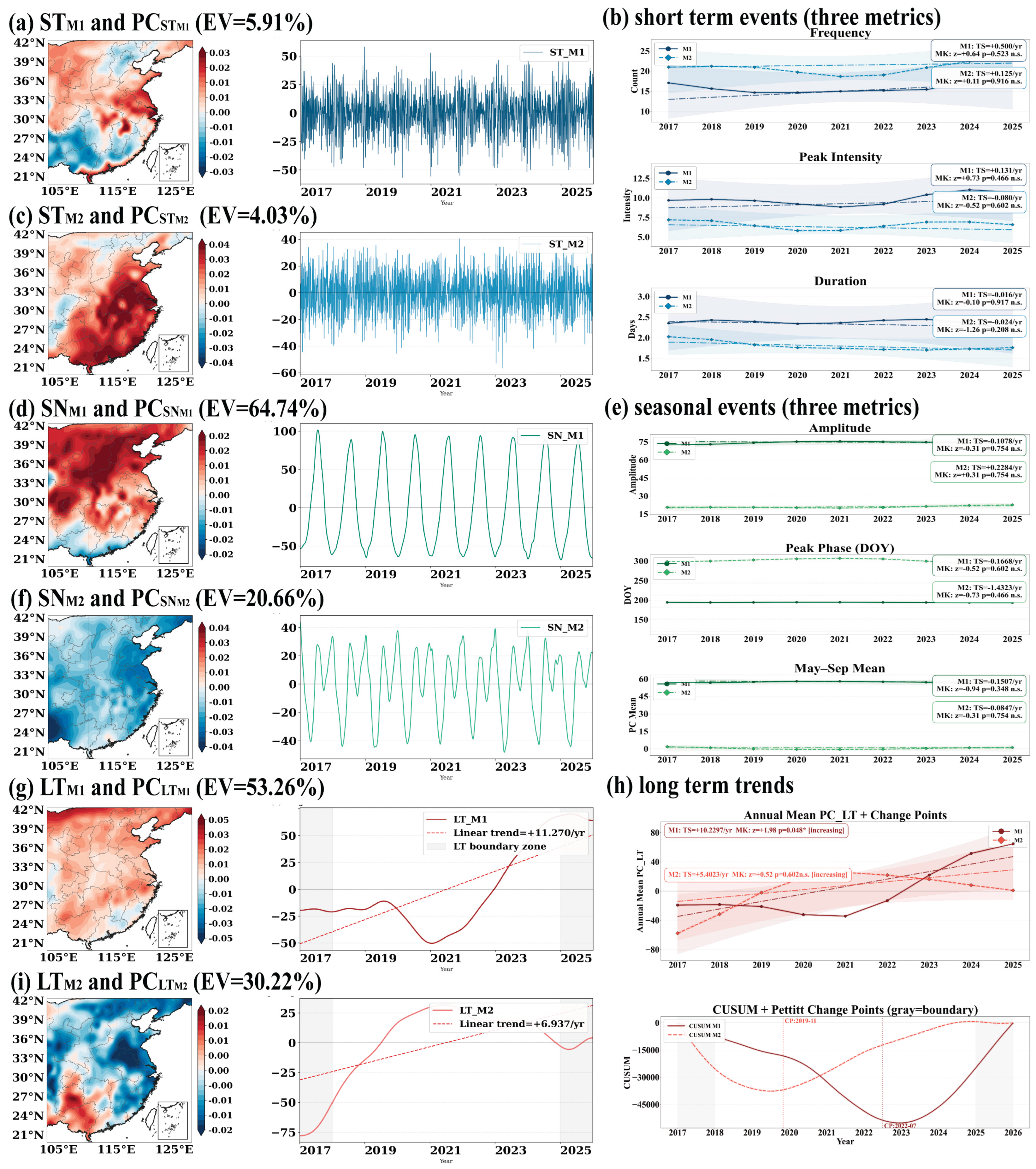
Figure 2.
SHAP ranking of influential factors behind each mode with PINN serving as soft constraints.
Figure 2.
SHAP ranking of influential factors behind each mode with PINN serving as soft constraints.
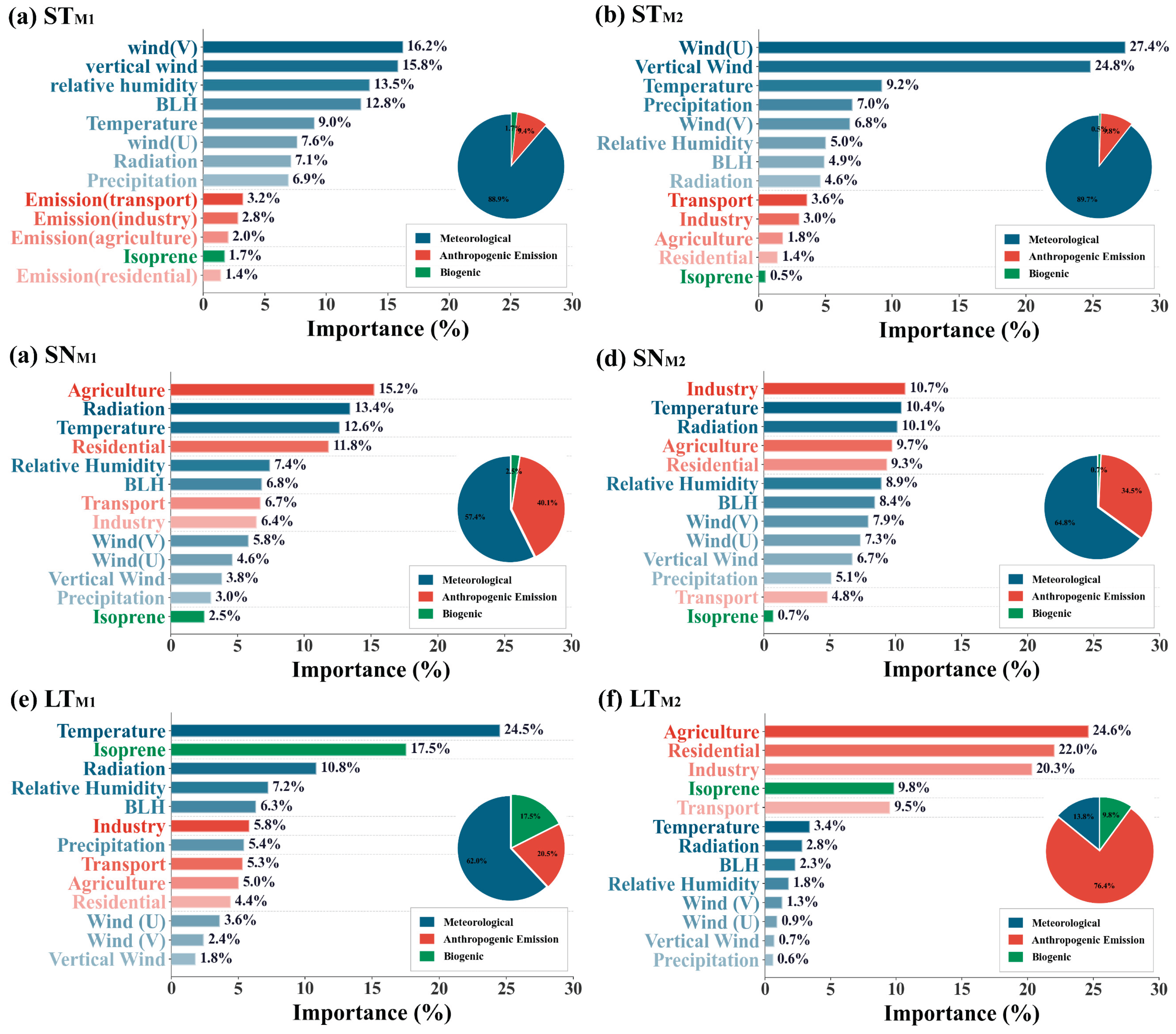

Table 2.
Rolling variation characteristics of 12 cross-scale response relationship pairs (β).
| Task | Ralations | Slope β | P | Mean β | MK z | R2 |
|---|---|---|---|---|---|---|
| A | SN_M1>ST_M1 | -0.002 | 0.3 | 0 | 6.71 | 0.58 |
| A | SN_M1>ST_M2 | -0.004 | 0.22 | 0 | -13.69 | 0.72 |
| A | SN_M2>ST_M1 | 0.323 | 0 | 0.02 | -2.79 | 0.66 |
| A | SN_M2>ST_M2 | 0.003 | 0.54 | -0.02 | 11.63 | 0.76 |
| A | LT_M1>ST_M1 | -0.053 | 0 | -0.03 | -9.92 | 0.88 |
| A | LT_M1>ST_M2 | 0.252 | 0 | -0.23 | 13.06 | 0.86 |
| A | LT_M2>ST_M1 | -0.411 | 0.85 | -0.97 | -0.18 | 0.88 |
| A | LT_M2>ST_M2 | 0.087 | 0.21 | -0.29 | -1.22 | 0.86 |
| B | LT_M1>SN_M1 | -2.819 | 0 | 15.17 | -13.76 | 0.96 |
| B | LT_M1>SN_M2 | 2.976 | 0 | -1.36 | 23.48 | 0.97 |
| B | LT_M2>SN_M1 | 0.548 | 0 | -8.84 | 8.07 | 0.99 |
| B | LT_M2>SN_M2 | 4.285 | 0 | 10.15 | 9.5 | 0.99 |
Disclaimer/Publisher’s Note: The statements, opinions and data contained in all publications are solely those of the individual author(s) and contributor(s) and not of MDPI and/or the editor(s). MDPI and/or the editor(s) disclaim responsibility for any injury to people or property resulting from any ideas, methods, instructions or products referred to in the content. |
© 2026 by the authors. Licensee MDPI, Basel, Switzerland. This article is an open access article distributed under the terms and conditions of the Creative Commons Attribution (CC BY) license (http://creativecommons.org/licenses/by/4.0/).
Copyright: This open access article is published under a Creative Commons CC BY 4.0 license, which permit the free download, distribution, and reuse, provided that the author and preprint are cited in any reuse.