

Submitted:
05 October 2026
Posted:
08 October 2026
You are already at the latest version
Abstract
Whether observation dynamics can leave distinct matter records under identical physical initial conditions and subsequent external forcing depends on three questions: whether observation initial states have a well-defined identity, whether they can be prepared, and whether their evolution satisfies the common field equations. We construct a local realization within the existing five-dimensional response space and quadratic common action of PODA. With spatial and temporal references fixed, primitive response transport yields nonzero mixed curvature and identifies the observation coordinate through distinguishable comparison records; the image of its field data is an invariant subspace of the transverse dynamics. The field restoring force and a nonzero current overlap allow a single matter input to prepare arbitrary sufficiently small joint initial states. An explicit eighth-degree polynomial protocol carries the state initially at rest to two final states with identical matter position, matter velocity, and observation configuration, but opposite observation velocities. The input vanishes continuously at both endpoints, and the net work equals the stored energy. After release, the two-frequency displacement and the observation comparison probability obey a common integral identity. We also derive propagation relations for initial-state mismatch, finite readout precision, and control-waveform errors, and retain the complete calculations for matter sources, the one-loop relativistic response, and indirect tests involving common parameters. The result is an existence theorem for preparation and response in the specified local realization, within the stated quadratic dynamics and external matter-source model.
Keywords:
PODA
; observation state
; common action
; mixed curvature
; finite-time preparation
; matter response
1. Introduction
A release experiment usually begins by specifying position, velocity, and external fields. Different preparation histories should lead to the same subsequent motion whenever these initial data agree at release. This expectation contains an assumption: the recorded initial data encompass every state variable that determines the motion. If another variable participates in the joint evolution without being recorded in these matter initial data, identical positions and velocities may lead to different trajectories. Establishing the physical significance of such a difference requires identifying the omitted variable, explaining how it is prepared, and specifying how it can be distinguished independently.
PODA addresses this question through a joint structure of physical states and observation-formation states. M–L–O provides the structural background relating laws, conditions, and observational restrictions; the set-theoretic and categorical foundations identify observation states through complete behavior and specify, through the admissible domain, how the two kinds of state may be paired [1,2,3,4]. An observation state is therefore not another name for an instrument setting. Whether two modes of formation represent the same observation state depends on their distinguishability under the declared complete comparisons. Instruments participate in preparation and recording through matter couplings, while their own dynamics remain subject to the common action.
The foundational structure distinguishes physical states from observation states; a particular realization must supply its response functions. The phase-transport and common-action formulations connect coherent comparisons, response geometry, and joint dynamics [5,6]. Here we construct the map from primitive variations to field initial data and establish its compatibility with parent-field evolution for a specified local realization. This leads to a definite existence problem: can a single realization connect observation identity, the actual response map, and the common equations of motion to a preparation procedure using only matter input, and then predict release records that have not already been used for calibration?
We give a local affirmative example. The internal representation, generator, and field action are taken from the existing theory. The additional specifications are a local admissible domain, position-resolved response transport, and an external source acting on the retained matter coordinate. This transport both gives the observation coordinate distinguishable behavior and maps it to a transverse field mode satisfying the Gauss constraint. Pulling back the same action retains the field inertia, restoring force, and feedback on matter. The resulting finite-time preparation pulse returns matter to identical initial data while leaving opposite observation velocities. The subsequent matter motion and primitive comparison records are then determined by the same parameters.
Controllability, observability, and Gramian methods for finite-dimensional linear systems are well established [7]. Input–output realization and structural identifiability further distinguish recovery of a state model from uniqueness of its internal parameters [8,9]. These methods are used here to determine whether a system derived from the PODA common action admits the required preparation while preserving observation identity and the physical projection. The contribution is a complete construction from behavioral comparison to a constrained field-data image, explicit preparation, and joint records. We also show that data on a reference section alone do not uniquely determine the required mixed curvature. The existence construction and a uniqueness claim therefore have distinct mathematical content.
The paper follows this preparation problem. Section 2 specifies observation identity and the response realization; Section 3 treats the constraints and establishes dynamical compatibility; Section 4 and Section 5 derive finite-time preparation and release records, respectively; and Section 6 examines independent comparisons, errors, and experimental criteria. Numerical results are presented in Section 7. The appendices retain the derivations of the general forced response, matter sources, multimode feedback, relativistic kernels, and low-energy indirect tests, so that the conditions of applicability can be traced through the equations.
1.1. Physical Projection and Scope of Comparison
The physical projection is fixed before the construction begins: it records the retained matter data and the spatial and temporal references. The dynamical matter data held fixed between the two releases are ; motion during preparation and the actuator states may differ. If a different task includes all Cauchy data of the parent connection among its physical initial data, the two final states constructed here no longer share that enlarged set of initial data. This distinction is determined by the comparison task and cannot be removed by reclassifying states after observing the response.
The local realization uses a closed quadratic internal channel, positive matter inertia, and a current profile aligned with the selected transverse mode. The preparation term is specified as , whose direct variation with respect to the observation coordinate vanishes. The vectors, effects, and comparison paths entering the coherent response belong to the declared comparison data of this realization. These data are inputs to the existence theorem; their experimental meaning and higher-order limits are discussed in the main text and appendices. The probability readout uses the prescribed Hermitian pairing and does not rederive the Born rule.

Table 1.
Data used in the existence theorem and their roles.
| Data | Role in the proof |
|---|---|
| Physical projection and admissible domain | Define identical matter initial data and the observation variations that may be compared. |
| Complete transport and response spectrum | Determine observation identity, the connection, the projector, and the primitive field-data map. |
| Quadratic channel and boundary conditions | Ensure constraint propagation, mode invariance, and dynamical compatibility of the pulled-back equations. |
| Current overlap and external matter source | Produce feedback on matter and enable finite-time preparation. |
| Two independent records | Test the joint prediction without repeatedly defining the tested quantities from a single trajectory. |
2. Observation Identity and a Local Response Realization
Observation states must be defined before field coordinates are named. We first specify the meaning of complete comparison on the local admissible domain and then construct the induced transport. All response data needed for the construction are given in this section; the subsequent dynamical analysis uses these data and the existing action.
2.1. From Observation Identity to a Specific Response
The set-theoretic and categorical foundations first establish the identity of observation states. Two primitive formation labels belong to the same observation state if they have identical outcomes and realizability in every declared comparison. Realizability is retained in the joint admissible domain . Observation variations at fixed physical state must therefore remain within the actual fiber ; labels cannot be recombined arbitrarily under the assumption that the new pair is also realizable [2,3]. This gives s a definite theoretical meaning without requiring an interpretation as an instrument control.
The bijection between observation states and complete realized behavior families in the categorical formulation likewise concerns the actual behavior family. It removes redundant representations while retaining all distinguishable behavior, but does not automatically include field modes that have not been specified. Uniqueness of observation identity and reachability of a particular transverse field initial state are thus successive propositions requiring separate proofs.
Coherent comparison supplies a route from observation identity to response transport. A nonzero vector response permits comparison of its normalized rays. The geometry of phase transport was established by Berry and Simon, with Wilczek and Zee extending the construction to non-Abelian subspace transport [10,11,12]. Matrix responses can also be separated into a positive amplitude and a unitary polar factor [13]; a rule for comparing different fibers must still be supplied. In the scalar PODA construction, a smooth nonzero response determines its phase connection [5]. A specific response or complete transport remains an input: final field data alone cannot determine a unique primitive variation. Both vector responses and spectral subspaces can produce curvature; the particular mixed component needed here must be computed from the actual derivatives of the prescribed response.
The common-action formulation uses complete transport to determine the parent connection and an isolated spectral cluster of the response operator to determine the projector. Pulling both objects back to spacetime then defines the common action [6]. That work distinguishes independent parent-field variations from composite variations in primitive variables: the latter give chain-rule Euler equations, and recovery of all independent parent-field equations requires the corresponding variational completeness. Whether admissible parent-field initial data arise from primitive observation directions at fixed physical projection must therefore be decided by the response map.
Table 2.
Foundational results used here and the response data required for their realization.
| Source | Foundational result | Input required for a specific realization |
|---|---|---|
| Set-theoretic and categorical foundations | Behavioral identity of observation, admissible domain, minimal realization, and unique descent | The actual admissible fiber at fixed x and its realizable variations |
| Phase and subspace transport | Phase comparison, line-bundle holonomy, and non-Abelian subspace transport | The response function or complete path transport for the internal channel |
| Common-action formulation | Spectral projector, common action, parent-field equations, and recovered models | A realization on the original joint domain and its derivatives in observation directions |
| Primitive realization developed here | Relation between primitive variations and field data, constraints, and preparation criteria | for the selected direction and the actual admissible initial data |
2.2. Position-Resolved Physical States and the Admissible Domain
We first specify the physical states. Let the local state of the original matter sector be realized as a state bundle with fixed spatial and temporal labels, where U is the spacetime region identified by those labels. The fibers retain the original matter states and their source data. Let be a regular patch of this bundle, and let read out position and time. An actual matter configuration is a section , so that
contains matter states and is not spacetime. The projection ℓ reads position and time, whereas its fibers carry the matter states. The coordinate used below changes only the fiber data, so Eq. (1) holds throughout preparation and release. This reference is prescribed independently of the observation coordinate and bridge field and introduces no propagating degree of freedom. A constant displacement of an unlabeled homogeneous flow does not have the same readout meaning; the relevant conditions are discussed in Appendix C.
Choose a real transverse spatial eigenmode with unit norm, zero divergence, and , and define
On we use , suppressing this pullback in what follows. Take the existing five-dimensional response bundle, a nonzero anti-Hermitian bridge generator K with , and a reference response with two spectral blocks. Define
Here is the rank-three projector of the existing three-plus-two spectral decomposition, and . Both and complete transport are prescribed response data; the other retained vacuum responses remain at their reference values. K carries no additional adjustable coupling, and the spatial profile is the prescribed . This specification completes the dependence of the response on the primitive observation coordinate without changing the common action.
2.3. Identification of the Observation Coordinate by Complete Comparison
For a path in this local admissible domain, prescribe the complete response transport as
It preserves the Hermitian pairing and satisfies composition, reversal, smoothness, and thin-homotopy invariance, placing it within the reversible comparison transport used in the unified formulation [6,14]. We use the parallel-transport convention . The infinitesimal connection recovered from Eq. (4) is precisely Eq. (3).
We must also establish that survives the quotient by complete behavior. Include the following vectors, effects, and path comparisons in the admissible comparison family of this realization. For the original profile , start at the same physical-state point , at a location where , choose a fixed reference path in the y direction, and set . Choose the channel orientation . Then
In the neighborhood , this record is strictly monotone in the observation coordinate. Distinct values of are distinguished by at least this admissible comparison and therefore cannot be identified in the complete behavioral quotient. This realizes the set-theoretic and categorical notion of observation identity [2,3] and supplies a behavioral basis for using as a local coordinate of the observation state.
The distinguishability proof assumes that the comparison in Eq. (5) belongs to the admissible family. Actual sampling further requires the corresponding preparation, effect, and matter reference. The probability pairing is prescribed as part of the response realization; the test vector defines the comparison and is not introduced as a new particle in the release equations.
Throughout, we take , hence , together with and . This convention fixes the orientations of both the current and the comparison transport. With , the comparison vector is , giving the signs in Eq. (5) and in all subsequent probability, preparation, and release results.
Since the same generator is used throughout, , and the curvature is
Where , the mixed curvature between observation and physical directions is nonzero. With and complete transport preserved, the connection cannot descend to one depending on X alone. This geometric distinction agrees with the behavioral distinction established above.
3. Common Action, the Gauss Constraint, and Dynamical Compatibility
Appendix F shows that the same reference section admits different mixed curvatures. Section 2 specifies one such response extension. The response realization determines the origin of the field data, while the common action determines their evolution. The two must remain compatible throughout the history. As in constrained Hamiltonian reduction [15,16], the admissible initial data must be separated from variables fixed by the constraint equations. We first eliminate the nondynamical temporal component and derive the mode coefficients. We then substitute the primitive response of Section 2 into the complete quadratic field equations and check the equations outside the retained mode.
3.1. Field Action and Conserved Matter Current
The common-action realization supplies the gauge-invariant quadratic field channel used below [6]. To distinguish the coefficients, we denote its inertial weight by , its orbit coefficient by , and the observation inertia along the path by . The original field action is
The metric signature is . is the invariant formed from the original connection and the collective direction; the direction coordinate introduces no independent particle. We retain the stated quadratic-order conditions of this channel and the original definition of the matter source, .
Choose an admissible collective mode of the original matter sector. Suppose that its reduced kinetic energy, potential, and linear current have the form
where the spatial profile is determined by the current matrix element of that matter mode. Then holds identically. This is a linear form of a conserved current generated by displacement, with the continuity equation guaranteed by definition. Conservation alone, however, does not establish the physical origin of the source: the existence of and the matter mode carrying it must still be calculated from the coupling in the original . Whether ordinary charge can source this channel depends on that same coupling structure.
We vary x and the field together, retaining the field’s feedback on matter. During preparation, a calibrated physical generalized force may be applied through the term in the reduced action. Its work is retained in the energy equation. The preparation in Section 4 uses only this physical input.
3.2. Elimination of the Gauss Constraint
Take a real spatial mode , normalized by , and write
The spatial pairing and integration by parts use the same periodic boundary conditions, or prescribed boundary conditions under which the boundary terms vanish. The original temporal-component equation gives
The Gauss constraint determines the temporal component, which varies with both x and . Substitution into the original action yields
Define , , and . Writing as gives
with all coefficients determined by the same restriction:
Constraint elimination and restriction of the action give these coefficients; the spatial field equations remain to be checked. This check can be completed for the following two classes of eigenmode.
3.3. Transverse Mode: The Curvature Term from the Original Current Coupling
If
then , and
The full spatial field equation and matter equation become, respectively,
Thus, within this quadratic field channel, the residual in every orthogonal spatial direction vanishes, and the Gauss constraint is also satisfied. The mode restoring coefficient is determined by the original field-gradient and mass terms. It preserves the mode’s own dynamics, so this branch cannot be replaced directly by a free solution with constant potential.
The term linear in velocity comes from the original , whose spatial integral is . On the joint path it gives the one-form and curvature
This curvature lives on the reduced configuration space , and its coefficient is the current–field-mode overlap . It is not a tensor component on the same domain as , which lives on the primitive response domain. The latter supplies the field response through Eq. (6) and the pullback map; the former arises from the spatially integrated matter coupling . In particular, with the position reference fixed, a pointwise curvature in a matter-fiber direction cannot be identified directly with the integrated overlap . The response realization and common action relate the two curvatures, while their coefficients also depend on the matter mode carrying the current.
3.4. Longitudinal Mode: Three Linked Constraint Corrections
The same Gauss constraint changes the longitudinal inertia, the mixed-curvature coefficient, and the matter stiffness. These three corrections are linked; retaining all of them makes the reduced equations consistent with the original field equations.
The result can also be checked directly by varying the source. The generalized force on x from the original source is
The matter equation is therefore . The spatial field equation reduces to . The temporal-component constraint, continuity equation, and full spatial equation all agree with the same reduction.
3.5. The Field-Data Image of the Primitive Response
Take the observation section . Since each matter configuration is a section of the fixed state bundle, matter motion does not alter the pullback of the position reference. The spacetime field data of the primitive response are therefore
Here is the component, along the selected generator, of the curvature contraction in the observation direction, and is determined by the covariant variation of the projected subspace along that direction; the general definitions appear in Appendix F. Equation (6) and the constant projector give these values directly. The variation direction lies in , while complete comparison preserves its identity as an observation direction. Thus q is the amplitude of the primitive observation coordinate on this section.
Substituting Eq. (20) into the existing quadratic common action again gives
The term obtained by integration by parts gives the same Euler equations as the original current term , with the endpoint conditions already specified. Varying together yields
Both the observation kinetic energy and its restoring force are inherited from the original field terms; no independent law of motion has been appended for the observation coordinate.
In this realization, the equations of the pulled-back action also satisfy the parent-field equations. We verify below that the field-momentum equation, matter current, Gauss constraint, and retained transverse mode form a quadratic invariant subspace. Since Eq. (20) is itself supplied by the primitive response, the same calculation establishes
The positive inertias make the quadratic initial-value problem regular. Sufficiently small initial states and preparation pulses remain within the local admissible domain. This conclusion concerns the quadratic channel; the scope of the full nonlinear field theory and quantum response is discussed in Section 8.
3.6. Compatibility of the Transverse Field-Data Image with Evolution
Write for the same observation amplitude and take and , retaining the matter inertia m, stiffness , and current overlap f. Consistently with Eq. (26), denotes matter stiffness and k denotes only the spatial wavenumber. In the existing quadratic channel, the first-order field and matter equations are
The Gauss constraint has already been eliminated, and the continuity equation for this transverse source holds identically. Substituting Eq. (23), the right-hand side remains in the same spatial mode and uniquely determines
Proposition
(Dynamical compatibility of the selected transverse image). Within the existing closed quadratic channel and under the boundary conditions above, the image of Eq. (23) is invariant under the common field evolution. Equation (25), obtained by pulling back the same action, is compatible with the parent-field evolution on that image.
Proof.
The right-hand side of the field-momentum equation is , and that of the field-coordinate equation is ; neither has a component in any orthogonal spatial direction. The normalized spatial integral gives the second row of Eq. (25) directly from the matter equation. The constraint divergence remains zero under evolution. Comparing these four components with gives the compatibility identity. Uniqueness of the constant-coefficient initial-value problem then establishes correspondence throughout the evolution. □
The proof also explains why substitution into the action alone is insufficient: compatibility requires the discarded equations to have zero residual, in addition to the retained equations being satisfied. The verification concerns the quadratic internal channel already assumed closed in the original formulation and its transverse spatial mode. Nonlinear equations for other internal fields, relative directions, and the metric lie outside this quadratic proposition. Near a static vacuum with no current, backreaction such as field stress may first appear at higher order in amplitude; vanishing linear residuals do not justify discarding it. The restrictions concerning open continua and quantum errors in Appendix D also remain in force.
4. Finite-Time Preparation by Matter Input
Once a compatible field-data image has been established, preparation becomes a definite boundary-value problem: can a force acting only on matter return its position and velocity to their initial values in finite time while leaving a prescribed velocity in the observation coordinate? We first determine the reachable states through a controllability criterion, then construct a pulse that vanishes continuously at both endpoints.
4.1. The Restoring Force Enables Finite-Time Preparation
Write the reduced coefficients as , and continue to denote the matter stiffness by . The system is
Both the transverse and longitudinal branches have . Allow only the physical force u as input and record only . With , we have
The four-dimensional state consists of two coordinates and their velocities, giving a first-order representation of the second-order joint equations. Its dimension counts the dynamical variables retained here and imposes no further restriction on the dimension of the primitive observation space.
Proposition
(Modal preparation and readout with one physical input). For the constant-coefficient realization in Eq. (27), suppose that , , and . The single physical input u makes the system controllable, and the complete matter record makes the initial state of the calibrated model observable. The conclusion does not require .
Proof.
Form the controllability matrix and the observability matrix . Direct calculation gives
Both determinants are nonzero, so both matrices have rank four. By the controllability and observability criteria for linear systems [7], the reachable space is spanned by , and the unobservable initial-state subspace is . The nonzero determinants make the reachable space the full state space and the unobservable subspace trivial. □
These rank tests apply to the stated linear realization. For nonlinear systems, the corresponding questions of accessibility and state distinguishability involve the system vector fields and observation functions [17]. No nonlinear rank condition is needed for the constant-coefficient model considered here.
Controllability permits the following preparation. The external force first moves the matter coordinate x, transferring work to the field mode through the original coupling, and then returns it to a prescribed position and velocity at the preparation endpoint. After the force is switched off, the matter responses to different modal initial states can be compared. The retained matter data are held fixed in this comparison, while the field initial data may differ. Matter motion during preparation is precisely how this difference is produced.
The constant-potential limit reveals the role of the restoring force. If and , then
This conserved quantity restricts what the sole input u can achieve: starting from the same initial state, fixing the target x prevents arbitrary changes in . At the same time, a constant is absent from the matter record. Both the controllability and observability matrices consequently have rank three. The positive restoring coefficient inherited from the common field channel removes this obstruction. It also explains why the preparation theorem depends on the field restoring force and does not apply directly to the constant-potential model of Appendix A.
4.2. A Gramian Preparation Protocol
Let the preparation interval be , with known initial state and target . Define
By Proposition 4.1, every gives . Substituting the control
into the state-transition formula yields . An orthogonal decomposition of any control reaching the same target gives
with equality for Eq. (31). This minimum measures the squared-integral input cost. The physical energy, determined by the action, is
A very short preparation time or a very small current overlap increases the control cost and required peak force. The mathematical conclusion for every allows square-integrable inputs without an amplitude bound. Practical use is also constrained by the peak input, bandwidth, spatial profile, propagation delay, and validity of the local approximation. In the linear model, reducing the target amplitude reduces the control by the same factor, but also reduces the measurable signal.
For example, choose the two targets . Under the same post-release external protocol , they have identical matter positions and velocities and identical spatial field-mode amplitudes , but different field momenta. They satisfy
If instead is held fixed and differs, the same matter initial data give . These two comparisons read, respectively, momentum and position differences in the observation channel. In the longitudinal branch, the Gauss constraint also makes depend on . The comparison therefore holds the spatial field-mode amplitude fixed, while the temporal component changes with the prepared momentum difference.
4.3. An Explicit Matter Pulse Vanishing Continuously at Both Endpoints
We now realize controllability through a finite pulse that can be substituted directly into the equations. Take the preparation interval , start with every coordinate at rest, and require the endpoint at to satisfy
Set and introduce the dimensionless combinations
The second joint equation gives directly
To satisfy the initial and final matter conditions in Eq. (35) and make the input vanish continuously at both endpoints, impose
The integral condition has a direct meaning: the accumulated action of the observation restoring force during preparation allows the matter displacement to return to zero while the observation velocity retains the value w. For , this condition ceases to be defined, and the constant-potential conservation obstruction derived above returns.
An eighth-degree polynomial satisfying all the conditions is
The coefficient matrix of the five endpoint and integral conditions has determinant , so the solution is unique within this polynomial family. This does not imply uniqueness among all admissible preparation protocols, nor does it establish minimum energy expenditure or minimum peak force.
Substituting Eq. (37) into the first joint equation determines the sole required external input:
Set outside this interval. Equation (38) gives ; for fixed , the input and its one-sided rates of change are finite. The observation equation has no applied source at any time. The input u first drives matter, which transfers energy to the observation mode through the original coupling and returns to the same matter initial data before release.
Replacing w by reverses the entire preparation input and trajectory, giving the final state . Both observation configurations have equal to zero, but the velocities in their dynamical initial states differ. With release time , both preparations are followed by the same protocol ; their different internal currents arise from their respective joint evolutions.
4.4. An Existence Theorem for Preparation and Response
Theorem
(Primitive observation preparation and matter response in this realization). Consider the position-resolved response realization specified by Eqs. (1)–(4), the closed quadratic channel of Section 3, and the external source . Assume , , and . For every fixed and sufficiently small , the two signs of Eq. (40) give two joint preparations satisfying the model equations and remaining in the admissible domain. At release they have identical matter positions, matter velocities, and observation configurations, with observation velocities . Both satisfy the Gauss constraint, are compatible with parent-field evolution, and produce
Here are given by Eq. (45). The net preparation work is the same in both cases, equal to .
Proof.
Equation (5) first ensures that the observation coordinate remains distinguishable in the complete behavioral quotient. Equation (20) gives its actual field-data image, whose transversality makes the Gauss constraint hold identically. Substitution of the polynomial boundary values into Eq. (37) gives Eq. (35); Eq. (40) and both joint equations are satisfied simultaneously. The primitive dynamics follow from Eq. (21), and Eq. (23) preserves the correspondence throughout release. Uniqueness of the initial-value problem identifies the release solution with that given in Section 5. Finally, the joint energy satisfies . Its initial value is zero and its final value is , so the net work equals this value. □
The theorem establishes the existence of preparation in this local realization. The two releases hold the declared matter initial data and physical references fixed. Actuator states are not among the fixed data, and the preparation process allows matter motion and energy exchange. The construction simultaneously preserves the physical projection along observation directions, reaches the target final states through matter input, and begins release from identical retained matter initial data.
4.5. Bandwidth and Local Validity of the Finite Pulse
The input is continuous on the full real time axis, polynomial within the preparation interval, and has finite one-sided derivatives at the endpoints. In general, it is neither continuously differentiable everywhere nor strictly bandlimited. Let . Using and integrating by parts twice yields
Finite duration and finite peak amplitude therefore do not ensure that the excitation remains strictly within a low-frequency interval. If the actuator transfer function or filtering changes the input to , the change in the prepared final state is
Both the norm and the Gramian here use a prescribed dimensionless state scaling. Equation (43) is an operator bound within the same linear system; it does not estimate departures of the actual out-of-band dynamics from the quadratic model.
For fixed T, the preparation trajectory and input scale linearly with . On any prescribed finite release interval, the corresponding solution also depends continuously and linearly on . A sufficiently small amplitude therefore keeps the entire history within the local admissible domain and the monotone comparison branch. Reducing the amplitude also reduces the difference between the records, so experimental design must weigh this condition against resolution.
5. Release Dynamics from Identical Initial Matter Data
After preparation, the external source is switched off in both runs, and release time is denoted by . We first obtain the full release history and then relate it to the primitive comparison record. Although the two initial accelerations already differ, the complete time record provides a stronger test by constraining the frequencies, phases, and relative amplitudes together.
5.1. Paired Initial States and the Complete Release Solution
Within the quadratic field reduction of Section 3, choose any sufficiently small real amplitude and compare
These are admissible field initial data with identical initial matter positions and velocities and identical initial field configurations, but opposite canonical field momenta. Their total initial energies are also equal, both being . After release, both runs have the same external source, . The internal current can subsequently differ because the motions differ; this is a consequence of the joint evolution, rather than a difference in the external sources applied after release. The response realization in Section 2 and the pulses in Section 4 give both initial states an explicit origin in primitive observation data.
To obtain the complete displacement record, define
For , , and , both squared frequencies are nonnegative and ; when , the solution is understood in the continuous limit . Eliminating gives
The initial conditions are , , and . The difference between the two records is therefore
For the positive initial sign, the field amplitude is
At zero frequency, is interpreted as t. Substitution into the two second-order equations verifies both the initial data and the feedback, without prescribing an additional matter force.
The same calculation yields an early-time criterion that distinguishes the complete equations from the equations with the restoring term omitted:
The two calculations predict the same initial acceleration, but their displacements first differ at order . Agreement of initial accelerations alone is therefore insufficient to establish the correspondence between the path and field descriptions.
An experimental comparison can follow the preparation protocol above: apply the two preparation inputs, return the matter to the same position and velocity at release, and record the subsequent motions under the same external source. Once the primitive mapping and matter calibration have been established, Eq. (47) jointly fixes the sign reversal, the two frequencies, and their relative amplitudes. These quantities must be predicted from independently calibrated coefficients, without refitting each release curve. In practice, fitting the complete two-frequency record is preferable to estimating a fourth derivative from noisy displacement data; the fourth-derivative relation is more useful as a theoretical diagnostic. The attainable preparation amplitude and energy, higher-order corrections, and readout errors remain subject to the conditions discussed above.
6. Joint Records and Their Tests
The matter trajectory shows how the observation initial state enters the feedback equations, while the comparison record independently identifies the prepared observation state. Their relationship provides a joint test only when the two records are obtained independently.
6.1. Joint Predictions for Observation Comparisons and Matter Records
The realization also relates the primitive comparison record directly to the matter response. For the two releases following opposite preparations, the linear joint equations imply . Reading Eq. (5) along the same calibrated comparison path gives
On the same inverse branch, , integration of the matter difference equation yields
The right-hand side is obtained from the primitive observation comparison, and the left-hand side from the matter motion. Their normalizations, the coefficients , and the path integral must be calibrated independently and held fixed across releases. Equation (51) requires only an integral of displacement and a velocity record, making it more suitable for a consistency test on measured data than a comparison of high-order derivatives. At the initial instant, the records must also satisfy
The experimental sequence is thus specified: calibrate the observation comparison along a common reference path, apply the two pulses , verify the matter initial data and the vanishing input at release, and then record the matter motion and the corresponding comparison response. The inverse relation, the two-frequency release solution, and the energy balance constrain the results jointly. Comparison-readout backaction must be controlled within the same realization, or assessed by repeated preparations with readout at different times; the ideal record formula does not itself supply a detector design.
The term in the action explicitly denotes an external matter source: its variation with respect to x is u, whereas its variation with respect to q vanishes. If an apparatus also drives the parent field directly, the associated source term must be retained, and the single-input formulas of this section no longer apply. In particular, identifying u with an applied electric field in the K direction while omitting its contribution to the field equation changes the problem being solved. Appendices Appendix C–Appendix E discuss selective forces, continuous spectra, and high-energy benchmarks; experimental accessibility depends on the actual parameters and control couplings.
6.2. Imperfectly Opposite Preparations and the Integral Test
Exactly opposite preparations make the result transparent, but experimental analysis need not require perfectly opposite terminal states. Provided each record remains on the same branch , the comparison probabilities can be inverted separately:
Integrating the common matter equation gives the more general identity
A terminal velocity mismatch, an initial observation displacement determined by comparison, and a residual external force each contribute a separately measurable correction. Equation (51) is the special case of identical matter initial data, zero residual source, and opposite observation initial states.
For the ideal difference inversion, suppose both the true and the perturbed values lie within . The derivative of the inverse sine and the mean value theorem then bound the probability error on the right-hand side by
If the two comparison records contain independent Bernoulli trials, respectively, then
This variance includes only independent sampling noise. Common drift, correlations between preparations, and calibration errors require covariance contributions and do not automatically disappear as the number of repetitions increases. Equation (55) also shows that errors are amplified near the ends of the inverse branch, so the path and amplitude should be chosen with a definite margin.
If the actual matter equation contains an unaccounted differential force , the right-hand side of Eq. (54) acquires the term . Omitted modes, readout backaction, and higher-order terms can therefore be represented by the same residual. A persistent discrepancy can exclude the selected realization only after these contributions and the experimental errors have been controlled.
6.3. Correction for a Finite Comparison Time
Equation (5) is a response functional on an equal-time section. It does not assume that an experiment can transmit a record instantaneously along a spacelike path. If the actual comparison follows a path with a finite temporal extent, transport remains exactly expressible because the channel contains only one fixed generator:
The probability formula then uses in place of q. Suppose the time along the path differs from the assigned readout time by at most , and over that interval. Writing , one obtains
The adequacy of the equal-time approximation can thus be checked against the actual path and dynamical range. When the comparison time is appreciable, the calibrated path kernel must be applied to the theoretical trajectory before comparison with the record; a time average cannot be inserted directly into the instantaneous integral identity. This correction addresses only the finite comparison time in the specified channel. Actuator and detector backaction must still be retained separately.
6.4. Independent Records and Discrimination Between Models
The comparison probability must be obtained through an independent comparison. If is first reconstructed from using the matter equation and then substituted into , the resulting integral identity merely restates that equation. Reconstruction from a matter time record can estimate the state of a calibrated model, but it cannot also provide independent evidence for that model. A valid test should establish the comparison path, response pairing, and matter parameters separately, then compare predictions against held-out preparation amplitudes, pulse durations, or release records.
Before the comparison, the preparation endpoint, residual external source, and readout bandwidth must also be recorded. If continuous readout perturbs the system appreciably, its backaction must enter the common equations. For reproducible preparations, different readout times may instead be assigned to different runs, with the consistency of the preparation distribution verified. These procedures obtain the quantities in Eq. (54); they do not identify apparatus settings directly with primitive observation states.
Even if the joint records satisfy every formula, these effective equations alone cannot exclude all conventional coupled-oscillator or field models. Any model retaining the same states, couplings, and readout map produces the same records. The additional content open to verification in this PODA construction is the correspondence between the quotient by observational behavior, the fixed physical projection, and the field data, together with the restrictions that this correspondence places on admissible comparisons. Discriminating between theories requires determining whether they admit the same states and parameter relations for the same preparation and readout task. Similarity between two curves is insufficient for that purpose.
7. Numerical Results and Reproducible Calculations
The analytical proofs do not depend on numerical sampling. Computation is used here to verify the polynomial construction, field constraints, and energy balance, to compare two independent solution methods, and to display the scale of the joint records. Except for the explicitly identified high-energy benchmarks, the figures use dimensionless synthetic parameters and do not represent completed experiments.
7.1. Verification of the Complete Preparation, Energy Balance, and Release
Choose the synthetic coefficients , , , , and , with and . Then and . The required pulse is finite in duration, with a peak of approximately and exactly zero values at both endpoints. The peak matter speed is approximately , and the peak observation amplitude is approximately . All amplitudes scale linearly with , and the energy scales with , so the trajectory can be reduced to the range required by the local approximation at fixed T.
The polynomial coefficients, endpoint conditions, joint-equation residuals, and net work are verified using rational arithmetic. An independent integration of the ordinary differential equations gives a terminal-state error below and a preparation-trajectory error below ; the subsequent release displacement difference agrees with the analytical prediction to within . These errors verify the implementation of the stated equations; they do not estimate higher-order corrections to the underlying theory.
The net preparation work is , equal to the target initial-state energy. The cumulative positive and negative work during the pulse is approximately and , respectively. The actuator both supplies and absorbs energy during preparation, so its required capacity cannot be assessed from the net work alone. Figure 1 shows the complete process, and Figure 2 relates the observation comparison to the matter record.
8. Matter Realizations and Range of Applicability
8.1. From an Admissible External Source to a Specific Matter Coupling
The existence theorem uses the external matter source . Although this input is well defined in the stated variational problem, a specific matter action is still needed to explain how an experiment supplies it. Appendix C calculates the bridge current from the Dirac fundamental representation already present in the unified-action paper, constructs two counterflows, and derives the relation tying inertia and coupling to the same density. A common external force drives only the common displacement of the two flows; the relative motion required for preparation is driven by a difference between forces selective to the internal states. Without position markers, the accessible record is a relative velocity or weighted current. A constant displacement of a uniform flow cannot simply be treated as a position record.
This matter example shows how a nonzero overlap arises and why realizing an effective external source requires more than a choice of notation. If the control couples directly to the bridge field, the associated source enters the field equation and the input map must be recalculated. The existence theorem for a prescribed does not establish a complete actuator and detector within the original Dirac matter sector. The appendix retains the force difference, current normalization, and multimode feedback so that a proposed realization can be checked against the conditions of the theorem.
8.2. Quadratic Closure and the High-Energy Branch
Closure in the main text means closure of the quadratic dynamics after constraint reduction. Other response amplitudes, internal channels, and metric degrees of freedom may be excited at higher orders in amplitude. If these directions acquire nonzero sources, the single-mode trajectory is only approximate, and the error must be estimated over the prescribed time interval. Appendix B gives response and energy bounds for field modes omitted because of a source-profile mismatch; Appendix C checks spectral convergence for a nonuniform cold flow.
The high-energy benchmark in the unified-action literature has a separate scale limitation. For and , the free bridge frequency lies far above the range allowed by the cold-flow approximation. Keeping the same mass and coupling, Appendix D calculates the one-loop Dirac vacuum kernel, the two-body threshold, and the leading-order partial width. The branch cut of that kernel cannot be represented exactly over the full frequency domain by a finite-dimensional system with constant coefficients. The exact polynomial preparation in the main text therefore cannot be transferred directly to this quantum high-energy branch. Both descriptions inherit the structure of the original action, but their states, frequency ranges, and approximations must be specified separately.
8.3. Direct Tests and Indirect Tests of Shared Parameters
Appendix E expresses the response between relativistic sources and readouts as a matrix, distinguishing an effective single axis from several degenerate bridge directions. A common pole can have a response rank greater than one, so a shared frequency does not establish isolation of a single axis. Direct terms, contact terms, and theoretical remainders must also be treated within the same matching convention.
The appendix retains the proton-decay lifetime and exposure estimates for the original bridge parameters. These test the combined assumptions about mass, coupling, flavor arrangement, and hadronic matching, providing low-energy constraints on the shared high-energy parameters. Independent preparation of an observation initial state remains defined by the comparison task in the main text. This distinction preserves the connection through the common theory while keeping the interpretation of each experiment within what its records establish.
9. Conclusion
Within an explicitly specified local admissible domain, we have constructed a primitive observation coordinate with distinguishable behavior and derived its mixed curvature and field-data map from the same response transport. The transverse image of this map satisfies the Gauss constraint and remains invariant under the existing quadratic common-action dynamics. The inertia, restoring force, and matter feedback of the observation coordinate are all inherited from this reduction.
The nonzero current overlap and field restoring force together ensure controllability through a single matter input. An explicit finite pulse realizes the required preparation: the two releases start from identical matter positions and velocities and identical observation configurations, but opposite observation velocities. One parameter set determines the net preparation work, the two-frequency displacement, and the comparison probabilities. The integral identity between observation comparisons and matter motion connects geometric identity with dynamical response in a testable relation, while accommodating initial-state mismatches and residual external sources in the same formula.
The result settles the existence of preparation and response in the specified local quadratic realization. A reference section still does not select a unique response extension, and the existence theorem does not supply a specific physical apparatus for control and readout. It provides an explicit, reproducible realization of the stated problem, specifying the experimental quantities to be tested, the independent records needed to obtain them, and the departures that must first be assessed as reduction or measurement errors.
Data Availability Statement
No new experimental data were used in this study. The theoretical figures, synthetic time series, exact rational-arithmetic checks, and independent differential-equation integrations are included in the source package. Ten subject-specific programs retain their respective inputs, normalizations, and JSON results. The master script verifyall.py reproduces these calculations in sequence, while verifypaperaudit.py additionally checks the transport orientation, control matrices, integral identity for arbitrary terminal states, finite comparison time, and waveform errors. The script build.sh compiles the main text and all appendices with pdfLaTeX.
Appendix A Forced Response and Identification for a General Local Path
Appendix A.1. The Local Path Model of the Common Action
Consider a regular local path of the common-action realization. Let x denote the retained physical coordinate and a local coordinate along an admissible direction of the primitive observation state s. The existence of this coordinate does not by itself guarantee that an experiment can manipulate it independently. After constraint reduction, the inertia and contracted mixed curvature are taken to be constant over the region of interest, and the quadratic part of the potential at the reference point is denoted by . We state the local variational problem explicitly below and derive its forced response and the conditions for identifying its coefficients.
Write
The retained potential Hessian is real and symmetric, while remains the charge–curvature pairing of the original action. With admissible conjugate perturbations, the local action reads
Here initially serves to define the linear response. Whether it can be used for actual preparation depends on the sources supplied by the existing matter and control couplings, especially the source conjugate to the observation direction. If the admissible domain is only approximately invariant, the error caused by evolution away from it must also be estimated. The model below is nondissipative; any dissipation, including its origin and kernel, must be derived separately from the common dynamics.
Variation with respect to both coordinates gives
The curvature term does no instantaneous net work on the joint velocity. The retained energy, , therefore satisfies . Once an actual recording apparatus is included, the energies of the source, record, and environment must enter the same balance.
Appendix A.2. Bidirectional Response and Conditions for Identification
Appendix A.2.1. Explicit Forced Response
This appendix uses the convention . At a nonzero frequency away from a pole, the harmonic particular solution satisfies
The response is defined here for the harmonic particular solution. Free transients persist in a nondissipative system, so their experimental or numerical extraction requires either control of the initial state or simultaneous identification of the free and forced components.
Set , , and . Then
where
Equation (64) gives the spectral polynomial of the local model and fixes the signs in its forced response.
Proposition
(Bidirectional identification on the specified local branch). Suppose Eq. (A3) applies, are real, symmetric, and independent of frequency, and is constant. If the two conjugate sources and the two coordinate responses can all be independently calibrated in a common normalization, then at every admissible nonzero frequency away from a pole,
Two frequencies satisfying also determine
Proof.
Since , , and , adding and subtracting Eq. (A4) and its transpose gives Eq. (A6). Subtracting the symmetric parts at the two frequencies and substituting back gives Eq. (A7). This decomposition uses the ordinary transpose. The conjugate transpose defines a different decomposition and does not yield the antisymmetric term above. □
These relations separate identification from prediction. Once records at two frequencies within the admissible band determine the retained coefficients, the complete complex response at other frequencies follows. If the initial data are also known, the free releases from two initial states can be predicted as well. Mixed inertia and potential enter the symmetric part of the inverse response, while the contracted mixed curvature is obtained from its antisymmetric part. Departures from these relations first test the selected local branch, including its potential, dissipation, frequency dependence, sources, readouts, and reduction error. Their physical interpretation requires these conditions to be verified.
Appendix A.2.2. Experimental Controls and Theoretical Conjugate Sources
An apparatus measures a record and applies implementable controls . In the linear regime, suppose the maps
have been determined independently. Once direct crosstalk has been accounted for, and provided both matrices are invertible on the selected two-dimensional subspace, the measured transfer matrix is
Proposition A1 then applies to the reconstructed . Taking the antisymmetric part of an uncalibrated can mistake input or readout mixing for curvature. If the rank is deficient, these inverse formulas do not apply. Whether additional prior information or longer time records can restore identification must be assessed separately.
Response identification therefore depends on the common field action: the actual preparation and recording couplings must determine and before the existence of two independent inputs and readouts can be established. The inverse-response formulas specify the required conditions; whether those conditions hold is a question for each realization.
Appendix A.2.3. Coordinate Normalization and Physical Quantities
The scale of the observation coordinate can change. Rescale the physical and observation coordinates independently as , where . The conjugate forces then transform as , and
Individual coefficients thus depend on the coordinate scales, and their normalization must accompany any reported calibration. On the constant-potential branch, is invariant under these rescalings and directly determines a comparable frequency. Distinguishing local coefficients from invariants permits physical responses obtained in different coordinates to be checked against one another.
Appendix A.3. Degeneracy with a Single Physical Input and Readout
A particular realization may permit perturbations only along x and provide only a matter record of x. Such a measurement determines . The information it carries about the joint system must be distinguished from that contained in the full bidirectional response.
Proposition
(Single-port degeneracy on the constant-potential branch). On the original local branch with and , the harmonic response with input at x and readout at x is
It determines only the effective stiffness and effective inertia , and has the same frequency transfer function as the corresponding single harmonic oscillator.
Proof.
This response is insensitive to the sign of and cannot identify all retained coefficients by itself. Some nonuniqueness reflects the freedom to rescale the observation coordinate; other failures of identification arise from insufficient records. Equation (A11) establishes equivalence for harmonic transfer records, without implying equivalence for every initial preparation or every joint record.
The observation-dynamics analysis has already shown that identical specified physical initial positions and velocities can lead to different subsequent physical accelerations when the initial observation velocities differ. Degeneracy in harmonic transfer does not alter that initial-state result, but it imposes a requirement on its realization: the experiment must be able to prepare and distinguish the two initial states. A resonance curve alone does not supply this information. Whether bidirectional control, additional readouts, or constrained initial-state preparation can provide it depends on the system.
Appendix A.4. Algebraic and Numerical Checks of the Local Response
The accompanying program verifyresponse.py checks four symbolic identities: the determinant, the antisymmetric part of the inverse response, the difference between the two directional responses, and the single-port degeneracy. The numerical calculations use the dimensionless synthetic parameters
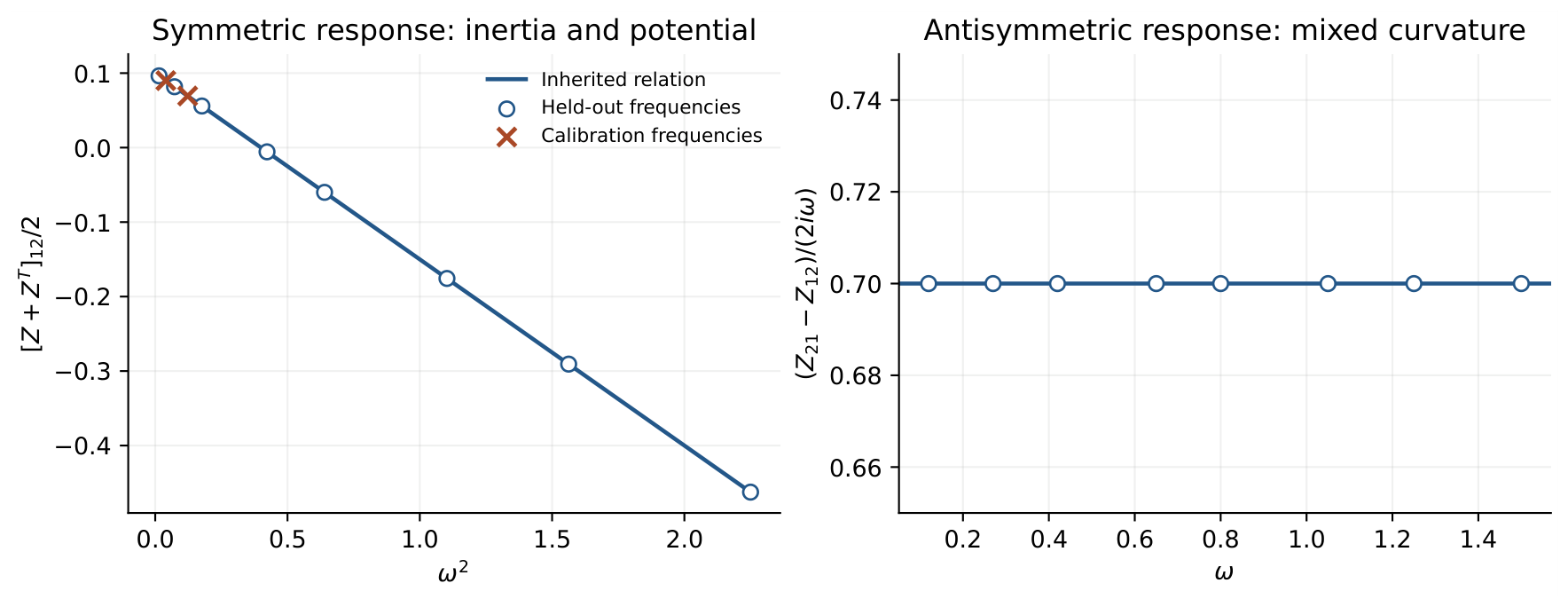
Declared full-rank input and readout maps are also used to test Eq. (A9). The program reconstructs the coefficients using only and then compares the complex responses at eight frequencies excluded from calibration. Figure A1 displays the structure of the reconstruction. These parameters and port matrices serve algebraic verification; they represent neither a realized apparatus nor experimental data. Errors are stored in results/verification.json, with the frequency-by-frequency results in a CSV file.
This appendix derives the forced response and identification conditions for a general local path, while Section 3 establishes a particular field realization. In particular, the path coordinate and the directional coordinate of the field channel have different definitions. The latter enters the gauge representation and can be related to an actual response only through an invariant formed with the parent connection and subject to the constraints. Correspondence between the two variational problems must be established through compatibility with both the constraints and the evolution.
Figure A1.
Response identification with synthetic parameters. Left: the off-diagonal element of the symmetric inverse response is linear in . Crosses mark the two calibration frequencies, and open circles mark the remaining frequencies. Right: the calibrated antisymmetric part recovers the same contracted mixed curvature. Solid lines are generated from the declared parameters. The figure checks the formulas and their implementation and supplies no experimental evidence.
Figure A1.
Response identification with synthetic parameters. Left: the off-diagonal element of the symmetric inverse response is linear in . Crosses mark the two calibration frequencies, and open circles mark the remaining frequencies. Right: the calibrated antisymmetric part recovers the same contracted mixed curvature. Solid lines are generated from the declared parameters. The figure checks the formulas and their implementation and supplies no experimental evidence.
Appendix B Initial-State Reconstruction, Omitted Modes, and Constraint Checks
Appendix B.1. Reconstructing the Initial State from a Matter Time Series
Once the coefficients have been calibrated, the matter equation and its first derivative formally yield
Higher derivatives amplify noise in measured data. An integral reconstruction over a finite record is therefore preferable. With the observability Gramian
and after subtracting the forced response due to the known input, the initial state is
An error estimate requires a specified state scaling and noise model. For a dimensionless state, additive record noise , and exactly known input and model coefficients, the reconstruction operator gives
The smallest eigenvalue controls the absolute error amplification in the least visible direction, whereas the condition number measures the relative ill-conditioning among directions. Both depend on the chosen state scaling. Correlated measurement noise requires a covariance-weighted information matrix.
Initial-state reconstruction and parameter identification are distinct questions. For the four-state model considered here, let denote the Laplace variable, to distinguish it from the primitive observation state s. The transfer function is
If u and x are independently calibrated, the model structure is known, and , the numerator and denominator have no common zero. The exact transfer function then uniquely determines the four combinations m, , , and : the numerator zeros determine a, the high-frequency coefficient determines m, and the constant and quadratic coefficients of the denominator determine and b. This conclusion includes ; the accuracy achievable in an experiment still depends on the available bandwidth and noise.
The remaining freedom in corresponds to the rescaling ,
A negative also reverses the orientation of f. Within this fixed model class, the ambiguity is a coordinate rescaling. Once a calibrated representative has been chosen, a complete time record reconstructs its four-dimensional initial state; the record does not independently fix an absolute observation scale.
Appendix B.2. Source-Profile Mismatch and Feedback from Omitted Modes
An actual current profile may contain additional transverse spatial modes. For an orthonormal spectral family , write , with and . The full quadratic equations give
For zero initial data in the omitted sector, each omitted mode is
Even when the initial field occupies a single mode, the source may subsequently excite others. An exact single-mode reduction therefore also requires the source to have no projection onto the orthogonal modes. If such projections are present, the matter equation receives feedback , and the omitted modes modify the harmonic impedance by
Near an omitted-mode resonance, the small denominator may magnify this correction, so that even a small overlap calls for a renewed error estimate. For a specified actual trajectory x, one also obtains
This bound estimates the excitation energy in the omitted field modes. Because those modes also act back on matter, their feedback must be included when comparing matter trajectories in the full and truncated models. A quantitative assessment of the single-mode approximation thus requires both the retained-mode overlap and the overlaps with the remaining modes.
Appendix B.3. Numerical Checks of the Field Reduction, Preparation, and Release
The numerical checks use the following dimensionless synthetic coefficients:
The spatial domain is the periodic interval , with normalized profile . Its vector direction is chosen either perpendicular or parallel to the wave vector. The two branches follow directly from the original coefficients:
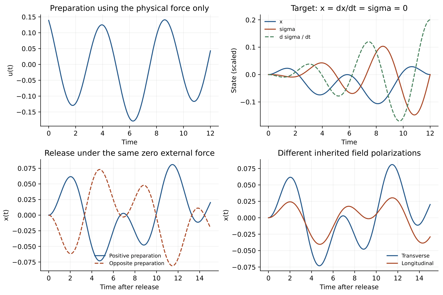
Starting from the zero state, the preparation lasts and targets . The control is determined by Eq. (31), with no external force added to the observation equation. The program independently integrates preparation, input work, and release, and substitutes the state into the spatial field equations and the Gauss constraint.
Table A1.
Numerical checks for the synthetic constrained reduction. All quantities use the stated dimensionless normalization. The reported errors are numerical errors, not experimental accuracies.
Table A1.
Numerical checks for the synthetic constrained reduction. All quantities use the stated dimensionless normalization. The reported errors are numerical errors, not experimental accuracies.
| Quantity | Transverse | Longitudinal |
|---|---|---|
| Maximum absolute terminal error | ||
| Maximum Gauss-constraint residual | 0 | |
| Maximum spatial field-equation residual | ||
| Maximum matter-equation residual | ||
| Physical input work | ||
| Squared-input integral | ||
| [l]Maximum reconstruction error | ||
| from an analytic matter record | ||
| Initial release acceleration |
Figure A2.
Preparation and release with one physical input. Upper left: the preparation force in the transverse branch. Upper right: the matter position returns to zero while the observation channel retains a nonzero velocity. Lower left: matter responses from opposite initial states under the same zero external force; the negative-preparation curve follows from linear symmetry. Lower right: transverse and longitudinal branches derived from the same parent coefficients. These are calculations within the stated model, not measurements from an apparatus.
Figure A2.
Preparation and release with one physical input. Upper left: the preparation force in the transverse branch. Upper right: the matter position returns to zero while the observation channel retains a nonzero velocity. Lower left: matter responses from opposite initial states under the same zero external force; the negative-preparation curve follows from linear symmetry. Lower right: transverse and longitudinal branches derived from the same parent coefficients. These are calculations within the stated model, not measurements from an apparatus.
The energy check uses the full constrained Hamiltonian, including the dynamical matter source. Since , the matter Legendre transform cancels the field term . Applying the Gauss constraint then gives
The difference between this expression and the reduced energy is below in both branches. During preparation, the maximum discrepancy between input work and energy change is below . The initial-state reconstruction uses an analytically generated matter time series, so its reported error checks only the integral reconstruction formula. The field, preparation, and release calculations are checked by independent integration of the differential equations. Sensor noise, sampling, and calibration errors are not included; readout accuracy must be assessed separately once those errors are incorporated.
Appendix C Dirac Matter Currents and a Cold-Flow Realization
Appendix C.1. From the Original Matter Current to Explicit Matter Modes
The finite-time preparation proof requires a nonzero current overlap, which must ultimately be supplied by a matter state. The fermionic sector of the unified-action study provides a calculable candidate. Counterflowing states can be constructed in its existing representation and generator direction, and their current, inertia, and field feedback determine the reduced coefficients. This construction also identifies the force and readout that an implementation would require. The derivation and its scale conditions are given below.
Appendix C.8.1. Operator Origin and Normalization of the Current
We use the source convention . The unified-action study already writes the bridge interaction as
and specifies together with the action of on the rank-two antisymmetric representation. It also retains a vectorlike Dirac field in the fundamental representation:
The modes used below are drawn from this existing vectorlike Dirac matter sector [6], with its representation and couplings unchanged.
To match the anti-Hermitian generator of the original channel, define , so that . Substitution into the Dirac kinetic term gives
The coupling sign follows the generator orientation. With the positive-coupling convention of Eq. (A26), the field and source must instead be related by . Their normalization must preserve this product. Inserting the same coupling both into the field redefinition and into the current would change the original action.
Along the selected normalized bridge direction, . The canonically normalized field is , with coupling . The value of Z is that of the original common background, including the vacuum contribution prescribed in the source study.
Appendix C.8.2. States That Can Carry a Bridge Current
On the two original basis vectors connected by the bridge, choose
These matrices are embedded in the original fundamental representation, leaving the remaining directions unchanged. Thus . A matter wavefunction confined entirely to one block carries exactly zero current in this channel. For a mixed state, the more general criterion applies separately to each spacetime component: if the internal bilinear matrix entering is block diagonal with respect to the two blocks, its trace pairing with vanishes. Equation (A28) therefore depends on the cross-block part of the internal bilinear and cannot be inferred from ordinary charge numbers alone.
The chosen must be specified together with the actual response direction and the reference used to prepare the internal state. Under a common change of frame, both and the matter bilinear transform by conjugation, leaving their trace pairing invariant. A bare matrix component, with no retained physical reference, cannot itself be identified as an observable. Preparation, preservation, and readout of cross-block coherence must all use the common reference. The calculation here specifies a candidate source; it does not supply an experimental construction of that reference.
Number density does not determine the entire current. A block-diagonal internal number density makes the corresponding time component vanish, but correlations between internal state and velocity can leave cross-block components in the spatial current. Counterflow provides an example.
Appendix C.8.3. Counterflowing States of the Original Dirac Matter
Take the eigenstates of ,
The singlet mass in Eq. (A27) is proportional to the identity in the fundamental representation and therefore does not split these states at this level. Assign each state number density , and give each of the remaining three internal states the same number density while keeping them at rest in the background. The total internal number-density matrix is . Consider the transverse displacements
All quantities are independent of y, so the shear neither changes the density nor produces a charge-density perturbation. The spatial current matrix of the two streams is
Taking its trace pairing with the original generator family yields
With the common trace-orthogonal normalization, the linear currents in the remaining directions vanish. This trace pairing also determines the projections of the matter source onto the other generators. It holds in the stated low-velocity convective approximation without spin polarization; it does not eliminate spin or transition matrix elements from the Dirac theory.
More precisely, we use a long-wavelength, low-velocity dynamical approximation for dilute positive-energy wave packets, neglecting pressure, collisions, spin magnetization, and quantum-gradient stresses. This requires and relevant frequencies and wavenumbers satisfying , together with control of field strength, velocity spread, and wave-packet dispersion. Finite-density fermionic matter cannot simply be replaced by a classical flow at strictly zero temperature and zero momentum spread; the validity of these approximations must be tested in a further quantum-matter calculation. At this order, a single wave packet has worldline action . Substituting velocities and charges , and subtracting the rest energy already included in the background, gives
Here h is the physical force density acting on the relative motion; the conditions on its source are discussed below in the selective-force analysis. Uniform shear has no confining or elastic energy in this approximation. Its matter restoring force therefore vanishes, giving the case admitted by the preparation theorem.
Equation (A34) realizes the original matter content under the stated approximation; it is not an exact finite-mode truncation of the full Dirac equation. The three stationary states still contribute background mass and scalar sources, and the total static mass density is . These sources must be included in a solution for the common background or treated within a verifiable local approximation of weak backreaction. Counterflow cancels the total mass current to first order. Kinetic energy is already retained in the quadratic action; its backreaction on the background and longitudinal motion begins at second order in amplitude, as does the longitudinal magnetic force. If the background masses split, or if other interactions fail to conserve the charge, internal-state evolution must be retained and no longer defines a closed current.
Appendix C.8.4. A Common Density Fixes Both Inertia and Coupling
Variation of Eq. (A34) gives
Since , , and , the Gauss equation gives . With periodic or no-flux boundaries, energy and input work satisfy
The mixed velocity term cancels in the full Legendre transform. The first equation of motion makes the current evolve jointly with the field; prescribing the current as an external source would remove this feedback.
On a uniform background , choose a common real mode satisfying , and set . With and , the reduced coefficients are
The profile in the constrained reduction is thus : its shape and amplitude are fixed by the same matter mode. Mode normalization changes the generalized coordinates and coefficients, but leaves
unchanged. Because the same density enters inertia and coupling, these are no longer independent fit parameters. The final term comes from feedback by the same matter current and shifts the nonzero oscillation frequency of the coupled system. It does not redefine the bridge mass in vacuum.
The shift can also be checked directly in the spatial equations. After release, , and the first equation implies
The function is fixed by the terminal preparation state and must be retained. At uniform density, the homogeneous frequency is precisely Eq. (A38). A nonuniform density changes the spatial response operator and requires its modes to be recalculated.
Appendix C.2. Selective Forcing and Current Readout
Appendix C.9.1. The Drive Must Act on Relative Motion
Restore the common displacement Y of the two streams by writing . Let the external transverse forces on each particle be and , respectively. The linear term in the driving action is
The two streams have equal masses. An ordinary force of equal magnitude and direction, , drives only Y and supplies no input to the relative equation. Single-input preparation requires a specified force difference with spatial overlap
If an existing control coupling distinguishes the two internal states, one amplitude parameter can supply this force difference. The controllability proof assumes such a selective coupling; its form and strength must still be derived from the original matter action.
For a purely common drive and zero initial field and relative flow, Eq. (A35) has the unique linear evolution . This arrangement does not excite the channel under study. The zero response rules out common driving alone as a preparation method for this channel; controllability remains valid when a relative input is available.
Appendix C.9.2. Current Records Retain Field Initial-State Information Without Position Markers
A constant displacement of a uniform shear flow changes neither its Eulerian density nor its current. Without trackable labels or boundary markers, the full position is therefore unavailable as a record in the present flow model. The matter response contains the relative velocity , or the corresponding bridge current . Because the ordinary total mass current cancels between the counterflowing streams, the record must resolve their internal states or the associated weighted current. A specific detection coupling is still required.
Assuming that this record is available and the parameters have been calibrated, take , with . The retained dynamics are
Direct calculation gives
Thus, for and , all three quantities can be prepared by a relative physical force and recovered from a complete relative-velocity record. The constant displacement of an unmarked flow is absent from these three variables accessible to readout, whereas the field amplitude and field velocity are both retained. Formally,
For noisy data, reconstruction should again use time integrals rather than direct higher differentiation. If reliable position markers are also available, the four-dimensional position-readout model and its terminal-position condition remain applicable. The current readout considered here instead corresponds to a three-dimensional state.
Appendix C.3. Joint Closure of Matter and Field Modes
The spatial spectrum of a matter source may excite omitted field modes, and the field may in turn drive additional matter modes. A single-mode reduction must therefore be closed in both directions.
For general matter eigenmodes and field eigenmodes , define the current overlaps . In a basis in which the matter inertia and potential, and the field inertia and potential, respect the selected eigenmode blocks, a mode pair can form an invariant subsystem only if
and the input, initial state, and other retained couplings have no orthogonal components. The first condition closes the field equation, and the second closes the matter equation. If the mass matrix is not diagonal, the corresponding generalized eigenvalue decomposition must be performed first, or the invariant subspace of the full dynamical matrix must be checked directly. Inspection of one row and one column of G alone is then insufficient.
In this cold-flow model, even density, initial data, and driving force preserve the even-parity subspace. Within that subspace, use the periodic cosine basis , . Expanding and B over gives
Here F is the generalized force already projected onto relative motion. For ,
and all other off-diagonal elements vanish. The condition ensures a positive density and a positive-definite mass matrix. At uniform density, each spatial mode evolves independently. At nonuniform density, motion in couples to and further modes. Because the density also changes the mass matrix, modifying the coupling while leaving the inertia fixed would be inconsistent.
For zero initial data, Eq. (A46) has a direct first integral. With ,
The preparation impulse remains as an inhomogeneous source on the right, while the density correction to the field spectrum enters the operator on the left. The numerical calculation nevertheless integrates the full matter and field equations, using this identity as an independent check.
The multimode energy is
For nonuniform density, the matter kinetic energy contains cross terms. The omitted energy reported below therefore includes only orthogonal field modes and does not assign separate modal energies to those matter terms. Calculations at finite N must also be compared with larger truncations. This is a spectral convergence check, not by itself a proof for the infinite-dimensional equations.
Appendix C.4. Cold-Flow Numerical Results and Scale Conditions
The numerical calculation uses synthetic parameters in natural units,
These parameters test the implementation of the cold-flow equations. The high-energy benchmark of the unified-action study is used separately in the relativistic calculation. At uniform density, choose and recompute the force for the branch with the Gramian formula. Preparation lasts and targets . The condition is retained as a stronger mathematical endpoint requirement; without position markers, its absolute constant offset is not treated as a physical quantity accessible to readout. The system then evolves freely for 15 time units. All three density profiles receive the same relative force density , with no adjustment of the generalized input based on the output. Since , the corresponding force difference per particle is
Fixing the force density therefore does not fix the control force on each particle. If an experiment instead holds a selective external field fixed, the drive vector must be reprojected using and varied with the density in the comparison.
For these parameters, the energy in additional field modes generated by nonuniformity is small, although other matter modes already move during preparation. The field-energy fraction alone is therefore not a sufficient measure of the accuracy of the full reduction. Table A2 reports field energy and matter velocity separately. Holding the input fixed also allows the deviations to be traced to the changed density and inertia.
Table A2.
Synthetic cold-flow examples with . The retained-state error is the maximum absolute difference in the stated dimensionless variables; field-energy entries are fractions. The final column gives the maximum norm of the matter-velocity coefficients with over the full calculation interval.
Table A2.
Synthetic cold-flow examples with . The retained-state error is the maximum absolute difference in the stated dimensionless variables; field-energy entries are fractions. The final column gives the maximum norm of the matter-velocity coefficients with over the full calculation interval.
| Terminal retained-state error |
Omitted field- energy fraction |
Omitted velocity- mode norm |
|
|---|---|---|---|
| 0 | 0 | 0 | |
The program independently integrates input work and total impulse for the same process. The maximum discrepancy between energy change and input work is below , and the residual of Eq. (A48) is below . The energy at the end of preparation is approximately . The squared-input integral is and is not a physical energy. The total impulse at the preparation endpoint is close to zero, as required by the first integral.
Increasing the highest mode from to changes the retained state by less than . For , the maximum sampled residual of the full equations, reconstructed directly in space, decreases from to . Although the projected residual on the retained modes is already at roundoff level, a residual outside the truncation remains. The two must be distinguished: the former does not establish exact satisfaction of the full field equations. This convergence check covers only the stated interval and parameters.
The cold-flow approximation also requires sufficient separation between the frequencies, wavenumbers, and field amplitude and the matter mass. At , the highest retained coupled frequency divided by the matter mass is approximately , and the largest wavenumber divided by the mass is . The maximum spatial relative velocities in the three examples are , , and , respectively, with . These ratios check the retained spectrum and state amplitudes. The actual bandwidth and switching transients of the ideal preparation force still require control. The ratios are consistent with the chosen low-velocity, small-field approximation, but do not replace calculations of internal-state lifetimes, fermionic momentum spread, spin effects, or quantum-gradient corrections.
Figure A3.
Multimode calculation of cold-flow matter and the field. Upper left: the overlap matrix fixed by the density. Upper right: computed displacement after release, which corresponds directly to a displacement record only when position markers are available. Lower left: the energy in other field modes as a percentage of total energy; the dashed line marks release. Lower right: terminal deviations under the same input. All results are synthetic.
Figure A3.
Multimode calculation of cold-flow matter and the field. Upper left: the overlap matrix fixed by the density. Upper right: computed displacement after release, which corresponds directly to a displacement record only when position markers are available. Lower left: the energy in other field modes as a percentage of total energy; the dashed line marks release. Lower right: terminal deviations under the same input. All results are synthetic.
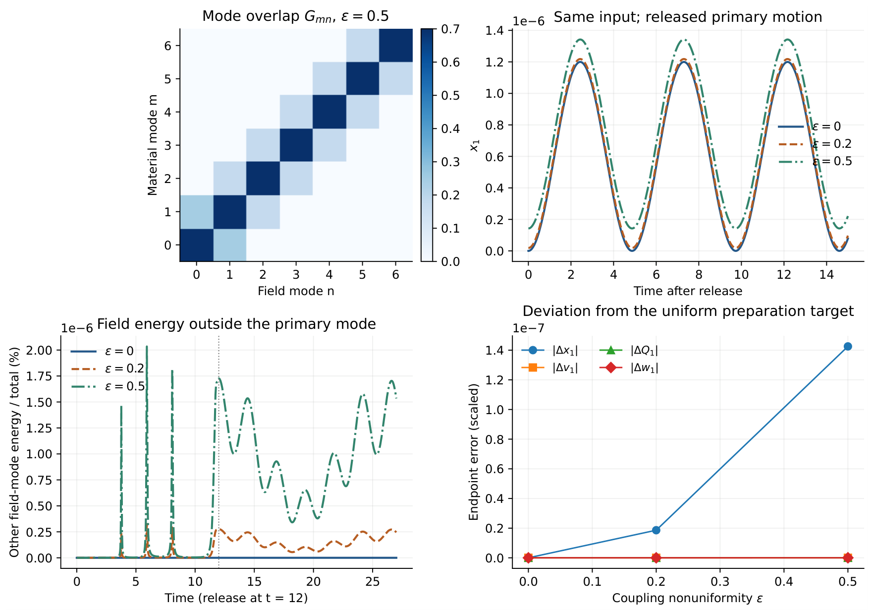
A separate source-matrix program runs over all 24 normalized generators of the fundamental representation. It verifies vanishing static traceless charges, a linear spatial current confined to the chosen bridge direction, and invariance of the trace pairing under a common change of frame. Residuals of the source and normalization identities are below . The three-state controllability and observability determinants also agree with Eq. (A43). The programs are verifymattersources.py and verifymattermodes.py; their parameters, energy definitions, and calculation domains are recorded in the source code and JSON results.
Appendix D Relativistic Vacuum Response and the Scope of the Quantum Approximation
Appendix D.1. Bridge-Field Dynamics Beyond the Cold-Flow Approximation
Appendix D.12.1. Matter Content, Masses, and Perturbative Order
Let denote the canonically normalized bridge field, with its source defined as in the unified-action study:
Here T is a real bridge generator in the original fundamental representation, with . We retain the original benchmark,
In the leading-order width below, takes the original tree-level matched value. Loop corrections affect both the real part of the pole and its residue. A corrected mass therefore requires finite mass and kinetic matching within a single renormalization scheme, as prescribed in the unified-action study. The bare mass and the corrected pole mass have distinct roles in this calculation; a given numerical value cannot serve as both.
We calculate the one-loop contribution of mass-degenerate Dirac matter to the transverse channel in an internally unbiased vacuum. The vacuum kernel provides an explicit benchmark for relativistic response. The finite-density preparation state of the cold-flow model also carries a particle distribution and initial correlations, and its medium corrections depend on these additional inputs. Loops of other fields already present in the theory may contribute to propagation and decay. The numbers in this section thus refer only to this Dirac matter channel; the total width requires all open channels.
Appendix D.2. Relativistic Current Response and the Absorption Threshold
We use signature , Fourier convention , and units . The Dirac matrices obey , consistently with the positive-energy Dirac equation in Eq. (A52). Write ; the distinct typeface separates this invariant from the primitive observation state s used above. For we take the retarded boundary value, with negative frequencies fixed by the conjugation relation for a real response. The causal response of a current to a weak source is the setting of linear-response theory [18]. Here, integrating out the Dirac field and taking the second variation of the one-loop effective action with respect to the test source gives the vacuum current two-point kernel. The internal trace in the Dirac loop yields , while the spin trace and Feynman-parameter integral give the transverse scalar function
The subscript 0 denotes subtraction at zero momentum, . This expression retains arbitrary and makes no nonrelativistic expansion.
To see its structure, combine the two fermion denominators and shift the loop momentum. The remaining parameter denominator is . With a regulator that preserves the vector-current Ward identity [19], the longitudinal terms cancel and the tensor structure is proportional to , so that . Subtracting the value at removes the ultraviolet constant and leaves the logarithm in Eq. (A54). This is the standard loop calculation for the original Dirac term; Ref. [20] provides the Feynman parameterization and transverse decomposition, while the group factor and numerical parameters follow from the original common action.
For a spatially transverse polarization, write the free inverse kernel as . Including this matter loop gives
where is the real local term associated with the chosen renormalization conditions. The real part of depends on the subtraction convention; real local terms do not remove the absorptive contribution of an open channel at this order. The line shape near a specified pole mass can be obtained by matching the real part of the pole and its residue within the same scheme. The numerical real part after zero-momentum subtraction alone does not determine the corrected physical mass.
Appendix D.13.1. The Threshold from the Same Integral
The logarithm develops an imaginary part only where . Such an interval exists for , with endpoints
Since , Eq. (A54) gives
Absorption at positive frequency is nonnegative. It gives a positive imaginary part on the physical real axis, placing the weak-coupling pole in the lower half of the frequency plane, as required for decay in time. The two-body phase-space calculation below independently checks this sign.
For , expansion of the logarithm yields
At large positive ,
The original benchmark has and lies well inside the relativistic regime. Its response must be calculated from the full kernel or the high-energy expansion; the cold-flow frequency formula no longer applies at this scale.
Appendix D.3. The Partial width at the Fixed Benchmark
For one real bridge vector field, summing over final spins and internal states and averaging over the three initial polarizations gives
For the open channel , the two-body phase space then gives
This equals . The factor already includes all internal states in the fundamental representation, so no additional factor of 5 is required. In the eigenbasis of T, the nonzero charges are and , whose squares sum to ; the other three states do not couple along this generator.
The threshold ratio and partial width at the original benchmark are
This leading-order partial width shows that real fermion-pair final states are already open at the original benchmark. Other open channels in the common theory will increase the total width and shorten the lifetime. Their contributions must be calculated from their respective couplings and phase spaces and are not included in Eq. (A62), which is a theoretical value for the specified channel.
In the rest frame , assuming narrow-pole dominance and retaining only this partial width, the amplitude envelope is , while the energy or survival-probability envelope is . Taking as the free oscillation period, the amplitude falls to in approximately periods and the survival probability falls to in approximately periods. The squared relation makes the latter decay time exactly half the former. The full response also contains the threshold branch cut, whose relative contribution varies with the time scale. A single exponential therefore applies only during the evolution dominated by the narrow pole.
Appendix D.4. Excitation and Readout of the Bridge Channel Through Matter Control
Appendix D.15.1. Current-Matrix Overlaps and Linear Response
Suppose matter control acts through , with , and the readout corresponds to . Here is the test source used to calculate the response; its interpretation as an experimental input also depends on its coupling to an actual matter control.
Define the retarded response to by , or , with spatial arguments and the appropriate indices understood. In a mass-degenerate, internally unbiased vacuum, the internal propagator in the one-loop calculation is proportional to the identity. Hence
with local contact terms matched in the same subtraction convention. For spatially transverse components, .
Linear coupling of the preparation source to the selected channel therefore requires , while retaining that channel in the readout requires . If R is proportional to the identity or is block diagonal with respect to the original two response blocks, and T connects only the two blocks, then . The relativistic vacuum response thus reproduces the selection result for common driving in the cold-flow model. This rule follows from the internal trace structure on the present background. A change in the matter state, coupling, or expansion order can change the propagator and response tensor, requiring the selection rule to be reassessed.
The matrices transform together with the common response reference, leaving and invariant. The selection rule is therefore independent of the representation basis. The formal choices or yield nonzero overlaps; realizing these algebraic choices as preparation and readout still requires the corresponding control couplings and recording procedures.
Appendix D.15.2. A Common Propagation Kernel for Preparation and Readout
For spatially transverse components, variation of the action gives . Substitution of the current response above yields the consistent input–output relations
The same renormalization and contact-term conventions are used throughout. The first term is the direct matter response to the control, and the second contains bridge propagation. Both enter the experimental record. Identifying bridge propagation therefore requires either independent calibration of the direct response or its retention in the full model.
In the time domain, products become retarded convolutions. Even if is switched off at the end of preparation, the direct response can persist, and the bridge-field evolution likewise retains the influence of earlier excitation. Equation (A64) specifies the causal relation between a given source and readout. The full experimental waveform also depends on the spacetime profile of the source and the matter state actually prepared.
Appendix D.15.3. The Quantum Approximation Underlying the Response Formula
Equation (A64) follows from the one-loop effective action of the Dirac field by retaining terms quadratic in the test source and bridge field and then eliminating the bridge field. Thus is the one-loop irreducible current kernel, while is resummed within this quadratic effective theory. The equality holds in this Gaussian reduction.
This approximation has direct consequences for the experimental criteria. Away from resonance, the bridge-exchange term contains two current loops joined by field propagation. Irreducible current corrections with internal interaction lines may arise at the same order in the coupling. Subtracting only the free Dirac-loop term does not remove these corrections from an experimental residual. Propagation enhancement near a pole can make the pole term dominant, but its accuracy still requires consistent power counting and matching [21]. These higher-order terms are not calculated here. The vanishing minors and fixed amplitude ratios below are therefore exact relations of the stated quadratic effective model and require a theoretical uncertainty when used as experimental predictions.
Denoting the reduced response by , the physical prediction should be written as
The remainder includes omitted irreducible corrections, other channels already present in the theory, and medium contributions from the actual matter state. Each must be calculated or bounded within the same matching scheme; machine roundoff cannot represent this theoretical uncertainty. If the direct term has been extended to the full irreducible source–source block and the effective mediator is one-dimensional, the Schur complement retains an outer-product structure. Its vertices and background, however, no longer automatically equal the one-loop expressions used here.
The definition of the source also enters the matching. The field–field, field–source, and source–source quadratic terms in the fermion effective action arise from the same expansion, and their finite contact terms must be treated consistently. The propagation-kernel inversion below acquires a definite experimental meaning only when these local terms and the normalization of the actual sources and readouts have been fixed together.
Appendix D.5. The Continuous Spectrum and Finite-Dimensional Preparation
The four-state theorem in Sec. Section 4 applies to a closed, nondissipative quadratic system with constant coefficients. The full relativistic kernel considered here has a branch point and continuous spectrum at . A finite-dimensional linear system with constant coefficients has a rational transfer function; a response containing this logarithmic branch cut cannot be represented exactly over all frequencies by those four states. At the original high-energy benchmark, applying Gramian control to this channel therefore requires a frequency-band reduction and an error analysis.
Preparation and readout consequently require a reduction with a specified bandwidth and accuracy. For a chosen initial state and operating band, one must determine how accurately a few poles approximate the full kernel and how the control waveform must be adjusted. Even if only a weakly damped pole is retained, the deviation accumulated by a nondissipative waveform can be estimated. In dimensionless time , at the partial width above alone reduces the amplitude envelope by about and the energy or probability envelope by about . The value 12 illustrates the error on this time scale; the preparation time in the finite-dimensional synthetic example must still be converted using its own units and parameters.
The finite-density preparation state of the cold-flow model introduces a further dependence: the actual particle distribution and any necessary initial correlations change the medium response and must be calculated from the same action. The corresponding selective source and internally resolved readout also require explicit physical realizations. Equations (A63) and (A64) express these requirements as verifiable matrix overlaps and response relations, with the vacuum kernel providing the benchmark for the analysis.
Appendix D.6. Independent Checks of the Response Kernel and Partial Width
The numerical checks use independent integrations and matrix calculations. The real part of Eq. (A54) is integrated piecewise across the logarithmic zeros, while the imaginary part is integrated separately over the absorption interval. The width is also calculated directly from the spin trace of four-dimensional Dirac matrices and the two-body phase space. The three calculations share the same generator normalization and cover both sides of the threshold, the low-energy expansion, and the original high-energy benchmark. Table A3 and Figure A4 give the results.
Table A3.
Independent numerical checks of the relativistic response. Errors are absolute differences at the sampled points; the relevant functions and width ratios are dimensionless.
Table A3.
Independent numerical checks of the relativistic response. Errors are absolute differences at the sampled points; the relevant functions and width ratios are dimensionless.
| Check | Result |
|---|---|
| Maximum difference between absorption-interval integration and the analytic imaginary part | |
| Maximum difference between the Dirac trace with phase space and | |
| Difference between the threshold real part and | |
| at the original benchmark | |
| at the original benchmark | |
| Trace pairing of identity or block-diagonal sources with T | 0 |
| Trace pairing for the matched test source |
The numerical real part belongs to the subtraction convention . It checks the integral and its asymptotic forms but does not directly determine the corrected physical mass. The two independent width calculations agree within floating-point precision, verifying the absorption sign, phase space, and internal-state counting. Such numerical agreement does not replace an error estimate for higher-order terms or the actual matter state.
Figure A4.
Dirac-channel response at the fixed original parameters. Upper left: real and imaginary parts after zero-momentum subtraction. Upper right: the two-body threshold, with points from independent integration over the absorption interval. Lower left: the near-pole line shape after matching the real part of the pole and retaining only the absorptive term; full dispersion and other channels are omitted. Lower right: narrow-pole amplitude and energy or probability envelopes, retaining only this partial width, with time . The lower panels illustrate the stated approximations and do not give the exact evolution of the full branch-cut response.
Figure A4.
Dirac-channel response at the fixed original parameters. Upper left: real and imaginary parts after zero-momentum subtraction. Upper right: the two-body threshold, with points from independent integration over the absorption interval. Lower left: the near-pole line shape after matching the real part of the pole and retaining only the absorptive term; full dispersion and other channels are omitted. Lower right: narrow-pole amplitude and energy or probability envelopes, retaining only this partial width, with time . The lower panels illustrate the stated approximations and do not give the exact evolution of the full branch-cut response.
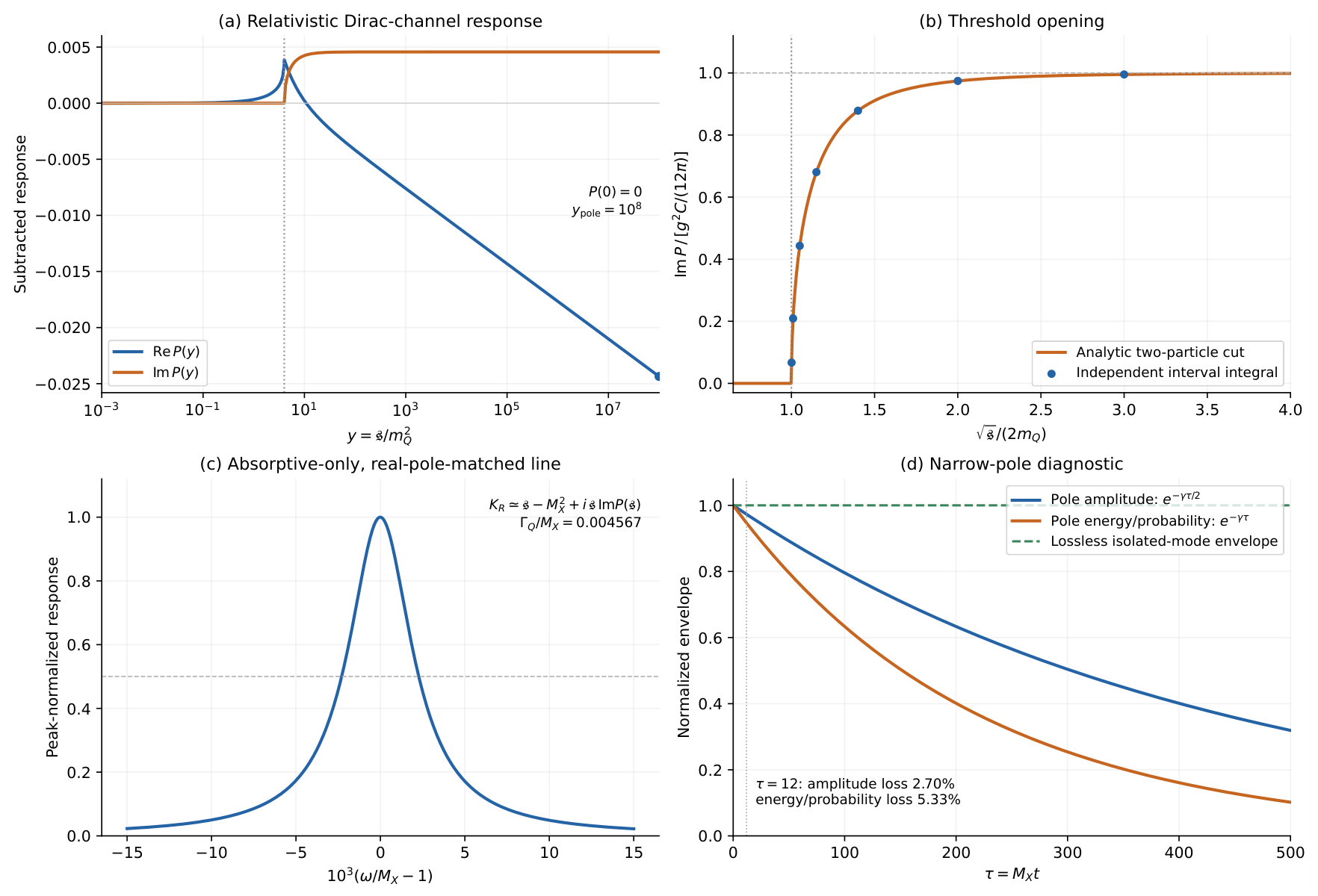
Appendix E Multiple-Source Response and Indirect Tests of Common Parameters
Appendix E.1. Common Response Relations Between Sources and Readouts
Appendix E.18.1. One Channel and a Common Frequency Function
Fix the spatially transverse polarization, wavenumber, and common matter reference. Let the available sources be and the readouts , and define
In this section, L denotes only the scalar part of the current kernel. The source and readout matrices are Hermitian. The following formulas come from the one-loop quadratic effective action in Appendix D and assume that propagation along the selected T direction has been isolated. We have not established whether an actual control can achieve this isolation. After independent calibration of input amplitude and phase, spatial profile, and readout transfer, Eq. (A64) becomes
The first term is the direct matter response. Subtracting it with the same subtraction and contact-term conventions defines
Changes of source and readout enter through the overlap coefficients, while all frequency dependence resides in a single function. The records therefore obey relations that can be checked against one another, beyond fitting each curve separately.
For any two sources and two readouts,
More generally, the residual matrix has rank at most one at every frequency. Whenever the reference channel is nonzero,
The first ratio is independent of frequency. Since the traces are real, the phase difference between the corresponding nonzero residuals is 0 or . The second ratio is independent of the chosen source and readout. For weak responses, the equivalent cross-multiplied relations are preferable to division by records close to zero.
Equation (A69) gives a direct held-out test: three complex responses predict the fourth,
The fourth record is reserved for independent validation and does not enter the adjustment of the first three coefficients. Equation (A70) and the explicit form of further constrain amplitude ratios and frequency dependence, supplying information beyond the rank-one structure itself.
Rank one at each frequency follows from an isolated one-dimensional mediator and can persist for more general dispersive vertices. Frequency-independent amplitude ratios and the phase relation additionally require mass degeneracy, an internally unbiased vacuum, and fixed source and readout matrices. Finite density, mass splitting, or dispersion in the input requires a corresponding modification of the kernel. If other bridge directions of the original theory contribute, the matrix formulation below applies.
Appendix E.18.2. Several Bridge Directions Sharing a Pole
The bridge subspace in the unified-action study contains twelve real directions whose tree-level masses are set by the same background [6]. When a source or readout couples to several directions at once, the single-axis expression must be extended. Let range over the retained bridge directions and define
With the same degenerate Dirac kernel and common coupling convention, eliminating these bridge fields gives
Here is the inverse propagation kernel in the space of bridge directions. Away from poles, if r directions are retained,
The rank is determined jointly by propagation and by the directions that can actually be excited and read out. Even an observed rank of one may mean that the ports project only one combination of a multichannel system.
If , all these directions have exactly the same frequency function, and
A common pole and fixed complex amplitude ratios may survive without rank one. For an explicit example, using matrix indices beginning at zero, take
Both are directions in the original bridge subspace. Setting gives
The rank is two whenever . This result is compatible with the original action, and a frequency scan cannot separate two exactly degenerate directions. Before applying Eq. (A69), one must therefore establish the effective single-axis condition from the source, readout, and propagation matrices together. If several directions are retained, the appropriate test is Eq. (A73).
Figure A5.
Responses of a single bridge axis and two degenerate bridge axes, normalized by , with as sources and readouts. The left panel retains only the contribution; the right retains both directions. They can share the same pole while their response matrices have ranks one and two, respectively. The entries follow from matrix-trace identities.
Figure A5.
Responses of a single bridge axis and two degenerate bridge axes, normalized by , with as sources and readouts. The left panel retains only the contribution; the right retains both directions. They can share the same pole while their response matrices have ranks one and two, respectively. The entries follow from matrix-trace identities.
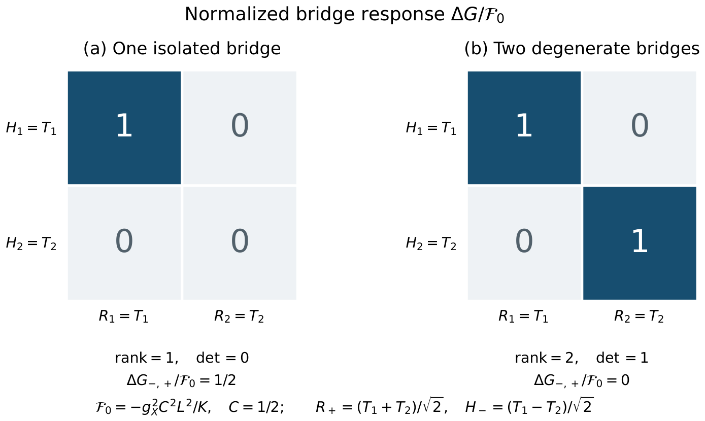
Appendix E.18.3. Orthogonal Controls and Direction Reversal
Choose a matrix U satisfying and . If the physical control can realize
then, with fixed readout , the bridge residual obeys
Thus provides a zero-residual control, and reverses the residual sign. The reversal concerns the actual control relative to the common matter reference. A simultaneous change of basis for all matrices leaves their trace pairings unchanged and produces no new signal.
One can also test a combination with a vanishing direct term. If available controls allow and , then
This expression removes the one-loop direct term of the present Dirac kernel and assumes that the single-axis contribution of T has been isolated. If is another bridge direction already present in the theory and is exactly degenerate with , the two bridge contributions are and , respectively, and cancel. A zero direct term therefore does not guarantee a nonzero remaining single-axis signal. An actual test must identify all original directions participating in propagation, together with the medium response and instrumental background.
Appendix E.2. Complex-Response Measurements and Independent Predictions
Appendix E.19.1. Calibration and Held-Out Records
An experimental design must begin with realizable control terms, readout operators, matter states, and spatial profiles. The smallest nontrivial matrix test requires two independent sources and two independent readouts. The data may be acquired sequentially, without introducing additional physical fields. Input and readout gain, phase, crosstalk, and the common reference should be calibrated before testing the response.
Within the weak-excitation regime, the complex response should be measured at several source strengths to check that the output scales linearly with the input. Frequency points should span the same accessible band, with a consistent source profile and matter preparation. Coherent measurements provide both amplitude and phase; intensity alone cannot fully test the complex cross-relations.
The direct matter term requires independent constraints, and its uncertainty must be propagated into the residual. Allowing the background to vary freely at each frequency would deprive the rank-one relation of its testing power. The finite real local matching coefficients allowed by the original action should be determined from calibration data selected in advance; the remaining frequency points then test whether those coefficients make consistent predictions. The kernels reconstructed from individual nonzero records,
should agree. This agreement concerns the propagation kernel and complex poles. Frequency dependence in the direct background and numerator can shift the maxima of the raw curves, so a common pole does not require their peaks to coincide.
Figure A6.
Control and readout relations required for a direct response test. The boxes specify couplings and analysis steps; hardware depends on how those couplings are realized. The dashed direct term enters the record together with bridge propagation, and its contribution and uncertainty must be retained in the analysis.
Figure A6.
Control and readout relations required for a direct response test. The boxes specify couplings and analysis steps; hardware depends on how those couplings are realized. The dashed direct term enters the record together with bridge propagation, and its contribution and uncertainty must be retained in the analysis.
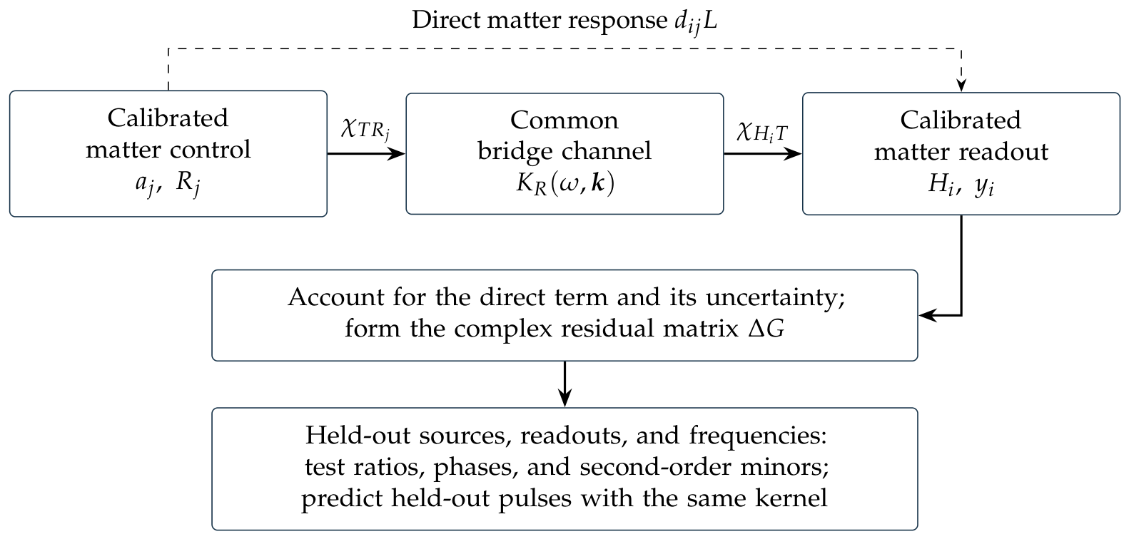
Arrange the real and imaginary parts of the held-out records in a vector , with prediction , and let be the full covariance of the prediction residual. A possible test statistic is
The covariance must include uncertainties and correlations in the held-out records, the responses used for prediction, the direct term, and the calibration parameters. Likelihood-based analyses likewise retain calibration parameters and systematic effects in the statistical model [22]. The noise distribution and fitting constraints determine the degrees of freedom and significance of the statistic. We can therefore specify the form of the test, but numerical thresholds require real noise data. Correlated errors can also make elementwise rescaling followed by singular-value analysis inadequate; assessment must use the full covariance.
The theoretical remainder should be treated separately from measurement error. Where a credible probability model exists, its correlations can be propagated into the prediction covariance. Where only bounds are available, it is more appropriately included as a bounded bias or nuisance parameter. Without an estimate of the remainder, Eq. (A82) assesses only the agreement between data and the stated approximation. A nonzero minor alone cannot then be interpreted as excluding the full action.
Appendix E.19.2. Thresholds, Widths, and Response After Release
The absorptive part extracted from the common kernel should turn on at . With , Eq. (A57) gives
This square-root law is the one-loop threshold behavior of a free Dirac pair. An experimental comparison must select a frequency band in which higher-order final-state interactions are controlled; their uncertainty extremely close to threshold is not estimated here. The square-root onset concerns the absorptive kernel extracted from the records. Raw signals between different sources and readouts also contain overlap coefficients, the direct term, and the propagation denominator. Their imaginary parts must be converted through these relations before comparison with Eq. (A83).
If a resonance experiment can resolve the final state, it should measure both the total width and the branching fraction , using
to test the relativistically calculated partial width. Other open channels of the original action also contribute to the total line width. The branching fraction supplies the information needed to isolate the target channel and compare it with .
After frequency-domain calibration, a finite-duration source waveform not used for calibration can be selected to predict all records,
This formula assumes a forced linear response about the same equilibrium initial state. An independently prepared nonequilibrium initial state requires an additional initial-state term. Switching the source off at the endpoint does not remove the direct matter convolution left by previous excitation. In the rest frame , if a segment of the release record is dominated by a narrow pole, the amplitude envelope should follow . Its decay constant is fixed by the same frequency-domain pole, with no additional free constant introduced in the time domain.
A further test of how the observation initial state affects matter evolution requires two constraint-satisfying joint initial states with identical retained physical initial data, subsequent external sources, and readout, but different prescribed observation initial data. The actual preparation must supply the corresponding map and record its effects on other matter and continuum states. This high-energy preparation map has not been determined by the vacuum response kernel, and finite-density preparations contain information absent from that kernel. The protocol above specifies how responses should be measured and compared; actual preparation of the observation initial state still requires a control realization derived within the same action.
Appendix E.3. Direct-Experiment Constraints at the Original High-Energy Benchmark
Converting the original benchmark into customary experimental units makes the required scales explicit. Using as in the unified-action study gives Table A4.
Table A4.
Scales for direct tests at the original parameters. The last two rows retain only the relativistically calculated Dirac partial width and use the narrow-pole approximation.
Table A4.
Scales for direct tests at the original parameters. The last two rows retain only the relativistically calculated Dirac partial width and use the narrow-pole approximation.
| Quantity | Original benchmark |
|---|---|
| Fermion-pair threshold | |
| Bridge resonance energy | |
| Rest-frame ordinary frequency | |
| Reduced length | |
| Probability-envelope time | |
| Amplitude-envelope time |
Compared with the proton collision energy already reached at the LHC [23], the two-body threshold is higher by about and the bridge resonance energy by about . On-shell resonance and threshold scans at the original parameters are therefore beyond the energy range of existing accelerators, with particle production as the primary obstacle. The extremely high frequency in the table does not imply that electronics must sample each cycle: if the particles can be produced, their properties can be inferred from mass spectra and final-state statistics.
A large mass does not eliminate the low-frequency response. Below the two-body threshold, absorption in this vacuum Dirac-pair channel vanishes, while the real part remains determined by Eq. (A54). The low-energy expansion in Eq. (A58) applies only for ; the full integral is needed near threshold. Finite-density matter may carry additional excitations and dissipation whose magnitudes depend on the actual distribution. We retain the original mass benchmark here. Experiments using lower-mass realizations would require a separate derivation relating their parameters to the original common background.
Appendix E.4. Low-Energy Indirect Tests of the Same Bridge Parameters
Appendix E.21.1. The Proton-Decay Prediction of the Unified-Action Study
Even when high-energy bridge particles cannot be produced on shell, their virtual exchange can affect low-energy processes. The separation of heavy-particle effects into renormalized couplings and suppressed low-energy operators has its standard field-theoretic basis in decoupling [24]. For the specified PODA realization, the unified-action study obtains, from the same mass and coupling [6],
These currents belong to the light chiral and representations already present in the unified action, with the sum extending over the original bridge directions. They differ from the one-loop current of the heavy Dirac in Appendix D. The original bridge mass and coupling connect the two, but the processes depend on their respective currents: the heavy Dirac loop determines the vacuum polarization above, while virtual exchange between light chiral currents produces the low-energy decay amplitude considered here.
With the fixed flavor arrangement and matching of the unified-action study, the two Wilson coefficients for at the bridge scale are
At , that study specifies , , , and , and uses the lattice value [25], with the benchmark identification . The partial width is
Recalculation with the original numerical inputs gives
Here is the partial lifetime. This value inherits the original flavor arrangement, spectrum, one-loop gauge leading-log evolution, and hadronic matrix elements. It does not include finite electroweak matching, Yukawa mixing, or higher-loop corrections. The original lattice matrix-element errors alone correspond to roughly uncertainty in the lifetime; the many digits retained in intermediate calculations do not imply comparable physical precision. Calculations at physical pion mass provide a further assessment of quark-mass extrapolation and renormalization effects [26]; the lifetime quoted here remains tied to the specified benchmark inputs.
Appendix E.21.2. Experimental Records and Required Exposure
Water-Cherenkov experiments can search for electromagnetic showers from and , using ring patterns, total invariant mass, and total momentum to select candidates while estimating atmospheric-neutrino backgrounds and nuclear effects. The Super-Kamiokande analysis of this channel published in 2020 used an exposure of , found no candidates, and reported a confidence lower limit of [27]. We use this 2020 result as a reference for achieved experimental sensitivity; the exposure estimates below independently use the theoretical lifetime in Eq. (A89).
To express the prediction as an experimental design quantity, take each of water to contain approximately protons. For exposure and a common effective efficiency ,
The efficiency includes acceptance and event selection. A real analysis must treat free protons and protons bound in oxygen nuclei separately. The value below is only a design input for comparison, not a measured efficiency of any particular detector.
Table A5.
Exposure-design examples at the original proton partial lifetime and . The zero-event probability includes signal only; none of the rows is experimental data.
Table A5.
Exposure-design examples at the original proton partial lifetime and . The zero-event probability includes signal only; none of the rows is experimental data.
| Exposure () | Expected signal | |
|---|---|---|
| 100 | 0.0600 | 0.942 |
| 1000 | 0.5997 | 0.549 |
| 5000 | 2.9987 | 0.0499 |
| 10000 | 5.9974 | 0.00249 |
At with the assumed efficiency, the expected signal is approximately events, and the probability of zero signal events remains about . No candidates at that exposure would therefore be consistent with the original benchmark. Assuming zero background, zero observed events, and exactly known efficiency and exposure, the one-sided Poisson upper limit is . For this idealized analysis to reach the original central lifetime requires
Equation (A91) specifies the exclusion reach for the original central value under zero-event, zero-background conditions. Discovery significance also depends on candidate counts and the background distribution, while the required operating time depends on effective detector mass and operating conditions. Neither follows directly from this ideal exposure. Actual backgrounds, efficiency systematics, and uncertainties in the theoretical inputs must be included in the relevant statistical model.
Proton decay makes the original light-matter processes an indirect probe of the high-energy bridge spectrum, testing the bridge parameters together with flavor arrangement and hadronic matching. Agreement would support this combination of assumptions. Independent preparation of the observation initial state still requires the two joint preparations and their matter records described above.
Appendix E.5. Experimental Outcomes and the Assumptions They Test
Each prediction depends on specified matter states, couplings, and reduction conditions. Table A6 sets these assumptions alongside the required records, so that agreement or deviation can be traced to the corresponding part of the theory.
Table A6.
Predictions, experimental records, and tested assumptions. All relations use the original parameters and the approximations stated above.
Table A6.
Predictions, experimental records, and tested assumptions. All relations use the original parameters and the approximations stated above.
| Prediction | Records to compare | Tested assumptions |
|---|---|---|
| Zero bridge residual for trace-orthogonal inputs | Direction scans and orthogonal controls, retaining the direct response | Source and readout selection for the isolated channel. |
| Residual matrix of rank at most one | Complex cross-products for two sources and two readouts | Isolated single-axis quadratic response, with a theoretical remainder. |
| Frequency-independent nonzero amplitude ratios | Calibrated complex ratios and phase differences | Degenerate unbiased vacuum, fixed matrices, and a common kernel. |
| Square-root threshold and specified partial width | Extracted absorption spectrum, total width, and final-state branching fraction | Mass, coupling, and normalization of the original Dirac channel. |
| One kernel for frequency-domain and release records | Held-out pulse records and full-history convolution | Dynamical predictions for the stated initial state. |
| years | Candidate events, exposure, efficiency, and background | Original bridge parameters, fixed flavor arrangement, and hadronic matching. |
Rank-one structure, common poles, and a Dirac two-body threshold also occur in other descriptions with the same effective fields and couplings. Here they test the parameter relations and dynamics of the selected realization of the PODA common action. Distinguishing between identical effective descriptions requires additional information about the observation state. A comparison with a theory restricted to a fixed observation section should derive that section’s predictions from the same action and complete the prescribed pair of joint initial-state preparations. Only when this comparison is realized in matter records can deviations be attributed to dual-axis dynamics.
Accordingly, persistent violations of Eq. (A69) or Eq. (A70), beyond the established background and uncertainties, would constrain the present single-channel, degenerate-vacuum reduction. A partial width or proton lifetime inconsistent with the original parameter prediction would require examination of the corresponding spectrum and matching. Experimental conclusions thus concern the particular combination of assumptions tested. No such experimental records are available here; the paper supplies the predictions, operating conditions, and design calculations.
Appendix E.6. Numerical Checks of Response Relations and Exposure Estimates
The code uses and to generate five source directions and four readout directions. At 501 frequencies in , it implements the same single-axis Gaussian response both through traces of internal matrices and through source–readout outer products, then subtracts the direct term and cross-checks Eq. (A68). Here refers to the internal representation; the source–readout response matrix is or its transpose. The check covers 30060 second-order minors. The matrix U lies within a block, and other fields in the original theory may also couple to it. The code calculates only propagation along the selected T direction; the representation dimension does not imply that all original fields have been included.
Table A7.
Checks of the complex-response and exposure calculations. Normalizations are specified in the source code and JSON files. These errors test numerical consistency and are not experimental uncertainties.
Table A7.
Checks of the complex-response and exposure calculations. Normalizations are specified in the source code and JSON files. These errors test numerical consistency and are not experimental uncertainties.
| Quantity | Maximum error |
|---|---|
| Normalized difference between internal-trace and outer-product implementations | |
| Normalized second-order minors | |
| Normalized error in predicting the fourth entry from three entries | |
| Absolute difference in constant complex amplitude ratios | |
| Relative difference between the recalculated proton partial lifetime and the rounded value in the unified-action study |
Figure A7 presents the source-direction, complex-amplitude-ratio, and exposure predictions. The near-pole illustration retains the zero-momentum-subtracted current kernel from the relativistic calculation, with real-pole matching in the denominator and only the absorptive term retained there. This representation displays source–readout factorization; the accuracy of the fully renormalized frequency response also depends on dispersion and the remaining channels. The source package includes angular and frequency samples, exposure tables, and the lifetime recalculation needed to reproduce the figures.
Figure A7.
Complex-response predictions and exposure design, all calculated rather than measured. Upper left: source-direction scan at fixed readout, with points giving theoretical values at held-out angles. Upper right: illustrative complex response with real-pole matching and only the absorptive term in the denominator. Lower left: source angle and readout angle take the pairs and ; relative to the record, the complex amplitude ratios are and , with zero imaginary parts. Lower right: expected counts and zero-event probabilities at the original proton partial lifetime for the specified efficiencies and exposures.
Figure A7.
Complex-response predictions and exposure design, all calculated rather than measured. Upper left: source-direction scan at fixed readout, with points giving theoretical values at held-out angles. Upper right: illustrative complex response with real-pole matching and only the absorptive term in the denominator. Lower left: source angle and readout angle take the pairs and ; relative to the record, the complex amplitude ratios are and , with zero imaginary parts. Lower right: expected counts and zero-event probabilities at the original proton partial lifetime for the specified efficiencies and exposures.
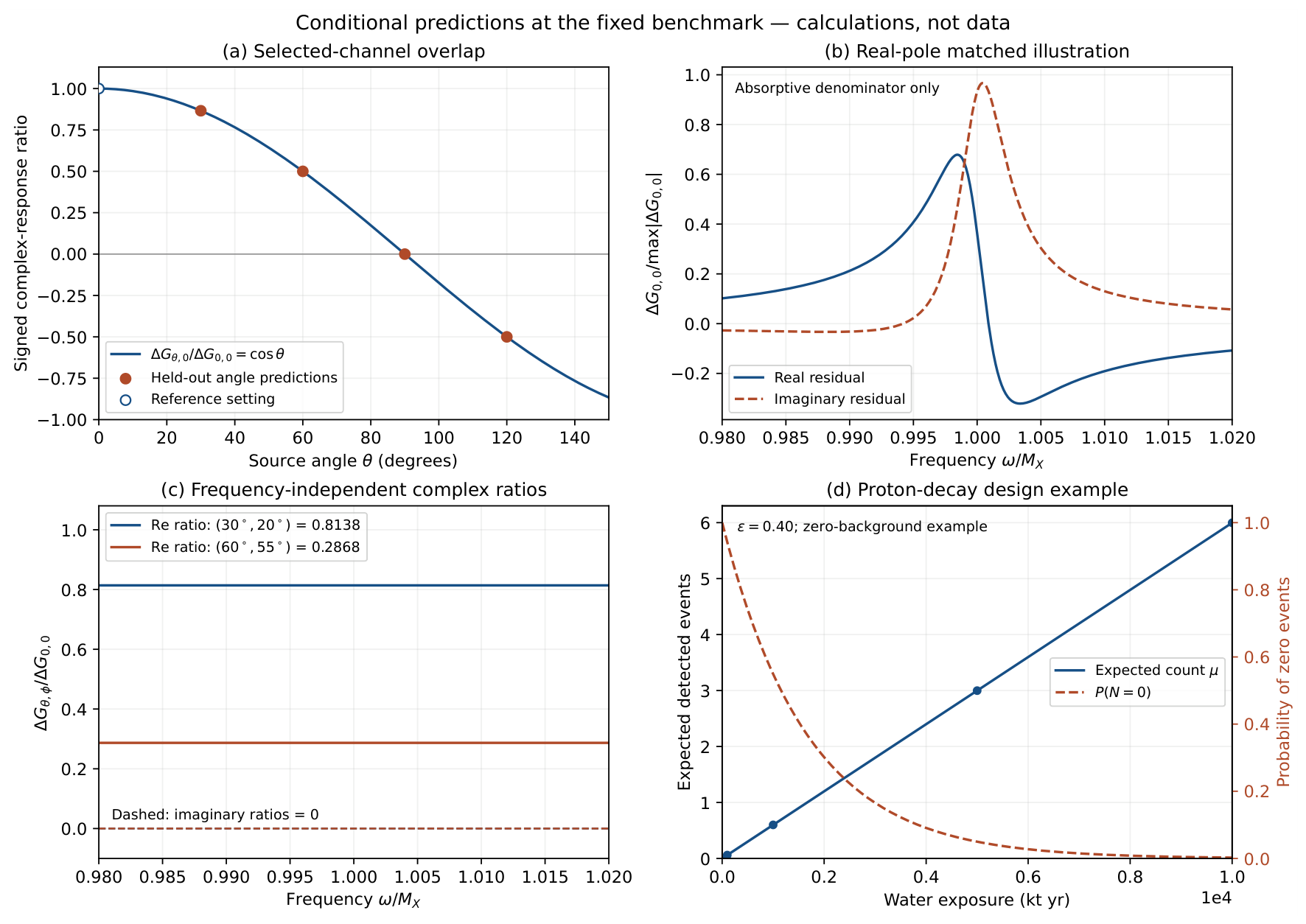
Appendix F Primitive Response Derivatives, Nonuniqueness, and Incompatible Reductions
Appendix F.1. Observation Identity and the Conditions for a Complete Reduction
The quantity Q introduced above is, in the first instance, the mode amplitude of a gauge-invariant field. Identifying it with a coordinate of the primitive observation state s requires the response map of the primitive realization. The primitive variation formula is . If the primitive realization admits a vertical observation direction whose response derivatives satisfy the following relations, that direction induces the corresponding Cauchy data in the transverse channel:
The local expression has mixed curvature , where K is the generator of the original channel. This geometric form defines a primitive observation variation only if the direction belongs to the original admissible domain, preserves the prescribed physical projection, and satisfies the common vacuum response and the remaining constraints. Section 3 verifies these requirements for the realization used in the main construction.
Let denote the mode embedding in the constraint-reduced phase space. The condition for its image to carry the reduced dynamics is
It requires the vector field of the original system to be tangent to the embedded image and to agree there with the equations obtained from the restricted action.
Compatibility of the initial data must persist under evolution. Write for the actual primitive Cauchy-data map, and and for the primitive and parent-field dynamics, respectively. Their dynamical compatibility condition is
If the map depends explicitly on time, must also be included on the left-hand side. The field reduction in the main text verifies mode closure within the parent-field channel; Eq. (A94) instead connects the primitive observation equations to that parent-field evolution. These are distinct requirements. Controlled preparation of a general field mode is conditional on the admissibility and compatibility of the actual map. Section 3 establishes compatibility for the specific realization used here; the conditions for a general map are retained below.
If the actual map at the reference point is , with , pulling back Eq. (12) in its entirety also yields the mixed inertia of the general local model:
Here are derivatives of the actual response map. A coordinate pullback changes the inertia, potential, and curvature together, so their coefficients retain the relations displayed above. The construction in the main text uses , with preparation and readout calculated from that same map.
The closure checked here concerns the selected spatial mode. Whether the remaining matter modes, internal response channels, and metric perturbations also remain closed must be determined from their respective equations. The field–path correspondence therefore requires the original quadratic internal channel to remain invariant, the selected matter mode to be admissible, no unaccounted source to act in the remaining matter directions, and consistent boundary conditions and source normalization throughout. Within this scope, Eqs. (15) and (18) satisfy the original constraints. The actual current profile and the higher-order errors of the nonlinear common action remain to be calculated when this construction is applied to a specific matter system.
Appendix F.2. From Primitive Variations to Transverse Cauchy Data
The primitive observation direction belongs to the original admissible domain; the notation distinguishes it from the spatial mode . Its response is determined by the given connection and projector. Writing q for the variation amplitude along this direction, the corresponding first-order field variation is
The coefficient comes from contraction of the curvature with the observation direction, whereas comes from the covariant variation of the projected subspace. A common frame change has already been eliminated from . Changing the frame therefore cannot adjust the physical restoring force considered below.
For the candidate response selected in Eq. (A92), , , and . Setting gives the field-data map
We retain , , , and . Then and , so the Gauss equation gives . In the original representation containing the orientation coordinate, one may choose , with and . The constrained orientation momentum is therefore not counted again as an independently adjustable initial datum.
Appendix F.3. First-Order Data Sufficient to Determine the Initial Response
The initial canonical field momentum can be calculated from first derivatives of the response. For an actual admissible direction , first-order data near the primitive reference state suffice. Suppose that the response operator has two separated spectral values at the reference state:
This is the spectral-projector variation formula of the unification manuscript in the existing two-block decomposition. Varying determines the off-diagonal blocks, while varying sets the diagonal blocks to zero. The inverse-gap dependence is consistent with the sensitivity of spectral subspaces quantified by classical perturbation bounds [28]. Changes in spectral values are thereby distinguished from changes in subspace orientation: if commutes with , the first-order projector variation in that direction vanishes even when the spectral values change.
For the retained internal generator K, define
Here is the reference spacetime realization. Both the curvature and the projector derivative are first evaluated on the original joint domain and then used along this realization. The internal generator K retains its previous normalization, and . Equation (A99) projects onto the present channel; components in other internal directions remain subject to the existing quadratic closure assumption.
Now let the initial observation displacement vanish identically, and compare only its uniform velocity . Equation (A96) immediately yields
With the initial matter charge held fixed, the Gauss equation requires
Thus the conditions needed for the target transverse initial states reduce to , , and the corresponding admissible velocities . When the initial value is , does not enter Eq. (A100). Recovering the entire transverse history further requires checking , the response profile, and the compatibility condition in Eq. (25).
For the matter-current coupling already retained, the corresponding change in initial acceleration at fixed matter initial data is
The spatial inner product is the one used above, and the second expression compares . At , the terms cancel between and . The expression therefore follows directly from the canonical field momentum and does not omit the initial scalar-potential gradient.
Equations (A98)–(A102) identify two specific geometric quantities that remain to be calculated: the derivative of the response operator between spectral blocks, and the observation–physical mixed curvature of the parent connection. For the present comparison of two initial states, these first-order data determine the initial response. Whether the entire release belongs to the primitive observation evolution is still a question for the actual dynamics.
Appendix F.4. The Dynamical Distinction Between Return Relaxation and Field Oscillation
The return analysis in the unification manuscript goes beyond general structural considerations. Within the three-plus-two block decomposition, it specifies jump operators, stationary occupations, and a coherent-response pairing, including
The second relation assumes the quadratic norm of the coherent response stated in the source. These relations can determine internal dynamical coefficients and can be tested by sequential responses, but they do not specify the spatial mixed components in Eq. (A99). Changing the block occupations is also different from rotating the spectral subspaces, as Eq. (A98) makes explicit.
A more direct constraint follows from the dynamical compatibility proposition in the unification manuscript itself. Near a matched stable equilibrium, the existing adjoint-scalar amplitude and the constant-rate return occupation satisfy, respectively,
Requiring them to remain proportional by a fixed nonzero factor in the same physical time would also imply , and hence . Under the conditions and of the original proposition, nearby nonzero perturbations cannot sustain this identification. The source therefore retains stationary matching while excluding the direct use of independent return relaxation as the instantaneous scalar-amplitude evolution. The same result prevents a calculable return model from being used, without a proven correspondence, as the transverse observation initial state in the present preparation problem.
The final part of the unification manuscript also presents a radial response construction in . The source explicitly treats it as an example of the mechanism, rather than as a substitute for the five-dimensional chiral realization. The present analysis retains the specified five-dimensional internal field and parameters, and determines the required vertical direction through the response realization in Sec. Section 2.
Appendix F.5. A Reference Section Does Not Uniquely Determine the Mixed Curvature
The preceding distinction can be stated as a local proposition. It identifies the supplied data that are insufficient to reconstruct the primitive response, without assuming that every admissible PODA domain is a product.
Proposition
(Local nonuniqueness of reference-section data). Let , and suppose an actual regular patch admits the form , with a projection p preserving the original physical state and reference section . On this patch, take a given local Hermitian bundle, reference connection , response , and its isolated spectral projector . In a fixed trivialization, let K be the existing nonzero anti-Hermitian generator. These reference data alone do not uniquely determine .
Proof.
For any real one-form on , consider
Since and , all these extensions satisfy
Nevertheless, , so
Different choices of therefore give the same reference data and different mixed curvatures. □
Here remains the original physical-state domain throughout. If the reference spacetime realization is , the response that Eq. (A107) induces along spacetime is
One therefore cannot first write an arbitrary spacetime profile as and then claim to have constructed a primitive observation direction. Whether a prescribed profile belongs to the image of also depends on the actual physical-state map and its rank. The proposition uses extensions on the original joint domain and preserves the distinction between physical state and spacetime coordinates.
Nor does nonuniqueness require an entirely invisible observation axis. On a patch admitting two noncollinear one-forms, one may choose two nonzero, noncollinear values of . When the corresponding comparison loops are admissible, both extensions have nontrivial mixed transport. Comparisons along different physical directions distinguish them; a vanishing response in one readout does not deprive the entire observation axis of its behavioral identity. If the complete primitive path transport is already supplied as input, these two extensions no longer share the same given data, and that input removes the nonuniqueness.
The proposition preserves the same reference background, internal generator, and masses and couplings in the parent action. It does not assert that the primitive actions obtained by pulling back different extensions are identical, nor does it establish that all such extensions satisfy every primitive admissibility and preparation condition. Its precise conclusion is that a reference section and its parent-field equations do not uniquely select the mixed curvature. The local realization in the main text selects one extension by specifying the complete transport, and then verifies its observation identity and dynamical compatibility separately.
Appendix F.6. Matter Responses to Different Mixed Curvatures
The distinction has consequences beyond the formal expressions. Retain the periodic spatial domain, unit transverse area, and wavenumber . The original vector field already possesses two orthogonal transverse polarizations:
Both have unit spatial norm, zero divergence, and satisfy . They are existing spatial polarizations of the same internal K channel and introduce no new field or mass. To avoid confusion with the physical state, denotes only a spatial Cartesian basis vector here.
If a primitive realization separately admits , Eq. (A100) gives two families of field initial states:
Even without this assumption about the primitive realization, these are valid parent-field initial states: both families satisfy the Gauss constraint, and each initial state has energy . With the same matter-current profile fixed in both cases,
The same reference field, initial-state energy, and field constraints are therefore insufficient to determine the response of the selected readout. The difference is determined by the polarization into which the primitive variation enters and its overlap with the matter current.
To check the conclusion after release, the numerical calculation retains both polarizations and the matter coordinate throughout, giving six first-order state variables governed by
These equations follow directly by orthogonal projection of the same quadratic parent field. For the comparison in the present preparation problem, with and the common external source , the first family reproduces Eq. (47); the second has and a free transverse oscillation. An additional matter drive would also excite the first polarization. This example therefore does not establish that the one-dimensional image of the second polarization is closed under arbitrary driving.
Appendix F.7. Incompatibility of a Constant-Potential Path with a Massive Field Mode
Keeping the same , consider the path evolution obtained by deleting the field restoring term. This comparison tests whether the two sets of equations correspond; it does not introduce a separate set of physical parameters. Denoting the truncated vector field by gives
If as well, this reduces to the constant-potential path branch without mixed inertia of the local action in Eq. (A2). Whenever , its residual in the parent-field equation is . Since the original channel has , even the spatially constant mode gives ; the long-wavelength limit cannot remove this term exactly.
The case with is easier to overlook. The initial Gauss constraint is then satisfied, and Eq. (A113) vanishes momentarily, but
Agreement of the instantaneous velocities at one initial point does not imply that the two systems subsequently follow the same curve. Satisfying both sets of equations over a time interval requires ; when , it also requires . Histories common to the two systems under these conditions therefore cannot describe release with a nonzero observation velocity.
The coordinate mixing introduced above cannot remove this difference. For an admissible coordinate change preserving the physical projection, , the pullback of the original potential contains
At the reference equilibrium, second-order terms in a nonlinear coordinate change likewise cannot alter this nonzero quadratic form in the vertical direction, because the first derivative of the original potential vanishes there. This excludes direct identification of the field branch with the constant-potential path branch while preserving the physical projection, time, and original action. The two variational realizations in PODA retain their respective equations; the calculation identifies the difference that must be kept when relating them.
Appendix F.8. Longitudinal Release Cannot Replace Transverse Preparation
Another constraint-satisfying set of parent-field data is , , and . These data satisfy the initial constraints and produce a longitudinal response after release. Two issues must be distinguished.
First, if the condition , corresponding to variation only in the projector direction, is imposed on the entire history, Eq. (A96) gives , and hence and . The two initial matter currents are the same, yet the common field equation at the stated initial data requires
A nontrivial gradient causes the parent-field evolution to leave this forcibly restricted image immediately. If and are maintained throughout a neighborhood, the full equation more directly requires . This does not exclude the release solution in the source: that solution permits the connection to evolve after preparation, and this evolution produces the subsequent canonical field momentum.
Second, even a valid longitudinal release solution does not excite the transverse matter mode selected in this section. Within the same isotropic quadratic kernel, the difference in transverse fields and the matter coordinate form a closed homogeneous subsystem. Their initial data and external-source difference are zero, and the longitudinal component does not enter the subsystem. Uniqueness of the initial-value problem then keeps both the transverse-field difference and the matter-motion difference at zero. For periodic or decaying boundary conditions, the remaining longitudinal canonical field momentum is orthogonal to , so the conclusion can also be checked directly from the original force expression:
The initial conditions therefore give . The common transverse part produced by the same external source cancels in the difference between the two cases. This conclusion concerns the transverse current and readout selected here; it does not imply that longitudinal responses are invisible to all matter. It specifically excludes substituting the longitudinal release example in the source for Eq. (44).
Appendix F.9. Numerical Verification of the Existing Examples
The numerical checks use the same synthetic coefficients as the main text: , , , , , and . The program checks Eq. (47) by independent ordinary-differential-equation integration, reconstructs the spatial field, and verifies the Gauss constraint, field equations, matter feedback, and energy. It also computes the nonzero residual of the truncated equations and the zero longitudinal readout response. Figure A8 shows these distinctions. The synthetic coefficients serve to verify the equations and algorithms; they are not used to estimate the scales of the high-energy benchmark.
For this example, , , , and . The maximum absolute difference between the analytic displacement and the independent integration is , and the residual of the full spatial field equation is below . The fourth-derivative difference in the truncated calculation is exactly . These numerical errors test the implementation of the equations; they do not quantify quantum or nonlinear errors in the original theory.
Figure A8.
Compatibility and release calculations with the stated synthetic coefficients. The analytic curves and independent integration check the complete response of the two initial states. Deleting the restoring force leaves the initial acceleration unchanged but produces a trajectory that departs from the common field evolution and has a nonzero field residual. Longitudinal release can have nonzero canonical field momentum while its projection onto the selected transverse matter mode vanishes. All curves are theoretical calculations within the same quadratic model.
Figure A8.
Compatibility and release calculations with the stated synthetic coefficients. The analytic curves and independent integration check the complete response of the two initial states. Deleting the restoring force leaves the initial acceleration unchanged but produces a trajectory that departs from the common field evolution and has a nonzero field residual. Longitudinal release can have nonzero canonical field momentum while its projection onto the selected transverse matter mode vanishes. All curves are theoretical calculations within the same quadratic model.
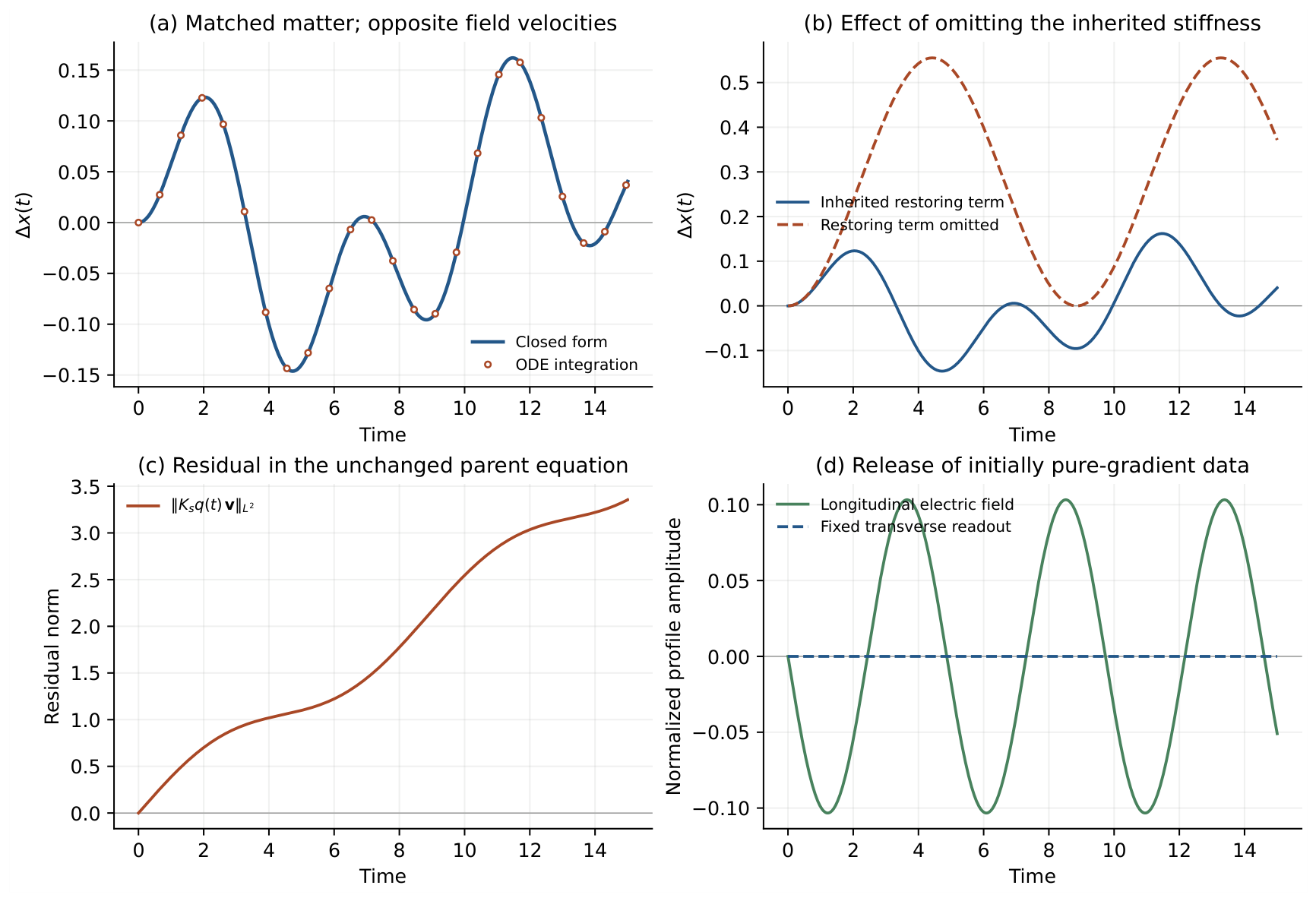
Appendix F.10. Numerical Verification of the Two Polarizations
The calculation again uses the same synthetic coefficients: , , , , , , and . Each initial state in either polarization family has energy . The paired initial-acceleration differences are and 0, respectively, and the displacement differences at are and 0. The Gauss equation and current continuity hold identically. The equation residual of the reconstructed parent field is below , and the maximum difference between independent integration and the matrix exponential is below .
The program also checks the spectral-projector derivative in the original three-plus-two decomposition and computes mixed-loop transport for two nonzero connection extensions. The best absolute error for the derivative in the bridge direction is ; the corresponding error for a general Hermitian perturbation is . These numerical checks verify analytic relations and do not measure the accuracy of a physical approximation. Figure A9 presents the spectral projector, mixed transport, and matter response within the same verification.
Figure A9.
Verification of first-order primitive response data and the existing parent-field initial states. Top left: finite-difference error in the spectral-projector derivative; the projector derivative of a commuting spectral perturbation is exactly zero. Top right: transport coefficients of two formal extensions on different mixed rectangles, with nonzero comparisons for each extension. Bottom left: equal-energy initial states and their initial matter responses. Bottom right: the displacement difference between the two releases. The loop calculation uses ; the plotted mixed-curvature coefficients are extracted with this orientation. All panels show theoretical calculations of the responses of different polarizations under the same matter readout.
Figure A9.
Verification of first-order primitive response data and the existing parent-field initial states. Top left: finite-difference error in the spectral-projector derivative; the projector derivative of a commuting spectral perturbation is exactly zero. Top right: transport coefficients of two formal extensions on different mixed rectangles, with nonzero comparisons for each extension. Bottom left: equal-energy initial states and their initial matter responses. Bottom right: the displacement difference between the two releases. The loop calculation uses ; the plotted mixed-curvature coefficients are extracted with this orientation. All panels show theoretical calculations of the responses of different polarizations under the same matter readout.
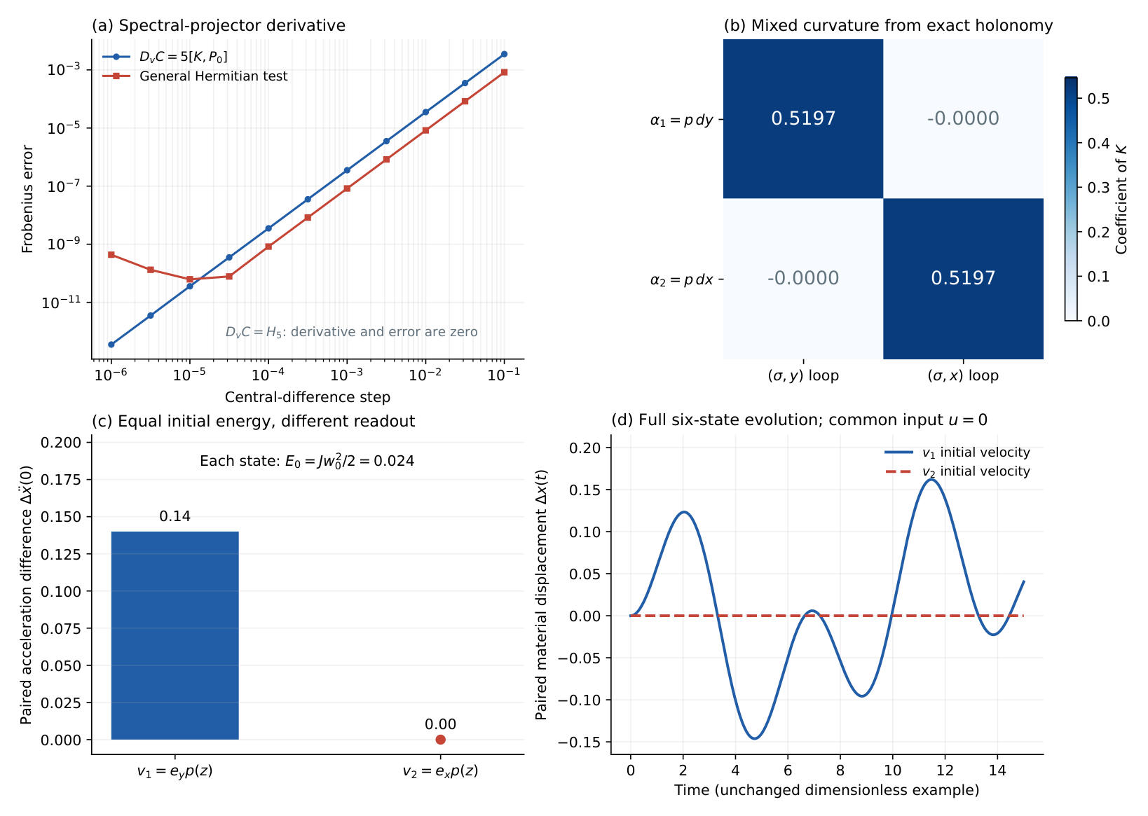
References
- Meng, X. A Categorical Reconstruction of Meta-Laws: A Philosophical Perspective on the M-L-O Structure. Preprints (2026) 202609 2015, 1. [CrossRef]
- Meng, X. A Set-Theoretic Derivation of Physobser Axiom: Irreducibility, Minimality, and Essential Uniqueness of the Physical–Observation Dual-Axis Structure. Preprints (2026) 202608.1046, Version 2. [CrossRef]
- Meng, X. A Categorical Derivation of Physobser Axiom: Irreducibility, Minimality, and Essential Uniqueness of the Physical–Observation Dual-Axis Structure. Preprints (2026) 2, 202608.1298. [CrossRef]
- Meng, X. The Natural Dual-Axis Structure of Observation: Categorical Foundations and Consequences for Quantum Theory. Preprints (2026) 3, 202609.0572. [CrossRef]
- Meng, X. The Phase Transport Fundamental Equation on the Physical–Observation Dual-Axis Structure. Preprints (2026) version 2, 202608.1128. [CrossRef]
- Meng, X. Unification of the Four Interactions in PODA Observation Geometry: Common Dynamics, Gravity–Gauge Coupling, and Quantum Consistency. Preprints (2026) 1, 202609.2408. [CrossRef]
- Kalman, R. E. On the general theory of control systems. IFAC Proc. Vol. 1960, 1(1), 491–502. [Google Scholar] [CrossRef]
- Ho, B. L.; Kalman, R. E. Effective construction of linear state-variable models from input/output functions. Regelungstechnik 1966, 14, 545–548. [Google Scholar] [CrossRef]
- Bellman, R.; Åström, K. J. On structural identifiability. Math. Biosci. 1970, 7, 329–339. [Google Scholar] [CrossRef]
- Berry, M. V. Quantal phase factors accompanying adiabatic changes. Proc. R. Soc. Lond. A 1984, 392, 45–57. [Google Scholar] [CrossRef]
- Simon, B. Holonomy, the quantum adiabatic theorem, and Berry’s phase. Phys. Rev. Lett. 1983, 51, 2167–2170. [Google Scholar] [CrossRef]
- Wilczek, F.; Zee, A. Appearance of gauge structure in simple dynamical systems. Phys. Rev. Lett. 1984, 52, 2111–2114. [Google Scholar] [CrossRef]
- Higham, N. J. Computing the polar decomposition—with applications. SIAM J. Sci. Stat. Comput. 1986, 7, 1160–1174. [Google Scholar] [CrossRef]
- Schreiber, U.; Waldorf, K. Parallel transport and functors. J. Homotopy Relat. Struct. 2009, arXiv:0705.04524(1), 187–244. [Google Scholar] [CrossRef]
- Dirac, P. A. M. Generalized Hamiltonian dynamics. Can. J. Math. 1950, 2, 129–148. [Google Scholar] [CrossRef]
- Faddeev, L.; Jackiw, R. Hamiltonian reduction of unconstrained and constrained systems. Phys. Rev. Lett. 1988, 60, 1692–1694. [Google Scholar] [CrossRef]
- Hermann, R.; Krener, A. J. Nonlinear controllability and observability. IEEE Trans. Autom. Control 1977, 22(5), 728–740. [Google Scholar] [CrossRef]
- Kubo, R. Statistical-mechanical theory of irreversible processes. I. General theory and simple applications to magnetic and conduction problems. J. Phys. Soc. Jpn. 1957, 12, 570–586. [Google Scholar] [CrossRef]
- Ward, J. C. An identity in quantum electrodynamics. Phys. Rev. 1950, 78, 182. [Google Scholar] [CrossRef]
- Aoyama, T.; Hayakawa, M.; Kinoshita, T.; Nio, M. Proper Eighth-Order Vacuum-Polarization Function and its Contribution to the Tenth-Order Lepton g-2. Phys. Rev. D. 2011, arXiv:1012.5569v383, 053003. [Google Scholar] [CrossRef]
- Beneke, M. Unstable-particle effective field theory. Nucl. Part. Phys. Proc. 2015, arXiv:1501.07370261–262, 218–231. [Google Scholar] [CrossRef]
- Cowan, G.; Cranmer, K.; Gross, E.; Vitells, O. Asymptotic formulae for likelihood-based tests of new physics. Eur. Phys. J. C 2011, 71, 1554. [Google Scholar] [CrossRef]
- CERN. The Large Hadron Collider. Official facility description; proton collision energy 13.6TeV. 5 October 2026. Available online: https://home.cern/science/accelerators/large-hadron-collider/.
- Appelquist, T.; Carazzone, J. Infrared singularities and massive fields. Phys. Rev. D. 1975, 11, 2856–2861. [Google Scholar] [CrossRef]
- Aoki, Y.; Izubuchi, T.; Shintani, E.; Soni, A. Improved lattice computation of proton decay matrix elements. Phys. Rev. D. 2017, 96, 014506. [Google Scholar] [CrossRef]
- Yoo, J.-S.; Aoki, Y.; Boyle, P.; Izubuchi, T.; Soni, A.; Syritsyn, S. Proton decay matrix elements on the lattice at physical pion mass. Phys. Rev. D. 2022, 105, 074501. [Google Scholar] [CrossRef]
- A. Takenaka et al. (Super-Kamiokande Collaboration); et al. Search for proton decay via p→e+π0 and p→μ+π0 with an enlarged fiducial volume in Super-Kamiokande I–IV. Phys. Rev. D. 2020, arXiv:2010.16098v2102, 112011. Available online: https://arxiv.org/abs/2010.16098. [CrossRef]
- Davis, C.; Kahan, W. M. The rotation of eigenvectors by a perturbation. III. SIAM J. Numer. Anal. 1970, 7(1), 1–46. [Google Scholar] [CrossRef]
Figure 1.
Explicit preparation and release within the same quadratic common action. The two inputs have opposite signs and both vanish continuously before release. The matter position and velocity return to identical values, while the observation velocities retain opposite signs. Cumulative input work agrees with the joint stored energy, and the subsequent displacement difference follows Eq. (41). The parameters are the synthetic verification set given in the text; all curves are theoretical calculations.
Figure 1.
Explicit preparation and release within the same quadratic common action. The two inputs have opposite signs and both vanish continuously before release. The matter position and velocity return to identical values, while the observation velocities retain opposite signs. Cumulative input work agrees with the joint stored energy, and the subsequent displacement difference follows Eq. (41). The parameters are the synthetic verification set given in the text; all curves are theoretical calculations.
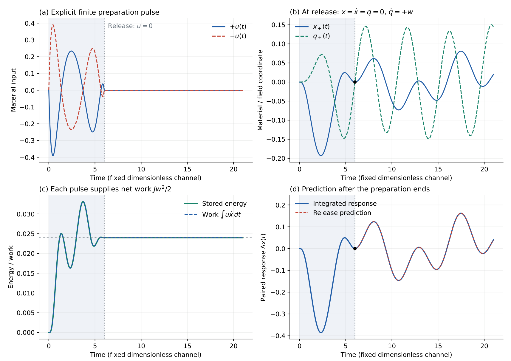
Figure 2.
Primitive comparison and matter records for the same release process. Left: the two comparison probabilities, calculated from a fixed vector, effect, and path in the existing five-dimensional response. Right: independent calculations of the two sides of Eq. (51), verifying their correspondence on the selected inverse branch. The path geometry and dynamical parameters are identical for both preparations, without refitting the release records.
Figure 2.
Primitive comparison and matter records for the same release process. Left: the two comparison probabilities, calculated from a fixed vector, effect, and path in the existing five-dimensional response. Right: independent calculations of the two sides of Eq. (51), verifying their correspondence on the selected inverse branch. The path geometry and dynamical parameters are identical for both preparations, without refitting the release records.
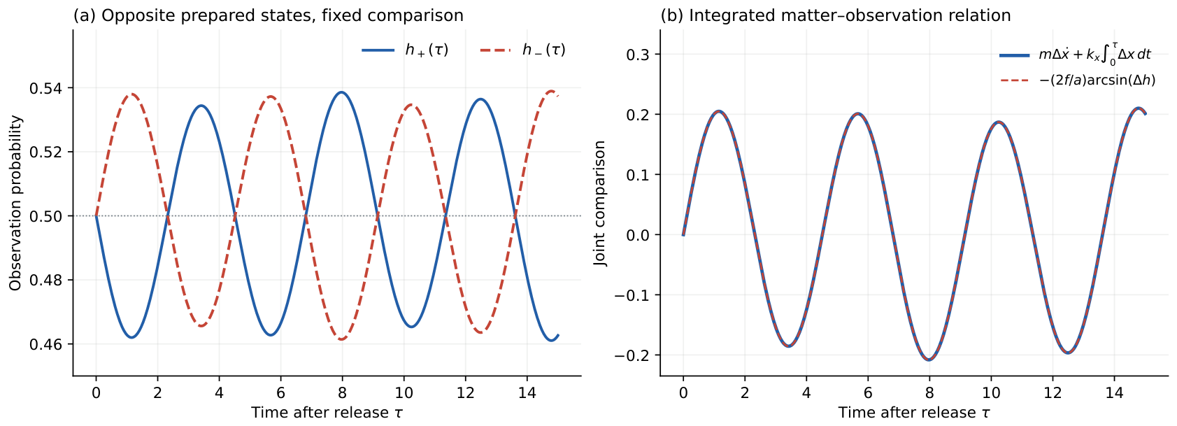
Disclaimer/Publisher’s Note: The statements, opinions and data contained in all publications are solely those of the individual author(s) and contributor(s) and not of MDPI and/or the editor(s). MDPI and/or the editor(s) disclaim responsibility for any injury to people or property resulting from any ideas, methods, instructions or products referred to in the content. |
© 2026 by the authors. Licensee MDPI, Basel, Switzerland. This article is an open access article distributed under the terms and conditions of the Creative Commons Attribution (CC BY) license (http://creativecommons.org/licenses/by/4.0/).
Copyright: This open access article is published under a Creative Commons CC BY 4.0 license, which permit the free download, distribution, and reuse, provided that the author and preprint are cited in any reuse.