

Submitted:
03 October 2026
Posted:
08 October 2026
You are already at the latest version
Abstract
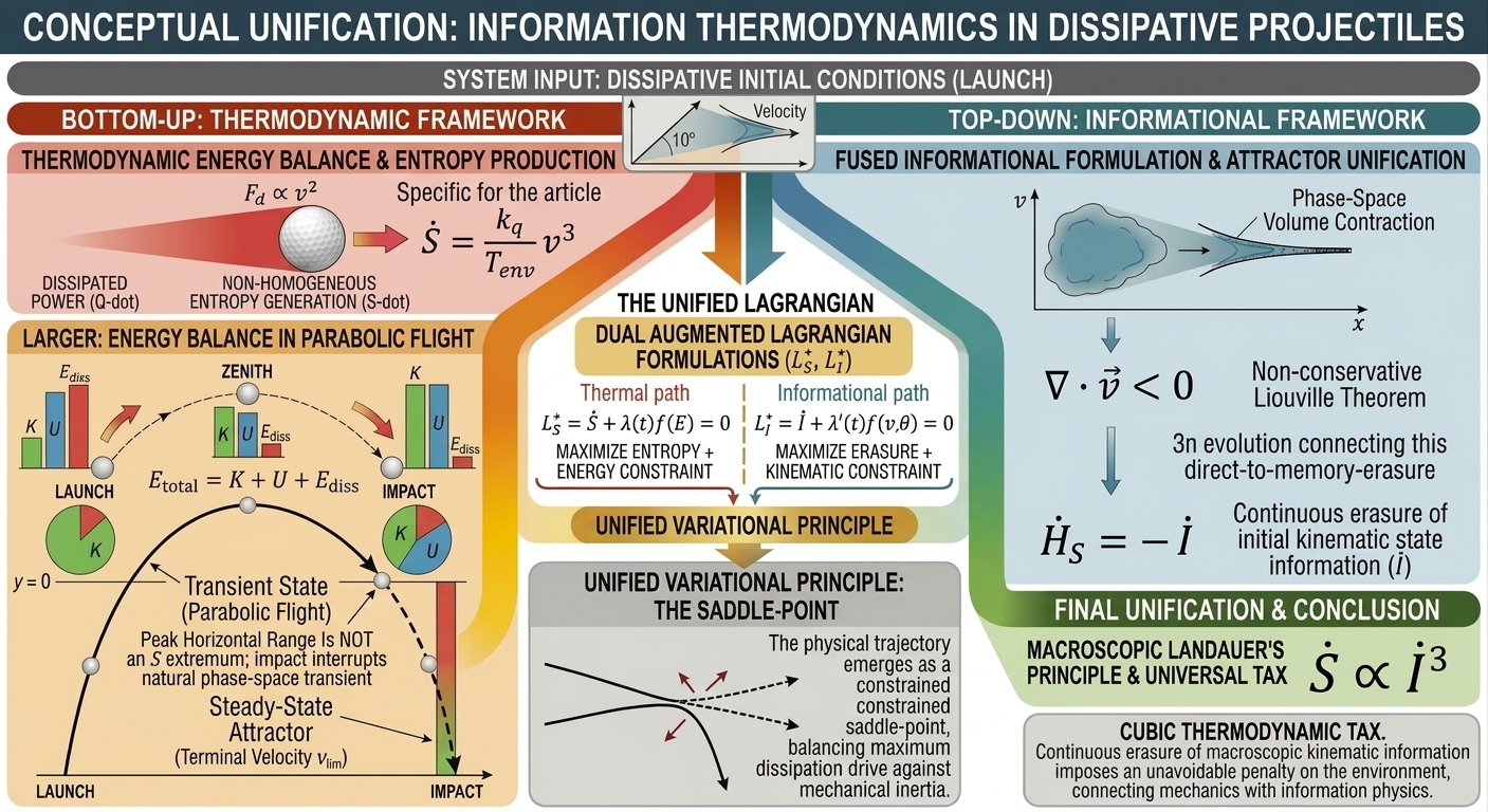
This paper reinterprets the mechanics of projectile motion with quadratic aerodynamic drag through the lens of non-equilibrium thermodynamics and information theory. Rather than treating aerodynamic drag merely as mechanical energy loss, we develop dual augmented Lagrangians (L_S^* and L_I^*) that unify macroscopic energy and entropy balances within a single variational framework. By reformulating the system in both thermodynamic and purely informational terms, a conceptual duality is established. The resulting variational saddle-point represents a dynamic compromise: it balances the natural drive to rapidly erase the system's initial kinematic state against the intrinsic mechanical and thermodynamic inertia that resists instantaneous dissipation.
Applying this framework, analytical results reveal that the classical bounded parabolic flight is fundamentally an incomplete thermodynamic transient. Entropy production is non-homogeneous throughout the trajectory, as we find that the optimal launch angle for maximum horizontal range does not correspond to a global thermodynamic extremum. Instead, this geometric optimum is a parametric artefact forced by the ground impact, which arbitrarily truncates the system's natural phase-space evolution toward its steady-state attractor, the terminal velocity.
Ultimately, this framework proves that the continuous phase-space contraction and erasure of macroscopic kinematic information imposes an unavoidable cubic thermodynamic tax on the environment. By explicitly correlating mechanical dissipation with informational loss, we establish a firm macroscopic connection between classical mechanics, non-equilibrium thermodynamics, and the physics of information.
Keywords:
entropy
; dissipative systems
; variational methods
; information entropy
; coupled thermomechanical system
; attractor
1. Introduction
Variational principles, such as the Principle of Stationary Action, are foundational to modern physics, describing the evolution of conservative systems through Lagrangian and Hamiltonian formalisms. Standard classical approaches to dissipative mechanical systems typically treat non-conservative forces either phenomenologically, such as through the introduction of Rayleigh dissipation functions to maintain the Lagrangian formalism [1], or via external work-energy balances [2]. More recently, Unified Mechanics Theory has sought to integrate thermodynamics directly into continuum mechanics to model material degradation and fatigue in solid systems [3].
Dissipation is intrinsically linked to entropy generation in non-equilibrium thermodynamics [4,5]. Historically, classical frameworks established that isolated systems evolve toward equilibrium states that maximise entropy [6,7,8]. Seeking to describe non-equilibrium processes, Prigogine pioneered the Minimum Entropy Production Principle (MEPP). However, as Jaynes [9] and Landauer [10] noted, the validity of MEPP is generally restricted to linear regimes near equilibrium. Beyond these linear regimes, the exact role of entropy in macroscopic continuous dynamics remains historically contentious, often leading to theoretical misconceptions regarding whether real systems minimise or maximise dissipation [11], or prompting various Maximum Entropy Production approaches [7,8]. Addressing this duality, Lucia recently emphasised that whether an actual physical trajectory minimises or maximises entropy generation strongly depends on the choice of system boundaries and the specific dynamic constraints applied [12]. Building upon these foundational debates, thermodynamic optimization and advanced non-equilibrium formalisms have developed a rich history, exemplified by frameworks such as Bejan's entropy generation minimization [13] and Jou’s extended irreversible thermodynamics [14].
Concurrently, modern non-equilibrium statistical mechanics has established robust mathematical connections between non-conservative phase-space dynamics, Shannon entropy [15], and thermodynamic dissipation [16]. A cornerstone of this relationship is Landauer's principle [17], which posits that the logical or physical erasure of information inherently requires a minimum thermodynamic cost in the form of heat dissipated to the environment. This thermodynamics of information has been validated primarily in microscopic stochastic systems and computing networks [18].
Despite these independent advances across mechanics, thermodynamics, and information theory, a significant gap persists: formulating these principles into a strict variational calculus framework—where macroscopic continuous dissipation is embedded directly into a purely geometric entropic action—remains a theoretical challenge. Macroscopic projectile motion subject to quadratic aerodynamic drag provides an ideal, highly transient physical paradigm to confront this open problem. While traditional Newtonian mechanics successfully predicts the geometric trajectory, it treats air resistance merely as a phenomenological mechanical loss. This classical perspective offers limited insight into the underlying thermodynamic and informational nature of the flight as it evolves toward a steady-state dynamical attractor, i.e., the terminal velocity [1].
In this contribution, we reinterpret dissipative macroscopic mechanics through the unified lens of non-equilibrium thermodynamics and information theory. We propose that because a dissipative projectile undergoes a continuous, irreversible contraction of its kinematic phase space toward a singular terminal attractor, it is mathematically erasing its initial state information. This reveals a coupling where macroscopic aerodynamic drag can be understood through information theory: the continuous erasure of initial mechanical conditions exacts an inevitable thermodynamic cost. Following the variational methodology described in Feynman’s Lectures on Physics for the minimum action principle [19], we construct an extended Lagrangian where the fundamental variable of optimization is entropy rather than action. By setting Newtonian dynamics as a geometric constraint on the environment's natural tendency to maximise entropy production, we demonstrate that the resulting trajectory emerges as a singular saddle-point extremal. Ultimately, this framework establishes a conceptual duality between continuous kinematic information loss and physical heat dissipation, proving that classical mechanical drag inherently acts as the physical penalty for the continuous erasure of macroscopic information.
The remainder of this paper is organised as follows. Section 2 establishes the physical framework, defining the macroscopic energy balances and the thermodynamic boundaries of the coupled system. Section 3 develops the entropy variational formulation, introducing the augmented Lagrangian and demonstrating the Hamiltonian nature of the singular extremal. Section 4 formulates the dynamics in terms of information theory, linking the phase-space contraction to the continuous loss of kinematic information. Section 5 presents the numerical simulation results, illustrating both the asymptotic convergence to the steady-state attractor and the optimization of the transient parabolic flight.Section 6 discusses the conceptual implications of the unified Lagrangian and outlines the limitations of the model, while Section 7 provides the concluding remarks. Finally, the supplementary appendices provide the rigorous mathematical derivations supporting this framework, including the equations of motion in intrinsic coordinates (Appendix A), the detailed variational calculus (Appendix B), the Liouville-Shannon phase-space formulation (Appendix C), the entropy equations for the constant impact range scenario (Appendix D), an extension to the linear friction regime (Appendix E), and the generalised entropy Lagrangian formulation for continuous dissipative systems (Appendix F)..
2. The Physical Framework of Projectile Motion
To construct a thermodynamic model of projectile motion, we must first reframe the mechanical dissipative flight as a macroscopic, closed, non-isolated system coupled to an isothermal environment. This requires defining the thermal boundaries and characterising the non-equilibrium transient states the projectile traverses during its flight. In this section, we establish the fundamental kinematic constraints governing the dissipative trajectory and formulate the instantaneous entropy production rate. By analysing the macroscopic heat dissipation, we lay the groundwork to link the mechanical properties of the flight to the thermodynamic evolution of the system, setting the stage for the variational approach.
2.1. Classical Mechanics and the Macroscopic Energy Balance
Macroscopic projectile motion involves continuous energy dissipation, which breaks the geometric symmetry of idealised parabolic flight (as illustrated in Figure 1a). While low-speed microscopic particles (low Reynolds number) experience linear drag, macroscopic objects at higher speeds are modelled by quadratic aerodynamic drag [20]:
This non-conservative force continuously dissipates mechanical energy into the environment, shortening the maximum range across different launch angles (Figure 1b). From a mechanical perspective, this dissipative motion is governed by an energy balance among kinetic energy (K), potential energy (U), and the heat dissipated along the path (Q), expressed as:
where m is the mass, h the height, g the gravity acceleration, and l represents the path over which the energy dissipation occurs. While these standard mechanical frameworks successfully predict the motion of projectiles [21,22], our approach shifts the analysis from a traditional force-based description to an energy-based thermodynamic perspective. To build this variational framework, we first explicitly define the thermodynamic states and the thermal boundaries of the coupled system.
2.2. Thermodynamic System and States
We define the projectile and the surrounding air as a coupled thermomechanical system, as illustrated in Figure 2. The interaction between the solid body and the fluid is characterised by the aerodynamic drag coefficient, k. In non-equilibrium thermodynamics, it is critical to define the thermal boundary conditions. Here, we model the surrounding atmosphere as an infinite, isothermal heat bath at a constant temperature T. For macroscopic projectiles traveling at subsonic speeds, the aerodynamic heating of the solid body itself is negligible. Consequently, all the mechanical power dissipated by the drag force
is entirely transferred as convective heat to the environment. This physical assumption allows us to define the instantaneous macroscopic entropy production rate as:
A comprehensive thermodynamic description requires defining the state of the system. In standard equilibrium thermodynamics, a state is well-defined when macroscopic variables remain time-invariant. During the projectile’s flight, however, both speed and angle evolve continuously, placing the system in a transient, non-equilibrium state. Unlike conservative systems, dissipative trajectories lack time-reversal symmetry and continuously lose mechanical energy. If the projectile undergoes an unconstrained fall, this continuous dissipation eventually balances the gravitational force, driving the system toward a macroscopic steady state where it reaches terminal velocity,
which is completely independent of the initial launch conditions. Consequently, this terminal state acts as a dynamical attractor in phase space. Because distinct trajectories continuously converge toward this attractor, the system’s phase-space volume contracts over time. From an information-theoretic perspective, this continuous phase-space contraction means that the system gradually loses memory of its initial kinematic state, resulting in a continuous erasure of initial condition information.
2.3. The Entropy Variational Formulation
Having established the continuous loss of kinematic information, we now seek the fundamental physical principle governing this path. By defining an entropy-based Lagrangian, we use variational calculus to find the feasible physical trajectories.
2.3.1. The Thermodynamic Entropy Functional
Starting from the instantaneous entropy production rate , the total entropy generated throughout the flight path is evaluated by integrating over time. To express the trajectory directly within the geometric domain, this time integration is transformed into the path-angle differential dθ, using the kinematic relations detailed in Appendix A. The total thermodynamic entropy functional is expressed as (detailed in Appendix B.1):
where the integrand acts as our unconstrained Entropy Lagrangian,
However, this unconstrained expression yields non-physical trajectories. As demonstrated in Appendix B.1, unconstrained optimization of this functional forces the tangential acceleration to be zero, restricting the system to a steady-state regime. Therefore, physical kinematic constraints must be introduced. Applying Newton’s second law in intrinsic coordinates (tangential and normal axes), we derive the constraint coupling velocity v, the angle θ, and the derivative of the velocity with respect to the angle, v'(dθ) = dv/dθ. As derived in Appendix B.2, this constraint can be written as G(v, v’, θ) = 0, where:
To extremise the total entropy subject to this kinematic restriction, we introduce a trajectory-dependent Lagrange multiplier, λ(θ) ). This multiplier acts as a local thermodynamic entropy potential, representing the thermodynamic cost of enforcing the Newtonian path. The augmented Lagrangian, *(v,v',θ,λ), takes the form:
Applying the Euler-Lagrange equation to * with respect to velocity v:
yields the differential equation governing the evolution of. The stationary trajectory (dS = 0) requires:
where λ'(θ) = dλ/dθ. This result shows that the evolution of the Newtonian trajectory is coupled to the thermodynamic cost of adhering to the dynamic geometric constraint. Here, λ(θ) can be interpreted as an entropic sensitivity factor quantifying the response of the entropy production rate to the kinematic drag constraint [14].
2.3.2. The Hamiltonian Nature of the Extremal
The generalised momentum corresponding to our spatial evolution variable q is defined as . Applying the Legendre transformation, the Hamiltonian is given by H = v’ p - *. Substituting our previous expressions (as detailed in Appendix B.4), the Hamiltonian evaluates to:
To determine the nature of this extremal, we evaluate the second variation of the entropy functional (the Legendre condition) and find that it vanishes identically (d2S = 0). In variational calculus, this vanishing second variation defines the trajectory as a singular extremal, representing a functional saddle point in entropy space. Physically, this implies that the trajectory balances the thermodynamic tendency to maximise entropy production with the rigid kinematic boundaries imposed by classical mechanics.
Subject to Newtonian constraints, the trajectory for any launch angle is characterised by maximum allowable energy dissipation and maximum entropy generation. This contrasts with the Principle of Least Action in non-dissipative systems. While the standard mechanical action balances kinetic and potential energies to find a minimum, the unconstrained entropic Lagrangian lacks this internal stabilization. As previously demonstrated by the naïve Lagrangian (9), attempting to optimise entropy without restrictions yields non-physical solutions. Imposing Newton's laws as a dynamic constraint yields the saddle point, ensuring the trajectory dissipates the maximum energy permitted by the geometric boundaries.
2.3.3. The Geometric Evolution of Entropy Production
A consequence of the variational framework is the dependence of the thermodynamic entropy production on the trajectory’s geometry. By substituting the analytical solution of the velocity profile into the entropy production rate equation (), the entropy generation can be formulated purely in terms of the instantaneous path angle q (as derived via the energy domain in Appendix A.4):
Where a is the initial launch angle, v0 is the initial velocity, vt is the terminal velocity, and F(q) is a geometric function defined as:
This formulation maps the instantaneous entropy production rate directly onto the angular evolution of the path. Integrating this rate yields the total accumulated entropy. The dependence on F(q) reflects a non-linear entropy production during thces the vertical asymptote ( -90º) and the velocity converges to vt, the entropy production rate stabilises at a constant terminal value (). This formulation characterises the system's transition from an initial transient state to a steady dissipation profile.
2.4. The Information Framework and Information Loss
The convergence towards the terminal velocity is governed by a dynamic attractor. As shown in Figure 3, regardless of the initial launch conditions, the system’s phase space contracts toward this final state. This convergence implies a continuous loss of the system’s initial kinematic information.
To formalise this information loss, we evaluate the divergence of the state velocity field in the velocity phase space. Using the Liouville equation for a dissipative 2D system governed by quadratic drag, the rate of change of the continuous Shannon entropy (HS) associated with the kinematic probability distribution is (see Appendix C for the full derivation) [23]:
Where a is the acceleration. Shannon entropy decreases as the phase space contracts. We define the rate of kinematic information lost by the system, , as the negative change in Shannon entropy:
Integrating this expression reveals that the total information lost by the system is proportional to the physical path length l(t) travelled by the projectile:
In this framework, the terminal velocity attractor acts as an entropic potential well. The divergence of the velocity field drives a flow of microstates through phase space until the initial kinematic information is dissipated and the system settles into its macroscopic steady state.
By combining the entropy production rate (6) with the information loss rate (), we find the relationship:
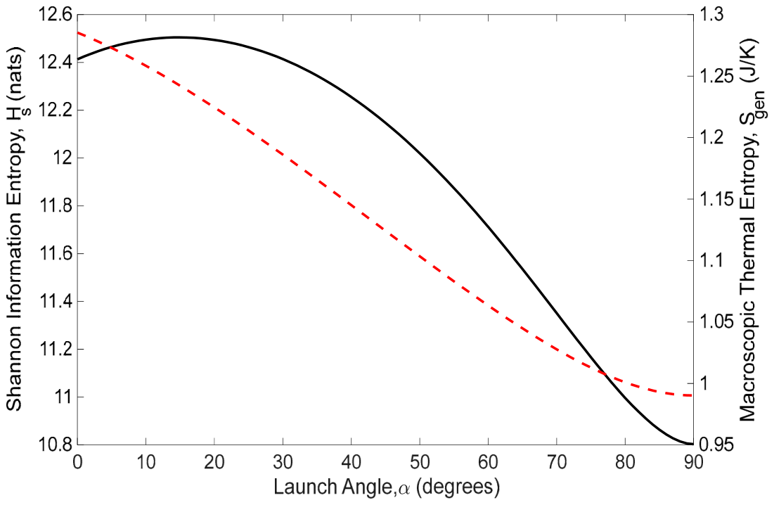
This cubic dependency demonstrates that dissipating thermodynamic heat into the environment is coupled to the loss of the system's initial kinematic information as it converges toward the attractor.
3. Simulation Results of the Model
The theoretical trajectories derived from the variational framework were evaluated using the physical parameters of a standard golf ball: mass of m = 45.93 g, diameter d = 4.267 cm, and a quadratic drag coefficient k = 2.1·10-4 kg/m. Numerical simulations and curve fitting were performed in MATLAB. Code generation and mathematical verification were assisted by the Gemini 3.1 Pro large language model.
3.1. Thermodynamic Entropy and Information Evolution Towards the Steady State
The evolution of thermodynamic entropy production as a function of position as the system approaches the macroscopic steady state (terminal velocity) is illustrated in Figure 4a, as inferred from (15). The continuous loss of kinematic information during the flight, driven by energy dissipation, is depicted in Figure 4b, generated using (19). Because the terminal state is an asymptotic limit, numerical simulations were truncated when the projectile reached 99.9% of its theoretical terminal velocity.
The steady-state behaviour of the system is captured by evaluating the governing differential equation for λ(θ) (13) in its asymptotic limit. As the trajectory approaches the vertical asymptote (q →-90º) and the velocity converges to the terminal attractor (v→ vt), the dynamic Lagrange multiplier approaches a constant terminal value:
Where is the constant entropy production rate at terminal velocity. Furthermore, expressing this asymptotic limit in terms of the continuous kinematic information erasure rate derived in Section 4 (Eq. 20), , the terminal multiplier takes the informational form:
In this asymptotic limit, the trajectory reaches a macroscopic steady state. This condition requires that the constant physical heat dissipation into the environment () is constrained by the continuous erasure of kinematic information . This terminal behaviour confirms the coupling between the macroscopic thermodynamic evolution and the phase-space contraction derived in Section 2.3. As it is observed in Figure 5, the dynamic Lagrange multiplier smoothly converges toward this constant terminal attractor regardless of the initial launch conditions.
3.2. The Transient State in the Classical Parabolic Motion
Standard projectile motion can be reinterpreted through non-equilibrium thermodynamics by analysing the classic parabolic flight as a transient process between launch and ground impact. Bounded by the initial launch angle () and the impact angle (imp), this finite trajectory segment allows the total entropy production to be evaluated, thereby identifying the optimal launch angle for maximum horizontal range.
) and the impact angle (imp), this finite trajectory segment allows the total entropy production to be evaluated, thereby identifying the optimal launch angle for maximum horizontal range.The total accumulated entropy (obtained by integrating the instantaneous rate ), the impact angle condition (derived by setting the total vertical displacement to zero), and the maximum horizontal range (ximp) are governed by the following integral expressions:
Although these expressions are exact, evaluating the impact conditions requires numerical integration. Figure 6 illustrates the total entropy production over the entire flight as a function of the launch angle. Furthermore, Figure 7 displays the maximum range, while Figure 8 shows the total entropy production rate along the trajectory. The zero-crossing of the derivative identifies the optimal launch angle for maximum range.
Finally, this dissipative parabolic motion can be described through the coupling of physical dissipation and information theory. Using the relationship between path length and information loss (19), the maximum range ximp and the optimal launch angle can be explicitly expressed as functions of the system's kinematic information loss (I):
Beyond optimizing for maximum range, this geometric formulation applies to bounded trajectories with a fixed impact distance (ximp). By specifying the boundary conditions at the point of impact ( = imp) (see Appendix D), the instantaneous entropy production rate can be expressed as:
In this formulation, the entropy production rate remains strictly trajectory-dependent. The geometric difference F(imp) – F() serves as a thermodynamic distance measuring the entropic path length between the current state and the final impact state. Consequently, specifying a single boundary condition at the impact point is sufficient to characterise the thermodynamic evolution of the trajectory.
= imp) (see Appendix D), the instantaneous entropy production rate can be expressed as: imp) – F() serves as a thermodynamic distance measuring the entropic path length between the current state and the final impact state. Consequently, specifying a single boundary condition at the impact point is sufficient to characterise the thermodynamic evolution of the trajectory.4. Discussion
Entropy Profile along the Bounded Parabolic Flight.
In bounded parabolic trajectories, entropy production is distinctly non-homogeneous, concentrating at the kinetic boundaries of launch and impact while dropping significantly near the zenith. From a classical mechanics perspective, the optimal launch angle for maximum horizontal range is traditionally treated as a defining characteristic of the motion. However, evaluated through our framework, this optimum does not correspond to a global thermodynamic extremum of accumulated entropy. This discrepancy reveals a crucial conceptual insight: the traditional bounded flight is merely an incomplete thermodynamic transient. The ground impact acts as an arbitrary geometric constraint that abruptly truncates the system's natural phase-space evolution toward its dynamic attractor (the terminal velocity). Consequently, the maximization of horizontal range is not an intrinsic thermodynamic property of dissipative systems, but rather a parametric artefact—a kinematic compromise forced by the premature termination of the information-erasure process.
The Augmented Lagrangian: Unifying Thermodynamics and Information
The dual Lagrangian formulation connects macroscopic mechanics and thermodynamics. Using the previously derived cubic relationship, the macroscopic entropy production rate can be expressed purely in informational terms:
The Newton’s law for the tangential component
can be entirely rewritten as an informational constraint governing the acceleration of information loss (). Substituting the informational equivalences yields:
Consequently, the augmented Lagrangian can be formulated in terms of information as:
or alternatively, it can be rewritten in terms of the thermodynamic entropy production rate:
As illustrated in Figure 9, this equivalence links the macroscopic and microscopic domains. Kinematic information loss (), grounded in Shannon entropy, governs the geometric evolution of the macroscopic trajectory (Newton's laws). Conversely, thermodynamic entropy production () captures the microscopic consequence: thermal dissipation into the surrounding environment. The augmented Lagrangian unifies both thermodynamic laws: the unconstrained Lagrangian drives entropy generation (Second Law), while the dynamic constraint imposes macroscopic energy conservation (First Law). In this context, the cubic relationship between thermodynamic dissipation and information erasure (29) can be interpreted as a macroscopic continuum generalization of Landauer’s principle [17]. While Landauer’s principle originally establishes a minimum thermodynamic threshold for discrete microscopic state erasure, this formulation demonstrates an analogous continuous mechanism: the contraction of macroscopic kinematic phase space imposes an unavoidable entropic cost on the environment.
This formulation addresses the limitations of Prigogine's Minimum Entropy Production Principle (MEPP), which is strictly valid only for linear, near-equilibrium steady states. An unconstrained variational approach that extremises only the macroscopic entropy production rate forces the system into an artificial steady state with zero tangential acceleration (Appendix B.1). The augmented Lagrangian resolves this by introducing Newtonian dynamics as a geometric constraint.
In this framework, the variational balance emerges as an internal tension within the dissipation process. In the informational Lagrangian (), the dynamic constraint encapsulates an "informational inertia" () that prevents the instantaneous erasure of the kinematic state. Equivalently, the thermodynamic Lagrangian () reveals a "thermodynamic inertia" (): the macroscopic system resists abrupt accelerations in its entropy production rate. The unconstrained Lagrangian embodies the natural tendency to maximise entropy, while these inertial constraints prevent instantaneous dissipation. The resulting saddle-point extremal represents a physical compromise: the system maximises dissipation within the limits permitted by its mechanical and thermodynamic resistance.
Furthermore, this formulation embeds the thermodynamic arrow of time directly into the mechanical action. Unlike conservative mechanics, where the Lagrangian is time-reversible and phase-space volume is conserved (Liouville's theorem), macroscopic aerodynamic drag induces a continuous contraction of the phase space toward the terminal velocity attractor. By embedding the information erasure rate () and the entropy production rate () into the augmented Lagrangian, the variational principle breaks time-reversal symmetry. The variational extremal is bounded to the forward-time direction, aligning classical mechanical trajectories with the irreversible contraction of phase space.
Toward a Generalised Variational Principle for Dissipative Systems
The insights derived from the dissipative projectile trajectory suggest a generalised variational formulation for continuous dissipative systems. While classical Lagrangian mechanics relies on Hamilton's Principle of Least Action for conservative forces () for conservative forces, non-conservative dissipation has historically required phenomenological constructs like Rayleigh dissipation functions. By shifting the primary functional from mechanical action to macroscopic entropic action, the dynamics of a continuous dissipative system described by generalised coordinates q(t) can be encapsulated into a single augmented entropic Lagrangian ():
where represents the rate of entropy production driven by the environment (embodying the Second Law of Thermodynamics), enforces the instantaneous energy balance (embodying the First Law of Thermodynamics), and lS(t) is the dynamic thermo-mechanical Lagrange multiplier.
The application of this variational principle requires expressing the macroscopic entropy production rate, , as a function of the system's geometric or kinematic variables. As demonstrated by the explicit angular derivation of in (15), mapping this thermodynamic drive onto the spatial trajectory is the mathematical prerequisite to extremizing the entropic action over the physical path.
This formulation bridges mechanics and non-equilibrium thermodynamics through three key mechanisms:
- 1-
- Thermodynamic Drive vs. Mechanical Constraint: The unconstrained term drives the system toward maximal dissipation, whereas f(E) = 0 establishes the phase-space boundary imposed by energy conservation, preventing unbounded dissipation.
- 2-
- Dynamical Coupling via lS(t): Extremizing the augmented action with respect to lS(t) recovers the physical trajectory f(E) = 0. Concurrently, variation with respect to the generalised coordinates q(t) yields the governing equation for lS(t), quantifying the dynamic entropic cost of satisfying mechanical laws.
- 3-
- Saddle-Point Extremal Nature: Because is linear with respect to lS(t), the second variation vanishes identically along the physical path (d2AS = 0). Physical trajectories are neither absolute maxima nor minima of entropy production, but singular saddle points in the augmented functional space.
Equation (35) thus offers a unified bridge between Newtonian dynamics and non-equilibrium thermodynamics, showing that real dissipative paths emerge as constrained extrema of entropy generation (see Appendix F for the detailed mathematical derivations and proofs).
Model Limitations and Future Perspectives
While this framework models the thermodynamic and informational dynamics of dissipative motion, it relies on several classical simplifications. First, heat transfer to the environment is assumed to be instantaneous and isothermal. Second, the aerodynamic drag coefficient is treated as strictly constant. Third, the projectile is modelled as a point mass, thereby omitting rotational dynamics and aerodynamic effects such as the Magnus effect.
Addressing these physical approximations offers immediate computational extensions, such as incorporating velocity-dependent drag coefficients, non-isothermal thermal coupling, and rigid-body mechanics. Beyond these practical extensions, the primary theoretical opportunity lies in formal generalization. Although the framework readily adapts to other macroscopic regimes, such as linear Stokes drag (Appendix E), connecting this variational formulation with statistical mechanics—such as the Mori-Zwanzig projection operator formalism [24] or Unified Mechanics Theory [3]— presents a path to anchor macroscopic informational constraints within microscopic irreversibility. Despite current simplifications, this model provides a quantitative foundation linking trajectory geometry, macroscopic information erasure, and thermodynamic dissipation in non-conservative systems.
5. Conclusions
This paper presents a variational framework integrating non-equilibrium thermodynamics and information theory into dissipative macroscopic mechanics. Rather than treating quadratic aerodynamic drag merely as a mechanical energy loss, this approach demonstrates that dissipative trajectories are governed by dual augmented Lagrangians—formulated equivalently in terms of thermodynamic dissipation rates (), and informational erasure rates (), that continuously balance kinematic evolution with entropy production.
Within this framework, a conceptual duality emerges: kinematic information loss tracks the phase-space contraction toward a dynamic attractor, while entropy production quantifies the resulting thermal dissipation into the environment. In either Lagrangian formulation, the variational saddle point balances the drive toward maximum dissipation against the system's mechanical and thermodynamic inertia. Consequently, the optimal launch angle for maximum horizontal range does not correspond to a global thermodynamic extremum, but arises from a parametric optimization constrained by the geometric boundaries of the flight path.
Ultimately, this methodology extends Landauer’s principle beyond microscopic and computational systems, providing a variational framework to incorporate the thermodynamic limits of information erasure into macroscopic classical mechanics.
Funding
This research was funded by the Spanish Ministerio de Ciencia, Innovación y Universidades (MICINN) and Agencia Estatal de Investigación (AEI) under projects PID2022-138631OBI00 and PID2022-139479OB-C21 (MICIU/AEI/ 10.13039/501100011033 and “ERDF/EU”).
Data Availability Statement
No data has been used in this work.
Acknowledgments
During the preparation of this work the authors used Gemini 3.1 Pro in order to improve the mathematical development and language writing, flow and readability of the manuscript. After using this tool, the authors have reviewed and edited the output and take full responsibility for the content of this publication.”.
Conflicts of Interest
The authors declare no conflicts of interest. The funders had no role in the design of the study; in the collection, analyses, or interpretation of data; in the writing of the manuscript; or in the decision to publish the results”.
Appendix
In this supplementary material, the mathematical developments for the main core equations are presented. They are organised in different sections:
Appendix A: derivation of the equations of motion in intrinsic coordinates to derive the evolution of kinetic energy. Kinetic energy is ruled by a Bernouilli-type differential equation that allows inferring v(q) and introduce it in entropy production (eq. 15 in the main manuscript).
Appendix B: derivation of the variational formalism. First, a simple Lagrangian is proved to be insufficient and augmented version with boundary conditions is considered using Lagrange multipliers. The movement equations are developed, along with the Hamiltonian formalism. The entropy is found to be a saddle point of the maximization.
Appendix C: description of the Liouville theorem of Shannon entropy generation related to the erasure of the initial conditions information towards the attractor.
Appendix D: derivation of the entropy equations for the parabolic launch with constant distance range.
Appendix E: derivation of the entropy equations for the parabolic launch with linear drag.
Appendix A: Derivation of the Equations of Motion in Intrinsic Coordinates
To establish the thermodynamic equations used in the main text, we aim to find v(q) in order to use in the entropy expression (equation 15 in the main text). We project the dynamical equations of motion onto the intrinsic coordinate system defined by the unit tangent vector ût and the unit normal vector ûn along the projectile's trajectory.
Appendix A.1: Force Balance and Dynamical Equations
Consider a projectile of mass m moving in a vertical plane subject to gravity
and a quadratic aerodynamic drag force
where v is the instantaneous velocity magnitude and k is the drag coefficient. Resolving the forces along the tangential and normal directions yields:
Tangential direction (ût): Both drag and the tangential component of gravity oppose the velocity vector (during the ascent phase), leading to:
Normal direction (ûn): The normal component of gravity provides the centripetal acceleration, causing the trajectory angle (measured with respect to the horizontal) to decrease over time:
(measured with respect to the horizontal) to decrease over time: To express the trajectory purely in the geometric domain, we eliminate the time parameter dt by applying the chain rule. Dividing the tangential acceleration by the angular velocity yields the variation of the velocity with respect to the flight angle:
This relation serves both as the basis for the classical Bernoulli solution and as the strict kinematic constraint for the variational formulation in Appendix B.
Appendix A.2: Transformation to the Arc Length Domain
To transition from the time domain to the geometric and thermodynamic domains, we change the independent variable to the arc length l, utilizing the kinematic relation dl = v dt. This allows us to rewrite the spatial derivatives as follows:
For the kinetic energy K=1/2 mv2, the spatial rate of change along the path is given by:
Similarly, the spatial rate of change of the trajectory angle q becomes:
Appendix A.3: Derivation and Solution of the Bernoulli Equation
By dividing the energy equation by the angle equation, we eliminate the explicit arc length parameter l and obtain a single differential equation coupling the kinetic energy directly to the trajectory angle:
Rearranging the terms yields a classic first-order non-linear Bernoulli differential equation for K(q):
To find the analytical solution, we introduce the standard substitution u =1/K, which implies . Dividing the Bernoulli equation by K2 and substituting u transforms it into a linear first-order differential equation:
The integrating factor for this equation is
Multiplying both sides by sec2 q allows for direct Integration:
Using the standard integral for sec3 , we define the geometric function F() as:
, we define the geometric function F() as: Substituting F(q) back and reverting to the kinetic energy variable K = 1/u, we isolate the integration constant and arrive at the complete analytical solution:
Multiplying through by cos2 , the final exact solution for the kinetic energy profile along the trajectory is:
, the final exact solution for the kinetic energy profile along the trajectory is: where C is an integration constant uniquely determined by the initial launch conditions (K0, 0 =). This rigorous geometric solution ensures full mathematical consistency with the thermodynamic and informational derivations presented in the core of the manuscript. From this expression and using K=1/2 m v2, the function v() can be found.
0 =). This rigorous geometric solution ensures full mathematical consistency with the thermodynamic and informational derivations presented in the core of the manuscript. From this expression and using K=1/2 m v2, the function v() can be found.Appendix A.4: Analysis in the energy domain: entropy equations
Departing from the energy domain, we transit towards the thermodynamic domain. We now move to thermodynamics point of view. The entropy production can be inferred from the dissipative term:
The dissipated power
Hence, entropy production can be written as
And in terms of kinetic energy
Where we use the geometric function and . We finally obtain
In this expression, entropy production is a function of the trajectory, given the initial conditions of launch speed v0 and angle . It is worth pointing out the dependence with vt, which is what we defined as thermodynamic stationary state.
. It is worth pointing out the dependence with vt, which is what we defined as thermodynamic stationary state.Integrating, the total entropy for a given path as a function of the initial angle is
Appendix B: Variational Formulation and Euler-Lagrange equations
This appendix details the application of the variational formulation to the dissipative projectile, deriving the governing differential equations from an augmented entropy functional.
Appendix B.1: The Unconstrained Entropy Functional
To contextualise the robustness of the proposed model, it is instructive to first consider a more direct, naive approach. One might intuitively attempt to define the Lagrangian directly as the entropy production rate, such that
If we attempt to find the variational extremal for this formulation, we set:
Applying the standard Euler-Lagrange equation,
Yields
Assuming a non-zero velocity and finite system constants (k, T > 0), this mathematical condition strictly requires the tangential acceleration to be zero (at = 0).
Physically, this restricts the validity of the Lagrangian strictly to steady-state regimes with constant velocity. While such a formulation aligns with classical non-equilibrium concepts—analogous to the minimum entropy production principle for stationary states—it completely fails to capture the transient dynamics and non-zero accelerations inherent to the system studied in this work. This limitation clearly highlights the necessity of adopting the extended Lagrangian formulation presented in our results, which successfully accommodates the full dynamic behaviour of the system without being artificially constrained to a zero-acceleration state.
The total macroscopic entropy produced along the trajectory, from the initial launch angle to the final impact angle imp, is obtained by integrating the instantaneous entropy production rate over time: .
to the final impact angle imp, is obtained by integrating the instantaneous entropy production rate over time: .Using the kinematic transformations derived in Appendix A (dt = dl/v and the angular dependency , we rewrite the temporal integral in the geometric domain:
where the integrand acts as our unconstrained macroscopic Entropy Lagrangian:
Appendix B.2: Geometric Constraints and the Augmented Lagrangian
If the system were completely free to extremise this entropy production, it would yield non-physical trajectories. The projectile's spatial path is strictly confined by Newtonian dynamics. From the force balance in Appendix A, we can isolate the velocity derivative to define a strict geometric constraint G(v, v', ) = 0:
) = 0: To find the true physical trajectory, we must extremise the total entropy subject to this kinematic restriction. We introduce a trajectory-dependent Lagrange multiplier, , which acts as an "entropy potential" representing the thermodynamic cost of adhering to the geometric constraint. The augmented Lagrangian, *(v,v',θ,λ) is defined as:
, which acts as an "entropy potential" representing the thermodynamic cost of adhering to the geometric constraint. The augmented Lagrangian, *(v,v',θ,λ) is defined as:Appendix B.3: Application of the Euler-Lagrange Equation
The trajectory chosen by nature must satisfy the condition of stationary entropy ( S = 0). By applying the Euler-Lagrange equation to the Augmented Lagrangian with respect to the velocity v:
 We compute the necessary partial derivatives:
Substituting these back into the Euler-Lagrange equation yields the governing differential equation for the dynamic evolution of the thermodynamic multiplier:
Multiplying all terms by cos , and taking the limit for → -90 º at the terminal velocity.
, and taking the limit for → -90 º at the terminal velocity. And
This asymptotic result has a profound physical interpretation. In variational thermodynamics, Lagrange multipliers act as generalised thermodynamic forces or potentials that enforce the system's dynamical constraints. Here, at the terminal velocity attractor, the history-dependent nature of the trajectory vanishes, and the entropy multiplier t stabilises to a clean ratio between the terminal linear momentum (pt = m vt) and the isothermal temperature T. This reveals that in the steady state, the thermodynamic 'cost' or sensitivity of maintaining the physical trajectory is strictly quantised by the ratio of the macroscopic momentum to the scale of thermal fluctuations in the surrounding heat bath.
t stabilises to a clean ratio between the terminal linear momentum (pt = m vt) and the isothermal temperature T. This reveals that in the steady state, the thermodynamic 'cost' or sensitivity of maintaining the physical trajectory is strictly quantised by the ratio of the macroscopic momentum to the scale of thermal fluctuations in the surrounding heat bath.Appendix B.4: The Hamiltonian and the Singular Extremal
To fully characterise the nature of this extremal trajectory, we evaluate the Hamiltonian of the system. The generalised momentum corresponding to our spatial evolution variable is:
is: Applying the Legendre transformation H = v' p - * and substituting v' from the geometric constraint, the Hamiltonian takes the explicit form:
Thus, deriving the Hamiltonian with respect to its variables, two equations are found:
Newton’s constrain
Euler- Lagrange equation for entropy
So, the Hamiltonian provides a description of a dynamic coupled system in the phase space (v, ) where the velocity specifies how the object moves and entropy moment, , ensures that the trajectory which extremises the entropy is compatible with the loss of information.
) where the velocity specifies how the object moves and entropy moment, , ensures that the trajectory which extremises the entropy is compatible with the loss of information.When evaluating the necessary conditions for this extremal, the second variation of the entropy functional evaluates exactly to zero (2S = 0). This defines the trajectory as a "singular extremal"—a functional saddle point. Physically, this implies that the classical trajectory represents a critical balance between the thermodynamic imperative to maximise dissipation and the rigid kinematic boundaries imposed by Newtonian mechanics.
2S = 0). This defines the trajectory as a "singular extremal"—a functional saddle point. Physically, this implies that the classical trajectory represents a critical balance between the thermodynamic imperative to maximise dissipation and the rigid kinematic boundaries imposed by Newtonian mechanics.Appendix C Phase Space Contraction and the Liouville-Shannon Equation
In statistical mechanics and non-equilibrium thermodynamics, the relationship between dissipation and Shannon entropy rate is grounded in how dissipative forces contract the system’s phase space [25]. This appendix details the mathematical derivation linking the aerodynamic drag to the kinematic information loss.
Appendix C.1 Phase Space Contraction
In a conservative (Hamiltonian) system, Liouville's theorem states that the phase space volume is conserved (), meaning the Shannon entropy of the probability distribution of states remains constant over time. However, in a dissipative system, energy is lost to the environment, and the system converges towards an attractor (the terminal velocity vt), causing the phase space volume to contract. If we define the Shannon entropy of the continuous probability distribution ,t) in phase space as [26]:
,t) in phase space as [26]: The rate of change of Shannon entropy, as the distribution is transported by the dynamical flow , is governed by the expected value of the divergence of the state velocity field:
Appendix C.2 Phase Space Divergence for 2D Quadratic Drag
For a projectile moving in a 2D plane (x, y) under quadratic drag, the state vector in phase space is defined by its position and velocity coordinates:
The time evolution of the state vector is given by the equations of motion:
The divergence of this vector field in phase space is:
Since the spatial derivatives of the velocity components are inherently zero [1] the phase space divergence simplifies entirely to the divergence of the acceleration in velocity space:
Substituting the components of acceleration under 2D quadratic drag (, we apply the chain rule to compute the partial derivatives:
Summing these terms yields the total phase space divergence:
Thus, the Liouville-Shannon relation for the dissipative projectile in 2D is exactly:
Appendix C.3 Connection to Kinematic Information and Path Length
As the phase space contracts, the Shannon entropy decreases, representing a gain in certainty (information) about the system's macroscopic state as it converges toward the attractor. Defining the kinematic information capacity I(t) as the negative change of Shannon entropy (I = -HS), we obtain:
Given that v(t) = dl/dt, where l(t) is the arc length along the trajectory, integrating this expression yields a direct linear relationship between the purged information and the physical distance travelled:
Appendix C.4 Augmented entropy Lagrangian
The informational Lagrangian
Can be rewritten in terms of thermodynamic entropy following the change of variables:
The first derivative
And the second derivative
Then
Appendix D: Projectile motion for a constant impact range
Additionally to the studied problem parabolic launch with maximum range, another typical configuration is the constant distance launch, for different launch angles at different initial velocities.
From Bernoulli differential equation, the velocity can be expressed as:
Now, for imp, it can be written
imp, it can be written We isolate the initial conditions
And substituting in the main equation
What leads to
Hence
Entropy production depends also on the trajectory. Thus, knowing one point of these trajectory is enough to completely characterise it. In this case, we chose the impact point whereas in the previous case was the launch point. Moreover, the term F(θimp) − F(θ) acts as a thermodynamic distance between the present state and the final state and the attractor vt modules the entropy production.
Appendix E: Linear Friction Case
If we consider a dissipation force proportional to velocity, F = -bv (where b is the linear drag coefficient), an analogous thermodynamic and informational analysis can be carried out. The dynamical equations of motion in two dimensions are:
The dissipated power is given by Pd = Fd v = b v2,, which yields the instantaneous thermodynamic entropy production rate:
For the phase space contraction, evaluating the divergence of the acceleration vector field in velocity space yields:
And thus,
Unlike the quadratic drag regime—where the rate of information loss depends explicitly on the instantaneous speed v(t) and the geometric trajectory—in the linear drag regime, the rate of information loss per unit time is strictly constant and completely independent of the launch angle, initial velocity, or trajectory geometry.
Appendix F: Generalised Entropy Lagrangian for Continuous Dissipative Systems
- -
- Derivation of the Generalised Entropic Lagrangian
Consider an arbitrary continuous dissipative mechanical system characterised by generalised coordinates q(t) and generalised velocities .
Step 1: Definition of the Energy Balance Constraint (First Law)
The instantaneous mechanical energy balance for a dissipative system is expressed as the difference between the rate of change of the total mechanical energy (Emec = K + U) and the dissipated thermal power :
Equivalently, from a momentum perspective (Newton's second law projected onto the velocity vector v:
The equation f(E) = 0 represents the exact holonomic or non-holonomic constraint imposed by the mechanical system on its phase-space trajectory.
Step 2: Formulation of the Augmented Entropic Action
We define the total entropic action AS over the time interval [t0, t1] as:
where is the augmented entropic Lagrangian and S(t) is the dynamic Lagrange multiplier.
S(t) is the dynamic Lagrange multiplier.Step 3: Application of the Variational Principle (AS = 0)
AS = 0)Extremizing the entropic action with respect to the independent system variables yields two fundamental Euler-Lagrange conditions:
Variation with respect to the Lagrange multiplier S(t):
S(t): This condition recovers the exact physical dynamical trajectory (energy conservation / Newton's law), ensuring consistency with the First Law of Thermodynamics for the combined system and environment.
Variation with respect to the state coordinates q(t):
This differential equation governs the temporal evolution of the multiplier S(t), which acts as the dynamic entropic potential measuring the sensitivity of entropy production to mechanical constraints.
S(t), which acts as the dynamic entropic potential measuring the sensitivity of entropy production to mechanical constraints.Step 4: Saddle-Point Nature of the Extremal
Since is strictly linear with respect to S(t), the second variation of the action along the physical trajectory (f(E) = 0) vanishes:
S(t), the second variation of the action along the physical trajectory (f(E) = 0) vanishes: This proves mathematically that the real physical trajectory is neither a pure global maximum nor a pure minimum of entropy production, but rather a singular saddle point in the augmented functional space.
- -
- Physical Interpretation of the Unified Terms
In this unified formulation :
- Entropy Production Rate (): Acts as the "free Lagrangian," representing the thermodynamic driving force and the natural tendency of the environment to maximise dissipation.
- Energy Constraint (f(E) = 0): Acts as the dynamic phase-space boundary, embedding mechanical inertia and energy conservation that prevents instantaneous dissipation.
- Thermo-mechanical Multiplier (S(t)): Quantifies the entropic cost of fulfilling mechanical laws. At the terminal attractor state, it stabilises to a universal constant proportional to the ratio between linear momentum pt and thermal fluctuation scale T.
References
- Goldstein, H.; Poole, C.; Safko, J. Classical Mechanics; Addison-Wesley: San Francisco [etc.], 2002; ISBN ISBN 0201657023. ISSN ISBN 0201657023. [Google Scholar]
- Zhao, T.; Hua, Y.-C.; Guo, Z.-Y. The Principle of Least Action for Reversible Thermodynamic Processes and Cycles. Entropy 2018, 20, 542. [Google Scholar] [CrossRef] [PubMed]
- Basaran, C. Introduction to Unified Mechanics Theory with Applications; Springer Nature Switzerland, 2021. [Google Scholar]
- Lebon, G.; Jou, D.; Casas-Vázquez, J. Understanding Non-Equilibrium Thermodynamics: Foundations, Applications, Frontiers; Springer-Verlag: Germany, 2008; ISBN 9783540742517. [Google Scholar]
- Velasco, R.M.; García-Colín, L.S.; Uribe, F.J. Entropy Production: Its Role in Non-Equilibrium Thermodynamics. Entropy 2011, 13, 82–116. [Google Scholar] [CrossRef]
- Kondepudi, D.; Prigogine, I. Modern Therrmodynamics: From Heat Engines to Dissipative Structures, 1st editio.; Wiley: West Sussex, England, 1998; ISBN 9781118371817. [Google Scholar]
- Prigogine, I. Introduction to Thermodynamics of Irreversible Processes, 3rd ed.; Thomas Publisher, Charles C, Ed.; Springfield, 1955. [Google Scholar]
- Dewar, R.C.; Lineweaver, C.H.; Niven, R.K.; Regenauer-Lieb, K. Beyond the Second Law: Entropy Production and Non-Equilibrium Systems. In Understanding Complex Systems; 2014 edition; Dewar, R.C., Lineweaver, C.H., Niven, R.K., Regenauer-Lieb, K., Eds.; Springer Nature: Berlin, Heidelberg, 2013; ISBN ISBN 3642401546. ISSN ISBN 3642401546. [Google Scholar]
- Jaynes, E.T. The Minimum Entropy Principal. Ann. Rev. Phys.Chem 1980, 31, 579–601. [Google Scholar] [CrossRef]
- Landauer, R. Inadequacy of Entropy and Entropy Derivatives in Characterizing the Steady State. Phys. Rev. A (Coll. Park) . 1975, 12, 636–638. [Google Scholar] [CrossRef]
- Martyushev, L.M. Entropy and Entropy Production: Old Misconceptions and New Breakthroughs. Entropy 2013, 15, 1152–1170. [Google Scholar] [CrossRef]
- Lucia, U. Maximum or Minimum Entropy Generation for Open Systems? Physica A Stat. Mech. Its Appl. 2012, 391, 3392–3398. [Google Scholar] [CrossRef]
- Bejan, A. Entropy Generation Minimization: The Method of Thermodynamic Optimization of Finite-Size Systems and Finite-Time Processes; CRC Press: New York, 1996; ISBN ISBN 0849396514. ISSN ISBN 0849396514. [Google Scholar]
- Jou, D.; Casas-Vázquez, J.; Lebon, G. Extended Irreversible Thermodynamics, 4th ed.; Springer, 2010. [Google Scholar]
- Shannon, C.E. A Mathematical Theory of Communication. Bell Syst. Tech. J. 1948, 27, 379–423. [Google Scholar] [CrossRef]
- Parrondo, J.M.R.; Horowitz, J.M.; Sagawa, T. Thermodynamics of Information. Nat. Phys. 2015, 11, 131–139. [Google Scholar] [CrossRef]
- Landauer, R. Irreversibility and Heat Generation in the Computing Process. IBM J. Res. Dev. 1961, 5, 183–191. [Google Scholar] [CrossRef]
- Bérut, A.; Arakelyan, A.; Petrosyan, A.; Ciliberto, S.; Dillenschneider, R.; Lutz, E. Experimental Verification of Landauer’s Principle Linking Information and Thermodynamics. Nature 2012, 483, 187–189. [Google Scholar] [CrossRef] [PubMed]
- Feynman, R.P. (Richard P.; Leighton, R.B.; Sands, M.L. (Matthew L. The Feynman Lectures on Physics; Basic Books: New York, 2010; ISBN 9780465023820. [Google Scholar]
- Taylor, J.R. Classical Mechanics; University Science Books, 2005. [Google Scholar]
- Kantrowitz, R.; Neumann, M.M. Optimal Angles for Launching Projectiles: Lagrange Vs. Cas. Can. Appl. Math. Q. 2008, 16, 279–300. [Google Scholar]
- Stewart, S.M. On the Trajectories of Projectiles Depicted in Early Ballistic Woodcuts. Eur. J. Phys. 2012, 33, 149. [Google Scholar] [CrossRef]
- Schwabl, F. Statistical Mechanics; 2006. [Google Scholar] [CrossRef]
- Zwanzig, R. Nonequilibrium Statistical Mechanics; Oxford University PressNew York, NY, 2001. [Google Scholar]
- Evans, D.J.; Morriss, G. STATISTICAL MECHANICS OF NONEQUILIBRIUM LIQUIDS: SECOND EDITION. [PubMed]
- Cover, T.M.; Thomas, J. a Elements of Information Theory Telecommunication. 1991, 32. [Google Scholar]
Figure 1.
(a) Trajectories of the same golf ball for launches with no drag, linear drag and quadratic drag. (b)Trajectories for a constant speed launch of a golf ball (mass is 45.93 g, diameter 4.267 cm and drag k=2.1·10-4 kg/m). The maximum length is 175.7 m with a launch angle of 39.37°.
Figure 1.
(a) Trajectories of the same golf ball for launches with no drag, linear drag and quadratic drag. (b)Trajectories for a constant speed launch of a golf ball (mass is 45.93 g, diameter 4.267 cm and drag k=2.1·10-4 kg/m). The maximum length is 175.7 m with a launch angle of 39.37°.
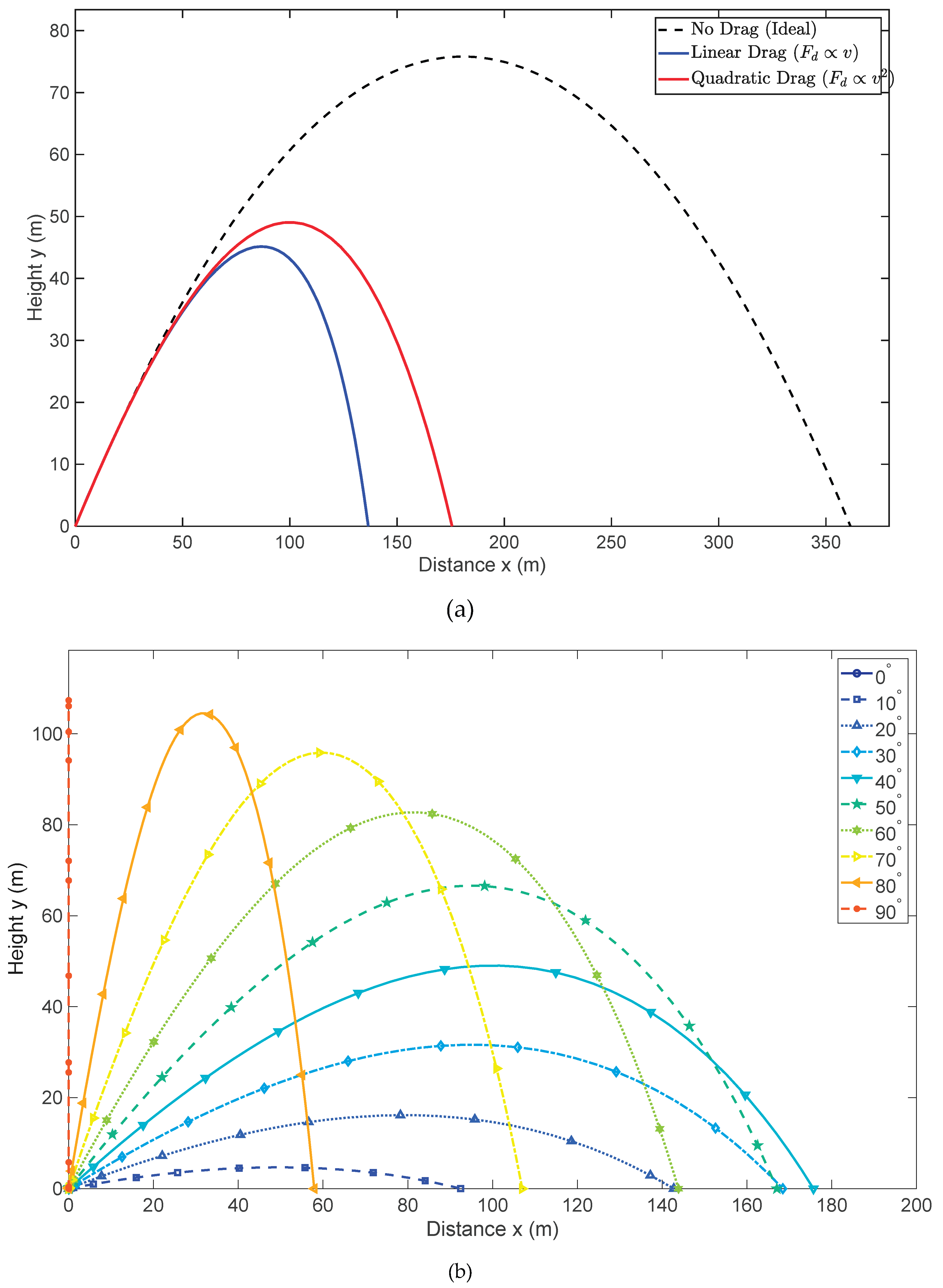
Figure 2.
Schematic of the projectile trajectory in the (x, y) Cartesian plane, illustrating the trajectory angle q relative to the horizontal, the arc length path coordinate l, and the velocity vector components resolved in intrinsic coordinates (tangential vta and normal vn).
Figure 2.
Schematic of the projectile trajectory in the (x, y) Cartesian plane, illustrating the trajectory angle q relative to the horizontal, the arc length path coordinate l, and the velocity vector components resolved in intrinsic coordinates (tangential vta and normal vn).
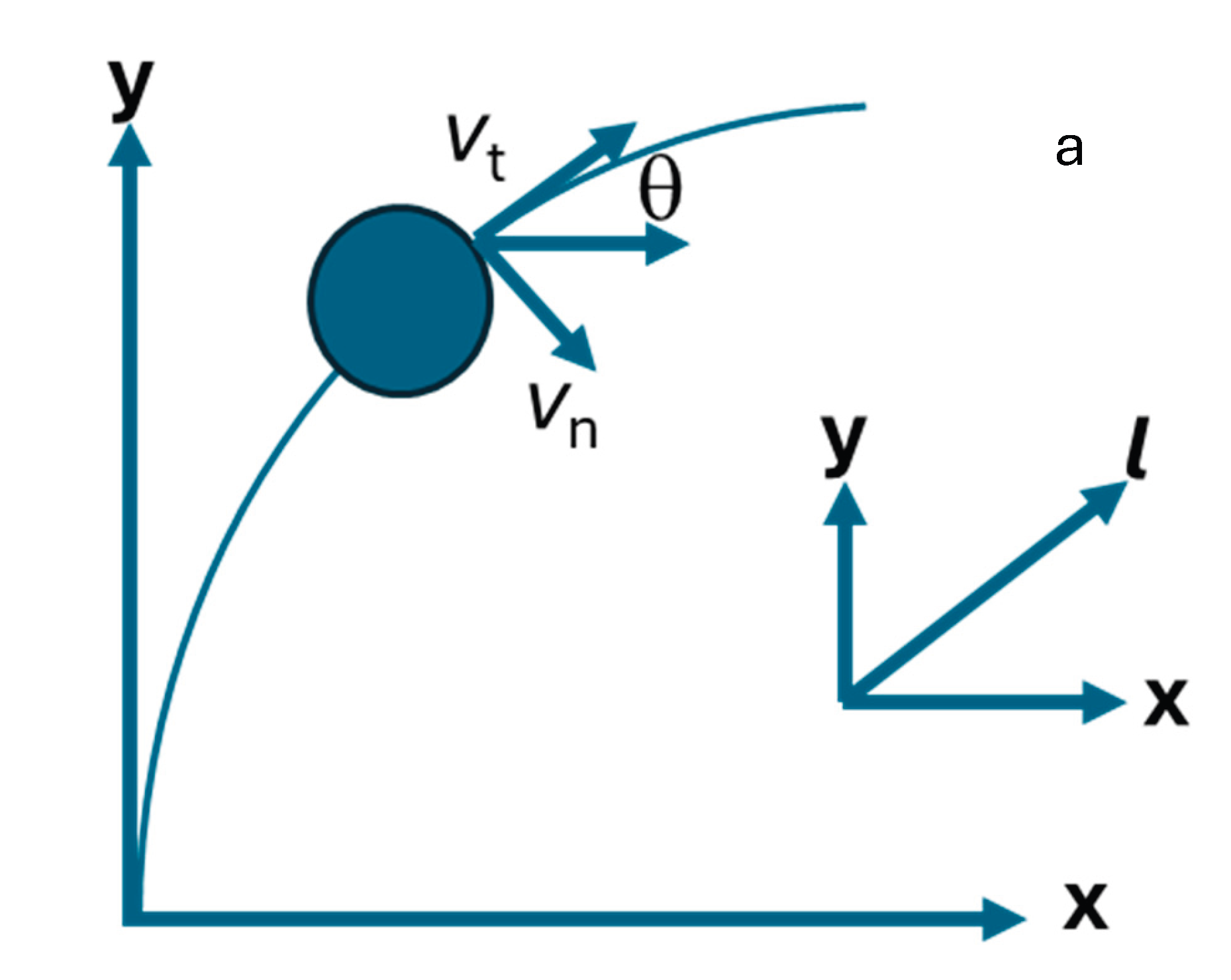
Figure 3.
Velocity evolution in time during the path of the ball until reaching the terminal velocity.
Figure 3.
Velocity evolution in time during the path of the ball until reaching the terminal velocity.
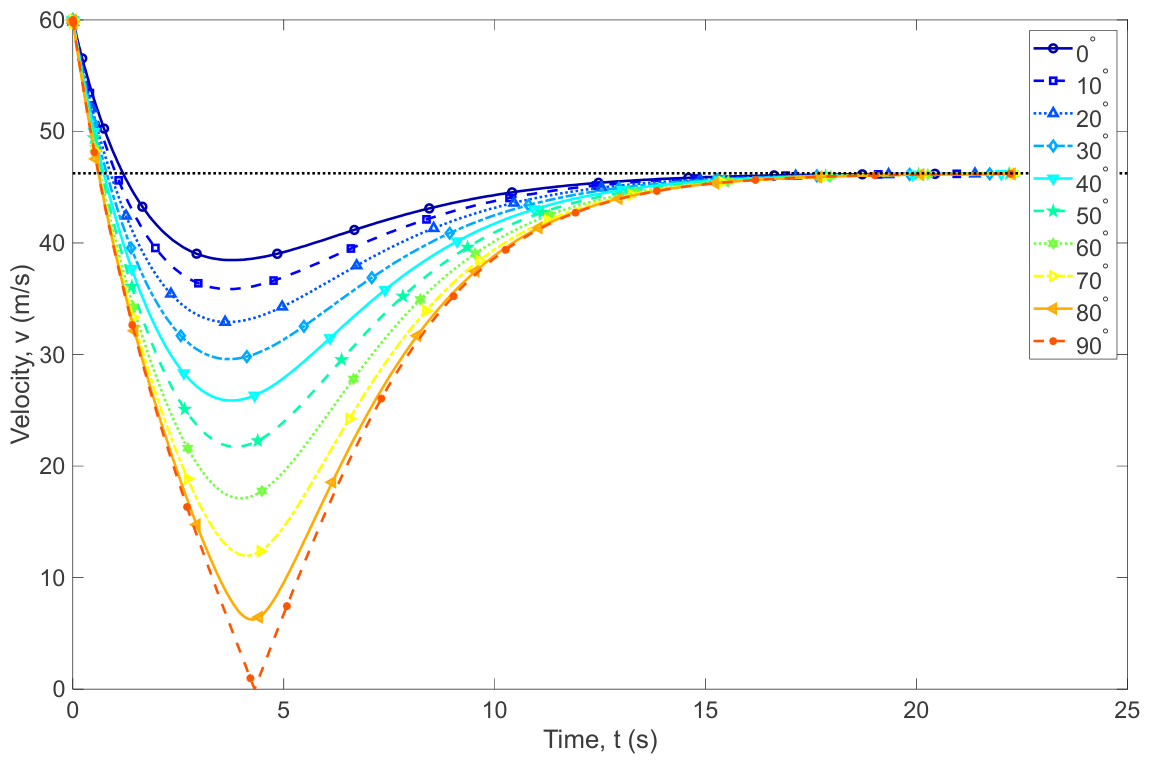
Figure 4.
a) . Thermodynamic entropy production as a function of the horizontal distance x for different launch angles until the ball reaches 0.999 vt. b) Lost information as a function of the horizontal distance x for different launch angles until the ball reaches 0.999 vt.
Figure 4.
a) . Thermodynamic entropy production as a function of the horizontal distance x for different launch angles until the ball reaches 0.999 vt. b) Lost information as a function of the horizontal distance x for different launch angles until the ball reaches 0.999 vt.
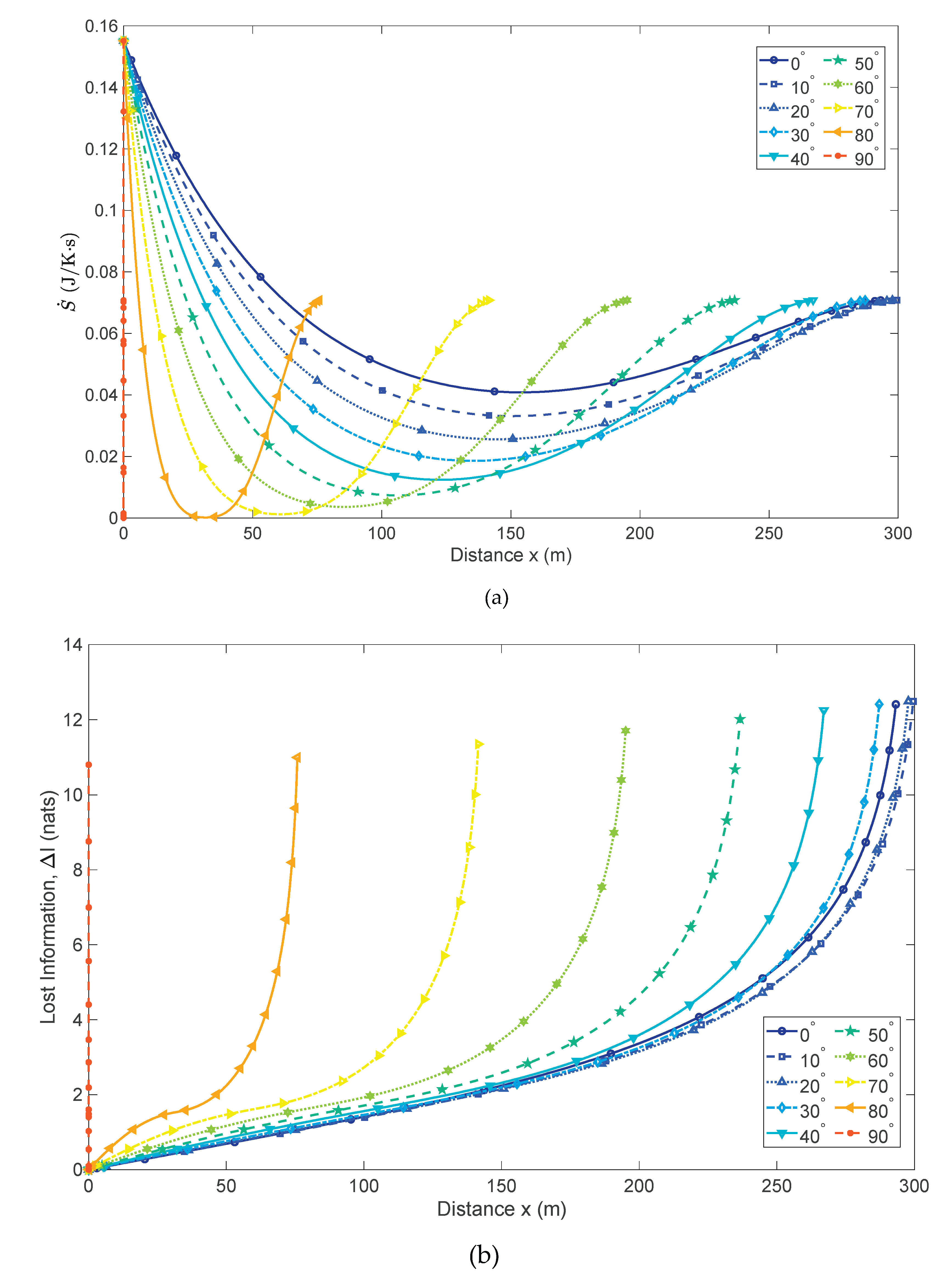
Figure 5.
Evolution of the entropic Lagrange multiplier λ(θ) as a function of the path angle q for different initial launch angles a. As the projectile approaches the vertical asymptote (q -> -90º), the multiplier smoothly converges toward the constant terminal attractor value , illustrating how the dynamic Newtonian constraint balances thermodynamic entropy production near the steady state.
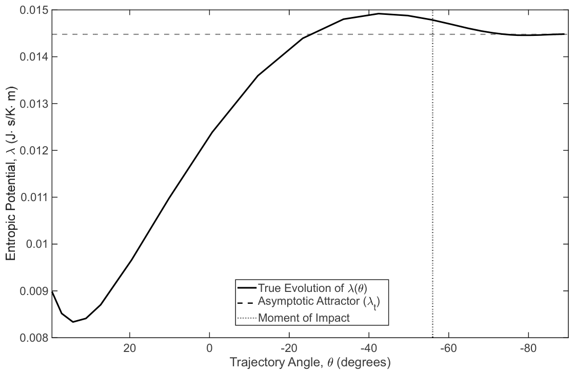
Figure 6.
Entropy production as a function of the angle q for different launch angles until the impact with the ground.
Figure 6.
Entropy production as a function of the angle q for different launch angles until the impact with the ground.
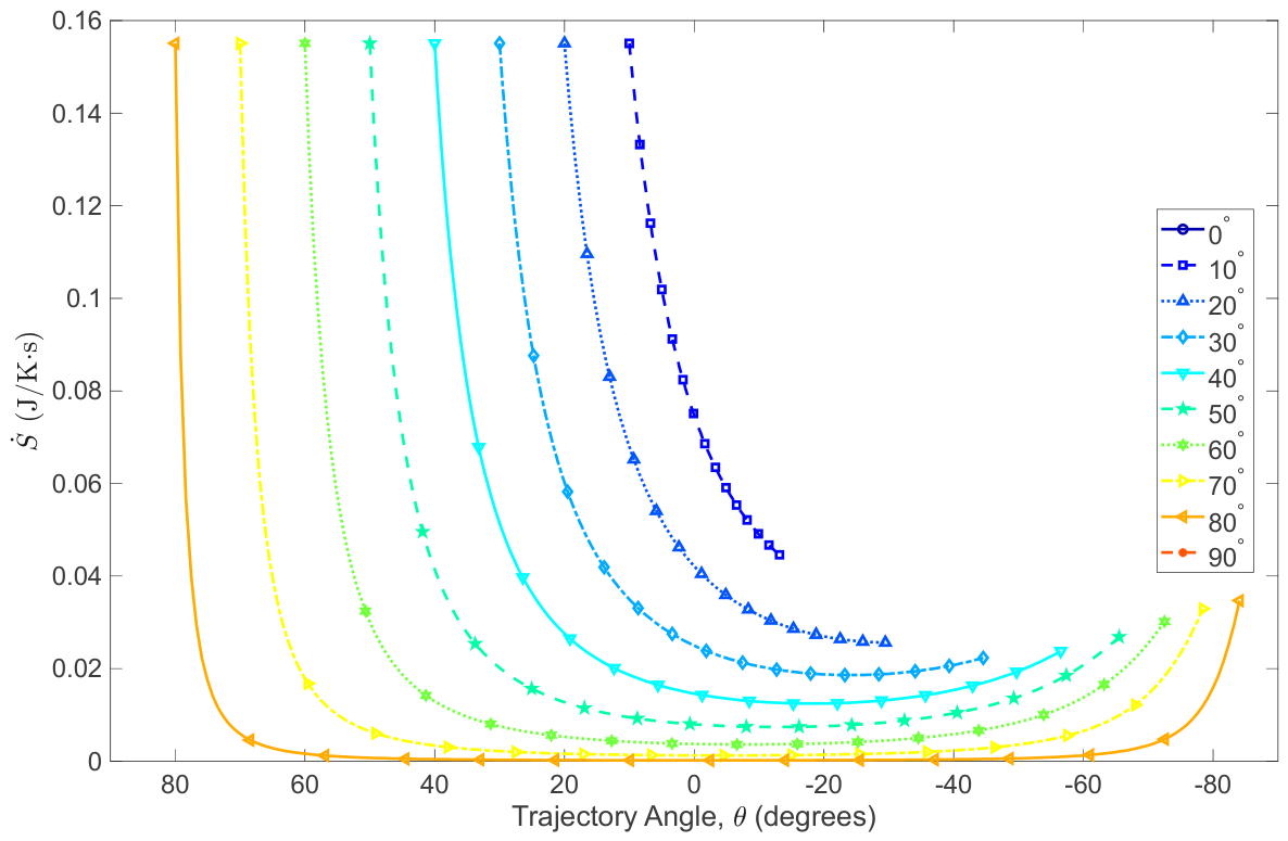
Figure 7.
Maximum x-range as a function of launch angle. The optimal angle is shown with the star on the continuous curve (left axis). In dashed line, the ss straight curve (right axis). The crossing by zero shows the optimal launch angle.
Figure 7.
Maximum x-range as a function of launch angle. The optimal angle is shown with the star on the continuous curve (left axis). In dashed line, the ss straight curve (right axis). The crossing by zero shows the optimal launch angle.
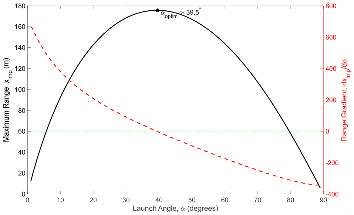
Figure 8.
Comparison of the total entropy generated as a function of the launch angle. Straight line is for total thermodynamic transient until the attractor. Dashed line is constrained to the interval launch-ground impact. Notice that in the first case we have a decreasing curve whereas in the second, we have a curve with a maximum. As the impact range is arbitrarily selected (not fixed by any physical law), no entropy optimisation occurs in this range.
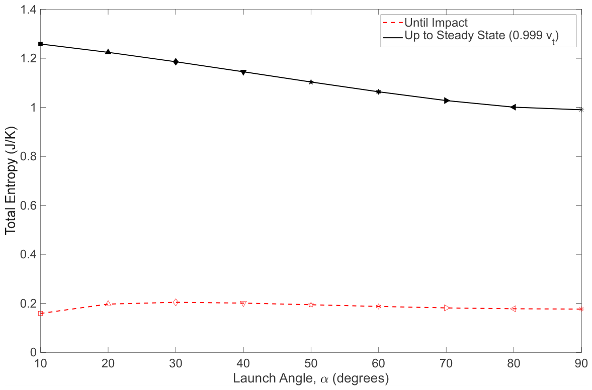
Figure 9.
Duality between macroscopic information loss and thermodynamic entropy generation. Comparison of the total erased kinematic information Hs (in nats, left axis) and the total generated thermal entropy S (in J/K, right axis) as a function of the launch angle a. Although their geometric profiles diverge due to the underlying non-linear relationship (S∝I3), both macroscopic metrics are strictly unified under the dual augmented Lagrangians (, and ,), demonstrating that the continuous phase-space erasure of kinematic information imposes an exact thermodynamic cost.
Disclaimer/Publisher’s Note: The statements, opinions and data contained in all publications are solely those of the individual author(s) and contributor(s) and not of MDPI and/or the editor(s). MDPI and/or the editor(s) disclaim responsibility for any injury to people or property resulting from any ideas, methods, instructions or products referred to in the content. |
© 2026 by the authors. Licensee MDPI, Basel, Switzerland. This article is an open access article distributed under the terms and conditions of the Creative Commons Attribution (CC BY) license (http://creativecommons.org/licenses/by/4.0/).
Copyright: This open access article is published under a Creative Commons CC BY 4.0 license, which permit the free download, distribution, and reuse, provided that the author and preprint are cited in any reuse.