

Submitted:
03 October 2026
Posted:
07 October 2026
You are already at the latest version
Abstract
This paper introduces highFIS, an open-source Python package for training and evaluating high-dimensional Takagi-Sugeno-Kang (TSK) neuro-fuzzy inference systems. TSK systems are widely appreciated for their local linear approximation capabilities and structural transparency, yet the classical product T-norm formulation suffers from exponential rule activation collapse and softmax saturation in high-dimensional spaces. The highFIS library addresses this limitation by unifying thirteen high-dimensional TSK estimator families and a baseline model under a single declarative, scikit-learn-compatible application programming interface (API). These estimators leverage modern mathematical strategies to mitigate the curse of dimensionality, including antecedent exponent re-formulation, differentiable softmin approximations, adaptive parametric T-norms, double groups of gates for sparse feature and rule selection, and head-based subspace decomposition. Every family is implemented with both a Classifier and a Regressor variant that integrate naturally with the meta-estimators and model evaluation frameworks of scikit-learn. Built on PyTorch, the package en-ables efficient gradient-based optimization with hardware acceleration, offers extensive introspection utilities to extract interpretable rule bases, and supports versioned checkpoints for model persistence. Usage is illustrated on a low-dimensional interpretability example and on real high-dimensional classification and regression datasets.
Keywords:
fuzzy systems
; TSK
; neuro-fuzzy
; high-dimensional data
; Python
1. Introduction: High-dimensional TSK fuzzy systems in Python
Takagi-Sugeno-Kang (TSK) fuzzy inference systems [1] are widely used in machine learning because they combine the interpretability of rule-based models with the flexibility of local linear approximation. A TSK system partitions the input space into overlapping fuzzy regions, assigns each region a first-order linear consequent, and produces a prediction as a firing-strength-weighted average of those consequents. Because each rule takes the form of an “if–then” statement with a linear consequent part, TSK systems offer a level of structural transparency that is absent in pure black-box models. Recent high-dimensional TSK variants have been evaluated on gene-expression microarrays, face images, and text-categorization benchmarks with thousands to more than one hundred thousand features [2,3,4], settings in which the ability to inspect individual rules provides value beyond raw predictive accuracy.
Despite this appeal, the classical TSK design carries a well-known weakness in high-dimensional settings. Rule activations are computed as the product of per-feature Gaussian membership degrees, each at most one, so as the input dimension grows this product shrinks exponentially and eventually collapses to zero for every rule simultaneously. The defuzzification denominator then saturates, forcing all rules to contribute equally regardless of the input and stripping the model of its ability to partition the input space effectively. Cui et al. [5] formalized this phenomenon and showed that it is equivalent to the saturation of a softmax function in the log-activation domain. Addressing this curse of dimensionality has since become a central research theme, and several distinct families of architectural strategies have been proposed to mitigate it: (1) antecedent exponent reformulation, which modifies membership functions or normalizations to scale dynamically with the input dimension, as proposed by Cui et al. [5] and Xue et al. [6]; (2) differentiable softmin approximations, which replace the product T-norm with smooth approximations of the minimum operator, as proposed by Xue et al. [7] and Ma et al. [3]; (3) adaptive parametric T-norms, whose parameters are tuned during gradient descent to prevent numerical underflow, as proposed by Xue et al. [2] and Xue et al. [8]; (4) structural gating and regularization, which learn sparse gate functions to suppress irrelevant features and rule pathways, as proposed by Xue et al. [9] and Xue et al. [10]; and (5) subspace decomposition, which projects the high-dimensional input into independent lower-dimensional subspaces to train local rule sets, as proposed by Bian et al. [4].
The Python ecosystem does not yet provide a unified, installable library that covers this landscape. The scikit-fuzzy package [11] provides Mamdani-style inference, fuzzy set operations, and fuzzy clustering, but offers no gradient-trained TSK estimators. The simpful [12] library supports manual construction of both Mamdani and TSK systems with a declarative API, but does not implement data-driven training or any high-dimensional antecedent design. ANFIS-Toolbox [13] provides ANFISRegressor and ANFISClassifier estimators with a scikit-learn-compatible API [14] and supports classic hybrid learning as well as modern gradient-based optimizers; however, it implements Jang’s original product-T-norm architecture [15] and does not include any of the high-dimensional antecedent designs described above. Further Python packages following the same classical design, X-ANFIS [16], ANFISpy [17], lazuardy-anfis [18], and Scikit-ANFIS [19], share this limitation. The closest existing alternative is PyTSK [20], which implements HTSK and LogTSK [5]; it addresses strategy (1) above but does not cover the remaining four strategy families introduced in subsequent literature. Isolated research implementations exist for individual models from those later families, but they are not maintained as installable packages, lack common interfaces, and cannot be combined or compared without substantial reimplementation effort.
Table 1 summarizes this landscape, positioning highFIS against the Python packages discussed above along four axes: coverage of the five high-dimensional strategy families (S1–S5, as introduced above and detailed in Section 3), a scikit-learn-compatible API, a graphics processing unit (GPU)-capable backend, and separate Classifier/Regressor classes.
highFIS fills this gap. It is an open-source Python package, available from the Python Package Index at https://pypi.org/project/highfis and developed at https://github.com/dcruzf/highFIS, that implements thirteen high-dimensional TSK estimator families — together with the classical TSK baseline for reference — under a single scikit-learn-compatible interface, built on the PyTorch automatic differentiation framework [21]. Every estimator family ships both a Classifier and a Regressor variant, and both integrate naturally with meta-estimators and the broader model evaluation framework in scikit-learn. The package also exposes introspection utilities for membership function parameters, rule activation tables, and per-feature importance scores, and provides model serialization. It is designed for practitioners who wish to apply high-dimensional TSK systems without reimplementing models from scratch, and for researchers who need a reproducible reference against which new designs can be benchmarked.
The remainder of this paper is structured as follows. First, Section 2 reviews the mathematical foundations of TSK fuzzy inference systems, formalizes the curse of dimensionality, and details the gradient-based training procedure. Next, Section 3 surveys the high-dimensional estimator families and the classical TSK baseline implemented in highFIS, grouping them by their core dimensionality-reduction strategies. Section 4 then details the software design, package architecture, scikit-learn-compatible API, and introspection utilities of the library. Practical usage is demonstrated in Section 5 through worked examples on real datasets. Finally, Section 6 summarizes the package’s contributions and outlines future development directions.
2. TSK Fuzzy Inference Systems
This section formalizes the standard TSK model, analyzes the saturation phenomenon that motivates high-dimensional models, and describes the gradient-based training procedure shared by all estimator families.
2.1. Standard TSK Model
Let the training dataset be , where is the D-dimensional input feature vector, and is the target output vector. A Takagi-Sugeno-Kang (TSK) fuzzy inference system with R fuzzy rules partitions the input space into overlapping fuzzy regions and assigns a local first-order linear consequent to each region. The r-th fuzzy rule () is defined as:
where is the fuzzy set associated with the d-th feature in the r-th rule, and (for ) represents the consequent parameter vectors. In a regression task, and the rule consequents are scalar values; in a multi-class classification task, C corresponds to the number of classes.
When Gaussian membership functions (MFs) are employed to model the fuzzy sets, the membership degree of the input feature to the fuzzy set is computed as:
where and represent the center and the spread (standard deviation) of the Gaussian function, respectively.
To aggregate the membership degrees across all input dimensions and calculate the activation level of the rule, a fuzzy T-norm operator is applied. By using the standard product T-norm, the raw firing strength of the r-th rule is given by:
The final output of the TSK fuzzy system is the firing-strength-weighted average of the individual rule consequents:
where is the normalized firing level of Rule r:
2.2. The Saturation Phenomenon
The normalization of the rule firing levels can be equivalently interpreted in the log-activation domain. Let represent the log-firing strength of Rule r:
Substituting Equation 6 into Equation 5 yields:
which is mathematically identical to the standard softmax function applied to the vector of log-firing strengths .
As the input dimensionality D increases, the log-firing strengths accumulate non-positive terms over all D features. Consequently, when the spreads are initialized independently of D (e.g., around a fixed value like 1), the log-firing strengths decrease rapidly towards . This leads to two critical challenges:
- 1.
- Numerical underflow: The raw firing strengths eventually fall below the smallest representable floating-point value (approximately in double precision, and in single precision), collapsing to exactly zero for all rules. In this case, the denominator in Equation 5 becomes zero and the normalized firing levels evaluate to , so the output and every gradient become not-a-number (NaN) values. To prevent absolute numerical underflow, the common softmax stabilization trick is used:where .
- 2.
- Softmax saturation: Although Equation 8 prevents division-by-zero, it does not resolve the curse of dimensionality. Because each is a sum of D non-positive terms, any systematic difference in how well two rules match the input accumulates over the features, so the absolute differences typically grow proportionally to D. As a result, the stabilized softmax function saturates: the rule that happens to be closest to the input vector (having the maximum ) receives a normalized firing strength of approximately 1, while all other rules receive firing strengths of approximately 0:
When softmax saturation occurs, the TSK model loses its capacity for fuzzy partitioning. The system behaves like a hard nearest-prototype classifier or a single nearest-neighbor model. Crucially, the derivatives of the softmax function with respect to the input or antecedent parameters approach zero for all non-fired rules. This vanishing gradient problem prevents the antecedent parameters of inactive rules from learning from data, leaving the system in a state where only a single rule is updated. The resulting loss landscape is flat over most of the parameter space, causing gradient-based training to stall or oscillate, and severely degrading generalization performance [5].
Both challenges concern numerical range, not precision: at a raw firing strength of order underflows in 64-bit arithmetic exactly as in 32-bit, and the growth of with D is a property of the sums in Equation 6, not of how they are stored. The strategies of Section 3 therefore reformulate the computation rather than widen the number format, which is why the results reported here are computed in single precision.
2.3. Gradient-Based Optimization
To optimize the TSK fuzzy system, all parameters — including antecedent centers , spreads , and consequent parameters — are trained simultaneously using gradient-based optimization. Assuming a dataset of N training samples, the classical formulation minimizes the mean squared error (MSE) loss function:
where is the c-th component of the system output on the n-th sample, and is the corresponding target value. In highFIS, every regressor uses this loss, and so do the classifiers of the high-dimensional families, applied to one-hot encoded targets as in their source articles. The TSKClassifier, HTSKClassifier, and LogTSKClassifier estimators, whose source articles prescribe no classification loss, use the cross-entropy loss on the softmax of the outputs instead.
The gradients of this loss with respect to the centers, spreads, and consequent coefficients are obtained by automatic differentiation, and the parameters are updated iteratively by mini-batch gradient descent, for any parameter , with learning rate . Every antecedent gradient carries the factor , which is why the saturation of Section 2.2 starves all but the winning rule of updates. In highFIS, each family uses the optimizer of its source article: plain stochastic gradient descent (SGD) for AdaTSK, FSRE-ADATSK, and DG-TSK; Adam [22] for ADPTSK, DombiTSK, ADMTSK, AYATSK, and DG-ALETSK; and AdamW [23] for the classical baseline, HTSK, LogTSK, HDFIS, and MHTSK, all as implemented in PyTorch [21].
3. High-Dimensional TSK Estimators
To address the numerical underflow and softmax saturation challenges detailed in Section 2.2, several high-dimensional TSK fuzzy system architectures have been proposed in the literature. These methods, all implemented in the highFIS package, can be classified into five primary mathematical strategies: antecedent exponent reformulation, differentiable softmin approximations, adaptive parametric T-norms, structural gating and regularization, and subspace decomposition.
Crucially, as explored below, several of these models are hybrid systems that combine features from multiple strategies (e.g., merging structural gating regularization with softmin T-norm approximations) to maximize both stability and sparsity in high-dimensional spaces.
Table 2 summarizes the classical baseline and the thirteen high-dimensional estimator families implemented in highFIS, grouped by strategy, together with their estimator classes and source references.
Several of the families below rely on the constants 690, 700, or 745 (Equations 13 and 15, and the adaptive ln-exp (ALE) softmin of Section 3.4). They derive from the exponent range of IEEE 754 double precision, whose largest finite value has logarithm and whose smallest subnormal has logarithm : AdaTSK’s 690 and DG-ALETSK’s keep terms such as below the overflow boundary, while HDFIS-prod’s targets the underflow boundary so that no firing strength becomes exactly zero. highFIS preserves the exact constant of each source article. The softmin constants are also safe in single precision, whose range is far narrower (), because the Ada-, ADP-, and ALE-softmin operators are evaluated in log-sum-exp form and never exponentiate them directly. HDFIS-prod is the exception: its bound holds only in double precision, which highFIS uses when PyTorch’s default floating-point type is set to torch.float64.
3.1. Antecedent Exponent Reformulation
This strategy targets the Gaussian exponent directly, either by scaling it at the antecedent level to prevent underflow, or by modifying the normalization step to avoid exponentiation entirely.
-
High-dimensional TSK (HTSK): Developed by Cui et al. [5] and implemented via the classes HTSKClassifier and HTSKRegressor, this model replaces the standard sum in the log-firing strength exponent (Equation 6) with an average:Mathematically, this is equivalent to scaling the Gaussian spreads by a factor of . By forcing the exponent to scale inversely with D, the individual membership degrees are kept close to 1, preventing the firing strengths from decaying exponentially to zero.
-
Log-space TSK (LogTSK): Also analyzed by Cui et al. [5] and implemented via LogTSKClassifier and LogTSKRegressor, this model avoids the softmax saturation of Equation 9 by modifying the normalization step. Instead of exponentiating the log-firing strengths , LogTSK performs defuzzification using a log-transformed formulation where the normalized firing strength is computed directly in log-space:Because Equation 12 uses normalization over the reciprocal log-firing strengths rather than a softmax over exponential firing strengths, it is immune to computer precision underflow and yields sparser, more interpretable rule activations.
-
High-dimensional fuzzy inference system (HDFIS): Proposed by Xue et al. [6], this family implements two complementary approaches to handle high-dimensional tasks:
- HDFIS-prod (HDFISProdClassifier and HDFISProdRegressor) resolves the product T-norm underflow of Equation 3 while preserving rule specificity. Based on the computer’s floating-point precision limit (where the underflow limit is defined by with ), they derive a lower bound for the membership spreads:where the scaling exponent is dynamically bounded by . This ensures that , keeping the membership functions as narrow (specific) as possible.
-
HDFIS-min (HDFISMinClassifier and HDFISMinRegressor) replaces the product T-norm with the minimum T-norm:Because the minimum operator is non-differentiable, HDFIS-min sidesteps the vanishing gradient issue by keeping the antecedent parameters fixed at their initial values and optimizing only the consequent parameters via gradient descent or least squares estimation (LSE).
3.2. Differentiable Softmin Approximations
Rather than using the product T-norm, which accumulates dimensionality across all D features, this family of models employs approximations of the minimum T-norm. Since the minimum T-norm only depends on the feature with the worst membership value, it is inherently immune to the curse of dimensionality. However, because the minimum operator is non-differentiable, it must be approximated by a differentiable softmin function.
- Adaptive TSK (AdaTSK): Introduced by Xue et al. [7] and implemented via ADATSKClassifier and ADATSKRegressor, this model computes the firing strength using an adaptive softmin (Ada-softmin) operator:where the parameter is updated adaptively at each sample based on the minimum membership value:with clamped between and . This prevents the terms from exceeding the maximum representable double-precision float (), avoiding numerical overflow while providing a tight approximation to the minimum operator.
- Adaptive double-parameter softmin TSK (ADPTSK): Developed by Ma et al. [3] and implemented via ADPTSKClassifier and ADPTSKRegressor, this model addresses the limitation that AdaTSK can still crash if the membership function outputs a value of absolute zero (which makes the logarithm undefined). To prevent this, they introduce a Gaussian membership function with a positive infimum (Gaussian PIMF):where is a user-defined parameter, ensuring the membership degree is strictly bounded below by . They couple this with the ADP-softmin operator, which uses two adaptive parameters, q and , to approximate the minimum T-norm even more closely without numerical failure:where q and are jointly computed from the minimum and maximum membership values in Rule r.
3.3. Adaptive Parametric T-Norms
This strategy uses classic parametric T-norms from fuzzy logic theory and sets their parameter adaptively from the input dimension, so that the aggregated firing strength stays away from zero and numerical underflow is prevented.
-
Dombi-based TSK (DombiTSK and ADMTSK): Proposed by Xue et al. [2], this family implements two approaches:
- DombiTSK (DombiTSKClassifier and DombiTSKRegressor) leverages a fixed Dombi parameter for the Dombi T-norm.
- ADMTSK (ADMTSKClassifier and ADMTSKRegressor) computes firing strengths using an adaptive Dombi T-norm:where the Dombi parameter is not tuned by hand but set from the input dimension,with the positive lower bound of the membership functions and a heuristic constant (the k argument). The parameter is computed once, when the model is built, and is shared by all rules; it grows with D, so the T-norm moves toward the minimum T-norm as the dimension increases and the firing strengths do not vanish with D.
- Adaptive Yager TSK (AYATSK): Developed by Xue et al. [8] and implemented via AYATSKClassifier and AYATSKRegressor, this model leverages the Yager T-norm:where the Yager parameter is set from the input dimension and the lower bound of the membership functions as . With this choice the sum cannot exceed , so the clipping at zero in Equation 21 is never triggered and the rule activation does not collapse as D grows. As in ADMTSK, is computed once when the model is built and is shared by all rules.
3.4. Structural Gating and Regularization
Rather than altering T-norms directly, this strategy embeds trainable gate functions into the system to perform feature selection and rule pruning, removing irrelevant inputs to lower the effective dimensionality. Several hybrid systems combine gating with softmin operators.
- Double groups of gates TSK (DG-TSK): Developed by Xue et al. [9] and implemented via DGTSKClassifier and DGTSKRegressor, this model incorporates antecedent feature gating:where is a gate function. When the gate value approaches 0, the membership value becomes 1, bypassing the feature d in the T-norm calculation. Consequent gates are also applied to prune redundant rules. Regularization on the gate parameters drives them to be sparse, performing feature selection and rule extraction simultaneously during optimization.
- Double-gate adaptive ln-exp TSK (DG-ALETSK): Proposed by Xue et al. [10] and implemented via DGALETSKClassifier and DGALETSKRegressor, this is a hybrid model that combines the double groups of gates (DG) structure with the adaptive ln-exp softmin (ALE-softmin) operator:where (with ). This combination allows the model to perform sparse feature selection while benefiting from the dimensionality-invariance of the softmin T-norm.
- FSRE-ADATSK: Proposed by Xue et al. [7] and implemented via the FSREADATSKClassifier and FSREADATSKRegressor classes, this is a hybrid model combining the sequential feature selection and rule extraction (FSRE) gate protocols with the Ada-softmin T-norm approximation. It is trained in a three-phase procedure: (1) feature selection using antecedent gates, (2) rule extraction using consequent gates, and (3) fine-tuning of the remaining parameters.
3.5. Subspace Decomposition Strategy
- Multihead TSK (MHTSK): Developed by Bian et al. [4] and implemented via MHTSKClassifier and MHTSKRegressor, this model decomposes the high-dimensional feature space into H lower-dimensional subspaces (heads). Each head computes its own local rule activations and consequents over a small number of features, preventing numerical underflow in the rule layer. The outputs from all heads are then aggregated in a final multihead layer, providing a highly scalable and stable architecture for very large datasets. The number and size of the heads are configurable; by default the library sets them so that the union of the random feature subsets covers a high fraction (about ) of the inputs, which is precisely what allows the decomposition to keep a foothold on the informative features even when they form a small minority of a high-dimensional input.
4. Software Design and Architecture
The highFIS package provides a unified, extensible, and computationally efficient framework for training high-dimensional TSK fuzzy inference systems in Python. Its design bridges two popular ecosystems: the user-facing interface adheres strictly to the API design principles of scikit-learn [14], while the computational backend leverages PyTorch [21] for gradient-based optimization and hardware acceleration.
4.1. Separation of concerns: estimators versus PyTorch models
To ensure modularity and maintainability, the library decouples the high-level user interface from the underlying computational graph. This is achieved via a two-tier package structure:
- highfis.estimators:
- This subpackage exposes the estimator classes (e.g., HTSKClassifier, DGALETSKRegressor) that are instantiated and manipulated by the end-user. These classes inherit from the abstract base classes _BaseClassifierEstimator and _BaseRegressorEstimator, which extend scikit-learn’s BaseEstimator together with its ClassifierMixin and RegressorMixin, respectively. They manage input data validation, hyperparameter handling, training orchestration, and model serialization. Through this inheritance every estimator is a drop-in scikit-learn predictor, composing without adaptation with the hyperparameter searchers (GridSearchCV(), RandomizedSearchCV(), and the halving variants), the cross-validation utilities (cross_val_score(), cross_validate(), cross_val_predict()), Pipeline(), and ensemble meta-estimators such as bagging, voting, stacking, and (for the classifiers) probability calibration. Section 5.1 exercises GridSearchCV() directly.
- highfis.models:
- This subpackage defines the actual neuro-fuzzy network architectures as subclassed torch.nn.Module instances. When an estimator is fitted, it instantiates its corresponding PyTorch model, transferring training tensors to the designated execution device: the central processing unit (CPU), an NVIDIA GPU via CUDA, or Apple Silicon via Metal Performance Shaders (MPS).
4.2. Package Structure and Component Inventory
The highFIS library is structured into several self-contained modules, each responsible for a specific aspect of the neuro-fuzzy pipeline. A complete inventory of the key modules and their components includes:
- highfis.memberships:
-
Exposes a library of 19 differentiable membership function classes. This includes classical Gaussian (GaussianMF) with learnable center m and spread , and piecewise polynomial shapes (e.g., TriangularMF, TrapezoidalMF, PiMF). Additionally, it features advanced formulations designed for high-dimensional stability:
- ConstantMF: Returns a membership degree of regardless of the input value. This models a “don’t care” condition, enabling sparse rules where only a subset of features are active.
- DimensionDependentGaussianMF: Scales spreads dynamically using the input dimension D, computing to prevent exponential firing strength collapse.
- GaussianPiMF: Implements the Gaussian membership function with a positive infimum used by ADPTSK (Equation 17); its output never falls below , with , which keeps the logarithms of the softmin operators finite.
- highfis.t_norms:
- Implements 8 T-norm operators that inherit from a common BaseTNorm class, in four groups: the two classical operators (ProductTNorm and MinimumTNorm); the geometric mean (GMeanTNorm), which averages the log-memberships over the D features in the spirit of the HTSK reformulation; the Dombi operators, with a fixed parameter (DombiTNorm) or a parameter set from the input dimension as in Equation 20 (AdaptiveDombiTNorm); and the Yager operators (YagerTNorm, YagerSimpleTNorm, which omits the clipping at zero, and ALESoftminYagerTNorm, which replaces that clipping with the ALE-softmin of Section 3.4). The Ada- and ADP-softmin operators of Section 3.2 are implemented as dedicated rule layers rather than as T-norm classes, because their exponent depends on the memberships of each sample and rule.
- highfis.defuzzifiers:
- Implements 4 distinct normalization methods to transform raw firing strengths into probability-like rule weights. Beyond standard sum-based L1 division, it includes log-space softmax normalization (SoftmaxLogDefuzzifier and the temperature-scaled LogSumDefuzzifier) and the scale-invariant inverse-log defuzzifier (InvLogDefuzzifier).
- highfis.optim:
- Houses the training loop managers, providing 3 specialized optimizer classes. While GradientTrainer coordinates standard single-phase mini-batch gradient updates, DGTrainer and FSRETrainer implement complex multi-phase training schedules required for data-guided rule pruning and sequential gate parameter tuning.
- highfis.clustering:
- Integrates clustering wrappers for KMeans, MiniBatchKMeans, and Fuzzy C-Means (FuzzyCMeans) to automate membership function center placement during initialization.
- highfis.persistence:
- Manages file I/O using a versioned schema, enabling fitted models to be saved and loaded safely via save_checkpoint() and load_checkpoint().
4.3. Modular Computation Graph: Layers and Defuzzifiers
Within the PyTorch layer, any TSK model is represented as a feed-forward neural network inheriting from the abstract class BaseTSK (defined in highfis.base). This class organizes the computation into four sequential stages:
- 1.
- Fuzzification layer (highfis.layers.MembershipLayer): Receives the raw input vector and evaluates the membership values according to the feature-wise fuzzy membership functions defined in highfis.memberships.
- 2.
- Rule antecedent layer (highfis.layers.RuleLayer): Aggregates individual membership values into raw rule firing strengths . It accepts a configurable rule base (e.g., Cartesian, compactly combined, or custom indexes) and a T-norm operator from highfis.t_norms.
- 3.
- Normalization defuzzifier (highfis.defuzzifiers): Normalizes the raw firing strengths to obtain rule weights. Each family uses the normalization of its source article: the sum-based L1 division (SumBasedDefuzzifier) for the classical baseline and most families, the log-domain SoftmaxLogDefuzzifier for HTSK and the gated families, and InvLogDefuzzifier for LogTSK; any of them can be passed explicitly. The sum-based and softmax normalizers floor the firing strengths at the machine epsilon of the working precision, so a rule base whose strengths all underflow yields equal weights rather than NaN values.
- 4.
- Consequent layer: Combines the normalized rule weights with local linear functions of the input to yield the final system output.
By structuring the pipeline into distinct PyTorch modules, developers can easily extend the library. For example, adding a new T-norm or a novel membership function family merely requires implementing a new module or class complying with the corresponding base interfaces, leaving the rest of the training and optimization logic untouched.
4.4. Configuring the Fuzzy System
Beyond the choice of estimator family, users shape the fitted system through a small set of declarative constructor arguments, summarized in Table 3. The paragraphs below group the structurally important ones along three axes: how the fuzzy sets are initialized, how they are combined into a rule base, and how the parameters are optimized.
4.4.0.1. Membership function initialization.
The mf_init argument selects how membership centers are placed before gradient tuning:
- Grid ("grid"):
- Places membership centers uniformly across each feature’s range. It is suitable for low-dimensional systems but, combined with a Cartesian rule base, causes exponential rule growth ( rules).
- Clustering ("kmeans", "fcm", or a clusterer):
- Uses k-means or fuzzy c-means clustering — or any user-supplied KMeans, MiniBatchKMeans, or FuzzyCMeans instance — to map rule centers directly to data-driven prototypes, with spreads initialized from cluster-wise variances. This is the default ("kmeans").
- Point-based (rule_base = "pfrb"):
- Sets membership centers to the feature values of a selected subset of training samples, with spreads proportional to global feature standard deviations, so rules sit exactly where real data points reside.
The companion sigma_scale argument scales the initialized spreads; setting sigma_scale = "auto" multiplies them by , a dimension-aware widening that counteracts firing-strength collapse as D grows.
4.4.0.2. Rule base construction.
The rule_base argument determines how the per-feature fuzzy sets are combined into rules, and its default is resolved from the initialization mode. A Cartesian rule base ("cartesian", the default under grid initialization) enumerates every combination of sets, yielding rules and quickly becoming intractable in high dimensions. The compact-combination base ("coco", the default under clustering initialization) instead binds the r-th set of every feature into a single rule, so the rule count grows linearly (R rules) rather than exponentially — the structural choice that makes high-dimensional TSK models tractable. The point-based base ("pfrb") likewise yields a linear, data-anchored rule set.
4.4.0.3. Optimization and regularization.
Training minimizes the task loss with the PyTorch optimizer of the family’s source article (SGD, Adam, or AdamW; Section 2.3) over epochs passes at the given learning_rate, with early stopping governed by patience and restore_best. To preserve fuzzy interpretability, highFIS splits the parameters into separate groups: antecedent parameters (membership centers and spreads) are optimized without weight decay, while the weight_decay L2 penalty is applied only to the consequent linear coefficients, encouraging smooth local models without distorting the fuzzy sets. All computation runs on the backend selected by device ("cpu", "cuda", or "mps"). Estimators also accept a per-feature input_configs list, assigning a different number of fuzzy sets to individual inputs when domain knowledge warrants it.
4.5. Introspection, Interpretability, and Persistence
Fuzzy rule-based models are often motivated by their potential for interpretability: unlike a purely black-box predictor, a fitted TSK system exposes membership functions, an explicit rule structure, and local linear consequents that can, in principle, be read and reasoned about. This interpretability is not automatic, however — a high-dimensional model may carry thousands of membership-function parameters — so highFIS makes no claim that its fitted models are effortless to read. What the package provides instead are dedicated utilities that make the learned structure explicit and available for inspection, leaving the interpretation itself to the analyst:
- BaseTSK.get_mf_params(): Returns a serializable dictionary containing the mathematical parameters (e.g., mean and standard deviation) of all membership functions.
- BaseTSK.get_rule_table(): Formulates the rule base as a table showing the mappings between features and fuzzy sets for each rule.
- BaseTSK.get_consequent_weights(): Extracts the linear coefficients of the consequent equations, allowing direct analysis of local model behavior.
These utilities are exercised on a concrete low-dimensional example in Section 5.1, where the fitted fuzzy sets are also plotted; Section 5.2 then discusses why the same inspection becomes far harder to digest at .
For model persistence, highFIS implements a versioned checkpointing mechanism in highfis.persistence. Each estimator exposes an ergonomic save() method and a load() class method (wrapping the lower-level save_checkpoint()/load_checkpoint() functions) that, using PyTorch’s native serialization, store the complete estimator configuration, fitted model weights (state_dict), and scikit-learn metadata. Checkpoints are safeguarded by format version validations to ensure backward compatibility and prevent corrupt state restoration.
4.6. Testing and Quality Assurance
The package is accompanied by a pytest suite of 1029 tests (version 0.29.0) organized by module and by estimator family, which exercises every module and reaches full statement and branch coverage; the build fails if coverage drops below 90%. The suite runs under continuous integration for Python 3.11 to 3.14 on every pull request, and on Linux, macOS, and Windows for every pull request into the release branch. Beyond unit tests of the membership functions, T-norms, defuzzifiers, layers, trainers, and persistence, cross-family guards pin down properties that are easy to break silently: every estimator’s constructor arguments must round-trip through get_params() and clone(), as scikit-learn requires; every model’s default loss must match the one prescribed by its source article (Section 2.3); and each family’s batch_size = "auto" policy must reproduce its article’s protocol. Further family-specific tests check details taken from the source articles, such as the gated bias term of DG-ALETSK and the parameter formulas of the adaptive T-norms. The suite does not attempt to reproduce the numerical results reported in those articles, which depend on preprocessing and tuning protocols that are not always fully specified.
5. Illustrations
This section walks through three illustrations, all reproduced by the standalone replication script jss_replication.py in about half an hour on a free Google Colab CPU runtime. The first, on Fisher’s Iris data, exercises the inspection tools of Section 4.5, scikit-learn’s GridSearchCV(), and model persistence. The second and third compare the classical baseline with one representative family per mitigation strategy of Table 2 on two genuinely high-dimensional problems: classification on the Colon microarray data () and regression on the Tecator spectra ().
These are illustrations of how the software is used, not a controlled comparison of the estimator families. A single 80/20 split, five-fold cross-validation inside the training part, hyperparameters chosen per family, and no statistical testing suffice to show that each family trains, predicts sensibly, and is inspectable through one API; they do not establish that any family is better than another, and the numbers below should not be read as a ranking.
5.1. Model Inspection, Interpretability, and Integration
The first example is deliberately pedagogical: a small dataset on which every part of a fitted model can be printed and plotted. We use Fisher’s Iris data ( features, three species), normalized to and split 80/20. We fix three membership functions per feature, so the compact rule base yields exactly three rules, and let GridSearchCV() select the learning rate and epoch budget under five-fold cross-validation. Two light regularizers are used: weight decay on the linear consequents and a uniform regularization (UR) term [24], weighted by ur_weight, which penalizes the squared deviation of each rule’s average normalized firing strength from and so discourages unused rules. Because every estimator subclasses scikit-learn’s BaseEstimator, the model-selection machinery applies without adaptation:
>>> from sklearn.datasets import load_iris
>>> from sklearn.preprocessing import MinMaxScaler
>>> from sklearn.model_selection import train_test_split, GridSearchCV
>>> from highfis import TSKClassifier
>>> iris = load_iris()
>>> X = MinMaxScaler().fit_transform(iris.data)
>>> X_train, X_test, y_train, y_test = train_test_split(
... X, iris.target, test_size=0.2, random_state=11, stratify=iris.target)
>>> base = TSKClassifier(n_mfs=3, mf_init="grid", rule_base="coco",
... random_state=1, batch_size=32, ur_weight=0.02, weight_decay=0.2)
>>> grid = {"learning_rate": [0.01, 0.05, 0.1], "epochs": [100, 200]}
>>> search = GridSearchCV(base, grid, cv=5).fit(X_train, y_train)
>>> clf = search.best_estimator_
>>> print(search.best_params_, f"CV={search.best_score_:.3f}")
{’epochs’: 100, ’learning_rate’: 0.01} CV=0.950
The selected configuration has a cross-validated accuracy of . We now inspect how the fitted model trained, what fuzzy partition it learned, and how it behaves on the held-out split.
clf.history_ records, per epoch, the main cross-entropy (train_loss), the UR term (train_ur_loss), their weighted sum (train_total_loss), the training accuracy, and the learning rate, plus a validation loss and the restored best_epoch when fit() is given a validation set. Figure 1 plots the loss and the accuracy of the refitted model: the total loss falls from to and the training accuracy passes by epoch 18, plateauing near , well before the 100-epoch budget.
Next the fuzzy partition. The membership parameters are read back with get_mf_params(); for petal length (x3) the three learned Gaussian sets are:
>>> model = clf.model_
>>> for i, mf in enumerate(model.get_mf_params()["x3"]):
... print(f"MF{i}: mean={mf[’mean’]:.3f}, sigma={mf[’sigma’]:.3f}")
MF0: mean=0.010, sigma=0.104
MF1: mean=0.222, sigma=0.203
MF2: mean=1.364, sigma=0.256
Plotting these over the normalized feature range makes the partition visible directly (Figure 2). For petal length the three sets fall into a low/medium/high pattern — MF0 a narrow set at the low end, MF1 at intermediate values, and MF2 toward large petals — and petal width shows a similar structure. The center of MF2 () lies outside the normalized range, so within that set acts as a right shoulder whose membership rises monotonically toward the largest petals; the learned centers are unconstrained, and this is the kind of detail that plotting the sets makes visible. Sepal width instead receives broad, heavily overlapping sets, consistent with it carrying little class signal on this data.
Finally the rule base and the held-out behavior. The rule table maps each rule to the membership-function index it uses for every feature — under the compact rule base each of the three rules draws the same index across features — and get_consequent_weights() returns the local linear consequents as a rule × class × feature tensor:
>>> for rule in model.get_rule_table():
... print(rule)
>>> model.get_consequent_weights().shape
{’rule_id’: 0, ’x1’: 0, ’x2’: 0, ’x3’: 0, ’x4’: 0}
{’rule_id’: 1, ’x1’: 1, ’x2’: 1, ’x3’: 1, ’x4’: 1}
{’rule_id’: 2, ’x1’: 2, ’x2’: 2, ’x3’: 2, ’x4’: 2}
torch.Size([3, 3, 4])
Two complementary views of the same fitted model are placed side by side in Figure 3. Passing the held-out samples through forward_antecedents() and averaging each rule’s normalized firing strength over the samples of each species gives the rule-activation map (left): its near-diagonal structure shows that the three-rule base has specialized one rule per species — rule 0 fires almost exclusively for setosa (), rule 1 for versicolor (), and rule 2 for virginica (). The right panel comes from the prediction side: evaluate() returns a full metric bundle — including the confusion matrix — in one call.
>>> metrics = clf.evaluate(X_test, y_test)
>>> {k: round(metrics[k], 3) for k in ("accuracy", "balanced_accuracy",
... "precision_macro", "recall_macro", "f1_macro")}
>>> metrics["confusion_matrix"]
{’accuracy’: 1.0, ’balanced_accuracy’: 1.0, ’precision_macro’: 1.0,
’recall_macro’: 1.0, ’f1_macro’: 1.0}
array([[10, 0, 0],
[ 0, 10, 0],
[ 0, 0, 10]])
On this held-out split the model labels all thirty samples correctly. That says more about Iris, a small and nearly separable dataset, than about the estimator; the point of the panel is that rule activations, the metric bundle, and the confusion matrix are each one call away from a fitted model.
At this description (three rules, twelve membership functions, and a consequent tensor) can be read directly. The same calls work unchanged on the Colon model of Section 5.2, but no one reads two thousand fuzzy sets by eye: at high D, highFIS makes the structure accessible rather than self-explanatory, and one turns to aggregate views such as per-feature importances or the learned gate sparsity of the gated families of Section 3.4.
Finally, the fitted model serializes to a versioned checkpoint and restores faithfully — the reloaded estimator scores identically to the original:
>>> clf.save("tsk_iris.pt")
>>> reloaded = TSKClassifier.load("tsk_iris.pt")
>>> print(f"{reloaded.score(X_test, y_test):.3f}")
1.000
5.2. A Genuinely High-Dimensional Classification Problem
We now turn to a genuinely high-dimensional real dataset: the Colon microarray dataset [25], which has gene-expression features but only samples (40 tumor, 22 normal tissues) — a high-dimensional, small-sample classification problem, obtained here from OpenML (data id 45087). The dataset ships alongside the replication script as colon.npz:
>>> import numpy as np
>>> from sklearn.model_selection import StratifiedKFold, train_test_split
>>> from sklearn.preprocessing import MinMaxScaler
>>> from highfis import (TSKClassifier, HTSKClassifier, ADPTSKClassifier,
... ADMTSKClassifier, DGALETSKClassifier, MHTSKClassifier)
>>> data = np.load("colon.npz")
>>> X, y = data["X"], data["y"]
>>> X.shape, np.bincount(y)
((62, 2000), array([40, 22]))
We compare the classical TSKClassifier baseline against one representative family from each of the five mitigation strategies of Table 2: HTSK (S1, antecedent exponent reformulation), ADPTSK (S2, differentiable softmin), ADMTSK (S3, adaptive parametric T-norm), DG-ALETSK (S4, structural gating), and MHTSK (S5, subspace decomposition). Using one family per strategy keeps the illustration legible while still exercising every mitigation mechanism through the same uniform interface; the full roster of families is documented in Section 3.
The protocol mirrors the model-selection arc of Section 5.1. The data are split 80/20 into a training and a held-out test set, stratified by class. Every family is scored by five-fold stratified cross-validation within the training split, with the scaler fitted inside each fold so that no validation sample influences the transform. The test set is untouched until a single family has been selected by that cross-validation, and is then used once. Each family carries its own hyperparameters, since a shared budget would favor whichever design happens to suit it. They were chosen on the training split only, by the same five-fold cross-validation: a grid search, distributed as server/hyperparam_search.py and run with an earlier highFIS release, gave the starting values, which were then refined by hand under that cross-validation for the families the search did not cover or whose scores changed with the current release. The replication script fixes the final values, so the reported results do not depend on rerunning the search.
>>> x_tr, x_te, y_tr, y_te = train_test_split(
... X, y, test_size=0.2, random_state=42, stratify=y)
>>> shared = dict(mf_init="kmeans", rule_base="coco", random_state=42)
>>> families = {
... "TSK (baseline)": TSKClassifier(n_mfs=3, learning_rate=0.1,
... epochs=100, batch_size=64, **shared),
... "HTSK": HTSKClassifier(n_mfs=3, learning_rate=0.01, epochs=100,
... batch_size=64, **shared),
... "ADPTSK": ADPTSKClassifier(n_mfs=3, k=1.5, learning_rate=0.01,
... epochs=100, batch_size=64, **shared),
... "ADMTSK": ADMTSKClassifier(n_mfs=3, k=1.5, learning_rate=0.01,
... epochs=100, batch_size=64, **shared),
... "DG-ALETSK": DGALETSKClassifier(n_mfs=3, mf_init="kmeans",
... dg_epochs=100, finetune_epochs=200, learning_rate=0.1,
... pfrb_max_rules=15, batch_size=32, random_state=42),
... "MHTSK": MHTSKClassifier(n_mfs=3, n_heads=5, learning_rate=0.1,
... epochs=200, batch_size=32, random_state=42),
... }
>>> folds = StratifiedKFold(n_splits=5, shuffle=True, random_state=42)
>>> for name, clf in families.items():
... accs = []
... for tr, va in folds.split(x_tr, y_tr):
... scaler = MinMaxScaler().fit(x_tr[tr])
... clf.fit(scaler.transform(x_tr[tr]), y_tr[tr])
... accs.append(clf.score(scaler.transform(x_tr[va]), y_tr[va]))
... print(f"{name}: {np.mean(accs):.3f} +/- {np.std(accs):.3f}")
TSK (baseline): 0.838 +/- 0.078
HTSK: 0.858 +/- 0.101
ADPTSK: 0.878 +/- 0.074
ADMTSK: 0.878 +/- 0.074
DG-ALETSK: 0.778 +/- 0.095
MHTSK: 0.798 +/- 0.140
Every family’s mean (Figure 4, left) lies between and , all above the majority-class rate, so each extracts signal from the data rather than collapsing. The spread across families is small next to the per-fold standard deviations, which reach ; what the run establishes is that all five mitigation mechanisms are trainable, tunable, and scorable through one interface.
One observation is worth recording, because it shows how the underflow of Section 2.2 manifests in practice rather than bearing on any ranking. With mf_init = "kmeans" and the "coco" rule base (Section 4.4), the baseline has only rules, and at the product of two thousand membership degrees underflows to zero for every rule and every sample. The sum-based normalizer then floors all three strengths at the same machine epsilon, so every rule receives weight exactly for every input: the fitted baseline is no longer a fuzzy partition but a single global linear model, the average of the three linear consequents. HTSK, in contrast, keeps input-dependent normalized weights spread over all three rules. Both remain competitive here because a linear decision function over two thousand gene-expression features already separates most tumor and normal samples of this small dataset; the practical point is that the curse of dimensionality can strip a TSK model of its rule structure without a visible loss of accuracy, which is why inspecting the normalized firing strengths (via forward_antecedents()) is worthwhile even when the scores look healthy.
Cross-validation selects ADPTSKClassifier. It is refit on the full training split and scored once on the held-out test set; beyond score(), every estimator exposes an evaluate() method that returns a full bundle of task-appropriate metrics in one call:
>>> scaler = MinMaxScaler().fit(x_tr)
>>> best = families["ADPTSK"]
>>> best.fit(scaler.transform(x_tr), y_tr)
>>> metrics = best.evaluate(scaler.transform(x_te), y_te)
>>> {k: round(metrics[k], 3)
... for k in ("accuracy", "balanced_accuracy", "f1_macro")}
{’accuracy’: 0.923, ’balanced_accuracy’: 0.9, ’f1_macro’: 0.915}
The returned dictionary also carries precision/recall in both macro and micro forms, the confusion matrix, and the class list. The balanced accuracy () confirms the model is not simply riding the majority class.
With , however, the 20% test set holds only 13 samples — too few to fill a readable confusion matrix. Figure 5 therefore summarizes the cross-validated out-of-fold predictions on the training split, where each of the 49 samples is predicted exactly once by a model that never saw it. The left panel is the confusion matrix (accuracy , the errors split four-to-two between the two tissue types); the right panel plots the accompanying decision margin, the predicted probability of the normal class for every sample grouped by its true label, obtained from predict_proba. The two panels are the same predictions seen two ways: the handful of points that cross the threshold in the margin plot are exactly the off-diagonal counts on the left, and the modest overlap between the groups is an honest picture of how separable the two tissue types are at with only 49 training samples.
5.3. A High-Dimensional Regression Problem
The saturation phenomenon of Section 2.2 is not specific to classification, and neither is the package’s coverage: every family ships with a Regressor variant that switches on a single class name. We demonstrate this on the Tecator dataset [25], a near-infrared spectroscopy benchmark of finely chopped meat samples, each described by spectral absorbance channels; the regression target is the sample’s fat content (in percent), which ranges from about to . Relative to Colon this is a complementary high-dimensional regime — moderate D, strongly correlated continuous features, and a smooth target — so it exercises the regressors on a different kind of problem. The dataset ships as tecator.npz; if the file is absent, the replication script fetches it from OpenML instead.
>>> from sklearn.model_selection import KFold
>>> from sklearn.metrics import r2_score
>>> from highfis import (TSKRegressor, HTSKRegressor, ADPTSKRegressor,
... ADMTSKRegressor, DGALETSKRegressor, MHTSKRegressor)
>>> data = np.load("tecator.npz")
>>> X, y = data["X"], data["y"]
>>> X.shape, (round(float(y.min()), 1), round(float(y.max()), 1))
((240, 100), (0.9, 58.5))
The protocol is the one used for Colon, with stratification dropped because the target is continuous: an 80/20 train/test split, five-fold cross-validation within the training split to compare families and to choose each family’s hyperparameters as for Colon, and a single evaluation on the held-out test set for the family that cross-validation selects. Because the target spans two orders of magnitude, we min-max scale it inside each fold for stable training and report on the original scale.
One selected hyperparameter deserves comment. With the default batch_size = "auto", each family follows the batching protocol of its source article, and on training sets as small as these folds (153 samples here, 39 on Colon) those protocols diverge widely: ADPTSK trains full batch below 500 samples, HTSK and the baseline clamp to , ADMTSK and DG-ALETSK use 10% of the samples, and MHTSK uses 64. Rather than inherit that spread, both illustrations pass an explicit mini-batch size to every family, chosen by the same cross-validation as the other hyperparameters; on small datasets the parameter is worth setting deliberately.
>>> x_tr, x_te, y_tr, y_te = train_test_split(
... X, y, test_size=0.2, random_state=42)
>>> shared = dict(n_mfs=5, mf_init="kmeans", rule_base="coco",
... random_state=42)
>>> families = {
... "TSK (baseline)": TSKRegressor(learning_rate=0.01, epochs=200,
... batch_size=32, **shared),
... "HTSK": HTSKRegressor(learning_rate=0.05, epochs=100,
... batch_size=32, **shared),
... "ADPTSK": ADPTSKRegressor(k=1.5, learning_rate=0.1, epochs=200,
... batch_size=32, **shared),
... "ADMTSK": ADMTSKRegressor(k=1.5, learning_rate=0.2, epochs=200,
... batch_size=32, **shared),
... "DG-ALETSK": DGALETSKRegressor(n_mfs=5, mf_init="kmeans",
... dg_epochs=100, finetune_epochs=300, learning_rate=0.2,
... use_lse=False, batch_size=32, random_state=42),
... "MHTSK": MHTSKRegressor(n_mfs=5, head_size=4, n_heads=25,
... epochs=100, learning_rate=0.2, batch_size=64, random_state=42),
... }
>>> folds = KFold(n_splits=5, shuffle=True, random_state=42)
>>> for name, reg in families.items():
... scores = []
... for tr, va in folds.split(x_tr):
... xs = MinMaxScaler().fit(x_tr[tr])
... ys = MinMaxScaler().fit(y_tr[tr].reshape(-1, 1))
... reg.fit(xs.transform(x_tr[tr]),
... ys.transform(y_tr[tr].reshape(-1, 1)).ravel())
... pred = ys.inverse_transform(
... reg.predict(xs.transform(x_tr[va])).reshape(-1, 1)).ravel()
... scores.append(r2_score(y_tr[va], pred))
... print(f"{name}: {np.mean(scores):.3f} +/- {np.std(scores):.3f}")
TSK (baseline): 0.870 +/- 0.015
HTSK: 0.809 +/- 0.074
ADPTSK: 0.871 +/- 0.057
ADMTSK: 0.888 +/- 0.034
DG-ALETSK: 0.854 +/- 0.074
MHTSK: 0.901 +/- 0.015
Four of the six families land between and mean (Figure 4, right), a range narrower than several per-fold standard deviations. HTSKRegressor () and DGALETSKRegressor () sit lower because of one or two weak folds rather than a consistent deficit.
The gating regressor exposes a numerical subtlety worth surfacing on its own terms. With its default closed-form least-squares consequent solve (use_lse = True) DGALETSKRegressor diverges on some folds, because Tecator’s absorbance channels are so strongly collinear that the least-squares system is ill-conditioned; switching to gradient-trained consequents (use_lse = False, as above) restores stable convergence. This is exactly the kind of per-family knob the uniform constructor interface is meant to expose.
Cross-validation selects MHTSKRegressor, refit on the full training split and scored once on the 48 held-out samples, where it reaches . In Figure 6 the predictions track the ideal line across the full 0– range (left), but the residuals (right) are not structureless: the model shrinks toward the mean, over-predicting the lowest fat contents and under-predicting the highest. The effect is mild, but it is exactly what an aggregate hides and a residual plot surfaces.
The same evaluate() method serves the regressors, returning a regression metric bundle. After refitting the selected MHTSKRegressor and both scalers on the full training split, we score it on the held-out test set (scored on the min-max-scaled target it was trained on, so the scale-free metrics carry over directly and the error metrics are in scaled units):
>>> xs = MinMaxScaler().fit(x_tr)
>>> ys = MinMaxScaler().fit(y_tr.reshape(-1, 1))
>>> best = families["MHTSK"]
>>> best.fit(xs.transform(x_tr), ys.transform(y_tr.reshape(-1, 1)).ravel())
>>> metrics = best.evaluate(xs.transform(x_te),
... ys.transform(y_te.reshape(-1, 1)).ravel())
>>> {k: round(metrics[k], 3)
... for k in ("r2", "pearson", "explained_variance", "mae")}
{’r2’: 0.907, ’pearson’: 0.965, ’explained_variance’: 0.907, ’mae’: 0.064}
The full dictionary also reports the root mean squared error, median and maximum absolute errors, mean bias, percentage and logarithmic errors; the mean bias of shows that the errors cancel on average, even though they depend on the fat level as the residual plot shows.
6. Summary and Discussion
The highFIS package addresses a critical gap in the Python scientific software ecosystem by providing a unified, extensible, and scikit-learn-compatible library for training and evaluating high-dimensional Takagi-Sugeno-Kang (TSK) fuzzy inference systems. By consolidating thirteen distinct estimator families under a single declarative interface, it allows practitioners and researchers to easily implement, combine, and compare models that mitigate the curse of dimensionality.
By integrating PyTorch as its computational backend, highFIS decouples high-level model definition from low-level gradient computation and hardware execution. The library automatically supports CPU- and GPU-accelerated training, automated batching, and standard PyTorch optimizers.
Future development of the package will focus on two primary avenues:
- Online and incremental learning: Exposing PyTorch’s mini-batch execution pipeline via a standard partial_fit API to support out-of-core and streaming data training.
- High-performance scaling: Developing distributed training wrappers to scale execution across multi-GPU environments for massive datasets.
Computational Details
The results in this paper were produced on a Google Colab CPU runtime, using Python 3.14.7 [26] with highFIS 0.29.0, torch 2.13.0 [21], scikit-learn 1.9.0 [14], numpy 2.5.1 [27], and matplotlib 3.11.0 [28]; the allocated CPU was an Intel Xeon at 2.20 GHz (AVX2). The standalone script jss_replication.py pins this stack, fixes all pseudo-random number generator seeds, and reproduces every number and figure in the paper, requiring no network access when the shipped datasets are present.
PyTorch does not guarantee bit-identical floating-point results across environments: the CPU’s vector-instruction path, the thread count, and the exact library build all affect the order of floating-point reductions, so the same code can differ in its last digits on different hardware. Classification accuracy on the small folds is quantized and reproduces across machines, whereas the continuous regression may differ by a few thousandths. We therefore suggest reproducing the results on Google Colab, where the same allocated CPU has reproduced every reported value exactly, across two runtime updates (Python 3.14.5 and 3.14.7); we do not guarantee that environment, however, as its runtime may change over time. The library itself supports any hardware backed by PyTorch, including x86 and ARM CPUs, NVIDIA GPUs via CUDA, and Apple Silicon via MPS.
highFIS is free and open-source software distributed under the GNU General Public License version 3 (GPL-3), and is installable from the Python Package Index via pip install highfis. Its source code, documentation, and issue tracker are hosted at https://github.com/dcruzf/highFIS.
Acknowledgments
We thank the Digital Video Applications Research Center (NPE-LAVID) at the Federal University of Paraíba for its institutional and technical support during the development of this work. We are also grateful to our colleagues and collaborators for their insights, feedback, and encouragement throughout.
References
- Takagi, T.; Sugeno, M. Fuzzy Identification of Systems and Its Applications to Modeling and Control. IEEE Trans. Syst. Man. Cybern. 1985, 15, 116–132. [Google Scholar] [CrossRef]
- Xue, G.; Hu, L.; Wang, J.; Ablameyko, S. ADMTSK: A High-Dimensional Takagi–Sugeno–Kang Fuzzy System Based on Adaptive Dombi T-Norm. IEEE Trans. Fuzzy Syst. 2025, 33, 1767–1780. [Google Scholar] [CrossRef]
- Ma, M.; Qian, L.; Zhang, Y.; Fang, Q.; Xue, G. An Adaptive Double-Parameter Softmin Based Takagi-Sugeno-Kang Fuzzy System for High-Dimensional Data. Fuzzy Sets Syst. 2025, 521, 109582. [Google Scholar] [CrossRef]
- Bian, Z.; Chang, Q.; Wang, J.; Pal, N.R. Multihead Takagi–Sugeno–Kang Fuzzy System. IEEE Trans. Fuzzy Syst. 2025, 33, 2561–2573. [Google Scholar] [CrossRef]
- Cui, Y.; Wu, D.; Xu, Y. Curse of Dimensionality for TSK Fuzzy Neural Networks: Explanation and Solutions. In Proceedings of the Proceedings of the 2021 International Joint Conference on Neural Networks (IJCNN), 2021. [Google Scholar] [CrossRef]
- Xue, G.; Wang, J.; Zhang, K.; Pal, N.R. High-Dimensional Fuzzy Inference Systems. IEEE Trans. Syst. Man. Cybern. Syst. 2024, 54, 507–519. [Google Scholar] [CrossRef]
- Xue, G.; Chang, Q.; Wang, J.; Zhang, K.; Pal, N.R. An Adaptive Neuro-Fuzzy System With Integrated Feature Selection and Rule Extraction for High-Dimensional Classification Problems. IEEE Trans. Fuzzy Syst. 2023, 31, 2167–2181. [Google Scholar] [CrossRef]
- Xue, G.; Yang, Y.; Wang, J. Adaptive Yager T-Norm-Based Takagi–Sugeno–Kang Fuzzy Systems. IEEE Trans. Syst. Man. Cybern. Syst. 2025, 55, 9802–9815. [Google Scholar] [CrossRef]
- Xue, G.; Wang, J.; Zhang, B.; Yuan, B.; Dai, C. Double Groups of Gates Based Takagi-Sugeno-Kang (DG-TSK) Fuzzy System for Simultaneous Feature Selection and Rule Extraction. Fuzzy Sets Syst. 2023, 469, 108627. [Google Scholar] [CrossRef]
- Xue, G.; Wang, J.; Yuan, B.; Dai, C. DG-ALETSK: A High-Dimensional Fuzzy Approach With Simultaneous Feature Selection and Rule Extraction. IEEE Trans. Fuzzy Syst. 2023, 31, 3866–3880. [Google Scholar] [CrossRef]
- Warner, J. (Ed.) scikit-fuzzy: Fuzzy Logic Toolbox for Python; Zenodo, 2024. [Google Scholar] [CrossRef]
- Spolaor, S.; Fuchs, C.; Cazzaniga, P.; Kaymak, U.; Besozzi, D.; Nobile, M.S. Simpful: A User-Friendly Python Library for Fuzzy Logic. Int. J. Comput. Intell. Syst. 2020, 13, 1687. [Google Scholar] [CrossRef]
- França, D.; Aschoff, M.; França, T.; Macedo, D.; França, V.; Cabral, L.; Brito, A.; Siebra, C.; Araujo, T. ANFIS-Toolbox: A Python Package for Adaptive Neuro-Fuzzy Inference Systems. J. Open Res. Softw. 2026, 14. [Google Scholar] [CrossRef]
- Pedregosa, F.; Varoquaux, G.; Gramfort, A.; Michel, V.; Thirion, B.; Grisel, O.; Blondel, M.; Prettenhofer, P.; Weiss, R.; Dubourg, V.; et al. Scikit-Learn: Machine Learning in Python. J. Mach. Learn. Res. 2011, 12, 2825–2830. [Google Scholar]
- Jang, J.S.R. ANFIS: Adaptive-Network-Based Fuzzy Inference System. IEEE Trans. Syst. Man. Cybern. 1993, 23, 665–685. [Google Scholar] [CrossRef]
- Nguyen, V.T. X-ANFIS: An Extensible and Cross-Learning ANFIS Framework for Machine Learning Tasks. Figshare. Software available on Figshare at. 2025. [CrossRef]
- Zaia Monteiro, M. ANFISpy: PyTorch Implementation of Adaptive Neuro-Fuzzy Inference Systems. GitHub. Accessed. 2025. (accessed on 2025-10-20).
- LazuardyTech. lazuardy-anfis: Implementation of Adaptive Neuro-Fuzzy Inference System in Python. GitHub. Accessed. 2024. (accessed on 2025-10-20).
- Zhang, D.; Chen, T. Scikit-ANFIS: A Scikit-Learn Compatible Python Implementation for Adaptive Neuro-Fuzzy Inference System. Int. J. Fuzzy Syst. 2024, 26, 2039–2057. [Google Scholar] [CrossRef]
- Cui, Y.; Wu, D.; Jiang, X.; Xu, Y. PyTSK: A Python Toolbox for TSK Fuzzy Systems. arXiv 2206.03310 2022. [Google Scholar] [CrossRef]
- Paszke, A.; Gross, S.; Massa, F.; Lerer, A.; Bradbury, J.; Chanan, G.; Killeen, T.; Lin, Z.; Gimelshein, N.; Antiga, L.; et al. PyTorch: An Imperative Style, High-Performance Deep Learning Library. In Advances in Neural Information Processing Systems; Curran Associates, Inc., 2019; Vol. 32, pp. 8024–8035. [Google Scholar]
- Kingma, D.P.; Ba, J. Adam: A Method for Stochastic Optimization. In Proceedings of the Proceedings of the 3rd International Conference on Learning Representations (ICLR), 2015. [Google Scholar] [CrossRef]
- Loshchilov, I.; Hutter, F. Decoupled Weight Decay Regularization. In Proceedings of the Proceedings of the 7th International Conference on Learning Representations (ICLR), 2019. [Google Scholar] [CrossRef]
- Cui, Y.; Wu, D.; Huang, J. Optimize TSK Fuzzy Systems for Classification Problems: Minibatch Gradient Descent With Uniform Regularization and Batch Normalization. IEEE Trans. Fuzzy Syst. 2020, 28, 3065–3075. [Google Scholar] [CrossRef]
- Vanschoren, J.; van Rijn, J.N.; Bischl, B.; Torgo, L. OpenML: Networked Science in Machine Learning. SIGKDD Explor. 2013, 15, 49–60. [Google Scholar] [CrossRef]
- Python Software Foundation. Python . Lang. Ref. Version 3.14 2025. [Google Scholar] [CrossRef]
- Harris, C.R.; Millman, K.J.; van der Walt, S.J.; Gommers, R.; Virtanen, P.; Cournapeau, D.; Wieser, E.; Taylor, J.; Berg, S.; Smith, N.J.; et al. Array Programming with NumPy. Nature 2020, 583, 357–362. [Google Scholar] [CrossRef] [PubMed]
- Hunter, J.D. Matplotlib: A 2D Graphics Environment. Comput. Sci. Eng. 2007, 9, 90–95. [Google Scholar] [CrossRef]
Figure 1.
Training trajectory of the selected Iris TSKClassifier, read from history_: total training loss (left) and training accuracy (right) per epoch.
Figure 1.
Training trajectory of the selected Iris TSKClassifier, read from history_: total training loss (left) and training accuracy (right) per epoch.
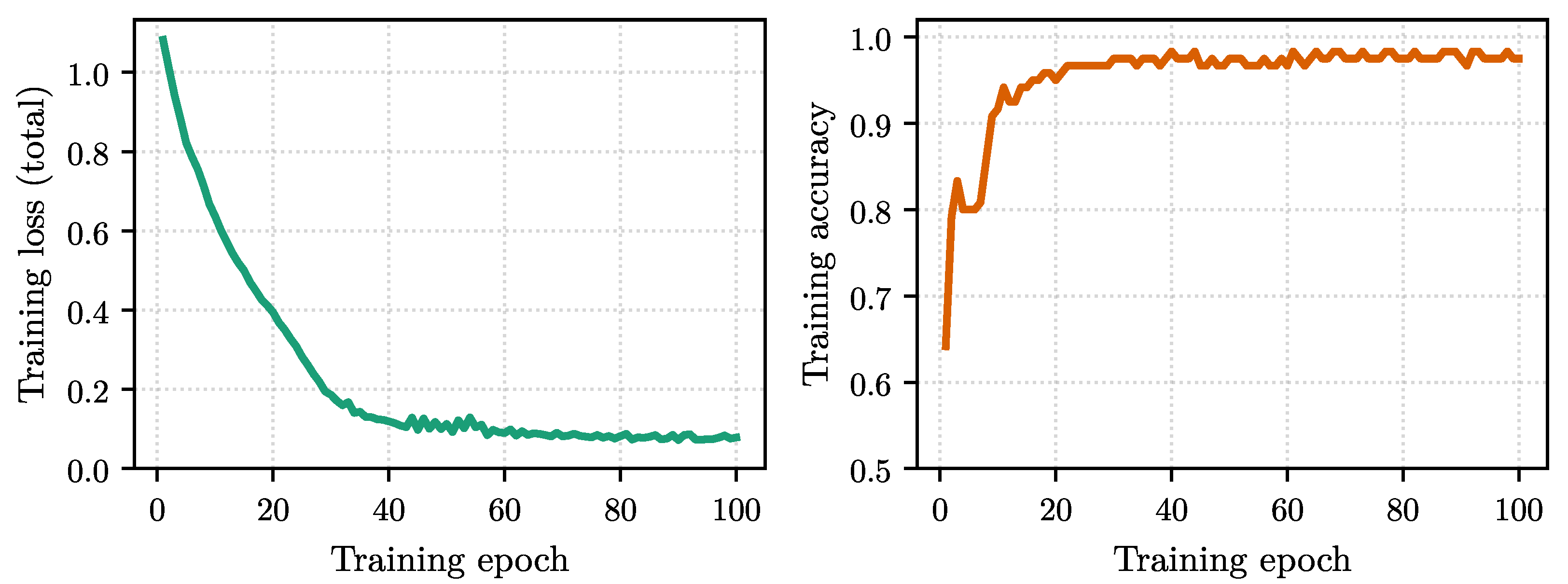
Figure 2.
Trained Gaussian membership functions of the Iris TSKClassifier, one panel per feature, plotted over the normalized feature range. Each curve is one fuzzy set (MF0–MF2), drawn from the parameters returned by get_mf_params().
Figure 2.
Trained Gaussian membership functions of the Iris TSKClassifier, one panel per feature, plotted over the normalized feature range. Each curve is one fuzzy set (MF0–MF2), drawn from the parameters returned by get_mf_params().
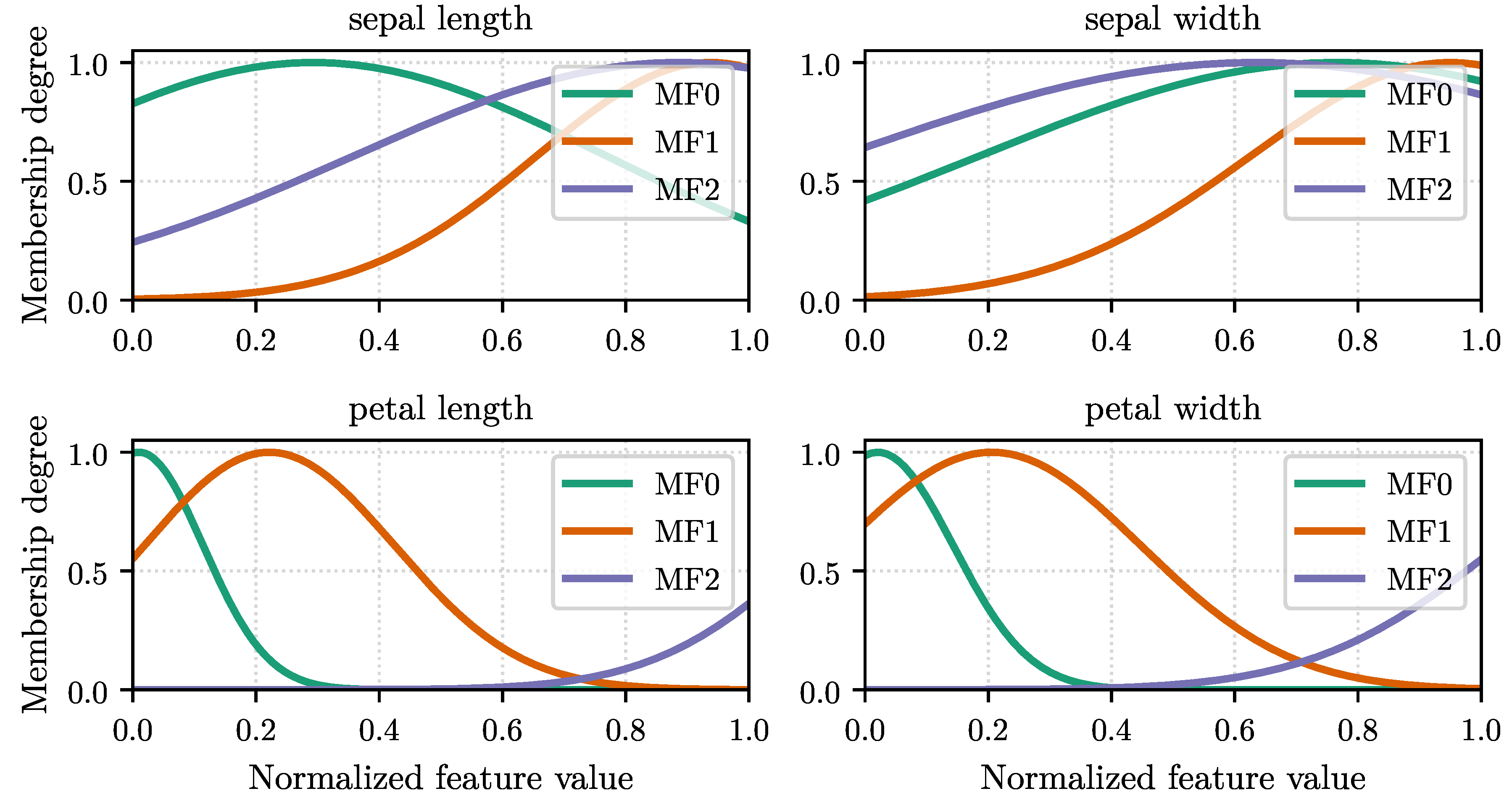
Figure 3.
Two views of the fitted Iris TSKClassifier on the held-out split. Left: mean normalized rule activation per species, from forward_antecedents(). Right: the confusion matrix returned by evaluate().
Figure 3.
Two views of the fitted Iris TSKClassifier on the held-out split. Left: mean normalized rule activation per species, from forward_antecedents(). Right: the confusion matrix returned by evaluate().
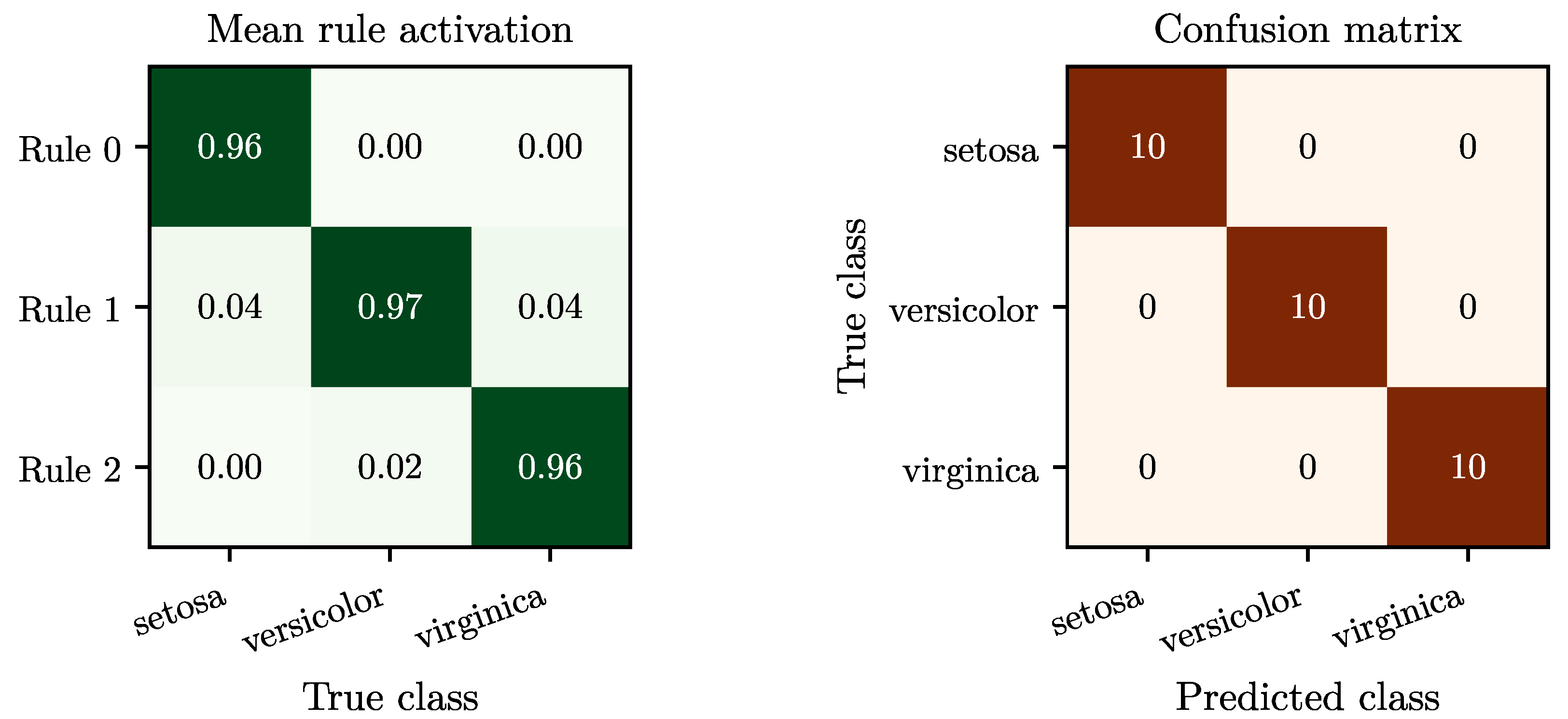
Figure 4.
Cross-validated scores of the classical baseline and five representative families, one per mitigation strategy of Table 2, on the training split of each real dataset. Left: accuracy of the Classifier variants on Colon (, ). Right: of the Regressor variants on Tecator (, ). Each dot is one of the five folds (jittered horizontally) and the black-edged diamond marks the family mean; colors identify the mitigation strategy (baseline in gray).
Figure 4.
Cross-validated scores of the classical baseline and five representative families, one per mitigation strategy of Table 2, on the training split of each real dataset. Left: accuracy of the Classifier variants on Colon (, ). Right: of the Regressor variants on Tecator (, ). Each dot is one of the five folds (jittered horizontally) and the black-edged diamond marks the family mean; colors identify the mitigation strategy (baseline in gray).
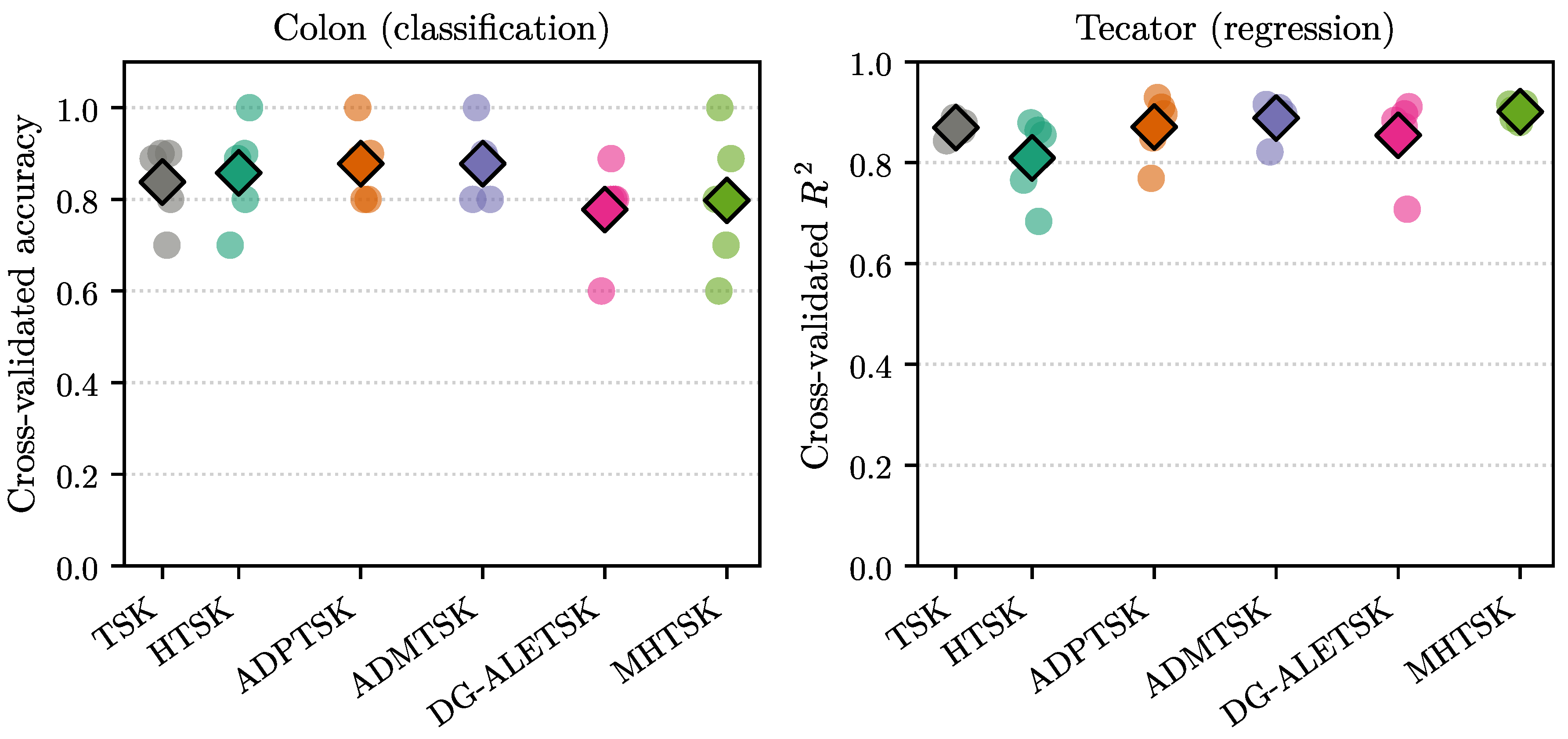
Figure 5.
Out-of-fold diagnostics of the family selected by cross-validation on Colon (ADPTSK), over the 49 training samples, each predicted exactly once by a model fitted without it. Left: the confusion matrix. Right: the decision margin, i.e., the predicted probability of the normal class grouped by true class, with the horizontal bars marking the group means and the dashed line the decision threshold.
Figure 5.
Out-of-fold diagnostics of the family selected by cross-validation on Colon (ADPTSK), over the 49 training samples, each predicted exactly once by a model fitted without it. Left: the confusion matrix. Right: the decision margin, i.e., the predicted probability of the normal class grouped by true class, with the horizontal bars marking the group means and the dashed line the decision threshold.
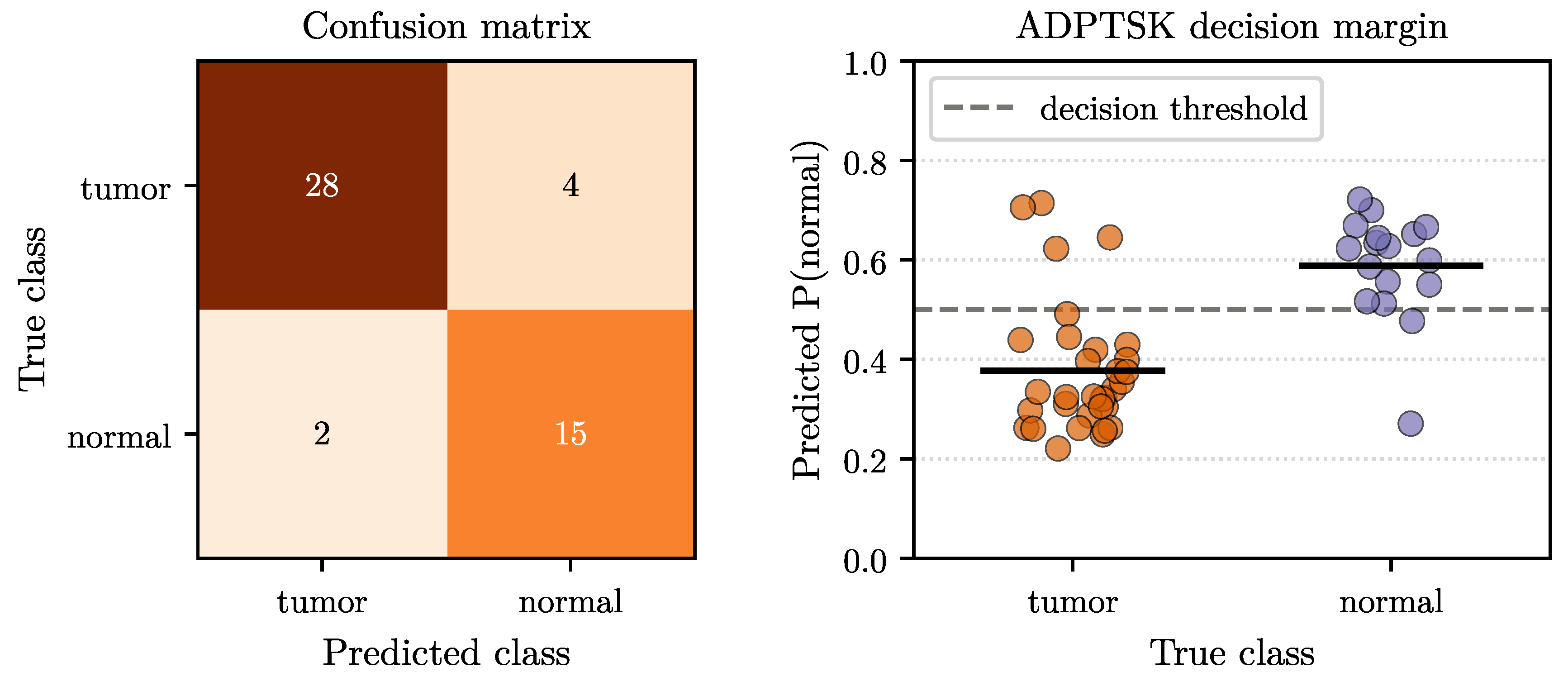
Figure 6.
Two test-set views of the family selected by cross-validation on Tecator (MHTSKRegressor), on the 48 held-out samples. Left: predicted versus observed fat content, with the ideal reference (dashed). Right: residuals (predicted minus observed) against the observed value, with the zero-error reference (dashed); their downward trend shows the fit shrinking toward the mean at the extremes of the range.
Figure 6.
Two test-set views of the family selected by cross-validation on Tecator (MHTSKRegressor), on the 48 held-out samples. Left: predicted versus observed fat content, with the ideal reference (dashed). Right: residuals (predicted minus observed) against the observed value, with the zero-error reference (dashed); their downward trend shows the fit shrinking toward the mean at the extremes of the range.
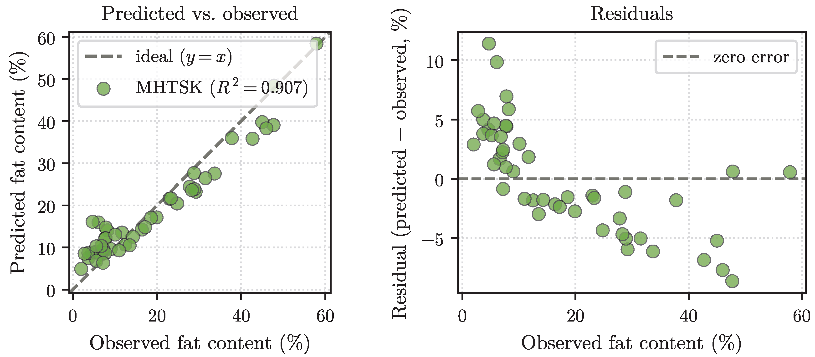

Table 1.
Comparison of open-source Python fuzzy-inference packages. S1–S5 denote the five high-dimensional mitigation strategies of Section 3: (S1) antecedent exponent reformulation, (S2) differentiable softmin approximations, (S3) adaptive parametric T-norms, (S4) structural gating and regularization, and (S5) subspace decomposition. • indicates the feature is present in the package’s source code; “–” indicates it is absent or not applicable. A package that serves both tasks through a single class with a task flag or a user-supplied loss (PyTSK, Scikit-ANFIS, lazuardy-anfis) is marked “–” in the last column, and a fit/predict interface counts as scikit-learn-compatible only when the class derives from scikit-learn’s BaseEstimator. scikit-fuzzy and simpful are Mamdani-oriented libraries without gradient-trained TSK estimators, so the classifier/regressor distinction does not apply to them.
Table 1.
Comparison of open-source Python fuzzy-inference packages. S1–S5 denote the five high-dimensional mitigation strategies of Section 3: (S1) antecedent exponent reformulation, (S2) differentiable softmin approximations, (S3) adaptive parametric T-norms, (S4) structural gating and regularization, and (S5) subspace decomposition. • indicates the feature is present in the package’s source code; “–” indicates it is absent or not applicable. A package that serves both tasks through a single class with a task flag or a user-supplied loss (PyTSK, Scikit-ANFIS, lazuardy-anfis) is marked “–” in the last column, and a fit/predict interface counts as scikit-learn-compatible only when the class derives from scikit-learn’s BaseEstimator. scikit-fuzzy and simpful are Mamdani-oriented libraries without gradient-trained TSK estimators, so the classifier/regressor distinction does not apply to them.
| Package | S1 | S2 | S3 | S4 | S5 | scikit-learn API | GPU backend | Classifier/Regressor |
|---|---|---|---|---|---|---|---|---|
| highFIS | • | • | • | • | • | • | • | • |
| PyTSK [20] | • | – | – | – | – | – | • | – |
| ANFIS-Toolbox [13] | – | – | – | – | – | • | – | • |
| X-ANFIS [16] | – | – | – | – | – | • | • | • |
| ANFISpy [17] | – | – | – | – | – | – | • | – |
| Scikit-ANFIS [19] | – | – | – | – | – | • | – | – |
| lazuardy-anfis [18] | – | – | – | – | – | – | • | – |
| scikit-fuzzy [11] | – | – | – | – | – | – | – | – |
| simpful [12] | – | – | – | – | – | – | – | – |
Table 2.
The classical TSK baseline and the thirteen high-dimensional estimator families implemented in highFIS, grouped by mitigation strategy. AdaTSK and FSRE-ADATSK share the same source reference because FSRE-ADATSK is the feature-selection and rule-extraction extension of the AdaTSK model introduced in the same article.
Table 2.
The classical TSK baseline and the thirteen high-dimensional estimator families implemented in highFIS, grouped by mitigation strategy. AdaTSK and FSRE-ADATSK share the same source reference because FSRE-ADATSK is the feature-selection and rule-extraction extension of the AdaTSK model introduced in the same article.
| Strategy | Family | Estimator classes | Reference |
|---|---|---|---|
| Baseline | TSK | TSKClassifier/TSKRegressor | Takagi and Sugeno [1] |
| Antecedent exponent reformulation (Section 3.1) | |||
| HTSK | HTSKClassifier/HTSKRegressor | Cui et al. [5] | |
| LogTSK | LogTSKClassifier/LogTSKRegressor | Cui et al. [5] | |
| HDFIS-prod | HDFISProdClassifier/HDFISProdRegressor | Xue et al. [6] | |
| HDFIS-min | HDFISMinClassifier/HDFISMinRegressor | Xue et al. [6] | |
| Differentiable softmin approximations (Section 3.2) | |||
| AdaTSK | ADATSKClassifier/ADATSKRegressor | Xue et al. [7] | |
| ADPTSK | ADPTSKClassifier/ADPTSKRegressor | Ma et al. [3] | |
| Adaptive parametric T-norms (Section 3.3) | |||
| DombiTSK | DombiTSKClassifier/DombiTSKRegressor | Xue et al. [2] | |
| ADMTSK | ADMTSKClassifier/ADMTSKRegressor | Xue et al. [2] | |
| AYATSK | AYATSKClassifier/AYATSKRegressor | Xue et al. [8] | |
| Structural gating and regularization (Section 3.4) | |||
| DG-TSK | DGTSKClassifier/DGTSKRegressor | Xue et al. [9] | |
| DG-ALETSK | DGALETSKClassifier/DGALETSKRegressor | Xue et al. [10] | |
| FSRE-ADATSK | FSREADATSKClassifier/FSREADATSKRegressor | Xue et al. [7] | |
| Subspace decomposition (Section 3.5) | |||
| MHTSK | MHTSKClassifier/MHTSKRegressor | Bian et al. [4] | |
Table 3.
Principal configuration arguments shared by the highFIS estimators, with defaults for the baseline families. Some families adjust individual defaults: LogTSK, DombiTSK, the HDFIS, DG-TSK, and DG-ALETSK families, and FSRE-ADATSK use n_mfs = 5. The rule_base default is resolved from mf_init: grid initialization defaults to "cartesian" and clustering initialization to "coco". With batch_size = "auto", each family uses the batch-size protocol of its source article, resolved from the number of training samples when fit() is called.
Table 3.
Principal configuration arguments shared by the highFIS estimators, with defaults for the baseline families. Some families adjust individual defaults: LogTSK, DombiTSK, the HDFIS, DG-TSK, and DG-ALETSK families, and FSRE-ADATSK use n_mfs = 5. The rule_base default is resolved from mf_init: grid initialization defaults to "cartesian" and clustering initialization to "coco". With batch_size = "auto", each family uses the batch-size protocol of its source article, resolved from the number of training samples when fit() is called.
| Argument | Options | Default | Effect |
|---|---|---|---|
| n_mfs | int | 3 | Number of fuzzy sets per input feature |
| mf_init | "grid", "kmeans", "fcm", clusterer | "kmeans" | Membership-center initialization strategy |
| sigma_scale | float, "auto" | 1.0 | Initial spread scaling ("auto" ) |
| rule_base | "cartesian", "coco", "pfrb" | init-dependent | Rule combination scheme and rule count |
| epochs | int | 100 | Number of gradient training passes |
| learning_rate | float | 0.01 | Optimizer step size |
| weight_decay | float | 1e-8 | L2 penalty on the consequents only |
| patience | int, None | 20 | Early-stopping patience in epochs |
| batch_size | int, None, "auto" | "auto" | Mini-batch size (None = full batch) |
| ur_weight | float | 0.0 | Weight of the uniform regularization (UR) term |
| device | "cpu", "cuda", "mps" | "cpu" | PyTorch compute backend |
Disclaimer/Publisher’s Note: The statements, opinions and data contained in all publications are solely those of the individual author(s) and contributor(s) and not of MDPI and/or the editor(s). MDPI and/or the editor(s) disclaim responsibility for any injury to people or property resulting from any ideas, methods, instructions or products referred to in the content. |
© 2026 by the authors. Licensee MDPI, Basel, Switzerland. This article is an open access article distributed under the terms and conditions of the Creative Commons Attribution (CC BY) license (http://creativecommons.org/licenses/by/4.0/).
Copyright: This open access article is published under a Creative Commons CC BY 4.0 license, which permit the free download, distribution, and reuse, provided that the author and preprint are cited in any reuse.