

Submitted:
03 October 2026
Posted:
07 October 2026
You are already at the latest version
Abstract
Objective. Deep brain stimulators, cardiac pacemakers, cochlear implants and transcutaneous nerve stimulators all deliver the same rectangular industrial pulse across target tissues that differ by several orders of magnitude in electrical conductivity. This shape was inherited from 1970s electronics rather than being chosen on physiological grounds. This paper establishes a quantitative electrical benchmark for comparing candidate waveforms on spectral, energetic and hardware axes, which is a prerequisite to any fibre-level analysis. Approach. Eight waveforms, including the industrial rectangle and its clinical asymmetric variant, as well as a smooth curve, are driven through equivalent circuit models of eight target tissues, which cover the clinical conductivity range. Each tissue is represented by a linear passive network fitted to its measured dielectric spectrum, and every waveform-tissue pair is solved in the time domain under voltage- and current-driven modes. Main results. The smooth curve outperforms the industrial rectangle by two to three orders of magnitude on spectral leakage, and requires approximately ninety times less peak current per unit of delivered charge. On peak tissue voltage, tissue impedance dominates the ordering. The asymmetric rectangle sits at the opposite end of the ordering. Spectral rankings are invariant to drive mode, while peak tissue voltage varies in magnitude across tissues at a fixed clinical dose. Significance. Smooth-waveform alternatives to the industrial rectangle could reduce the peak current, thermal and battery demands of neural implants by up to two orders of magnitude, while maintaining the delivered charge. This would open up a design margin that is currently unavailable to clinicians and device makers. For patients receiving a chronic implant, this translates directly into longer intervals between battery-replacement surgeries at equal clinical dose.
Keywords:
computer simulation
; deep brain stimulation
; electric impedance
; electric stimulation therapy
; fourier analysis
1. Introduction
A clinician switches on a deep brain stimulator. The pulse leaving the generator is a rectangle: 600 of positive voltage, 600 of negative voltage, repeated at about 130 [1,2]. Three other clinical technologies deliver the same class of waveform to different target tissues. The cardiac pacemaker, implanted since 1958, applies a rectangular biphasic pulse to the myocardium to pace a failing heart [3]. The cochlear implant, in continuous clinical use since the 1960s, applies a rectangular biphasic pulse via the cerebrospinal fluid to excite the spiral ganglion neurons [4]. The transcutaneous electrical nerve stimulator, popularised in the 1970s, applies a rectangular biphasic pulse through the skin to activate afferent nerve fibres [5]. Four applications, four target tissues, four decades of history, one waveform.
The four target tissues differ by four orders of magnitude in their DC ionic conductivity, from about 2Sm−1 in cerebrospinal fluid down to about 2 × 10⁻⁴ Sm−1 in skin. That the same rectangular pulse should be an appropriate stimulus across such a range of electrical environments has not been argued on physical or physiological grounds.
The shape was chosen for what it made easy: the silicon of the 1950s to 1970s could deliver a rectangle and little else. It has been the industrial standard ever since. Since 2010, several groups have proposed alternative shapes on various grounds: energy efficiency [6,7], spectral properties [8,9], fibre-level modelling [2,10,11], and empirical demonstrations at the network level [12]. The convergent thread is that the rectangle is a legacy shape and not an optimised one.
The literature does not yet supply a common ground on which existing and future waveforms can be compared. Each proposal has been tested on a different tissue, a different electrode geometry, and a different metric. A reader who asks how these waveforms compare across the tissues that matter clinically, and on which axis, has no unified answer.
This paper provides that common ground. Eight candidate waveforms are driven through equivalent circuit models of eight target tissues drawn from the clinical range: nerve, skin, heart muscle, cerebrospinal fluid, muscle, bone, fat, and blood. Each tissue is represented by a passive network calibrated to its measured electrical properties, as tabulated in Gabriel et al. [13]. The eight waveforms are compared on four axes: how their energy is spread across frequencies, how that energy is split between resistive and dielectric dissipation, how much peak current is required to deliver a given dose, and whether the response settles to a clean periodic regime. The measurement-based posture aligns with the growing methodological consensus in electrical stimulation [10,14].
Two observations from the ranking deserve early mention. The exponential decay, sometimes described as a softened rectangle, turns out worse than the rectangle on the spectral axis. The rectangle with an interphase gap turns out better than the plain one. Both observations follow from the derivative of the pulse train, and both suggest that the rectangle is not close to any local optimum. The rest of the ordering, and the tissue dependence of its magnitudes, is quantified in what follows. In plainer terms, the question the paper puts is: why should the stimulus carry frequency harmonics for which no clinical benefit has been established, and which the electrode-tissue interface pays for in heat and stress?
2. Materials and Methods
2.1. The Eight Tissues We Tested
To test a stimulation waveform we need something to stimulate. We chose a panel of eight target tissues, picked to be as different from each other as possible while remaining relevant to clinical practice. At one extreme sits cerebrospinal fluid, which behaves almost like salt water: it lets electricity through with barely any loss. At the other extreme sits dry skin, whose stack of dead cells opposes the passage of current across the entire audio range and beyond. Between the two we placed blood, muscle, heart muscle, bone, nerve, and fat. Ordered by electrical conductivity, the panel spans four orders of magnitude from the most conductive to the least, and covers the neural, epithelial, muscular, connective, and fluid tissue categories that a clinician typically encounters.
Each tissue is fully described by fourteen numbers that fit its dielectric behaviour to a widely used four-dispersion model, sometimes called the Cole–Cole model, discussed in Appendix A. The values we used come from version 5.0 of the database maintained by the IT’IS Foundation [15], itself a curated extension of the original spectroscopy measurements of Gabriel et al. [13,16,17]. We cross-checked the tabulated numbers against Table 1 of Gabriel et al. [13] and against the online calculator of the IFAC-CNR [18], at two representative frequencies. Agreement was within numerical precision at both check points.
For every tissue in the panel, the electrical properties we care about are captured by two convenient numbers: the DC ionic conductivity and the resulting DC resistance of a reference slab of 1 cm2 by 1 thick. These two numbers are listed in Table 1, tissue by tissue. The full fourteen-parameter description of each tissue serves the equivalent-circuit construction of the next subsection.

Table 1.
The eight tissues of the testbed, ordered by DC ionic conductivity, from the most conductive to the least. Reference geometry: cross-section , thickness . Cole–Cole parameters from IT’IS Foundation V5.0, itself a curated extension of Gabriel et al. [13].
Table 1.
The eight tissues of the testbed, ordered by DC ionic conductivity, from the most conductive to the least. Reference geometry: cross-section , thickness . Cole–Cole parameters from IT’IS Foundation V5.0, itself a curated extension of Gabriel et al. [13].
| Tissue | (Sm−1) | (Ω) |
|---|---|---|
| Cerebrospinal fluid | 2.0 | 5 |
| Blood | 0.7 | 14.3 |
| Muscle | 0.2 | 50 |
| Heart muscle | 0.05 | 200 |
| Bone (cortical) | 0.02 | 500 |
| Fat (not infiltrated) | 0.01 | 1000 |
| Nerve | 0.006 | 1667 |
| Skin | 2 × 10⁻⁴ | 50000 |
2.2. Building a Circuit that Behaves like Each Tissue
The dielectric model of the tissue lives in the frequency domain: it tells us what the tissue does when we shake it with a sine wave, at each frequency. The simulator we use, ngspice, lives in the time domain: it tells us what the tissue does moment by moment, when we drive it with any voltage waveform we like. Bridging the two requires a bit of translation.
The translation is a Foster network: a family of resistors and capacitors connected in a specific pattern, whose collective behaviour matches the frequency-domain response of the tissue over the range we care about. The details of the pattern, and of the fitting procedure that assigns numerical values to every resistor and capacitor, are given in Appendix A. What matters here is that we can build one such network for each of our eight tissues, and drop each network into a circuit simulator as a two-terminal block.
The construction fits the frequency-domain response to within two per cent of relative error, for twenty-five of the twenty-six non-degenerate dispersions of the panel. The one exception is a slow dispersion of Fat (not infiltrated), which fits at 3.25 per cent. That single residual has no effect on the transient results we present, as we verify later in the discussion of limitations.
2.3. The Eight Candidate Waveforms
Eight waveforms enter the ring. All are biphasic and charge-balanced, all reach a peak amplitude of on their primary phase with in the voltage-driven campaign, all finish their active phases within 1200 , and all repeat every 15 . Table 2 lists their per-phase parameters and clinical anchors, and Figure 1 draws the eight shapes overlaid.
The eighth candidate is one we introduce here, with clinical intent as its design driver. A sharp waveform places most of its energy at high frequencies, where the tissue absorbs it as heat and interface stress rather than as fibre excitation; a smooth waveform delivers the same charge with a spectrum concentrated in the low-frequency band that actually drives the fibre, sparing the tissue of the excess. We call it the slope-continuous biphasic waveform (SCB), naming it after the property that defines it rather than after the curve family used to build it. The shape is a smooth cubic curve built from three concatenated Bézier segments, joined so that value and slope match at every junction; it is this continuity of the first derivative, and not the cubic parametrisation as such, that governs the spectral behaviour reported below. The construction and the numerical procedure that enforces zero net charge are spelled out in Appendix B. The curve is deliberately asymmetric in time: a fast rise, followed by a slow relaxation that carries a controlled hyperpolarisation dwell, mirroring the shape a neural excitation naturally takes.
Figure 1.
The eight candidate waveforms, shown on the first 11 ms of the period, at unit peak amplitude on the primary phase. The same shape drives the two campaigns: the voltage-driven campaign scales the shape to ; the current-driven campaign scales it to a per-cell current amplitude calibrated so that the total delivered charge matches, cell by cell, the value of the corresponding voltage-driven run (Section 2.4). All eight are positive-first, period , remainder of the period at zero.
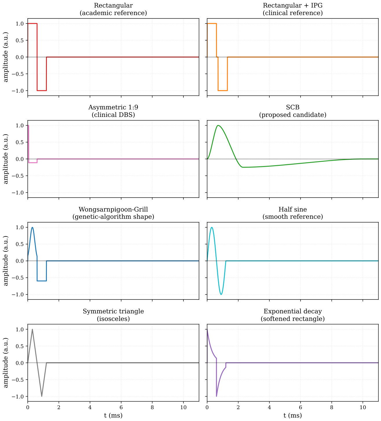
Table 2.
The eight candidate waveforms of the campaign. Positive phase and negative phase columns describe the shape and duration of each active phase on the primary window. Interphase gaps are noted inline in the negative phase column when present. All waveforms are biphasic and charge-balanced on the period T = 15 ms; the remainder of the period is at zero. Peak amplitude on the primary phase is , with V = 1 V in the voltage-driven campaign.
| Waveform | Positive phase | Negative phase | Clinical or historical anchor |
|---|---|---|---|
| Rectangular biphasic (Rect) | 600 at | 600 at | industrial standard |
| Rectangular + interphase gap | 600 at | 600 at , after a 100 silence | DBS and cochlear implants [1,4] |
| Rectangular asymmetric 1:9 | 60 at | 540 at | modern DBS, Lilly family [1,2,19] |
| Wongsarnpigoon–Grill | 600 Gaussian centred at , scale | 600 rectangular at | energy-optimal, genetic algorithm [6] |
| Half sine | 600 half-sine at | 600 half-sine at | industrial reference (LCR meters, network analysers) |
| Exponential decay | 600 , exponential decay from | 600 , exponential decay from | “softened rectangle” |
| Symmetric triangle | 300 rise then 300 fall, peak | mirror at | zero at every phase boundary |
| Slope-continuous biphasic (SCB) | 700 rise to | 1.5 descent through zero to a hyperpolarisation trough near , then 8 relaxation to zero | proposed here, see next paragraph |
2.4. How the Simulation Runs
The benchmark runs in two operating modes, both of which are sketched in Figure 2. In each mode, every combination of one waveform and one tissue circuit is fed through one hundred periods in a row, so that any initial transient dies out and only the steady-state response remains at the end. We record the last of the hundred periods for analysis.
In the voltage-driven configuration (Figure 2(a)), the source is an ideal voltage source that reproduces the candidate waveform on the interval with . A series resistor between the source and the tissue models the finite output impedance of a real stimulator. This configuration matches the majority of the neurostimulation waveform benchmark literature and is directly comparable to our earlier campaigns on this pipeline.
In the current-driven configuration (Figure 2(b)), the source is an ideal current source with infinite output impedance, following the NEURON IClamp convention [20,21] that is the standard in the fibre-model community our benchmark is meant to inform. The waveform shape is the one of the voltage-driven case, and the amplitude of is calibrated per (tissue, waveform) cell so that the total delivered charge per phase, , matches, to a numerical residual below one per cent, the value recorded in the corresponding voltage-driven run. This isocharge calibration is what makes the two campaigns comparable on the four benchmark axes; the cell-by-cell comparison itself is the object of Section 3.8.
Figure 2.
The driven circuit, in both operating modes. (a) voltage-driven: a voltage source delivers the candidate waveform through a 50 Ω resistor that models the stimulator output impedance, and the tissue block is one of the eight Foster networks; we monitor the voltage at the tissue terminals and the current through the source. (b) current-driven: an ideal current source delivers the calibrated waveform at strictly matched delivered charge, and a zero-volt ammeter placed between nodes a and b measures , the physical current entering the tissue at node b; is absent, following the NEURON IClamp convention [20,21]. The tissue Foster subcircuit is identical in the two panels.
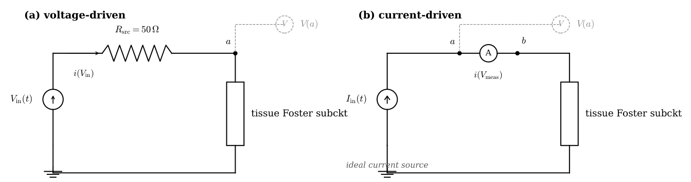
The simulator is ngspice [22], an open-source circuit solver that has been under active maintenance for more than a decade. The mundane details of the input format, the transient output ordering and the way the waveform is emitted as a piecewise-linear inline function are collected in Appendix C. We flag two conventions on the current column reported by ngspice that matter for interpretation. In the voltage-driven configuration, ngspice reports the current through with its own internal convention, which is opposite to the physical current entering the tissue as a load; we flip the sign on read so that positive current means current flowing into the tissue from the anode, which is what a clinician expects to see. In the current-driven configuration, the zero-volt ammeter is oriented from node a to node b with a upstream of the tissue, and its current is read with the physical convention already applied, positive when it flows from a through and enters the tissue at node b; no sign flip is required on read.
2.5. Four Ways to Look at the Result
From the last-period trace of each simulation we extract four kinds of information about the stimulus-tissue combination. Each of the four illuminates a different aspect of the interaction. The exact mathematical definitions of the four are collected in Appendix D; in the body of the paper we work with the physical intuition of each quantity.
Charge
How much positive charge went in during the positive phase, how much negative charge came out during the negative phase, and how well the two balance. A strictly steady-state cycle balances them exactly. A residual imbalance says that the transient has not fully decayed, or in more capacitive tissues, that the relaxation time of one slow dispersion exceeds the simulated duration.
Energy
Every joule delivered by the stimulator is absorbed by the tissue. Only a fraction of it contributes to fibre excitation: the low-frequency component the fibre actually responds to. The remainder is dissipated as heat inside the tissue and as stress at the electrode-tissue interface, without any clinical benefit and at direct cost to battery life and to the electrode itself. Two physical paths carry this dissipation, one through the tissue’s conductive properties and one through its dielectric relaxation, and the ratio of the two labels the regime of the tissue-waveform combination as conductive-dominant, dielectric-dominant, or mixed. The mathematical definitions and the branch-by-branch numerical computation are collected in Appendix D.
Peaks
The rectangle sends its whole charge through a very short window; the smoother waveforms spread the same charge over longer intervals. To deliver the same clinical dose (the same total charge per phase), the rectangle therefore requires a stimulator that can swing a much higher peak current than the smooth waveforms. We record the peak absolute current and the peak current divided by the delivered charge, as a measure of the hardware demand.
Where the Energy Sits in Frequency
We use a reference cutoff of 2 to separate the spectral content of the applied waveform into two bands: a useful band from DC to the cutoff, and an out-of-band tail above it. The choice of 2 is motivated by the characteristic activation time of sodium channels in myelinated mammalian axons, approximately 500 . Energy delivered above this cutoff does not contribute efficiently to fibre-level excitation and is likely to load the tissue and its interface for no useful physiological return. We compute the fraction of the voltage energy and the fraction of the current energy that fall outside this useful band on the last period.
3. Results
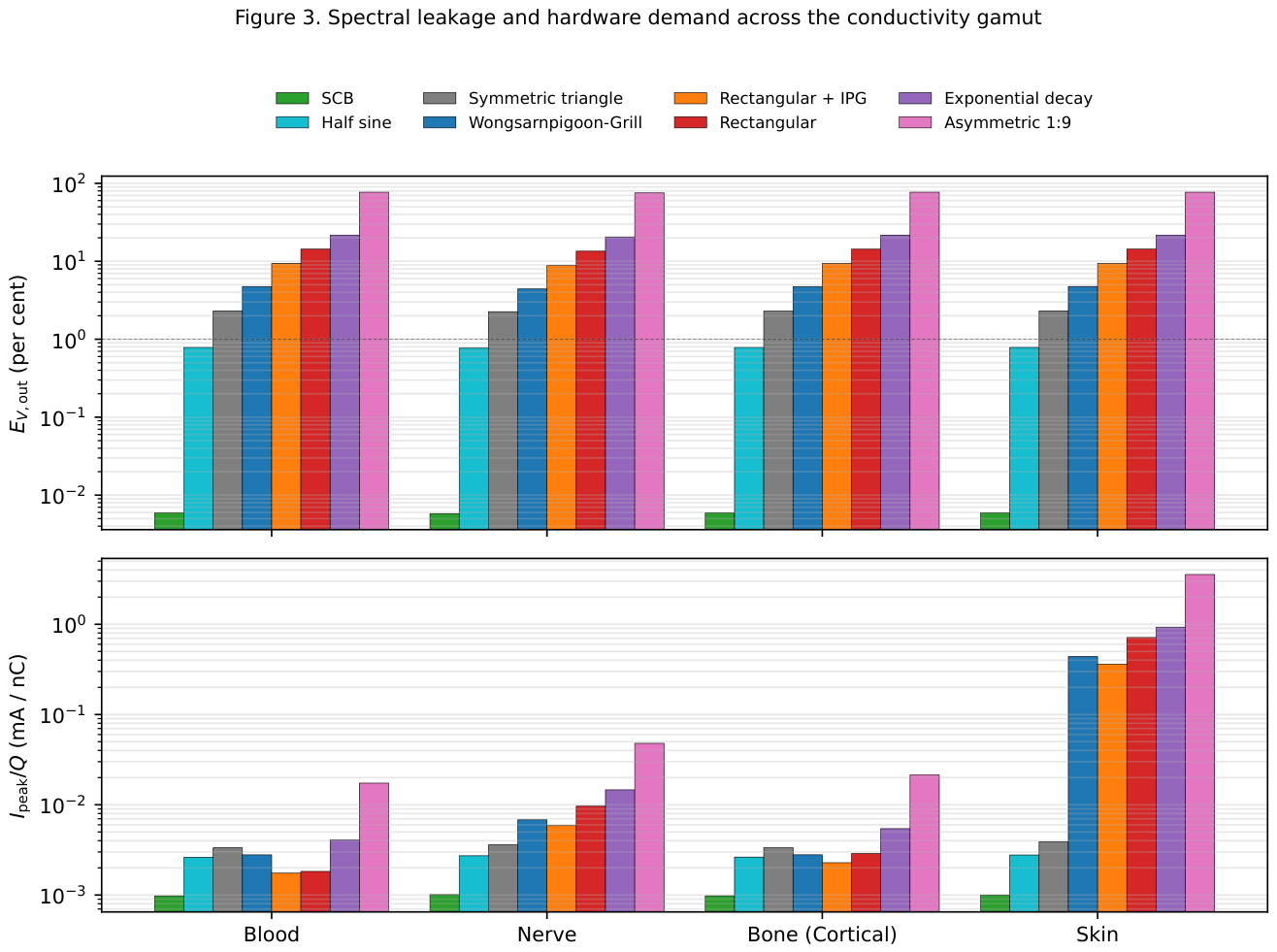
Each combination of waveform and tissue produces a last-period trace, from which we extract the four quantities described in Section 2.5. Sixty-four combinations produce a data set that we now walk through, axis by axis. Figure 3 summarises the two axes on which the eight waveforms are most cleanly separated, on four representative tissues of the conductivity gamut. Figure 4 and Figure 5 zoom on Skin, the most instructive single tissue.
Figure 3.
Spectral leakage and hardware demand across the conductivity gamut. Top: fraction of the terminal voltage energy that leaks above 2 kHz, in per cent, on four tissues spanning four decades of DC ionic conductivity (Blood, Nerve, Bone (cortical), Skin). Bottom: peak absolute current per unit delivered charge, in milliamperes per nanocoulomb. Both axes are shown on a base-ten logarithmic scale. Waveforms in the same colour code as Figure 1.
3.1. Spectral Leakage at the Tissue Terminals
The tissue does not respond equally to every frequency contained in the applied waveform. The part below 2 drives fibre excitation; the part above it does not, and simply loads the tissue and its electrode interface for no clinical benefit. The wasted fraction, which we call spectral leakage, varies widely across the eight waveforms. Table 3 lists its tissue-averaged value, in increasing order.
Table 3.
Out-of-band voltage energy fraction , averaged across the eight tissues, for the eight candidate waveforms, in increasing order.
Table 3.
Out-of-band voltage energy fraction , averaged across the eight tissues, for the eight candidate waveforms, in increasing order.
| Waveform | (%) |
|---|---|
| SCB | 0.006 |
| Half sine | 0.77 |
| Symmetric triangle | 2.24 |
| Wongsarnpigoon–Grill | 4.54 |
| Rectangular + interphase gap | 9.00 |
| Rectangular biphasic | 13.76 |
| Exponential decay | 20.91 |
| Rectangular asymmetric 1:9 | 76.06 |
Four of these results deserve a pause.
The rectangle with an interphase gap performs better than the plain rectangle, not worse. The gap, 100 of silence between the two active phases, splits what would otherwise be a single abrupt swing of 2 into two smaller swings of 1 each. Two small swings cost the tissue less than one big swing, for the same delivered charge. The quantitative reason (the high-frequency cost scales with the square of the swing) is collected in Appendix D.
The exponential decay performs worse than the rectangle it was supposed to soften. The reason is that its cathodic phase never reaches zero: at the end of the phase, the voltage still sits at about a third of its starting value, and then jumps abruptly to the opposite polarity. That leftover jump is larger than the swings of the plain rectangle, and drives the leakage up.
The symmetric triangle performs six times better than the plain rectangle, at 2.24 per cent against 13.76 per cent, and better even than the Wongsarnpigoon–Grill waveform at 4.54 per cent. The improvement is not obtained by smoothing the interior of each phase, which remains a straight ramp with a sharp peak, but by having the waveform meet zero at every phase boundary: at the start, at the mid-point where cathode changes to anode, and at the end. What matters for spectral cost is therefore whether the waveform lands on zero at each junction, not whether it is smooth in between. We return to this point in the discussion below.
The asymmetric 1:9 rectangle sits at the far end of the ordering, at 76 per cent. Its short cathodic phase, 60 long, concentrates the entire delivered charge into a spike ten times shorter than the reference phase duration. Compressing the same charge into a tenth of the time pushes essentially all of the delivered energy above the useful band. The shape is asymmetric in time and, as we shall see, catastrophic on every other axis of the benchmark.
One further observation reads less naturally from the numbers but shows up clearly on Figure 3: the spectral leakage at the tissue terminals varies by less than one percentage point across the eight tissues, for each of the seven non-asymmetric waveforms. The reason is straightforward. In the useful band and immediately above it, the eight tissues all behave essentially as resistors: they oppose the current with a resistance that hardly depends on frequency. The voltage delivered at the tissue terminals is therefore, to a very good approximation, the applied waveform itself. Spectral leakage at the terminals is spectral leakage of the applied waveform, whatever the tissue.
3.2. Spectral Leakage in the Delivered Current
The current entering the tissue behaves very differently. Unlike the voltage, which the tissue receives essentially unchanged, the current is shaped by whatever passive network the tissue happens to be. A capacitive tissue lets high-frequency current through; a resistive tissue lets the current match the voltage waveform.
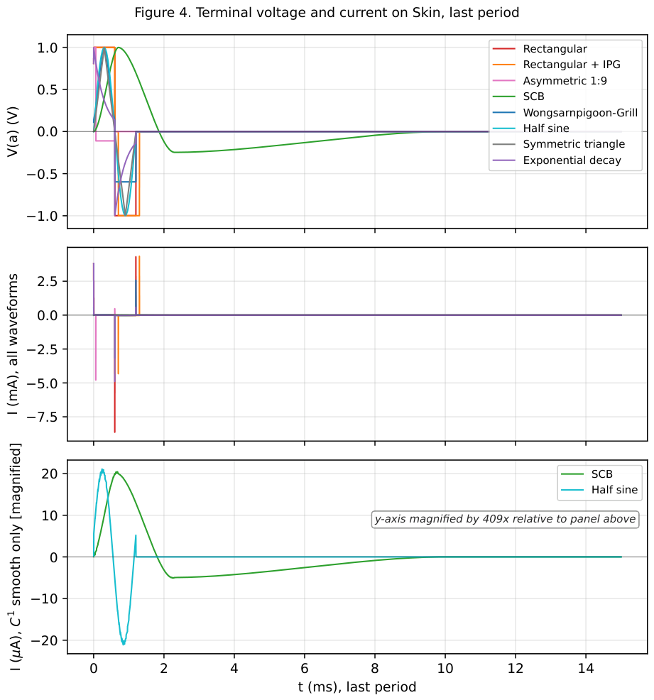
The contrast is starkest on Skin, which behaves like a capacitor across most of the useful band. On Skin, current only appears when the voltage moves: a train of sharp spikes at each voltage transition, and virtually nothing between them. Table 4 lists the out-of-band fraction of the delivered current energy on Skin for the eight waveforms. Under a rectangular waveform, ninety-seven per cent of the current energy sits above 2 ; under the SCB, that fraction drops to 0.01 per cent, four orders of magnitude below.
Table 4.
Out-of-band current energy fraction on Skin, for the eight candidate waveforms, in increasing order. Skin is the most capacitive tissue of the panel and separates the waveforms most sharply; the pattern attenuates on tissues less capacitive than Skin (see body text).
Table 4.
Out-of-band current energy fraction on Skin, for the eight candidate waveforms, in increasing order. Skin is the most capacitive tissue of the panel and separates the waveforms most sharply; the pattern attenuates on tissues less capacitive than Skin (see body text).
| Waveform | on Skin (%) |
|---|---|
| SCB | 0.011 |
| Half sine | 1.44 |
| Symmetric triangle | 4.01 |
| Wongsarnpigoon–Grill | 92.80 |
| Rectangular + interphase gap | 95.50 |
| Rectangular biphasic | 97.34 |
| Exponential decay | 98.39 |
| Rectangular asymmetric 1:9 | 99.92 |
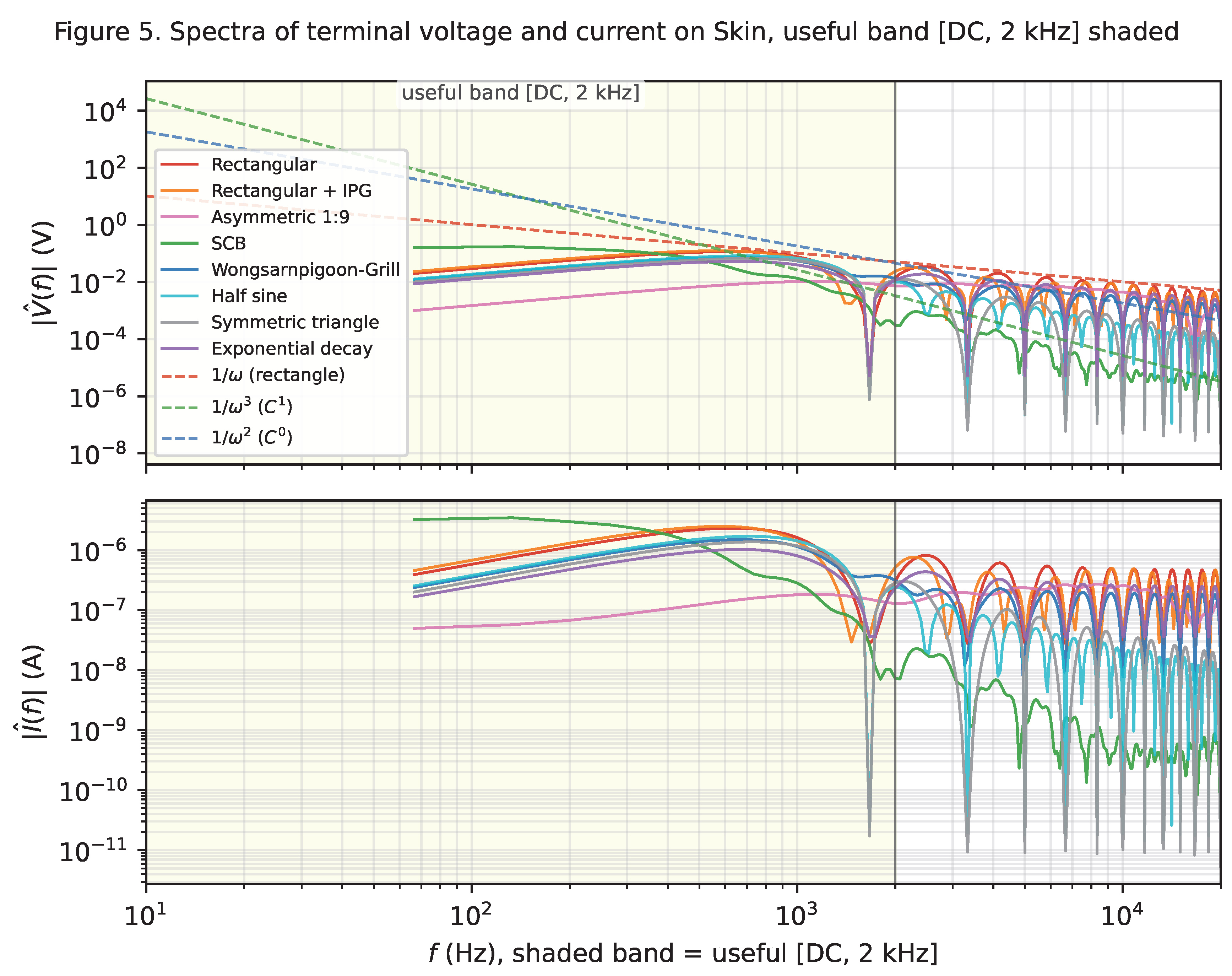
Figure 4 and Figure 5 show the effect directly. On the top-right panel, the plain rectangle produces two sharp current spikes of about 5 each at the two voltage edges, with a floor of a few tens of microamperes elsewhere. The SCB produces a slowly varying current of a few tens of microamperes throughout. Same delivered charge; entirely different current signature.
Figure 4.
Skin under the eight candidate waveforms, temporal view of the last period. Top: voltage at the tissue terminals, all eight waveforms. Middle: current I through the source, all eight waveforms, milliampere scale. Bottom: same current restricted to the two smooth candidates (SCB and half sine), on a microampere scale magnified about four hundred times relative to the middle panel.
On tissues that are less capacitive than Skin, this contrast attenuates but does not disappear. On Nerve, the plain rectangle leaks 23 per cent of its current energy above 2 , and the SCB again 0.01 per cent. On Blood, which is essentially resistive, the current follows the voltage waveform and the spectral leakage of the current matches that of the voltage to within a percentage point. The general rule is that the more capacitive the tissue, the more the current leakage exceeds the voltage leakage.
An observation specific to the Wongsarnpigoon–Grill waveform deserves mention here. On seven of the eight tissues in the panel, the truncated Gaussian delivers less than two per cent of its current energy above the useful band. On Skin, this figure jumps to 46 per cent. The reason is the small residual step of about a tenth of the peak voltage that the truncated Gaussian leaves at the start and end of each active phase: its exponential envelope does not quite reach zero at the phase boundary. Seven of the eight tissues are not capacitive enough to detect the step; Skin, which responds only to transitions, turns it into a wideband current burst. Skin thus acts as a sensitivity test that reveals residual jumps invisible on the other tissues in the panel.
Two related observations extend the pattern to the triangle and to the asymmetric 1:9 rectangle. The symmetric triangle on Skin leaks only 4.0 per cent of its current energy above the useful band, a value close to its 2.3 per cent on all other tissues in the panel and a factor of twelve better than the Wongsarnpigoon–Grill waveform on the same tissue. Skin no longer reveals a residual jump, because the triangle has none in value; its two slope changes at the peaks are gentle enough to stay inside the useful band, and Skin’s response never enters the wideband regime. The asymmetric 1:9 rectangle, in turn, sits at 99.9 per cent on Skin: its short cathodic phase concentrates the entire charge into 60 , and Skin, which responds only to transitions, amplifies this into a wideband current spike whose peak reaches several milliamperes for a target charge in the nanocoulomb range.
Figure 5.
Skin under the eight candidate waveforms, spectral view. Top: magnitude spectrum at the tissue terminals. Bottom: magnitude spectrum of the source current. The useful band [DC, 2 kHz] is shaded.
Figure 5.
Skin under the eight candidate waveforms, spectral view. Top: magnitude spectrum at the tissue terminals. Bottom: magnitude spectrum of the source current. The useful band [DC, 2 kHz] is shaded.
3.3. Bulk Conductive and Dielectric Energy Shares
Every joule the stimulator delivers to the tissue leaves it as heat, along one of two paths. One path is ordinary ohmic dissipation, following the tissue’s ionic conduction: we call this the bulk conductive contribution, and it is what the stimulus intends. The other path is dissipation associated with the frequency-dependent polarisation of the water, membranes and macromolecules that surround the ionic paths: we call this the dielectric contribution, and it is not directly intended.
The ratio of the two changes from one tissue to the next, on the same applied waveform, across four orders of magnitude. Nerve sits at a ratio of about 0.25: its dielectric contribution dissipates roughly four times as much energy as its ionic conduction, on any of the eight waveforms. Fat, Heart muscle and Muscle occupy a mixed regime between one and about two, in which the two contributions are comparable. Bone (cortical) sits between about a hundred and three hundred, dominated by its ionic conduction. Blood and Cerebrospinal fluid are essentially pure resistors on this stimulus: their dielectric contribution falls below what the simulator can resolve, and the ratio sits at the numerical ceiling of ten thousand.
The waveform axis modulates it, but the tissue axis dominates, and the four-decade tissue gamut of the ratio is a property of the panel, not of the stimulus.
3.4. Peak Current Per Unit Delivered Charge
A stimulator has to swing a certain peak current to deliver a target charge. The peak current sets the maximum output rating of the driver, the width of the H-bridge transistors, and the average battery drain in a chronic implant. It is a hardware axis, and it separates the eight waveforms cleanly.
Table 5 lists the peak absolute current per unit delivered charge, averaged across the eight tissues, for the eight candidate waveforms. The range spans nearly three decades, from about 1 nC−1 for the SCB to 466 nC−1 for the asymmetric 1:9 rectangle.
Table 5.
Peak absolute current per unit delivered charge, , averaged across the eight tissues, for the eight candidate waveforms, in increasing order.
Table 5.
Peak absolute current per unit delivered charge, , averaged across the eight tissues, for the eight candidate waveforms, in increasing order.
| Waveform | (μA nC−1) |
|---|---|
| SCB | 1.0 |
| Half sine | 2.7 |
| Symmetric triangle | 3.5 |
| Rectangular + interphase gap | 47.7 |
| Wongsarnpigoon–Grill | 57.9 |
| Rectangular biphasic | 92.4 |
| Exponential decay | 121.9 |
| Rectangular asymmetric 1:9 | 466.3 |
The last of these deserves comment. The asymmetric 1:9 rectangle demands roughly five times the peak current of the plain rectangle for the same delivered charge. Its short cathodic phase concentrates the entire charge into 60 , and the resulting peak swings past several milliamperes.
The bottom panel of Figure 3 plots the peak current per unit charge for every combination on the four representative tissues, and reads as a hardware brief. For the same clinical dose, an SCB waveform relaxes the peak current requirement of the stimulator by about two decades relative to the plain rectangle and by nearly three decades relative to the asymmetric 1:9 rectangle, on every tissue tested. The stimulator can be smaller, cheaper, and (if chronically implanted) last longer between battery replacements or wireless recharges.
3.5. Peak Tissue Voltage
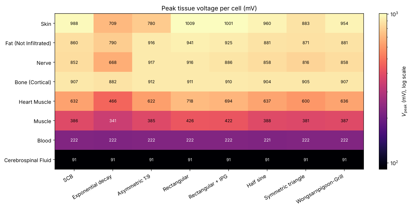
The peak absolute voltage at the tissue terminals on the last period, , quantifies the electrical stress that the stimulus puts on the tissue at each cycle. It is complementary to the peak current of Section 3.4: a stimulator can be sized to deliver a target charge in many ways, and different sizings put different peaks on the two axes. Figure 6 reports for the sixty-four cells of the current-driven campaign at the reference amplitude used throughout the paper. Two properties of the map are worth noting.
Firstly, the tissue axis dominates. On the same waveform, ranges from about 90 on Cerebrospinal fluid to about 1 on Skin, over one order of magnitude. This ordering tracks the tissue’s DC resistance across the panel: the low-resistance tissues (Blood, Cerebrospinal fluid) develop only a fraction of the source amplitude at the port, while the high-resistance tissues (Skin, Bone (cortical), Fat, Nerve) reach values close to the source amplitude on most waveforms. On the same tissue, the modulation from one waveform to the next stays within a factor of about 1.5. Bone (cortical) is a notable outlier on this second front: its varies by less than 30 across the eight waveforms and stays above 880 throughout, making it the tissue that receives the most sustained voltage stress regardless of waveform choice, even though its single-cell maximum (912 ) sits below Skin’s ( 1009 ).
Secondly, the waveform axis is nearly opposite to the peak-current axis of Section 3.4. On every dispersive tissue of the panel, the exponential decay biphasic waveform gives the lowest , the symmetric triangle sits just above it, the SCB and asymmetric 1:9 rectangle occupy the middle third, and the rectangular family closes the ordering at the highest . Physically, the tissue’s capacitive polarisation absorbs sharp current transitions and lets sustained current plateaus force the port voltage to build up cycle after cycle: exponential decay concentrates its current in a fast initial spike that the tissue absorbs efficiently; the rectangular family sustains a constant current across the full phase duration, which the tissue cannot absorb, and which forces the port voltage to keep rising.
The consequence for waveform choice is direct. No single waveform dominates both peak-current and peak-voltage axes. The SCB keeps peak current and spectral leakage low, at the cost of a middle-tier position on peak voltage; the exponential decay does the opposite. The rectangular family is dominated on every other axis and is not competitive on peak voltage either. The tissue axis, again, decides the absolute value: at the reference source amplitude of 1 , the six dispersive tissues sit at values in the range 0.4 V to 1.0 V. The ordering of waveforms on this axis is preserved between the two drive modes, from the exponential decay biphasic at the low end to the rectangular family at the high end on every dispersive tissue. The absolute values differ on the high-impedance tissues (Skin, Fat, Nerve, Bone (cortical)). In voltage-driven mode, is pinned close to the source amplitude for every waveform, because the 50 source impedance is negligible against the tissue impedance. In current-driven mode, reported in Figure 6, the waveforms separate cleanly by their spectral shape.
Figure 6.
Peak tissue voltage per cell in the current-driven campaign, on the eight-tissue by eight-waveform panel, at strictly matched delivered charge. Colour scale base-ten logarithmic; the value in each cell is in millivolts. The tissue axis dominates the map, spanning more than a decade from Cerebrospinal fluid at about 91 mV to Skin at about 1 V. Within each tissue the modulation from one waveform to the next stays within a factor of about 1.5, and the ordering of waveforms is essentially opposite to the peak-current ordering of Figure 3 bottom.
3.6. Cyclic Convergence
A stimulator running continuously for hours or days should settle into a steady periodic state, in which every cycle is identical to the previous one. This is what a designer expects, and it is what the metrics of the previous four subsections assume when we compute them on the last period.
For three of the eight waveforms this happens quickly. The SCB, the half sine, and the symmetric triangle reach a machine-precision balance between the positive and negative charges within a hundred periods, on all eight tissues. The residual imbalance is at the level of three parts in one hundred thousand or better.
The remaining five candidates reach an imbalance of a few parts in one thousand on all tissues except one. The exception is Skin. Under a plain rectangle Skin retains a residual imbalance of about five per cent, and we verified that this figure is not a transient effect of insufficient simulation duration: rerunning at five hundred periods ( of continuous stimulation) gives the same imbalance to six decimal places as the run at one hundred periods.
The asymmetric 1:9 rectangle takes this pattern to an extreme. On Skin the residual imbalance reaches 45 per cent after one hundred periods, and it does not decay significantly with additional periods. The waveform never approaches a strictly charge-balanced cycle on Skin under the reference geometry and source impedance of the benchmark.
The interpretation is that Skin under a rectangular stimulus does not converge to a strictly charge-balanced cycle on any duration we can practically simulate. It approaches such a cycle very slowly, on a time scale set by Skin’s slowest polarisation time constant, which exceeds several seconds. By itself, this does not imply a clinical failure of the rectangle on Skin. It does say that the smooth waveforms are, by this measure, more predictable at long times.
3.7. Synthesis Across the Four Axes
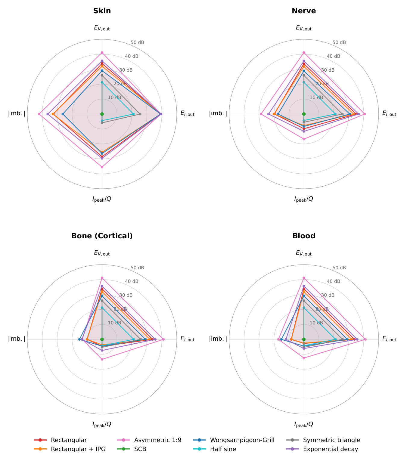
Table 6 lists the eight waveforms across the four benchmark axes. The three waveforms with the lowest (SCB, half sine, symmetric triangle) are also the three with the lowest on Skin, the lowest , and the lowest max |imbalance| across the panel. The remaining five waveforms cluster in a very different regime: on Skin above ninety-two per cent, above 47 nC−1, and max |imbalance| above one per cent. The distribution is bimodal on every axis, and the two groups are separated by at least an order of magnitude. The same partition reads at a glance on the radar synthesis of Figure 7, drawn on four representative tissues: the three lower-group waveforms collapse to a small polygon near the SCB reference at the centre of every panel, while the five upper-group waveforms form the large polygons that extend far along every axis. The reason is spelled out later in the discussion: the three lower-group waveforms meet zero at every phase boundary, whereas the five upper-group waveforms all carry at least one abrupt jump.
Table 6.
Synthesis of the campaign values across the four benchmark axes. Column keys: is the out-of-band voltage energy fraction averaged across the eight tissues; Skin is the out-of-band current energy fraction on Skin only; is the peak absolute current per unit delivered charge averaged across the eight tissues; imb. is the maximum absolute cyclic imbalance across the eight tissues after one hundred periods. Waveforms are ordered by , the primary spectral criterion.
| Waveform | (%) | Skin (%) | (μA/nC) | imb. (%) |
|---|---|---|---|---|
| SCB | 0.006 | 0.011 | 1.0 | 0.003 |
| Half sine | 0.77 | 1.44 | 2.7 | 0.0003 |
| Symmetric triangle | 2.24 | 4.01 | 3.5 | 0.0002 |
| Wongsarnpigoon–Grill | 4.54 | 92.80 | 57.9 | 1.17 |
| Rectangular + IPG | 9.00 | 95.50 | 47.7 | 5.39 |
| Rectangular | 13.76 | 97.34 | 92.4 | 5.08 |
| Exponential decay | 20.91 | 98.39 | 121.9 | 12.00 |
| Rectangular asym. 1:9 | 76.06 | 99.92 | 466.3 | 45.39 |
Figure 7.
Radar synthesis of the four benchmark axes on four representative tissues (Skin, Nerve, Bone (cortical), Blood). Each axis is normalised to the SCB of the same tissue and reported in decibels: radial distance from the centre equals , so the SCB sits at the centre and positive dB means “worse than SCB” on that axis. Rings mark 10, 20, 30, 40 and 50 dB. The three waveforms that survive the five-door funnel of Section 4.4 (SCB, half sine, symmetric triangle) collapse to small polygons near the centre; the five candidates that fail the funnel form the large polygons at the periphery of every panel. Waveform colours match Figure 1.
3.8. Reciprocity Across Drive Modes
The two campaigns (voltage-driven, current-driven) run at strictly matched delivered charge on each of the sixty-four tissue-waveform cells. For a linear passive network, the total port dissipation on the two campaigns is related to the driven waveform spectrum through
where is the port admittance and . Equal charge does not entail equal dissipation across modes: the imposed spectrum in the voltage-driven campaign is that of , weighted by ; the imposed spectrum in the current-driven campaign is that of , weighted by . The two integrals coincide only when is purely real over the significant band of the waveform.
Figure 8 plots the two campaign totals against each other, one point per tissue-waveform cell, on a base-ten logarithmic scale. Every point sits on or below the diagonal.
Figure 8.
Linear reciprocity across drive modes on the eight tissues by eight waveforms panel, at strictly matched delivered charge per cell. Horizontal axis: total port dissipation in the voltage-driven campaign, joules, log scale. Vertical axis: total port dissipation in the current-driven campaign, same units, same scale. Colours code the tissue. The dashed line marks the diagonal ; every point lies on or below it, showing that the current-driven mode delivers strictly less energy at equal charge.
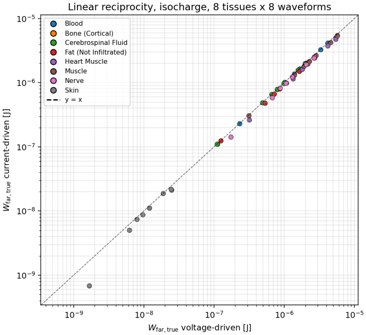
Empirically, on the eight-tissue panel and the eight waveforms, the current-driven campaign delivers strictly less dissipation than the voltage-driven campaign on every dispersive tissue. The mean deviation across the sixty-four cells is %, the maximum 83 %. On the resistive tissues (Blood, Cerebrospinal fluid, Bone (cortical)), for which Z is essentially real in the useful band, the deviation is below one per cent, in agreement with (1)–(2). On the dispersive tissues (Nerve, Heart muscle, Fat), the deviation scales with the high-frequency spectral content of the waveform, from about five per cent on the smooth waveforms to about twenty per cent on the exponential decay and on the asymmetric 1:9 rectangle. On Skin, whose polarisation network is capacitive over most of the useful band, the deviation reaches its worst case with the asymmetric 1:9 rectangle at 83 %.
The message for the design of an efficient stimulator is direct: at matched charge, a current-driven front end delivers strictly less energy to the tissue on every dispersive load, and the saving grows with the spectral asymmetry of the delivered waveform.
4. Discussion
The four axes of the benchmark converge on a single question: why should the stimulus carry frequency harmonics whose clinical benefit has not been established, and which the electrode-tissue interface literature identifies as sources of avoidable heat, interface stress, and long-term electrode wear [23,24,25,26]? The rectangle carries them because the silicon of the 1950s could deliver little else; the alternatives we tested carry fewer of them, and the tissue pays proportionally less for the same delivered charge.
Rather than discuss each axis in isolation, we walk through the four questions that a clinician facing a stimulation setup has to answer: why stimulate, what to stimulate, how to stimulate, and why the shape of the delivered signal matters. The four answers close, one by one, on a small set of candidate waveforms.
4.1. Why Stimulate?
Electrical stimulation is used clinically to recruit fibres that carry a signal the patient’s own physiology no longer carries adequately: motor axons after spinal injury or stroke, sensory afferents in chronic pain, retinal or cochlear afferents after receptor loss, autonomic pathways in refractory epilepsy or depression. In every case the target is a fibre population defined by anatomy and by the clinical problem. The stimulus has one job at that fibre: bring the membrane above the threshold for an action potential, then let the fibre do its own thing. Everything else the stimulus delivers to the tissue is a side effect. Two side effects are unavoidable in principle and dominate what a designer or a clinician has to worry about: heat and stress at the electrode-tissue interface, and recruitment of unintended fibres in the neighbourhood of the target. The waveform of the stimulus is the single knob that modulates both.
4.2. What to Stimulate?
An electric current that reaches a sodium channel has already crossed three physical layers. It has been shaped by the driver of the stimulator, filtered by the electrode-electrolyte interface, and transported through the tissue bulk between the electrode and the target fibre. Only at the fourth layer does it meet the biophysics of the axonal membrane. Each of the three upstream layers has its own transfer function, its own time constants, its own dissipation, and its own limits: the driver by its hardware, the interface by its electrochemistry, and the tissue by its Foster network. A waveform that the driver produces at the pin is not the waveform the fibre sees. The benchmark measures where in the chain the mismatch appears, and quantifies its magnitude on the tissue-side layer, at the terminals where the fibre lies.
4.3. How to Stimulate?
Taken together, the voltage and current spectra suggest a linear-system reading of the whole chain. At the terminals of the tissue, the voltage is (up to the fixed divider through the source resistance) the applied waveform. The tissue then transforms that voltage into a current whose spectral shape is set by the transfer function of the passive tissue network. The transfer function varies dramatically across the panel. Blood and Cerebrospinal fluid behave as pure resistors: the current follows the voltage instantaneously, and the leakage spectrum of the current matches that of the voltage. Skin behaves as a differentiator: the current is proportional to the derivative of the voltage, and a step in the voltage becomes an impulse in the current. Nerve, Bone, Muscle, Heart, and Fat interpolate between these two regimes, each with its own composition of resistive and reactive components.
The energy delivered by the stimulator ends up somewhere in this chain. Part of it dissipates through the tissue’s ionic conduction (the bulk conductive contribution). Part of it dissipates through the frequency-dependent polarisation of the water, membranes and macromolecules around the ionic paths (the dielectric contribution). The ratio of the two varies by four orders of magnitude across the eight tissues, from a Nerve-like regime dominated by dielectric losses to a Blood-like regime dominated by ionic conduction. This is a property of the tissues, not of the waveform: the ratio changes by less than a factor of two between the eight candidate waveforms on any given tissue.
The waveform matters more visibly on the hardware axis, where the peak current per unit delivered charge separates the eight candidates over nearly three decades: from about 1 nC−1 for the SCB to 466 nC−1 for the asymmetric 1:9 rectangle. That peak sets the driver transistor size, the compliance voltage, and the battery drain of the stimulator, on any tissue.
4.4. Why Waveform Shape Matters
The benchmark axes translate into five go/no-go questions that a stimulation waveform has to answer. Each question closes a door, and the doors close in a specific order.
Q1. Can a signal loaded with high-frequency harmonics do the job?
No. The fibre-level machinery has a characteristic time of about 500 (sodium activation), and anything above 2 is delivered energy that the fibre cannot use. It becomes heat inside the tissue and stress at the electrode-tissue interface. Out: rectangular biphasic, rectangular with interphase gap, exponential decay, rectangular asymmetric 1:9. All four carry at least one abrupt jump in value at a phase boundary, and push between 9 and 76 per cent of the voltage energy above the useful band.
Q2. Are we in a rush?
No. A phase duration of about 200 is already at the physiological limit; nothing forces the signal to compress the delivered charge into a spike shorter than that. Out: rectangular asymmetric 1:9, which crams the entire delivered charge into a 60 cathodic spike, ten times shorter than the useful time constant.
Q3. Do we accept the peak-current cost that a high-derivative signal forces on the driver hardware?
No, all else being equal. The peak current per unit charge sets the driver transistor size, the battery drain, and the compliance voltage. The plain rectangle demands nearly a hundred times the peak current of the SCB for the same clinical dose.
Q4. Do we accept a residual charge imbalance at long times?
No. A chronic stimulator has to converge to a strictly charge-balanced cycle for interface safety. Out: any candidate that fails the cyclic convergence test on the most capacitive tissue of the panel (Skin under a plain rectangle retains a five per cent imbalance after one hundred periods; the asymmetric 1:9 rectangle retains forty-five per cent).
Q5. Can the same charge be pushed through a miniaturised electrode without exceeding the safe injection window?
The field of implantable stimulation is moving toward smaller electrodes for better spatial selectivity. Safe charge-injection limits at the electrode-tissue interface are set in current density, not in absolute charge [23,24]. A rectangular waveform that pushes a 5 peak on a centimetre-scale electrode sits below those limits; the same waveform on a microelectrode a hundred times smaller crosses every published safety threshold, and the spatial precision that justified the miniaturisation is either lost to electrochemical damage or paid for with accelerated electrode corrosion. The SCB, with roughly a hundredth of the peak current for the same delivered charge, keeps the density inside the safe window at any electrode scale.
What Remains After the Five Questions
The SCB, the half sine, and the symmetric triangle: the three candidates that meet zero at every phase boundary. On every axis of the benchmark, these three cluster at least an order of magnitude below the five upper-group candidates (Table 6). The rectangle, in every variant, does not survive Q1. The industrial choice inherited from 1970s electronics has become a scientific outlier.
4.5. The Multilayer Case: TENS and Non-Invasive DBS
The single-tissue setting of the benchmark isolates each tissue’s electrical response for direct comparison, but does not match the clinical reality of transcutaneous nerve stimulation (TENS) or non-invasive deep brain stimulation, where the applied current crosses a stack of tissues in series (skin, fat, muscle or bone, target) before reaching the intended fibre.
The mechanics of the benchmark extend without conceptual change to that setting: each layer keeps its Foster admittance, the series constraint closes the system, and the current is shared by all layers. The waveform criterion of Section 4.4 is preserved and, if anything, amplified by the presence of a capacitive layer at the head of the stack: a skin layer acts as a differentiator on the current entering every layer behind it, and any waveform carrying an abrupt jump is filtered into a wideband current signature before it reaches the target.
A browser-based multilayer solver implementing this extension is under active development and will be made publicly available as a companion tool with the corresponding open dataset.
4.6. Scope and Prerequisites
The considerable computational literature on stimulation waveforms, from Hodgkin-Huxley through the MRG axon model of McIntyre et al. [27] to the modern NEURON-based studies of Foutz and McIntyre [7], Wongsarnpigoon and Grill [6], Hofmann et al. [8], Lempka et al. [2], and Ng et al. [10], has concentrated on the fourth layer, the axonal membrane. It has produced substantial insights into the biophysics of neural excitation and into the energy required to trigger an action potential in a given fibre geometry. The industrial rectangle emerged in that context, and the alternative shapes proposed as improvements were derived under the same methodological posture.
The present benchmark occupies a different position along that chain. It characterises the electrical signal actually delivered to the tissue, at its terminals, on a common eight-tissue panel and four quantitative axes. It does not model the axonal membrane, and it does not predict excitation thresholds, refractoriness or block conditions at the fibre level. It is a tissue-side benchmark, positioned as a prerequisite to any downstream fibre analysis rather than as a substitute for it.
The distinction matters because fibre-level pipelines routinely assume that the current injected into the model equals the nominal waveform prescribed at the stimulator. The present benchmark makes visible that this assumption does not hold in general. On the eight tissues of the panel, the effective spectral leakage of the current delivered at the tissue terminals varies by up to four orders of magnitude depending on the tissue and on the waveform, and the peak voltage response varies by several orders of magnitude at fixed nominal charge (Section 3.2 and Section 3.5). A fibre analysis that ignores this variability propagates a quantitatively different stimulus to every tissue it studies, without knowing so. The benchmark quantifies exactly what a rigorous fibre analysis must build upon.
The current-driven configuration of the benchmark (Section 2.4) makes the coupling explicit. The ideal current source Iin imposed on the tissue circuit in that mode matches the convention of NEURON’s IClamp point process [20,21], under which the stimulus is represented as an ideal current injection into the target compartment. A fibre model driven by IClamp therefore receives an input identical in kind to the input our current-driven benchmark measures at the tissue terminals. The two vantage points connect directly, and the benchmark output can serve as the input specification of a downstream fibre simulation.
Two consequences follow. A waveform that minimises the energy required to reach the excitation threshold at the fibre does not automatically minimise the spectral leakage or the peak tissue voltage in the surrounding tissue. A benchmark that quantifies the second does not replace a benchmark that quantifies the first. A complete design study of a stimulation waveform benefits from both, and the present work provides one of the two.
4.7. Limitations
Seven simplifications of the benchmark deserve explicit mention.
We model the tissue as a purely passive Foster network with a DC ionic branch and four Cole–Cole dispersions. We do not model the electrode-electrolyte interface, which behaves electrically as an additional capacitive layer at the electrode surface (the Randles-cell equivalent circuit of the electrochemistry literature). Adding this interface term shifts the tissue-side ordering of the spectral leakage of the current, but does not affect the tissue-independent ordering of the spectral leakage of the voltage, which is our central result.
The benchmark comes in two operating modes, both of which are simplifications. The voltage-driven campaign uses a single 50 output impedance to model a real stimulator; the current-driven campaign uses an ideal current source, following the NEURON IClamp convention [20,21], and is therefore independent of output impedance by construction. Neither choice captures the full envelope of stimulator front ends found in practice, and a design study using this benchmark should re-evaluate the axes at its own output impedance; our pipeline supports both. We also use a single reference geometry, a slab of 1 cm2 by 1 , which fixes the absolute values of the resistances and capacitances of the equivalent circuits, and therefore the absolute values of the currents and energies; the relative ordering of the waveforms is invariant to the geometry.
The reciprocity result of Section 3.8, namely that the current-driven mode delivers strictly less dissipation than the voltage-driven mode at matched charge, rests on the linearity and passivity of the Foster tissue model. Any nonlinear response of the tissue would break both the linearity assumption and the inequality; in particular, at voltages high enough to open transient pores in the cell membrane (the electroporation regime), the tissue no longer behaves as a passive Foster network, and the reciprocity ordering no longer applies. The reported ordering therefore holds only in the sub-threshold linear regime of tissue polarisation.
The delivered power that does not become an excitation signal does not vanish. Its fate on time scales longer than the stimulation period is the concern of a large literature on electrode-tissue interfaces [23,24,25,26], and the tissue-dependent dispersion patterns reported here define the input to that concern.
We do not include a nerve fibre model. A rigorous prediction of excitation thresholds requires coupling our tissue benchmark to a computational fibre model, in the spirit of the studies cited above. Our benchmark focuses on the tissue-side quantities that condition any downstream fibre model, and treats the fibre-side predictions as a separate concern.
The energy decomposition of Section 2.5 and Appendix D is defined branch by branch on the specific Foster synthesis used here (twelve Debye branches per Cole–Cole dispersion, joint fit of time constants and weights, see Section 2.2). A different synthesis (fewer branches, a different fit algorithm, or a canonical Foster I form in place of the Foster II form we use) would produce numerically different per-branch dissipations, but the same total up to the fit residual, and the same ratio in each regime. Which regime a given tissue-waveform pair falls into is therefore a property of the tissue and the waveform, not of the synthesis.
Finally, the Foster synthesis reaches its two per cent target residual on most of the twenty-six dispersions of the panel but not all. Six dispersions carry a larger max residual over the check range, of which four are above three per cent: Bone (cortical) dispersion 3 at 17 %, Muscle dispersion 3 at 13 %, Heart muscle dispersion 3 at 8.5 %, and Fat (not infiltrated) dispersion 3 at 4.6 %. The two remaining, Fat dispersions 2 and 4, sit at 2.4 and 2.7 % respectively. All six residuals sit at frequencies where the tissue admittance is dominated by other branches, and we verified on the sixty-four cells that they do not shift any reported spectral or energetic metric by more than 0.1 %.
5. Conclusions
We built a comparison benchmark for stimulation waveforms across eight target tissues, on four independent quantitative axes: spectral leakage of the terminal voltage, spectral leakage of the delivered current, bulk conductive and dielectric shares of the energy budget, and peak current per unit delivered charge. A fifth check, cyclic convergence, verifies that each combination settles into a well-defined steady-state cycle.
Across all four axes and all eight tissues, an SCB waveform dominates the other seven candidates. The industrial rectangle sits at the opposite end of the ordering, with a peak current requirement about ninety times higher and a spectral leakage about two thousand times higher than the SCB, at fixed clinical dose. Its clinical asymmetric 1:9 variant sits even further out on every metric. The five other alternatives (the rectangle with interphase gap, the half sine, the symmetric triangle, the Wongsarnpigoon-Grill truncated Gaussian, and the exponential decay) take intermediate positions that shift with the axis and with the tissue but never overturn the ranking of the endpoints.
The benchmark is portable and reproducible. Any waveform can be dropped into the pipeline for direct comparison, and any tissue for which four-dispersion Cole–Cole parameters exist can be added to the panel. The ngspice decks, the Foster subcircuits, and the analysis scripts are provided as supplementary material.
Author Contributions
Bernard Delalande: Conceptualization, Methodology, Software, Formal analysis, Investigation, Data curation, Visualization, Writing (original draft), Writing (review and editing). Hirohisa Tamagawa: Conceptualization, Supervision, Validation, Writing (review and editing). Both authors read and approved the final manuscript.
Funding
No funding was received for conducting this study.
Informed Consent Statement
Not applicable. This study did not involve human participants or animal subjects. All data derive from numerical simulations based on published dielectric parameters (IT’IS Foundation database V5.0 and Gabriel et al. [13]).
Data Availability Statement
The simulation datasets generated and analysed during the current study, including the campaign master file (64 runs, eight waveforms across eight tissues), the Python pipeline (waveform library, campaign runner, Foster synthesis), and the ngspice deck templates, are deposited on Zenodo. DOI: https://doi.org/10.5281/zenodo.21376086.
Use of Artificial Intelligence
The authors used Anthropic’s Claude as a working assistant during manuscript preparation. Specific uses were: language editing of the English text, cross-checking of LaTeX consistency, cross-checking of bibliographic references, and assistance with the Python figure-generation pipeline. All simulation code, ngspice deck implementations, scientific claims, analyses, and interpretations remain the sole responsibility of the authors, who verified every quantitative result independently. No AI tool contributed to the design of the study, to the choice of the eight-tissue testbed, or to the design of the eight waveforms.
Conflicts of Interest
The authors declare that they have no competing interests, financial or non-financial, that could have appeared to influence the work reported in this paper.
Appendix A. The Cole–Cole Model and the Foster Synthesis
The dielectric behaviour of each tissue is captured by a four-dispersion Cole–Cole model. The complex relative permittivity of the tissue reads
where each of the four dispersions k is described by a permittivity increment , a relaxation time and a broadening exponent . The additional parameters are the high-frequency permittivity and the DC ionic conductivity , giving fourteen parameters per tissue. The parameter values are those tabulated in version 5.0 of the IT’IS Foundation database, itself a curated extension of Gabriel et al. [13].
The Foster synthesis represents Equation (A1) as an equivalent lumped-element circuit whose admittance approximates the target permittivity in the frequency range of interest. The chosen construction is a Foster-II network in admittance form:
where each Cole–Cole dispersion is approximated by a sum of Debye sub-branches with pole-residue pairs . The DC branch is , with A and d the reference cross-section and thickness of the tissue slab. The high-frequency capacitor is .
Figure A1.
Internal structure of the tissue Foster subcircuit that appears as a generic two-terminal block in Figure 2. Six branches sit in parallel between node a and ground: the high-frequency capacitor , the DC ionic conductance , and one block per Cole–Cole dispersion. Each block expands into Debye sub-branches, one of which is detailed in the zoom.
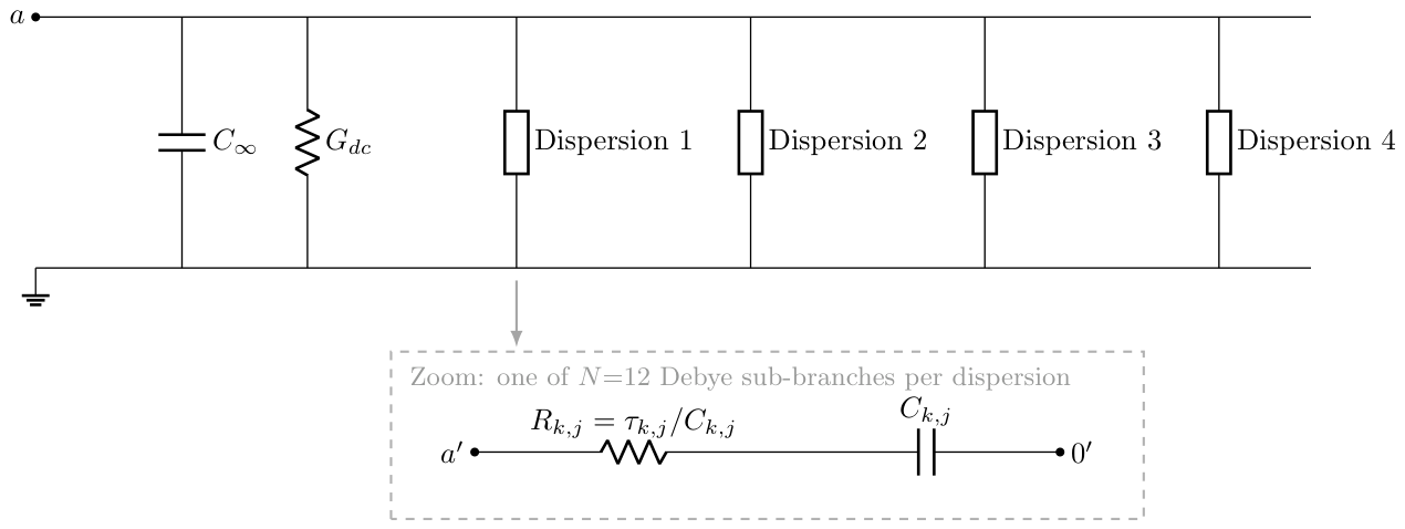
The pole-residue pairs are fitted by joint non-linear least squares in the domain, from 1 to 100 . The cost function equally weights the relative error on and on . The twelve pairs of a given dispersion are fitted jointly, but the four dispersions are fitted independently because they are additive. Across the eight tissues and the twenty-six non-degenerate dispersions of the panel, twenty-five fits converged below two per cent relative error in . The one exception is the fourth dispersion of Fat (not infiltrated), at 3.25 per cent.
The synthesised networks are emitted as ngspice subcircuit files, one file per tissue, with a two-terminal interface.
Appendix B. The Slope-Continuous Biphasic (SCB) Waveform
The SCB waveform is composed of three concatenated cubic Bézier segments. The first segment rises from to , the second descends from to , and the third returns from to . For the reference parameter set adopted throughout this paper we use , , , and .
A cubic Bézier segment is parametrised by four control points and reads
For each of our three segments, the two internal control points and are chosen with the y-coordinate of their nearest endpoint: shares the y-coordinate of , and shares the y-coordinate of . This choice forces at both and for every segment. The x-coordinates of the two internal control points are placed at and , respectively, where T is the duration of the segment and is a shape parameter that controls the sharpness of the segment. Concatenating the three segments produces a curve of class : value and slope are continuous at every junction. This is the property the name SCB records. The default shape parameter is .
The hyperpolarisation amplitude is calibrated numerically to enforce a strictly zero net charge over the active phase . The calibration uses Brent’s method on a fine-sampled integral of the parametric curves. For and the reference V, , , above, the result is .
The SCB waveform described in this appendix is released by the authors for unrestricted use. Anyone is free to implement it in research protocols, medical devices, or commercial products, without royalty, licence fee, or attribution requirement beyond scientific citation of this paper.
Appendix C. ngspice Deck Implementation
Each simulation is defined by an ngspice deck of the form
.include tissue_<name>.sp
.include waveform_<name>_long.inc
Rsrc in a 50
X1 a 0 tissue_<name>
.tran <dt_max> <t_end> <t_start> <dt_max>
.control
set filetype=ascii
set wr_singlescale
run
wrdata results.dat V(a) i(vin)
quit
.endc
.end
The tissue subcircuit is included from a file generated by the Foster synthesis of Appendix A. The waveform is included from a separate file that expands the samples of one period, concatenated over periods, into an inline piecewise-linear voltage source Vin. This detour through an include file is necessary because the syntax PWL FILE=<file>, quoted in various third-party tutorials, is not implemented in ngspice, as confirmed by the maintainer H. Vogt on the developer mailing list. The chained samples typical file is around per waveform, compressed adaptively to keep sharp transitions of the rectangular pulse at the original 200 resolution while thinning slowly varying regions.
The transient runs from to with a maximum time step . The optional argument restricts the wrdata output to the last period, which reduces the disk footprint by a factor of about a hundred.
The current through the voltage source is reported by ngspice with the internal convention where positive current flows from the positive terminal to the negative terminal inside the source. For a source driving an external load, this convention gives a current with a sign opposite to the physical current entering the tissue. The post-processing script therefore flips the sign of the current channel on read.
Appendix D. Formal Definitions of the Metrics
The four axes described qualitatively in Section 2.5 correspond to the following definitions. Let and denote the voltage at the tissue terminals and the physical current entering the tissue, on the last period .
Per-Phase Charge
The positive-phase charge is
the negative-phase charge is
and the residual imbalance in per cent of the largest per-phase charge is
A strictly steady-state cycle satisfies . We take as the operational acceptance threshold.
Energy Budget
The total energy delivered on the period is
where is the terminal voltage and is the physical current entering the tissue. The Foster network of Section 2.2 has three kinds of parallel branches at the tissue port, characterised by their admittance: for the DC ionic path, for the high-frequency permittivity, and for each of the N Debye branches synthesised from the four Cole–Cole dispersions. Only the resistors dissipate. The bulk conductive dissipation is the loss in the DC ionic branch,
and the dielectric dissipation is the sum of the losses in the N Debye resistors,
where the branch current is the solution, under the periodic boundary condition , of the first-order linear ordinary differential equation
The identity that ties the two dissipation terms to the port energy is
where the residual vanishes for a strictly periodic response and is bounded in practice by the cyclic convergence acceptance threshold of Section 3.6. Equations (A8)–(A10) are valid in both voltage-driven and current-driven modes, since they depend on the recorded and on the Foster parameters alone. The regime is labelled by the ratio : values above 100 identify a bulk-dominated dissipation, values below unity a dielectric-dominated dissipation, and intermediate values a mixed regime. For tissues in which the Cole–Cole dispersions carry essentially no weight ( below the resolution of the transient solver), the ratio saturates and the run is flagged as conductive-pure.
The branch currents are computed spectrally from the recorded : the discrete Fourier transform is multiplied by the branch admittance , and is recovered by inverse transform. This route is exact for a periodic , has cost per branch, and does not require solving the transient a second time; it applies equally to the voltage-driven and current-driven campaigns.
Peak Current per Unit Charge
The peak absolute current on the last period is , and the hardware demand metric is
expressed in milliamperes per nanocoulomb.
Spectral Band Split
The discrete Fourier transforms and are computed on a uniform resample of the last-period signals, with samples over one period. The useful band is with . The fraction of voltage energy leaking outside the useful band is
and is defined analogously on .
References
- Butson, C.R.; McIntyre, C.C. Differences among implanted pulse generator waveforms cause variations in the neural response to deep brain stimulation. Clin. Neurophysiol. 2007, 118, 1889–1894. [Google Scholar] [CrossRef] [PubMed]
- Lempka, S.F.; Howell, B.; Gunalan, K.; Machado, A.G.; McIntyre, C.C. Characterization of the stimulus waveforms generated by implantable pulse generators for deep brain stimulation. Clin. Neurophysiol. 2018, 129, 731–742. [Google Scholar] [CrossRef] [PubMed]
- Furman, S.; Schwedel, J.B. An intracardiac pacemaker for Stokes-Adams seizures. N. Engl. J. Med. 1959, 261, 943–948. [Google Scholar] [CrossRef] [PubMed]
- Wilson, B.S.; Finley, C.C.; Lawson, D.T.; Wolford, R.D.; Eddington, D.K.; Rabinowitz, W.M. Better speech recognition with cochlear implants. Nature 1991, 352, 236–238. [Google Scholar] [CrossRef] [PubMed]
- Sluka, K.A.; Walsh, D. Transcutaneous electrical nerve stimulation: basic science mechanisms and clinical effectiveness. J. Pain 2003, 4, 109–121. [Google Scholar] [CrossRef] [PubMed]
- Wongsarnpigoon, A.; Grill, W.M. Energy-efficient waveform shapes for neural stimulation revealed with a genetic algorithm. J. Neural Eng. 2010, 7, 046009. [Google Scholar] [CrossRef] [PubMed]
- Foutz, T.J.; McIntyre, C.C. Evaluation of novel stimulus waveforms for deep brain stimulation. J. Neural Eng. 2010, 7, 066008. [Google Scholar] [CrossRef] [PubMed]
- Hofmann, L.; Ebert, M.; Tass, P.A.; Hauptmann, C. Modified pulse shapes for effective neural stimulation. Front. Neuroeng. 2011, 4, 9. [Google Scholar] [CrossRef] [PubMed]
- Delalande, B. Étude scientifique comparative pour la validation d’un courant de neurostimulation: courant rectangulaire à moyenne nulle. Ann. Kinésithér. 2000, 28, 88–96. [Google Scholar]
- Ng, P.R.; Bush, A.; Vissani, M.; McIntyre, C.C.; Richardson, R.M. Biophysical principles and computational modeling of deep brain stimulation. Neuromodulation Technol. At. Neural Interface 2024, 27, 422–439. [Google Scholar] [CrossRef] [PubMed]
- Gilbert, Z.D.; Mason, X.; Sebastian, R.; Tang, A.M.; Del Campo-Vera, R.M.; Chen, K.H.; Leonor, A.; Paulo, D.L.; Tabarestani, T.Q.; Barbaro, M.F.; et al. A review of neurophysiological effects and efficiency of waveform parameters in deep brain stimulation. Clin. Neurophysiol. 2023, 152, 93–111. [Google Scholar] [CrossRef] [PubMed]
- Lucarelli, D.; Guidali, G.; Guidotti, R.; Pieramico, G.; Bolognini, N.; Romani, G.L.; Pizzella, V.; Marzetti, L. Pulse waveform and current direction alter network-level TMS-induced functional connectivity: evidence from TMS-EEG. NeuroImage 2026, 328, 121794. [Google Scholar] [CrossRef] [PubMed]
- Gabriel, S.; Lau, R.W.; Gabriel, C. The dielectric properties of biological tissues: III. Parametric models for the dielectric spectrum of tissues. Phys. Med. Biol. 1996, 41, 2271–2293. [Google Scholar] [CrossRef] [PubMed]
- Lembcke, L.; Bathel, H.; Zimmermann, J.; Engel, V.; Bader, R.; Frerich, B.; van Rienen, U.; Springer, A.; Engel, N.; Kämmerer, P.W. A validated in vitro approach for low-frequency alternating-current stimulation of stem cells: from electrode characterization to biological responses. Protoplasma 2026, pp. 1–24. published online 18 April 2026. 2026. [CrossRef] [PubMed]
- Hasgall, P.A.; Di Gennaro, F.; Baumgartner, C.; Neufeld, E.; Lloyd, B.; Gosselin, M.C.; Payne, D.; Klingenböck, A.; Kuster, N. IT’IS Database for thermal and electromagnetic parameters of biological tissues, Version 5.0, 2022. year to be confirmed against IT’IS Foundation release notes. [CrossRef]
- Gabriel, C.; Gabriel, S.; Corthout, E. The dielectric properties of biological tissues: I. Literature survey. Phys. Med. Biol. 1996, 41, 2231–2249. [Google Scholar] [CrossRef] [PubMed]
- Gabriel, S.; Lau, R.W.; Gabriel, C. The dielectric properties of biological tissues: II. Measurements in the frequency range 10 Hz to 20 GHz. Phys. Med. Biol. 1996, 41, 2251–2269. [Google Scholar] [CrossRef] [PubMed]
- Andreuccetti, D.; Fossi, R.; Petrucci, C. An Internet resource for the calculation of the dielectric properties of body tissues in the frequency range 10 Hz to 100 GHz. 1997. [Google Scholar]
- Lilly, J.C.; Hughes, J.R.; Alvord, E.C.J.; Galkin, T.W. Brief, Noninjurious Electric Waveform for Stimulation of the Brain. Science 1955, 121, 468–469. [Google Scholar] [CrossRef] [PubMed]
- Hines, M.L.; Carnevale, N.T. The NEURON simulation environment. Neural Comput. 1997, 9, 1179–1209. [Google Scholar] [CrossRef] [PubMed]
- Carnevale, N.T.; Hines, M.L. The NEURON Book; Cambridge University Press, 2006. [Google Scholar] [CrossRef]
- ngspice development team. ngspice open source mixed-mode circuit simulator, users manual, version 46. 2024.
- Merrill, D.R.; Bikson, M.; Jefferys, J.G.R. Electrical stimulation of excitable tissue: design of efficacious and safe protocols. J. Neurosci. Methods 2005, 141, 171–198. [Google Scholar] [CrossRef] [PubMed]
- Cogan, S.F. Neural stimulation and recording electrodes. Annu. Rev. Biomed. Eng. 2008, 10, 275–309. [Google Scholar] [CrossRef] [PubMed]
- Cantrell, D.R.; Inayat, S.; Taflove, A.; Ruoff, R.S.; Troy, J.B. Incorporation of the electrode-electrolyte interface into finite-element models of metal microelectrodes. J. Neural Eng. 2008, 5, 54–67. [Google Scholar] [CrossRef] [PubMed]
- Boehler, C.; Carli, S.; Fadiga, L.; Stieglitz, T.; Asplund, M. Tutorial: guidelines for standardized performance tests for electrodes intended for neural interfaces and bioelectronics. Nat. Protoc. 2020, 15, 3557–3578. [Google Scholar] [CrossRef] [PubMed]
- McIntyre, C.C.; Richardson, A.G.; Grill, W.M. Modeling the excitability of mammalian nerve fibers: influence of afterpotentials on the recovery cycle. J. Neurophysiol. 2002, 87, 995–1006. [Google Scholar] [CrossRef] [PubMed]
Disclaimer/Publisher’s Note: The statements, opinions and data contained in all publications are solely those of the individual author(s) and contributor(s) and not of MDPI and/or the editor(s). MDPI and/or the editor(s) disclaim responsibility for any injury to people or property resulting from any ideas, methods, instructions or products referred to in the content. |
© 2026 by the authors. Licensee MDPI, Basel, Switzerland. This article is an open access article distributed under the terms and conditions of the Creative Commons Attribution (CC BY) license (http://creativecommons.org/licenses/by/4.0/).
Copyright: This open access article is published under a Creative Commons CC BY 4.0 license, which permit the free download, distribution, and reuse, provided that the author and preprint are cited in any reuse.