

Submitted:
02 October 2026
Posted:
05 October 2026
You are already at the latest version
Abstract
Reliable ginseng authentication requires analytical signatures that distinguish plant category, production region, and growth duration while remaining interpretable and operationally compact. This study evaluated laser-induced breakdown spectroscopy (LIBS) as a proximal elemental-sensing method for these three classification tasks. The datasets comprised 200 spectra from four plant categories, 100 spectra from two geographical origins, and 100 spectra from two growth years; each class contained 50 pressed pellets prepared from one homogenized powder batch. Four chemometric pipelines were compared using five-fold nested cross-validation repeated five times, with all preprocessing and model selection confined to training folds. The best mean balanced accuracies were 1.000, 0.982, and 1.000 for plant category, origin, and growth year, respectively. A sparse model using only 50 of 12,990 wavelengths retained balanced accuracies of 1.000, 0.980, and 1.000. Stable regions were provisionally associated with Ba, Sr, and K for plant category, Al for origin, and Ca and Fe for growth year. Standard normal variate preprocessing suppressed sensitivity to uniform intensity scaling and offsets, whereas detector-channel shifts caused marked deterioration. The results show that compact LIBS fingerprints can encode multiple ginseng attributes and identify wavelength registration, rather than intensity variation alone, as a central requirement for future transfer across batches and measurement settings.
Keywords:
ginseng authentication
; laser-induced breakdown spectroscopy
; proximal sensing
; support vector machine
; nested cross-validation
; wavelength selection
; elemental fingerprint
; medicinal plants
1. Introduction
Ginseng is a high-value medicinal plant for which botanical identity, geographical origin, and growth duration influence quality assessment, commercial grading, and traceability. Processing into slices or powders weakens visible diagnostic traits, while conventional chromatographic and molecular assays can require extensive preparation, reagents, or targeted prior knowledge. Spectral methods offer a complementary route because they can capture chemical variation rapidly and couple it with multivariate classification. In ginseng, LIBS and hyperspectral imaging have already been used to distinguish plant categories, regions, and ages [1], and recent studies have extended this direction through LIBS-hyperspectral fusion [2], near-infrared-LIBS fusion [3], and LIBS-Raman fusion [4]. Collectively, these studies show that elemental and molecular spectra contain useful provenance information, but they also raise the practical question of how much discrimination can be retained with a compact LIBS fingerprint.
Laser-induced breakdown spectroscopy (LIBS) focuses a pulsed laser onto the sample surface, forms a transient plasma, and records element-dependent atomic and ionic emission. The technique provides rapid multielement measurement with limited chemical preparation and has been applied to food authentication and quality assessment [5]. Reviews of plant materials describe direct analysis of leaves, roots, fruits, wood, and pressed plant powders [6], while broader agricultural reviews cover nutrient diagnosis, soil and crop monitoring, contaminants, and product classification [7,8,9,10,11]. These studies consistently identify matrix effects, ablation variability, spectral redundancy, and calibration transfer as barriers between high laboratory accuracy and dependable analytical deployment.
Medicinal plants are a particularly relevant application because species substitution, origin mislabeling, and compositional heterogeneity can alter both value and use. LIBS combined with chemometrics has differentiated medicinal plant tissues and elemental profiles [12], and PCA-neural-network models have classified Chinese herbal medicines by material type, origin, or plant part [13]. Plant-leaf classification using selected LIBS lines has further shown that compact elemental variables can retain high discrimination [14]. Elemental fingerprints have also supported geographical classification of tea [15], while combined LIBS and hyperspectral data have been used to trace rice origin [16]. These examples place ginseng within a broader movement toward rapid proximal spectroscopy for plant-resource authentication.
Recent agricultural and food spectroscopy has increasingly paired high-dimensional measurements with machine learning. The seven studies supplied with this project illustrate complementary aspects of that development. A deep spectral autoencoder was used for non-targeted hyperspectral screening of Fritillaria adulterants [17], and hyperspectral models were developed for sodium saccharin quantification in cat food powder [18], nested-cross-validated provenance classification of Curcumae Radix [19], and sulfite analysis in goji berry powder [20]. A controlled bean-seed benchmark published in the target Plants Special Issue similarly compared machine- and deep-learning strategies across visible, near-infrared, and shortwave-infrared spectra [21]. Although these studies use different matrices and spectral mechanisms, they demonstrate the importance of preprocessing, validation design, feature representation, and explicit robustness testing in agricultural spectroscopy.
The same methodological issues are prominent in LIBS. Discriminative restricted Boltzmann machines have been proposed for classification under high-dimensional, small-sample conditions [22]; uncertainty-aware neural networks have been used for small-sample LIBS quantification [23]; and self-supervised blind-spot denoising with Kolmogorov-Arnold networks has addressed spectral noise and nonlinear calibration [24]. Such models can extract complex structure, but higher model complexity does not remove the need for leakage-free validation or stable chemical interpretation. For datasets with many wavelength channels and comparatively few biological materials, the reliability of the validation hierarchy is at least as important as nominal model flexibility.
A further issue is whether a model depends on broad intensity patterns or on reproducible elemental regions. Full-spectrum models may average information across many channels but can also absorb redundant or instrument-specific variation. Sparse models reduce dimensionality and can reveal candidate emission lines, yet they may become sensitive to wavelength registration when individual detector channels are used. Comparing these two regimes under controlled perturbations can therefore distinguish resistance to intensity variation from resistance to spectral displacement, two properties that are often combined under the general label of robustness.
This study developed an interpretable LIBS framework for classifying ginseng by plant category, geographical origin, and growth year. Four complementary classifiers were evaluated using repeated nested cross-validation. The analysis then examined feature-selection stability, performance across wavelength budgets, and sensitivity to simulated noise, intensity changes, and detector-channel shifts. The aim was to determine how much predictive information could be compressed into a stable elemental fingerprint and to identify the experimental and computational conditions that would govern its future use in plant-material screening.
2. Results
2.1. Spectral Patterns and Exploratory Structure
The mean spectra shared a common mineral-emission background but showed task-dependent differences in peak intensity (Figure 1). The strongest between-class contrasts were concentrated in narrow wavelength regions rather than appearing as uniform displacement of the full spectrum. This pattern supports evaluating both global multivariate models and targeted wavelength-selection strategies.
Across the three datasets, the main emission structures occurred at comparable wavelengths, as expected for plant powders containing a shared set of major and trace elements. Class differences were expressed primarily as changes in relative peak magnitude and in groups of neighboring channels. The plant-category spectra showed the broadest set of visible deviations, whereas the two origin means were more similar over much of the range and diverged at selected peaks. The two growth-year classes showed repeated intensity differences in several visible and near-infrared regions. Because the spectra are plotted after logarithmic transformation, the figure emphasizes the coexistence of intense and weaker lines; it does not convert emission intensity into elemental concentration.
The first two principal components explained 55.1% of the variance for plant category, 79.9% for geographical origin, and 82.4% for growth year (Figure 2). Separation in the displayed score space was strongest for growth year and geographical origin. The four plant categories showed clear structure but greater overlap in two dimensions, indicating that additional components were useful for supervised classification.
For plant category, the Korean and American groups occupied largely different regions of the PC1-PC2 plane, while the Chinese and Japanese groups were closer and showed partial overlap. This structure explains why the first two components provided useful visualization without fully representing the decision space used by the supervised models. In the origin dataset, the Changbai Mountains group was concentrated mainly toward negative PC1 scores, whereas the Changchun group extended across a wider score range. The growth-year classes were separated principally along PC1, with only limited contact between their covariance ellipses. Thus, the exploratory analysis suggested that growth year was the most strongly expressed low-dimensional contrast, while plant category required information beyond the first two components.
2.2. Classification Performance
All four pipelines classified the controlled spectra accurately (Table 1; Figure 3). Plant-category balanced accuracy ranged from 0.993 to 1.000, whereas growth-year balanced accuracy ranged from 0.994 to 1.000. Geographical origin was the most difficult attribute, with balanced accuracy ranging from 0.968 for PLS-DA to 0.982 for the sparse SVM. The limited difference between full-spectrum and sparse models indicated substantial redundancy among the 12,990 wavelength variables.
For plant category, the full-spectrum linear SVM achieved 1.000 balanced accuracy in every outer fold. PLS-DA, PCA-RBF-SVM, and the sparse SVM also exceeded 0.99 on average, with standard deviations of 0.010, 0.014, and 0.005, respectively. The agreement between balanced accuracy, macro-F1, and MCC shows that performance was not driven by one category at the expense of the others. The sparse model's low fold-to-fold variation further indicates that most outer training subsets recovered a similar discriminative signal despite using only 50 wavelengths.
Origin classification showed a different pattern. The best mean balanced accuracy was 0.982 for the sparse SVM, followed by 0.980 for both the full-spectrum linear SVM and PCA-RBF-SVM; PLS-DA reached 0.968. Standard deviations of 0.024-0.032 were also larger than those observed for the other tasks. These results identify origin as the limiting classification problem in the present experiment and suggest that its spectral contrast was both weaker and more dependent on the exact composition of the training fold. For growth year, the full-spectrum and sparse linear SVMs both achieved 1.000, while the two latent-variable approaches remained close to unity but showed occasional fold-level errors.
2.3. Spectral Compression
Ten wavelengths were sufficient to obtain balanced accuracies of 0.989, 0.968, and 1.000 for plant category, geographical origin, and growth year, respectively (Table 2; Figure 4). Fifty wavelengths provided a favorable common operating point, yielding 1.000, 0.980, and 1.000 for the three tasks. Adding more variables did not consistently improve origin classification, consistent with a limited number of informative regions embedded in a high-dimensional spectrum.
The compression trajectories differed by task (Figure 4). Plant-category performance increased from 0.989 with 10 wavelengths to 1.000 with 50 and 100 wavelengths, then changed only slightly at 200 wavelengths. Growth-year performance remained at 1.000 throughout the tested range, showing that its discriminative structure was concentrated in very few channels. Origin accuracy improved from 0.968 at 10 wavelengths to 0.980 at 50 wavelengths, but decreased to 0.970 and 0.964 when 100 and 200 wavelengths were retained. The larger origin error bars indicate that its optimum was less stable across folds than the flat growth-year response.
The absence of monotonic improvement with additional wavelengths is analytically important. If the result were controlled mainly by accumulated signal, performance would be expected to increase or plateau as more channels were added. Instead, origin classification deteriorated after 50 variables, consistent with the addition of redundant or fold-specific variation. Fifty wavelengths were therefore retained as a common compromise: the setting captured the plant-category and growth-year maxima and remained near the origin optimum while reducing the input dimension by 99.62%.
2.4. Stable Wavelengths and Candidate Elemental Interpretation
The sparse models repeatedly selected compact spectral regions that differed among tasks (Table 3; Figure 5). Candidate Ba II, Sr I, and K I lines occurred among stable plant-category variables. Candidate Al I lines near 308.215, 309.283, and 396.152 nm were associated with geographical origin, while candidate Ca I and Fe I lines occurred among stable growth-year variables. Several highly stable wavelengths remained unassigned, particularly between 430 and 490 nm and near 648–651 nm. Because spectral overlap and matrix effects are possible, these assignments require confirmation using reference materials and detailed line-shape inspection before mechanistic interpretation.
Selection frequency distinguished isolated findings from features repeatedly recovered during resampling. For plant category, candidate Ba II lines near 455.402 and 493.407 nm were selected in all outer folds, the candidate Sr I line near 431.904 nm appeared in 96%, and the candidate K I line near 404.414 nm appeared in 80%. For origin, candidate Al I features near 308.215 and 309.283 nm were selected in every fold and the 396.152 nm feature appeared in 96%. For growth year, candidate Ca I features near 422.672 and 854.209 nm and the candidate Fe I feature near 866.371 nm were recovered in all outer folds. These high frequencies support reproducibility of the selected regions within the current resampling structure.
The unassigned channels are equally informative for interpreting the model. Several clusters contained multiple adjacent detector positions with high selection frequency, which is consistent with a broadened emission feature, a blend of lines, or correlated local background rather than independent chemical markers at every channel. The selected variables should therefore be treated as wavelength neighborhoods. Future confirmatory work should examine local peak shapes, replicate standards, and reference spectra before assigning individual elements or attributing the observed class separation to concentration differences.
2.5. Sensitivity to Spectral Perturbations
Gaussian noise up to 5% had limited influence on the full-spectrum model and caused only modest task-dependent changes in the sparse model (Figure 6). Under 20% multiplicative scaling, full-spectrum balanced accuracy decreased to 0.81 for plant category, 0.91 for origin, and 0.82 for growth year, whereas the SNV-based sparse model retained 1.00, 0.98, and 1.00. Similar protection was observed for additive offsets. In contrast, detector-channel shifts substantially degraded some sparse models. A negative shift of two indices reduced plant-category balanced accuracy to 0.255, while a positive shift of two indices reduced origin and year performance to 0.67 and 0.62. Wavelength registration was therefore identified as a critical transfer variable.
The heat map separates three kinds of sensitivity. First, random noise produced comparatively small losses: at 5% noise, the sparse model retained balanced accuracies of 0.95, 0.95, and 1.00 for plant category, origin, and growth year, respectively. Second, uniform intensity changes affected the unnormalized full-spectrum SVM much more strongly than the SNV-based pipeline. A 5% additive offset reduced full-spectrum performance to 0.92, 0.96, and 0.96, while the sparse model remained at 1.00, 0.98, and 1.00. The scale test produced the same contrast, indicating that per-spectrum centering and scaling removed much of this nuisance variation.
Third, wavelength displacement produced asymmetric, task-specific failures that neither model fully avoided. For plant category, shifting by -2 channels reduced balanced accuracy to 0.43 for the full-spectrum model and 0.26 for the sparse model. For origin, +2 channels reduced the corresponding values to 0.51 and 0.67. Growth-year performance was comparatively stable for the full-spectrum model but fell to 0.62 for the sparse model at +2 channels. The asymmetry reflects the local shape and neighborhood of the discriminative regions: moving a feature toward a nearby correlated channel is less damaging than moving it away from the informative peak. This result directly motivates wavelength calibration checks and window-based features in subsequent measurements.
3. Discussion
The principal finding is that three commercially relevant ginseng attributes were encoded in reproducible LIBS patterns under the controlled conditions of this experiment. Plant category and growth year were nearly or completely separable across all modeling strategies, whereas geographical origin produced lower means and larger fold-to-fold variation. This hierarchy agrees with the exploratory PCA structure and suggests that origin-related differences are subtler than the contrasts associated with plant category or growth duration. Earlier ginseng studies reported strong discrimination using LIBS together with hyperspectral, near-infrared, or Raman information [1-4]. The present results show that the LIBS component itself contains sufficient elemental contrast for these tasks in the measured materials, while also identifying where the classification margin is narrowest.
The strong performance of the linear SVM is informative because greater model complexity did not provide a consistent advantage. For plant category and growth year, a linear boundary matched or exceeded PCA-RBF-SVM and PLS-DA. Origin classification benefited modestly from SNV and variable selection, but not from the nonlinear PCA-RBF pipeline. This pattern indicates that the dominant discriminatory information was distributed in a form that became approximately linear after scaling or per-spectrum normalization. It also supports a parsimonious modeling strategy: when a simple classifier performs as well as a nonlinear alternative under the same nested validation, the simpler model offers clearer coefficients, lower computational cost, and fewer opportunities for unstable tuning.
Spectral compression strengthens this interpretation. Fifty wavelengths represented 0.38% of the original channels yet retained balanced accuracies of 1.000, 0.980, and 1.000. Similar emphasis on compact variables has appeared in plant and agricultural LIBS studies, where selected elemental lines improved interpretability and reduced redundant input [10,13-16]. Here, compression also exposed a task-specific difference: origin performance peaked at an intermediate wavelength budget and declined when additional variables were included, while growth-year performance was unchanged from 10 to 200 wavelengths. The result suggests that growth year was associated with a small, high-contrast signature, whereas origin involved weaker information that could be diluted by additional within-class variation.
Feature stability provides a second level of evidence beyond predictive accuracy. Variables repeatedly selected across 25 outer training folds are less dependent on one favorable split than variables reported from a single fitted model. However, stability does not by itself establish chemical identity. Neighboring detector channels can share intensity from one broadened feature, and an ANOVA filter can select correlated channels around the same peak. A deployment-oriented model should therefore replace isolated channels with small wavelength windows, local maxima, integrated peak areas, or ratios to stable reference lines. This modification would preserve the compact architecture while reducing sensitivity to sub-channel displacement.
The provisional Ba, Sr, K, Al, Ca, and Fe assignments are consistent with an elemental basis for ginseng discrimination, but several mechanisms could produce the associations. Plant genotype and physiology influence ion uptake and allocation, while soil parent material, fertilizer management, water availability, and growth duration affect the mineral environment. Reviews of plant and agricultural LIBS emphasize that matrix composition, moisture, particle size, and plasma formation can alter emission independently of concentration [6-11]. The selected regions should therefore be interpreted as classification markers rather than direct quantitative evidence of elemental enrichment. Confirmation requires line-ratio analysis, certified standards or matrix-matched references, and an independent elemental method such as ICP-MS or ICP-OES.
The perturbation tests separate intensity robustness from wavelength robustness. SNV was highly effective against uniform scaling and offsets, consistent with its role in removing spectrum-level baseline and amplitude differences. The remaining tolerance to Gaussian noise indicates that the classifiers did not depend on a single exact intensity value. In contrast, the pronounced response to one- and two-channel shifts shows that local wavelength alignment is a more important transfer constraint for the sparse model. Recent work on small-sample LIBS, uncertainty estimation, and self-supervised denoising has focused on overfitting and signal noise [22-24]; the current analysis adds wavelength registration as a distinct failure mode that denoising alone cannot solve.
This distinction has direct implications for instrumentation. Intensity variation can be reduced through normalization, laser-energy monitoring, replicate averaging, and internal reference features. Wavelength displacement requires routine calibration with known emission sources, monitoring of spectrometer temperature, and feature definitions that tolerate local shifts. The asymmetric shift response observed here also argues against a single global correction selected from classification accuracy. Calibration should instead be established independently of class labels and verified across the spectral range so that apparent performance is not improved by aligning to the same samples used for model development.
The broader agricultural spectroscopy literature also indicates that preprocessing and validation must be matched to sample structure. Hyperspectral studies of Fritillaria, cat food, Curcumae Radix, goji berry, and bean seeds have used reconstruction models, classical chemometrics, nested validation, or deep networks to address different sources of variation [17-21]. Their common lesson is that high accuracy is meaningful only in relation to the materials, anomalies, morphologies, and acquisition conditions represented in evaluation. For the present LIBS experiment, the repeated nested design prevents preprocessing and tuning leakage at the pellet-spectrum level, but it cannot create biological variation that is absent from the sample collection.
The principal limitation is therefore the sampling hierarchy. Although 50 pellets were measured in each class, they were pressed from one homogenized powder batch per class. The resampling results quantify reproducibility of preparation and measurement and demonstrate separability among the specific powders represented in the experiment. They do not estimate performance across independently sourced lots, additional harvest years, subregions within an origin, instruments, or measurement days. A future study should include several independently acquired batches per class, reserve complete batches for testing, and record environmental and processing covariates. Such a design would determine whether the stable wavelength neighborhoods identified here remain useful when biological and operational variation are introduced.
Within that boundary, the study is well aligned with proximal spectral sensing in agriculture and forestry. It links a plant-authentication problem to an interpretable elemental measurement, evaluates several chemometric strategies under a leakage-controlled design, and tests failure modes relevant to practical transfer. The main contribution is therefore not the near-perfect accuracy alone. It is the combined evidence that a small set of stable LIBS regions can preserve multiple ginseng classifications, that origin is the most demanding attribute, and that wavelength registration is the principal technical vulnerability to address in subsequent experiments.
4. Materials and Methods
4.1. Sample Preparation
Eight ginseng materials representing the three classification tasks were used. The plant-category task comprised Chinese, Korean, Japanese, and American ginseng. The geographical-origin task compared samples from Changchun and the Changbai Mountains. The growth-year task compared two- and four-year ginseng of the same plant category and geographical origin. Ginseng slices were ground, passed through a 50-mesh sieve, and pressed without binder into circular pellets approximately 30 mm in diameter and 2.5 mm thick at 25 kPa. For each class, 50 pellets were pressed from one homogenized powder batch. The pellets therefore represent technical preparation and measurement replicates rather than independently sourced biological batches.
4.2. LIBS Acquisition
Spectra were acquired using an integrated ChemReveal LIBS system equipped with a Q-switched Nd:YAG laser operated at 1064 nm and 2 Hz, with a pulse width of 7 ns and pulse energy of approximately 100 mJ. Plasma emission was collected using a seven-channel Ocean Optics MX2500+ spectrometer covering 186.87–979.23 nm at a nominal resolution of 0.09 nm. Detector delay and gate width were 500 ns and 1 μs, respectively, and the focused laser spot was approximately 200 μm in diameter. A computer-controlled translation stage distributed ablation across the pellet surface. Ninety acquisitions were averaged to obtain one 12,990-variable spectrum for each pellet.
4.3. Dataset Structure
The wavelength vector ranged from 186.873 to 979.230 nm. No missing values, duplicate spectra, or constant wavelength variables were detected, and all tasks were class balanced. Each attribute was analyzed separately so that the fitted models addressed distinct classification questions.

Table 4.
Structure of the three LIBS classification datasets.
| Task | Classes | Spectra | Per class | Variables |
|---|---|---|---|---|
| Plant category | 4 | 200 | 50 | 12,990 |
| Geographical origin | 2 | 100 | 50 | 12,990 |
| Growth year | 2 | 100 | 50 | 12,990 |
4.4. Spectral Preprocessing and Classifiers
Four modeling strategies were compared. Partial least-squares discriminant analysis (PLS-DA) was implemented by regression on class-indicator variables followed by maximum-score assignment [25]. The second pipeline was a full-spectrum linear support vector machine (SVM) [26]. The third combined principal component analysis retaining 20 components with a radial-basis-function SVM (PCA-RBF-SVM). The fourth was a sparse pipeline in which standard normal variate (SNV) transformation was applied to each spectrum, the 50 wavelengths with the largest univariate analysis-of-variance F statistics were selected, and a linear SVM was fitted. SNV centered each spectrum by its mean and divided it by its standard deviation [27]. Model complexity and SVM hyperparameters were selected within the inner validation loop.
4.5. Nested Validation and Performance Metrics
High-dimensional predictors increase the risk of unstable selection and optimistic performance estimates when tuning and evaluation reuse the same observations [28-30]. Generalization performance was therefore estimated using stratified five-fold outer cross-validation repeated five times, producing 25 held-out test folds per task. A stratified three-fold inner loop selected hyperparameters. Scaling, SNV transformation, PCA, wavelength selection, and model tuning were refitted using only the corresponding training data. Each untouched outer fold was used once for performance estimation. Balanced accuracy was the primary metric because it assigns equal weight to every class. Accuracy, macro-averaged F1 score, and the Matthews correlation coefficient (MCC) were also calculated. Values are reported as the mean and sample standard deviation across the 25 outer folds.
4.6. Feature Stability and Computational Stress Tests
For the sparse pipeline, wavelengths appearing among the 50 selected variables in each outer training fold were counted. Selection frequency was defined as the fraction of the 25 folds in which a wavelength was selected. Candidate elemental assignments were generated by proximity to lines reported in the supplied literature and checked provisionally against the NIST Atomic Spectra Database [31]. Peak position alone cannot exclude overlap or matrix-dependent effects; the assignments are therefore not presented as definitive identification.
Compression experiments evaluated sparse linear SVMs using 10, 20, 50, 100, or 200 selected wavelengths. Separate perturbation tests modified only held-out spectra by adding Gaussian noise, additive intensity offsets, multiplicative scaling, or one- to two-index detector-channel shifts. These calculations quantify sensitivity within the present dataset and acquisition configuration.
5. Conclusions
This study shows that LIBS contains a compact elemental fingerprint capable of resolving three ginseng attributes under controlled sample preparation and acquisition. Repeated nested cross-validation produced best mean balanced accuracies of 1.000 for plant category, 0.982 for geographical origin, and 1.000 for growth year. The agreement among balanced accuracy, macro-F1, and MCC, together with low fold-to-fold variation for category and year, indicates that the observed discrimination was not confined to one metric or one favorable partition. Geographical origin remained the most demanding task and should receive the greatest emphasis in subsequent sampling and transfer experiments.
The spectral information was highly compressible. A 50-wavelength pipeline retained balanced accuracies of 1.000, 0.980, and 1.000 while using 0.38% of the original variables. Repeated selection highlighted provisional Ba-, Sr-, and K-associated regions for plant category, Al-associated regions for origin, and Ca- and Fe-associated regions for growth year. These regions provide testable candidates for targeted spectral windows, but they should not be interpreted as quantitative elemental differences until confirmed with reference standards and an independent elemental method.
The perturbation analysis identified two distinct requirements for future application. SNV preprocessing largely protected the sparse model from uniform intensity scaling and offsets, demonstrating that much of this variation can be managed computationally. Small detector-channel shifts caused much larger and asymmetric losses, showing that wavelength registration is the more critical transfer constraint. A practical implementation should therefore combine routine wavelength calibration with window-based peak features and monitor laser energy and spectrum quality during acquisition.
The 50 pellets within each class were prepared from one homogenized powder batch, so the reported values describe the reproducibility and separability of the materials represented in this experiment. The next stage should test multiple independently sourced batches per class and reserve entire batches, acquisition days, and preferably instruments for evaluation. Within the current experimental boundary, the study provides a clear basis for proximal ginseng screening: simple linear models were sufficient, most wavelengths were redundant, stable elemental neighborhoods could be identified, and the dominant technical vulnerability was measurable. These findings make the work directly relevant to spectral sensing of crop and medicinal-plant systems while defining the evidence needed for broader deployment.
Author Contributions
Conceptualization, S.Z. and Z.L.; methodology, Y.D., S.Z. and Z.L.; software, Y.D. and Y.Z.; validation, Y.D., Y.Z. and H.L.; formal analysis, Y.D.; investigation, Y.D., Y.Z. and H.L.; resources, S.Z. and Z.L.; data curation, Y.D. and Y.Z.; writing—original draft preparation, Y.D.; writing—review and editing, Y.Z., H.L., S.Z. and Z.L.; visualization, Y.D. and H.L.; supervision, S.Z. and Z.L.; project administration, S.Z. and Z.L.; funding acquisition, S.Z. and Z.L. All authors have read and agreed to the published version of the manuscript.
Funding
Zhejiang Provincial Natural Science Foundation of China (ZCLQN25A0408)
Data Availability Statement
Data availability. Data will be made available on reasonable request.
Conflicts of Interest
The authors declare no conflicts of interest.
References
- Zhao, S.; Song, W.; Hou, Z.; Wang, Z. Classification of ginseng according to plant species, geographical origin, and age using laser-induced breakdown spectroscopy and hyperspectral imaging. J. Anal. At. Spectrom. 2021, 36, 1704–1711. [Google Scholar] [CrossRef]
- Zhang, T.; Bai, G.; Ding, H.; Wang, Z.; Yang, J.; Hu, D.; Liu, Z.; Zhao, S.; Dai, Y. Precise geographical tracing of ginseng using laser-induced breakdown spectroscopy and hyperspectral imaging data fusion in small-sample conditions. Microchem. J. 2026, 220, 116575. [Google Scholar] [CrossRef]
- Ping, J.; Hao, N.; Guo, X.; Miao, P.; Guan, Z.; Chen, H.; Liu, C.; Bai, G.; Li, W. Rapid and accurate identification of Panax ginseng origins based on data fusion of near-infrared and laser-induced breakdown spectroscopy. Food Res. Int. 2025, 204, 115925. [Google Scholar] [CrossRef] [PubMed]
- Lin, X.; Zhen, X.; Lin, J.; Huang, Y.; Yang, J.; Dai, P.; Ren, Y.; Ding, K. Data fusion of laser-induced breakdown spectroscopy and Raman spectroscopy: Improving the accuracy of ginseng classification. Anal. Lett. 2025, 58, 1139–1150. [Google Scholar] [CrossRef]
- Markiewicz-Keszycka, M.; Cama-Moncunill, X.; Casado-Gavalda, M.P.; Dixit, Y.; Cama-Moncunill, R.; Cullen, P.J.; Sullivan, C. Laser-induced breakdown spectroscopy for food analysis: A review. Trends Food Sci. Technol. 2017, 65, 80–93. [Google Scholar] [CrossRef]
- Santos, D., Jr.; Nunes, L.C.; de Carvalho, G.G.A.; Gomes, M.S.; de Souza, P.F.; Leme, F.O.; dos Santos, L.G.C.; Krug, F.J. Laser-induced breakdown spectroscopy for analysis of plant materials: A review. Spectrochim. Acta B 2012, 71–72, 3–13. [Google Scholar] [CrossRef]
- Yu, K.; Ren, J.; Zhao, Y. Principles, developments and applications of laser-induced breakdown spectroscopy in agriculture: A review. Artif. Intell. Agric. 2020, 4, 127–139. [Google Scholar] [CrossRef]
- Peng, J.; Liu, F.; Zhou, F.; Song, K.; Zhang, C.; Ye, L.; He, Y. Challenging applications for multi-element analysis by laser-induced breakdown spectroscopy in agriculture: A review. Trends Anal. Chem. 2016, 85, 260–272. [Google Scholar] [CrossRef]
- Yang, P.; Fu, G.; Wang, J.; Luo, Z.; Yao, M. A tutorial review on methods of agricultural product sample pretreatment and target analysis by laser-induced breakdown spectroscopy. J. Anal. At. Spectrom. 2022, 37, 1948–1960. [Google Scholar] [CrossRef]
- Wang, L.; Tolok, G.; Fu, Y.; Xu, L.; Li, L.; Gao, H.; Zhou, Y. Application and research progress of laser-induced breakdown spectroscopy in agricultural product inspection. ACS Omega 2024, 9, 24203–24218. [Google Scholar] [CrossRef] [PubMed]
- Ren, J.; Zhao, Y.; Yu, K. LIBS in agriculture: A review focusing on revealing nutritional and toxic elements in soil, water, and crops. Comput. Electron. Agric. 2022, 197, 106986. [Google Scholar] [CrossRef]
- Khan, M.N.; Wang, Q.; Idrees, B.S.; Waheed, R.; Haq, A.U.; Abrar, M.; Jamil, Y. Evaluation of medicinal plants using laser-induced breakdown spectroscopy combined with chemometric techniques. Lasers Med. Sci. 2023, 38, 149. [Google Scholar] [CrossRef] [PubMed]
- Wang, J.; Liao, X.; Zheng, P.; Xue, S.; Peng, R. Classification of Chinese herbal medicine by laser-induced breakdown spectroscopy with principal component analysis and artificial neural network. Anal. Lett. 2018, 51, 575–586. [Google Scholar] [CrossRef]
- Feng, Z.; Zhang, D.; Wang, B.; Ding, J.; Liu, X.; Zhu, J. The classification of plants by laser-induced breakdown spectroscopy based on two chemometric methods. Plasma Sci. Technol. 2020, 22, 074012. [Google Scholar] [CrossRef]
- Baskali-Bouregaa, N.; Milliand, M.-L.; Mauffrey, S.; Chabert, E.; Forrestier, M.; Gilon, N. Tea geographical origin explained by LIBS elemental profile combined to isotopic information. Talanta 2020, 211, 120674. [Google Scholar] [CrossRef] [PubMed]
- Liu, Y.; Zhao, S.; Gao, X.; Fu, S.; Song, C.; Dou, Y.; Song, S.; Qi, C.; Lin, J. Combined laser-induced breakdown spectroscopy and hyperspectral imaging with machine learning for the classification and identification of rice geographical origin. RSC Adv. 2022, 12, 34520–34530. [Google Scholar] [CrossRef] [PubMed]
- Huang, Z.; Chen, K.; Ding, H.; Wang, Z.; Zhang, Y.; Li, H.; Liu, Z.; Yan, F.; Dai, Y. Non-targeted hyperspectral imaging screening of adulterants and congeneric species in Fritillaria using a deep spectral autoencoder. Foods 2026, 15, 2014. [Google Scholar] [CrossRef] [PubMed]
- Wang, Z.; Zhang, T.; Ding, H.; Zhao, S.; Fan, Y.; Qi, D.; Dai, Y.; Liu, Z. Hyperspectral imaging and machine learning-based classification and quantification of sodium saccharin in cat food powder. Microchem. J. 2025, 218, 115161. [Google Scholar] [CrossRef]
- Dai, Y.; Ding, H.; Zhao, S.; Liu, Z. Robust provenance classification of Curcumae Radix using NIR-HSI: Preprocessing, nested CV and morphology effects. Microchem. J. 2026, 222, 117170. [Google Scholar] [CrossRef]
- Ding, H.; Zhang, T.; Wang, Z.; Bai, G.; Han, L.; Dai, Y.; Liu, Z. Classification and quantification of sodium metabisulfite in goji berry powder: Applications of hyperspectral technology and transformer-based hybrid models. Spectrochim. Acta A 2026, 349, 127379. [Google Scholar] [CrossRef] [PubMed]
- Falcioni, R.; Vedana, N.G.; de Oliveira, C.A.; Gonçalves, J.V.F.; Chicati, M.L.; Demattê, J.A.M.; Nanni, M.R. VIS-NIR-SWIR hyperspectral imaging and advanced machine and deep learning algorithms for a controlled benchmark of bean seed identification and classification. Plants 2026, 15, 933. [Google Scholar] [CrossRef] [PubMed]
- Dai, Y.; Ma, Q.; Zhang, T.; Zhao, S.; Zhou, L.; Gao, X.; Liu, Z. Classification of aluminum alloy using laser-induced breakdown spectroscopy combined with discriminative restricted Boltzmann machine. Chemom. Intell. Lab. Syst. 2025, 258, 105342. [Google Scholar] [CrossRef]
- Liu, Z.; Ma, Q.; Zhang, T.; Zhao, S.; Gao, X.; Sun, T.; Dai, Y. Quantitative modeling and uncertainty estimation for small-sample LIBS using Gaussian negative log-likelihood and Monte Carlo dropout methods. Opt. Laser Technol. 2025, 181, 111720. [Google Scholar] [CrossRef]
- Zhang, T.; Liu, Z.; Bai, G.; Ding, H.; Wang, Z.; Yang, J.; Hu, D.; Zhao, S.; Gao, X.; Dai, Y. Laser spectral enhancement and analysis based on blind-spot networks and Kolmogorov-Arnold networks. Talanta 2026, 298, 128806. [Google Scholar] [CrossRef] [PubMed]
- Barker, M.; Rayens, W. Partial least squares for discrimination. J. Chemom. 2003, 17, 166–173. [Google Scholar] [CrossRef]
- Cortes, C.; Vapnik, V. Support-vector networks. Mach. Learn. 1995, 20, 273–297. [Google Scholar] [CrossRef]
- Barnes, R.J.; Dhanoa, M.S.; Lister, S.J. Standard normal variate transformation and de-trending of near-infrared diffuse reflectance spectra. Appl. Spectrosc. 1989, 43, 772–777. [Google Scholar] [CrossRef]
- Altman, N.; Krzywinski, M. The curse of dimensionality. Nat. Methods 2018, 15, 399–400. [Google Scholar] [CrossRef] [PubMed]
- Varma, S.; Simon, R. Bias in error estimation when using cross-validation for model selection. BMC Bioinform. 2006, 7, 91. [Google Scholar] [CrossRef] [PubMed]
- Cawley, G.C.; Talbot, N.L.C. On over-fitting in model selection and subsequent selection bias in performance evaluation. J. Mach. Learn. Res. 2010, 11, 2079–2107. [Google Scholar]
- Kramida, A.; Ralchenko, Y.; Reader, J.; NIST ASD Team. NIST Atomic Spectra Database, version 5.12; National Institute of Standards and Technology: Gaithersburg, MD, USA, 2024. [Google Scholar] [CrossRef]
Figure 1.
Mean log10-transformed LIBS spectra for (a) four plant categories, (b) two geographical origins, and (c) two growth years. Solid curves show class means and shaded bands show ±1 standard deviation. AU, arbitrary units; LIBS, laser-induced breakdown spectroscopy.
Figure 1.
Mean log10-transformed LIBS spectra for (a) four plant categories, (b) two geographical origins, and (c) two growth years. Solid curves show class means and shaded bands show ±1 standard deviation. AU, arbitrary units; LIBS, laser-induced breakdown spectroscopy.
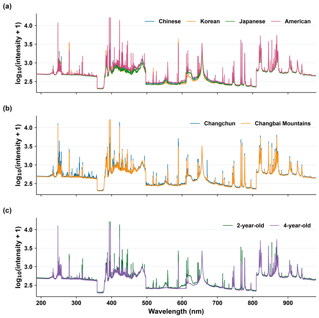
Figure 2.
Principal component analysis (PCA) score plots after standard normal variate preprocessing for (a) plant category, (b) geographical origin, and (c) growth year. Ellipses represent covariance dispersion at two standard deviations. Percentages indicate variance explained by the first two principal components.
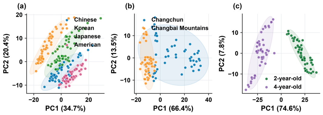
Figure 3.
Balanced accuracy of four classification pipelines for (a) plant category, (b) geographical origin, and (c) growth year. Symbols show means and error bars show standard deviations across 25 outer test folds from repeated nested cross-validation. PLS-DA, partial least-squares discriminant analysis; PCA, principal component analysis; RBF, radial basis function; SVM, support vector machine.
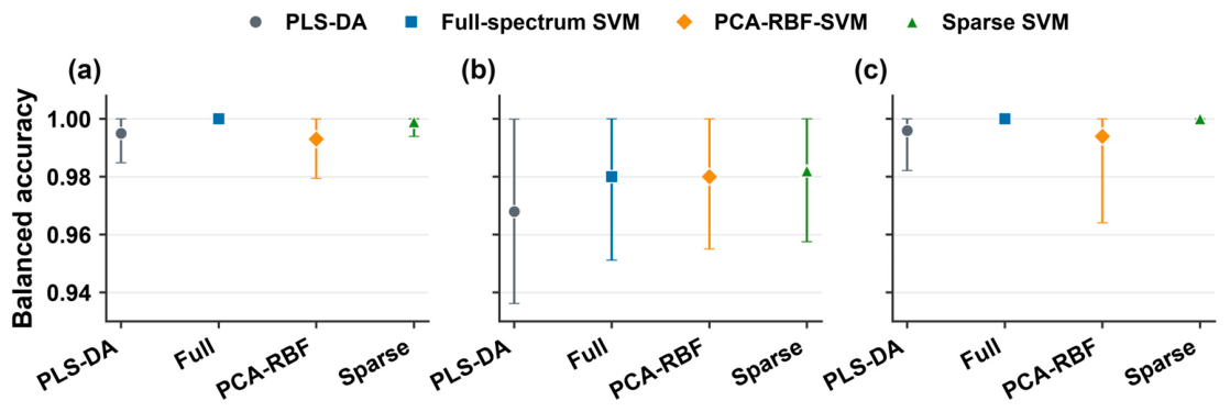
Figure 4.
Balanced accuracy after compression to 10–200 selected wavelengths. Points show means and error bars show standard deviations across 25 outer folds.
Figure 4.
Balanced accuracy after compression to 10–200 selected wavelengths. Points show means and error bars show standard deviations across 25 outer folds.
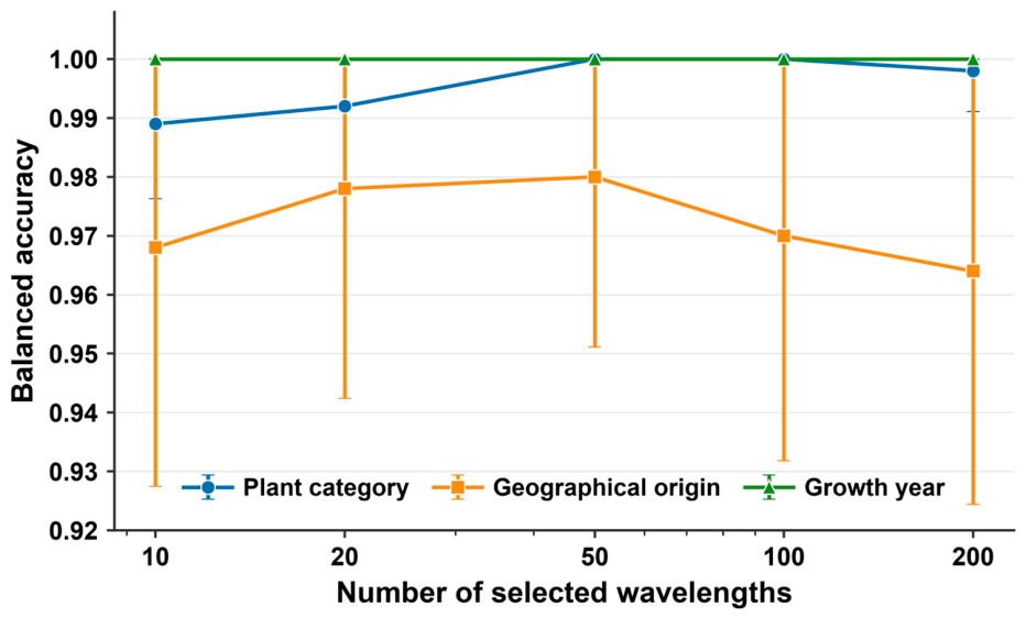
Figure 5.
Selection frequency of wavelength variables across 25 outer training folds for (a) plant category, (b) geographical origin, and (c) growth year. Gray lines mark selected detector channels, and colored points identify provisionally assigned candidate lines. Assignments are based on wavelength proximity and should not be interpreted as definitive elemental identification.
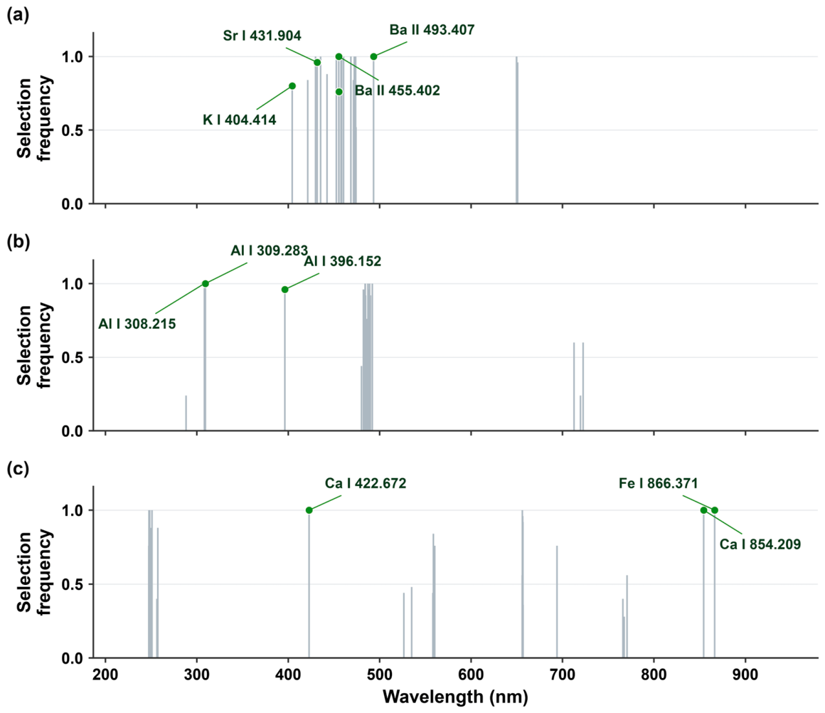
Figure 6.
Absolute balanced accuracy under computational perturbations applied only to held-out spectra. Columns show classification tasks, and rows show model–perturbation combinations. Shift values denote displacement by detector-channel indices; σ denotes Gaussian noise relative to signal variation. SNV, standard normal variate; SVM, support vector machine.
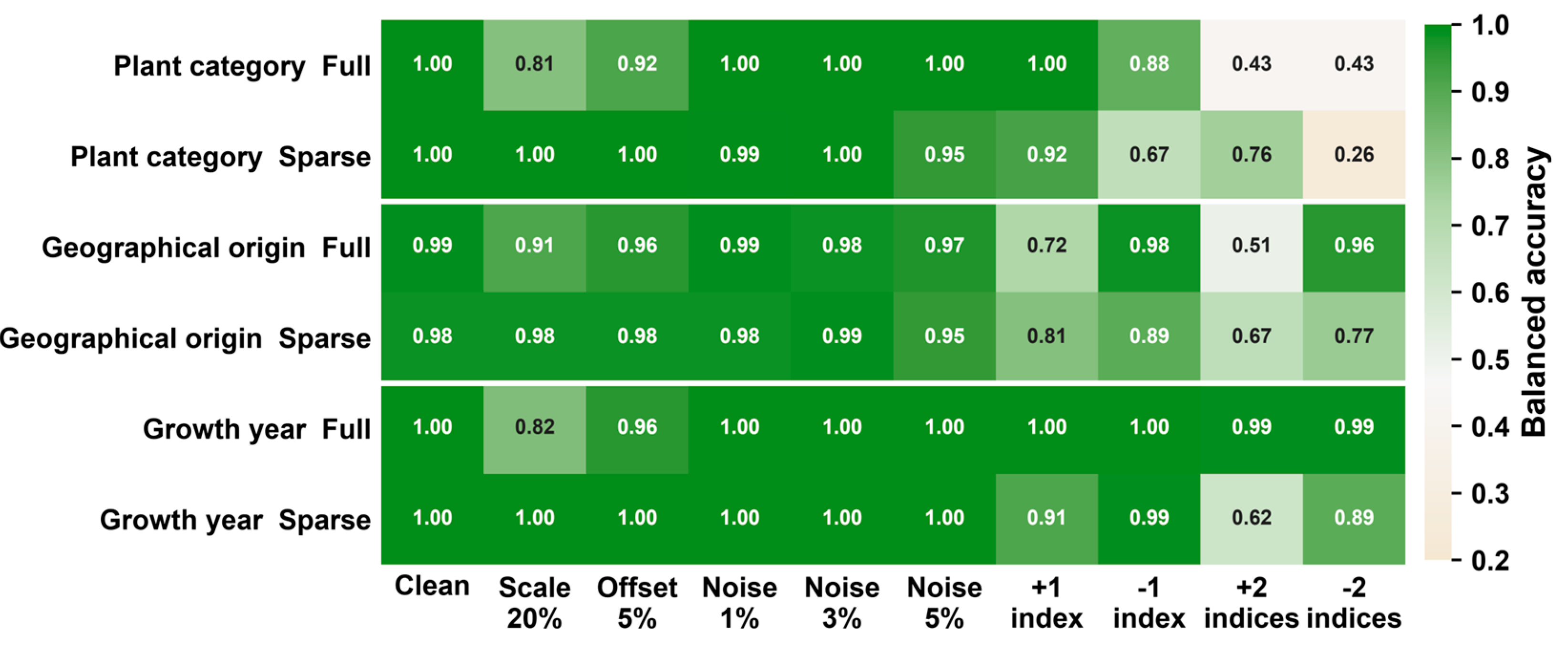
Table 1.
Repeated nested cross-validation performance (mean ± standard deviation across 25 outer folds).
Table 1.
Repeated nested cross-validation performance (mean ± standard deviation across 25 outer folds).
| Task | Model | Balanced accuracy | Macro-F1 | MCC |
|---|---|---|---|---|
| Plant category | Full-spectrum linear SVM | 1.000 ± 0.000 | 1.000 ± 0.000 | 1.000 ± 0.000 |
| PCA–RBF–SVM | 0.993 ± 0.014 | 0.993 ± 0.014 | 0.991 ± 0.017 | |
| PLS-DA | 0.995 ± 0.010 | 0.995 ± 0.010 | 0.993 ± 0.013 | |
| Sparse SVM | 0.999 ± 0.005 | 0.999 ± 0.005 | 0.999 ± 0.007 | |
| Geographical origin | Full-spectrum linear SVM | 0.980 ± 0.029 | 0.980 ± 0.029 | 0.962 ± 0.054 |
| PCA–RBF–SVM | 0.980 ± 0.025 | 0.980 ± 0.025 | 0.962 ± 0.048 | |
| PLS-DA | 0.968 ± 0.032 | 0.968 ± 0.032 | 0.939 ± 0.061 | |
| Sparse SVM | 0.982 ± 0.024 | 0.982 ± 0.025 | 0.966 ± 0.047 | |
| Growth year | Full-spectrum linear SVM | 1.000 ± 0.000 | 1.000 ± 0.000 | 1.000 ± 0.000 |
| PCA–RBF–SVM | 0.994 ± 0.030 | 0.994 ± 0.031 | 0.989 ± 0.053 | |
| PLS-DA | 0.996 ± 0.014 | 0.996 ± 0.014 | 0.992 ± 0.026 | |
| Sparse SVM | 1.000 ± 0.000 | 1.000 ± 0.000 | 1.000 ± 0.000 |
Table 2.
Balanced accuracy of sparse models as a function of the number of selected wavelengths.
| Task | 10 | 20 | 50 | 100 | 200 |
|---|---|---|---|---|---|
| Plant category | 0.989 | 0.992 | 1.000 | 1.000 | 0.998 |
| Geographical origin | 0.968 | 0.978 | 0.980 | 0.970 | 0.964 |
| Growth year | 1.000 | 1.000 | 1.000 | 1.000 | 1.000 |
Table 3.
Recurrently selected wavelengths and provisional candidate elemental assignments.
| Task | Selected (nm) | Frequency | Candidate line | Difference (nm) |
|---|---|---|---|---|
| Plant category | 493.282 | 1.00 | Ba II 493.407 | 0.125 |
| 455.256 | 1.00 | Ba II 455.402 | 0.146 | |
| 431.720 | 0.96 | Sr I 431.904 | 0.184 | |
| 404.314 | 0.80 | K I 404.414 | 0.100 | |
| Geographical origin | 309.314 | 1.00 | Al I 309.283 | 0.031 |
| 308.253 | 1.00 | Al I 308.215 | 0.038 | |
| 396.221 | 0.96 | Al I 396.152 | 0.069 | |
| Growth year | 422.711 | 1.00 | Ca I 422.672 | 0.039 |
| 854.379 | 1.00 | Ca I 854.209 | 0.170 | |
| 866.379 | 1.00 | Fe I 866.371 | 0.008 |
Disclaimer/Publisher’s Note: The statements, opinions and data contained in all publications are solely those of the individual author(s) and contributor(s) and not of MDPI and/or the editor(s). MDPI and/or the editor(s) disclaim responsibility for any injury to people or property resulting from any ideas, methods, instructions or products referred to in the content. |
© 2026 by the authors. Licensee MDPI, Basel, Switzerland. This article is an open access article distributed under the terms and conditions of the Creative Commons Attribution (CC BY) license.
Copyright: This open access article is published under a Creative Commons CC BY 4.0 license, which permit the free download, distribution, and reuse, provided that the author and preprint are cited in any reuse.