

Submitted:
01 October 2026
Posted:
05 October 2026
You are already at the latest version
Abstract
Continuous monitoring stations are the sensing layer of urban air-quality management, yet their records are often used to infer pollution “drivers” without controlling for weather. We ask what predicts fine particulate matter (PM2.5) in Navi Mumbai, a coastal Indian city, using screened daily data from five stations for 2021–2025, hourly data from two, and ERA5 reanalysis weather checked against Mumbai surface and radiosonde observations. Vector autoregressions with exogenous weather and calendar terms were estimated without imputation, together with hourly models, a stagnation index and out-of-sample forecasts. Lagged co-pollutants add little to daily prediction: equivalence tests bound six of seven effects within ±5% per standard deviation, while lagged ozone, an oxidant signal, raises PM2.5 by 4%. Omitting weather, or using PM10, manufactures co-pollutant “drivers”. Rainfall and boundary-layer height lower same-day PM2.5 by 10–24% per standard deviation, and date effects shared by all stations explain 78% of the variance, three-quarters of it weather. A stagnation index raises the frequency of days above the national standard two- to fourfold and, combined with persistence, warns as skillfully as an extreme gradient boosting (XGBoost) forecaster, which itself does not beat persistence. Monitoring data support citywide, meteorology-triggered warnings better than single-pollutant controls inferred from comovement.
Keywords:
PM2.5
; air-quality monitoring network
; early warning
; atmospheric stagnation
; boundary layer
; land–sea breeze
; Granger causality
; forecasting
; Navi Mumbai
1. Introduction
Fine particulate matter with an aerodynamic diameter of 2.5 µm or less (PM) is the air pollutant with the largest estimated health burden, acting through cardiovascular as well as respiratory pathways [1]. The World Health Organization guideline for the annual mean is 5 µg/m [2]; Indian cities routinely exceed the 24-hour National Ambient Air Quality Standard (NAAQS) of 60 µg/m [3]. For India, the Global Burden of Disease collaboration attributes about 1.67 million deaths in 2019 to air pollution, with output losses equal to 1.36% of GDP [4]. Satellite-based estimates put the national mean at 89 µg/m in 2015 and show that the ground monitoring network is too sparse and uneven to measure exposure in much of the country [5]. Pollution also lowers labor productivity [6], households spend on self-protection and state a willingness to pay for cleaner air [7,8], and Indian evidence on regulation shows that the design of air-quality policy matters for its effect [9]. Knowing which observable conditions precede high-PM days is therefore useful both for short-run warnings and for choosing where control effort goes.
Continuous Ambient Air Quality Monitoring Stations (CAAQMS) are the sensing infrastructure on which such decisions rest in Indian cities. Their hourly records feed public dashboards, city forecasts built on emission inventories and chemical transport models [10], and a growing number of statistical and machine-learning predictors, including for Navi Mumbai [11]. How much these records can support depends on their quality and on what can legitimately be inferred from them. A common empirical approach fits a vector autoregression (VAR) to daily concentrations of PM and co-pollutants, reads Granger causality tests, impulse responses and variance decompositions as evidence on sources, and adds a machine-learning forecaster. This approach has three weaknesses that are easy to overlook. The first is that pollutants co-move because they share weather: when the mixing layer is shallow and there is no rain, every locally emitted pollutant rises together. A VAR in which weather and season are either omitted or treated as endogenous will attribute this common movement to the pollutants themselves. The second is definitional overlap. PM includes PM, and NO is approximately the sum of NO and NO, so including these series side by side produces mechanical predictive relations and unstable coefficients; the two particle fractions are so closely related that PM is routinely estimated from PM where it is not measured [12]. The third concerns data. Continuous monitors stall, drift and go offline; filling gaps by carrying values forward or backward inflates measured persistence and, for forecasting, lets future information leak into the inputs. Imputation before modeling is nonetheless common in air-quality forecasting [13,14].
The Granger test [15], usually applied within a VAR [16], asks whether the past of one series improves the prediction of another given the past of the others. It measures incremental predictive content, not physical causation, and its outcome depends on what else is in the information set. That dependence matters because causal language is now common in studies of PM [17], and because the information usually omitted is weather, which drives both dispersion and chemical formation [18]. Closest to our approach, Aganović and Kadrić [19] screen predictors with Granger tests inside autoregressive models with exogenous meteorology for Sarajevo and find wind speed and temperature to be the strongest short-run drivers. The weather signal is large. Temperature, wind, humidity, precipitation and mixing height each move PM in chemical transport simulations [20]; long-run weather changes alone have raised or lowered pollutant levels [21,22]; the representation of boundary-layer mixing largely decides whether winter particulate peaks are reproduced [23]; and meteorology affects the coarse and fine fractions differently [24]. Meteorological normalization removes this signal before analyzing trends or interventions [25,26,27]. In coastal cities the land–sea breeze adds a diurnal circulation that can carry pollutants offshore at night and back onshore by day [28,29], and it interacts with urban areas in ways that reanalyses resolve poorly [30]. On India’s west coast the sea breeze is a regular dry-season feature [31]. For Mumbai and Navi Mumbai, source-apportionment studies identify industrial, vehicular, road-dust and combustion sources in fine and coarse particles [32,33,34]. Elsewhere in India, wet scavenging lowers particle levels in the monsoon, while stagnation, local activity and biomass burning raise them afterwards [35,36]. Machine-learning forecasts of PM report high accuracy for many cities [37,38,39,40,41,42], including Hyderabad and Kolkata [43,44], but accuracy is not always measured out of sample with time-ordered splits, or against persistence, which is a demanding benchmark for a strongly autocorrelated series; tests of equal predictive accuracy [45,46] allow formal comparison. Finally, monitoring data quality is itself an economic question, since manipulated or faulty records can bias policy evaluation [47].
This paper revisits the question for Navi Mumbai, a planned city in the Mumbai Metropolitan Region with a large chemical and engineering industrial belt along the Thane–Belapur road, with a design that addresses each of these problems. We use daily data for 2021–2025 from five stations of the Central Pollution Control Board (CPCB) network, and hourly data from two of them. Mahape lies in the industrial belt; Nerul, Sector-19A Nerul, Kopripada-Vashi and Sanpada lie in mixed residential and commercial areas. Pollutant records are screened for stalled analyzers, non-positive values and physically inconsistent days, and missing days are left missing. Weather comes from the fifth-generation atmospheric reanalysis of the European Centre for Medium-Range Weather Forecasts (ERA5) [48], which provides rainfall and boundary-layer height (BLH) that the monitoring stations do not measure reliably, and which we check against surface observations at Santacruz and the Mumbai radiosonde. The coarse fraction PM replaces PM, NO represents nitrogen oxides, and wind enters as vector components rather than degrees. The econometric model is a VAR with exogenous variables (VARX) in which pollutants are endogenous and weather, season, day of week, year, the 2021 lockdown and Diwali are exogenous. Granger tests use heteroskedasticity-robust Wald statistics with Holm’s adjustment for multiple testing [49], and dynamics are summarized with order-invariant generalized impulse responses and variance decompositions [50,51]. Forecasts from extreme gradient boosting (XGBoost) [52] are compared out of sample with persistence, climatology, a linear model with the same inputs and the VARX itself, using Diebold and Mariano [45] (DM) tests, and a simple stagnation index is evaluated as a warning trigger.
The results change the picture that the uncontrolled approach produces. At Mahape, lagged PM and weather account for nearly all of the explained daily variation. The seven lagged co-pollutants are jointly significant but add only 2% to the explained variance, and for six of them equivalence tests bound the effect of a one-standard-deviation (SD) increase on next-day PM within ±5%; lagged ozone is the exception. Without the weather and calendar controls, NO and SO become significant predictors, and with PM instead of the coarse fraction the share of PM forecast-error variance attributed to other variables rises by about 15 percentage points. Hourly data qualify the picture: coarse particles and CO lead PM within the day, but their effects cancel over 24 hours. Across the five stations, rainfall and boundary-layer height lower same-day PM by 10–24% per standard deviation, date effects common to all stations explain 78% of the variance, and weather explains about three-quarters of these date effects. Days with a regional land–sea breeze raise daily PM at Nerul by 9%. A simple stagnation index raises the frequency of exceedance days two- to four-fold and, combined with persistence, warns as skillfully as XGBoost, whose accuracy is statistically indistinguishable from that of persistence at every station.
The paper contributes in three ways. It shows, with a direct comparison of specifications, how much of the co-pollutant “driver” evidence in VAR studies of urban air quality can be produced by omitted weather and by overlapping measures. It documents data-quality problems in CAAQMS records that matter for any use of these data, including a benzene analyzer at Mahape that reported the same value for most of 2025. And it evaluates machine-learning forecasts and a meteorological stagnation index against the benchmarks that matter for operational warnings in a city, rather than reporting in-sample fit. Section 2 describes the data and methods, Section 3 reports the results, Section 4 discusses their interpretation, limits and use in city air-quality management, and Section 5 concludes. Tables and figures numbered with the prefix S are in the Supplementary Materials.
2. Materials and Methods
2.1. Study Area and Monitoring Network
Daily (24-hour) averages for 1 January 2021 to 31 December 2025 were downloaded from the CPCB Central Control Room data repository for every CAAQMS in Navi Mumbai except Sector-2E Kalamboli and Taloja, which lie in the Panvel area outside the Navi Mumbai Municipal Corporation (NMMC) and are excluded by design. Of the six remaining stations, Airoli is excluded. The repository lists hourly as well as daily files for Airoli for 2021–2025, but both contain no pollutant or meteorological measurements for the study period; the last valid readings date from 9 April 2020. With no daily series available, the station cannot enter the analysis. Mahape and Nerul report over the whole period; Sector-19A Nerul, operated by the Indian Institute of Tropical Meteorology (IITM), reports until November 2024; Kopripada-Vashi and Sanpada start in June 2023. The other stations are operated by the Maharashtra Pollution Control Board (MPCB). Table 1 gives, for each station, the length and coverage of the PM record, its mean, median and 90th percentile (P90), and the share of days above the NAAQS. Mahape is the main station for the detailed analysis because it has the longest and most complete record and the only usable benzene series. For Mahape and Nerul we also downloaded hourly averages; after screening, PM is available for 36,262 and 36,176 hours, 83% of all hours. Ozone at Nerul is missing for most of 2021, 2023 and 2025 and is not used there. The CPCB repository does not publish the make or measurement principle of the particulate monitors (Table 2), so we cannot correct for humidity-dependent measurement error.
Figure 1 maps the stations within the NMMC boundary from OpenStreetMap, together with the Thane–Belapur (TTC) industrial belt of the Maharashtra Industrial Development Corporation (MIDC), the mangrove fringe of Thane Creek, the main transport corridors and the ERA5 grid cell used for meteorology; Table 2 gives coordinates and distances to the creek shoreline, industrial land and major roads. Mahape lies in the north, next to the industrial belt; Kopripada-Vashi, Sanpada and the two Nerul stations lie in the residential and commercial nodes further south.
All stations share the same seasonal cycle, with winter means of 60–110 µg/m and monsoon means of 15–24 µg/m (Figure 2).
2.2. Data Screening
Daily means of zero or below are set to missing; a run of identical daily means on three or more consecutive days is treated as a stalled analyzer and set to missing; and days on which PM exceeds PM are set to missing for both fractions (Table S1). The rules remove few values for most pollutants but 393 of 1,769 benzene values at Mahape, where the analyzer reported exactly 2.37 µg/m from March to December 2025 and for long stretches in 2023 (Figure 3); benzene is therefore used only until February 2025, and a variant without it is reported. Missing values are never imputed. Hourly records are screened in the same way, with a stalled analyzer defined as six or more identical hours.
2.3. Meteorology and Calendar
The station weather sensors are incomplete and in places implausible (at Mahape, wind speed reaches 49.9 m/s and rainfall is zero on every day). We therefore use hourly ERA5 reanalysis [48] from the Open-Meteo archive for the grid point at 19.00N, 73.00E, aggregated to daily rainfall and mean boundary-layer height, temperature, relative humidity and zonal (u) and meridional (v) wind, with and for speed W and direction , so that positive u is a westerly (onshore) wind. All analyzed stations lie inside the grid cell (Figure 1). The archive lacks boundary-layer height from January to June 2024; we fill it from a regression on the other ERA5 variables (out-of-sample ) and show that excluding the period changes nothing (Table S14).
We check ERA5 against hourly synoptic reports from the India Meteorological Department station at Santacruz, World Meteorological Organization (WMO) station 43003, distributed by Meteostat, and against the afternoon mixed-layer height of the Mumbai radiosonde [53], launched at 12:00 Coordinated Universal Time (UTC), which is 17:30 Indian Standard Time (IST), (Table S17, Figure S5). ERA5 reproduces daily temperature (, 1.1C too cool), humidity (), wind speed () and monthly rainfall (, about 30% too low). Its boundary-layer height agrees poorly with the radiosonde (, 340 m lower), in line with evaluations over the Indian monsoon region [54]; the 17:30 sounding also samples a boundary layer that is already collapsing, and radiosonde-derived heights depend on the retrieval method [55]. We therefore repeat the boundary-layer analyses with the radiosonde mixing height (Section 3.3).
The calendar terms are month, day-of-week and year effects, a dummy for the Maharashtra COVID-19 restrictions of 14 April to 14 June 2021, and a dummy for the five days centered on Diwali. Summary statistics are in Table S2.
2.4. The VARX Model
Throughout, bold symbols denote vectors and matrices and italic symbols denote scalars. Let be the k-vector of log pollutant concentrations on day t; at Mahape it contains PM, the coarse fraction PM, NO, CO, SO, O, NH and benzene (). The model is
where p is the lag order, a vector of intercepts, the coefficient matrices of the lagged pollutants, and the coefficient matrices of current and lagged weather, the coefficient matrix of the calendar terms and the error vector with covariance matrix ; holds the six weather variables (rainfall as , log boundary-layer height, temperature, humidity, u, v), the calendar terms, and the information set of lagged pollutants with current and lagged weather and calendar terms. Weather is exogenous because daily pollution does not affect the next day’s weather at this scale. The coarse fraction replaces PM, which contains PM by definition, and has sources of its own such as resuspension [56]; only NO represents the nitrogen oxides, since NO is approximately NO plus NO; and benzene represents the aromatic compounds.
The system is estimated equation by equation by ordinary least squares. A day enters only if all elements of and of , are observed, which keeps every lag at its true calendar distance and uses no imputed or future values. The lag order is chosen by the Bayesian information criterion (BIC) over ; residual autocorrelation is checked with Breusch–Godfrey-type tests at lags 1 and 7 and Ljung–Box statistics. Augmented Dickey–Fuller (ADF) [57] and Kwiatkowski–Phillips–Schmidt–Shin (KPSS) [58] tests reject a unit root for every series (Table S8); because unit-root inference is fragile we also report Toda and Yamamoto [59] Granger tests.
2.5. Granger Tests, Effect Bounds and Dynamics
Variable j does not Granger-cause PM if
where is element of . We use heteroskedasticity-robust (HC1) standard errors (SE) and Wald tests, since PM shows volatility clustering [60], and adjust for testing seven co-pollutants with the methods of Holm [49] and Benjamini and Hochberg [61] (BH). A failure to reject is not evidence of no effect, so we express each summed lag coefficient as the percentage change in next-day PM after a one-standard-deviation increase in the log pollutant, , where is the standard deviation of the log pollutant, and test equivalence with the two one-sided tests (TOST) procedure [62]: rejecting the null that the effect lies outside ±5% per standard deviation establishes that it is small.
Dynamics are summarized with generalized impulse response functions (GIRF) and forecast-error variance decompositions (GFEVD), which do not depend on the order of the variables [50,51,63]. With and , the response to a one-standard-deviation shock in variable j is
where is the jth diagonal element of and the jth column of the identity matrix, and the share of the H-step forecast-error variance of variable i due to shocks in j is
normalized to sum to one. Weather effects are summarized by dynamic multipliers,
where and are the k-th columns of and and . To separate an oxidant signal from ozone titration by fresh NO emissions, the ozone results are repeated with odd oxygen, O = O + NO (in ppb), which is conserved under titration.
2.6. Other Stations, City-Wide Effects and Hourly Data
For the station comparison we use six pollutants (PM, PM, NO, CO, SO, O) available at all stations. A pooled equation with station and date fixed effects identifies co-pollutant effects only from differences between stations on the same day; the estimated date effects, which capture everything the stations share, are then regressed on ERA5 weather and calendar terms, weighted by the number of stations reporting.
For Mahape and Nerul the VARX is also estimated on hourly data, with hourly ERA5 variables and hour-of-day, day-of-week, month, year and event terms. The lag order is chosen by BIC over 1 to 48 hours, and if the residuals of the PM equation remain autocorrelated at the daily cycle (Ljung–Box ) we use the smallest order that removes it. Hourly Granger tests ask whether a co-pollutant leads PM within the day; the sum of the lag coefficients measures whether that lead changes the daily level.
A day is classified as a land–sea (creek) breeze day when it is dry (ERA5 rainfall below 1 mm), the mean ERA5 zonal wind is offshore () between 00:00 and 07:00 IST and onshore () between 12:00 and 17:00 IST, and u rises by at least 1 m/s between the two periods. West of the stations lie Thane Creek and Mumbai harbour rather than open sea, and the 0.25 reanalysis resolves only the regional circulation, so the rule identifies days with a regional land–sea breeze regime. We compare it with the same rule applied to Santacruz and to station winds, and estimate its effect with a dummy in a daily regression of log PM on its lag, weather and calendar terms (Newey–West standard errors).
2.7. Stagnation Index and Forecasts
A day is stagnant when ERA5 boundary-layer height and wind speed are both below their 2021–2024 33rd percentiles and rainfall is below 1 mm; the ventilation coefficient (daily mean of boundary-layer height times wind speed) is its continuous counterpart. For next-day PM we compare XGBoost [52], which minimizes
over regression trees with leaves and weights ; is PM on day t in µg/m, its forecast, the complexity penalty of a tree, and and regularization parameters. XGBoost is compared with persistence (), monthly climatology, a linear autoregression with exogenous variables (ARX) on the same inputs and the VARX(1) PM equation. Inputs are lags 1, 2, 3 and 7 of the six pollutants, ERA5 weather on day and, in the main setting, on day t (a perfect weather forecast), and calendar terms; no same-day pollutant enters and missing inputs are not imputed. Hyperparameters are tuned by time-ordered cross-validation (CV) on the training data. The test year is 2025 (2024 for Sector-19A Nerul), with all models re-estimated each month on all earlier data. We report the root mean squared error (RMSE) and mean absolute error (MAE) [64], Diebold and Mariano [45] tests with the Harvey et al. [46] correction and a Newey–West variance [65], and SHapley Additive exPlanations (SHAP) importance [66]. Warnings for days above 60 µg/m are scored by the probability of detection (POD), the false-alarm ratio (FAR) and the Peirce skill score (PSS), with 90% intervals from a moving-block bootstrap (7-day blocks), and the ventilation coefficient by the area under the receiver operating characteristic (ROC) curve (AUC).
2.8. Software
All computations were carried out in Python 3.14.7 with pandas 3.0.5, NumPy 2.5.2, SciPy 1.18.0, statsmodels 0.14.6, scikit-learn 1.9.0, XGBoost 3.4.1, SHAP 0.52.0 and Matplotlib 3.11.1. The VARX estimator, the Granger and equivalence tests, the generalized impulse responses and variance decompositions, and the bootstrap were written by the authors; maps were drawn from OpenStreetMap layers retrieved through the Overpass application programming interface. The code is available as described in the Data Availability Statement.
3. Results
3.1. Daily Co-Pollutant Effects at Mahape
BIC selects one lag. The PM equation then has serially uncorrelated residuals (Ljung–Box ) and the system is stable (largest companion eigenvalue 0.945; Tables S4 and S5). The sample has 1,092 days from January 2021 to February 2025. PM is persistent (own-lag coefficient 0.68) and the equation explains 86% of the daily variation in log PM (Table S6).
Table 3 reports the co-pollutant tests (the Wald statistics and Toda–Yamamoto versions are in Table S3). For six of the seven co-pollutants (coarse particles, NO, CO, SO, NH and benzene) the equivalence tests establish that a one-standard-deviation increase changes next-day PM by less than 5% (), with point estimates between % and %. Ozone is the exception: % per standard deviation (95% confidence interval (CI) to %), significant after the Holm adjustment () and in the Toda–Yamamoto test (). The seven co-pollutants are jointly significant (, ) but add only 2.1% to the explained share of the remaining variance. At the other stations NO is bounded within ±5% everywhere and the joint block is significant only at Mahape.
Lagged ozone could predict PM because it marks oxidant and photochemical activity, or because fresh NO emissions titrate ozone, so that low ozone signals high local emissions. Odd oxygen separates the two (Table S10). At Mahape the effect survives, and grows, when O replaces O (% per standard deviation, 95% interval to %) or replaces both O and NO (%). It is concentrated in the dry season (%, against % and insignificant in the monsoon; test of equality ). At Kopripada-Vashi lagged O is marginal (%, ) but O is clearly positive (%); at Sanpada and Sector-19A Nerul neither is significant. The ozone result is therefore consistent with oxidant-driven secondary aerosol formation rather than with titration, though it cannot exclude synoptic conditions that raise both.
3.2. What the Controls and the Coarse Fraction Change
Table 4 estimates four specifications on the same 1,092 days. With PM and no exogenous terms (column A), lagged NO (), SO () and O () all predict PM. Replacing PM by the coarse fraction (B) leaves these tests nearly unchanged but raises the own share of PM in its 10-day forecast-error variance from 51% to 66%: fifteen percentage points that (A) credits to PM belong to the PM inside it. Calendar terms (C) remove the significance of NO and SO, which follow the weekly and seasonal cycles, and weather (D) raises the own share to 75%. With five lags the own share rises in the same way (51%, 66%, 68% and 73%). Much of the co-pollutant evidence in an uncontrolled VAR therefore reflects shared seasonal and weather variation and definitional overlap.
3.3. Weather
Weather is strongly significant as a block (, ; Table 5). A one-standard-deviation increase in rainfall lowers same-day PM by 14%, consistent with wet removal [36], and a one-standard-deviation deeper ERA5 boundary layer lowers it by 16%, with a partial rebound the next day. On the 457 days with a radiosonde sounding, the radiosonde mixing height also lowers PM significantly, by 6% per standard deviation, against 16% for ERA5 on the same days (Table S18); the direction is robust, the magnitude depends on the boundary-layer data, and the co-pollutant results are unchanged. Temperature has offsetting same-day and lagged coefficients, as in other cities where its sign varies by season [67]; humidity is insignificant. A westerly ERA5 wind component is associated with 7% higher PM at Mahape per standard deviation. We do not interpret its source: the Mahape anemometer, whose record is unreliable, shows a weak easterly mean afternoon wind ( m/s), so the regional westerly need not be the flow at the station. The 2021 restrictions lowered PM by about 13% and the Diwali window raised it by about 14%. These are associations conditional on the model, which cannot separate dispersion from secondary formation [18].
Generalized impulse responses and variance decompositions (Figures S1 and S2, Table S9) tell the same story. PM’s own innovations account for 75–77% of its forecast-error variance at horizons of 1 to 20 days, coarse particles for about 7% and ozone for 6% at 10 days; with PM ordered first its own share is 94%, so most of the other shares reflect contemporaneous co-movement. Only the ozone response builds up after impact, peaking at about 3.4% after one to three days.
3.4. Hourly Dynamics and the Land–Sea Breeze
In winter, PM falls to 0.71 of its daily mean at Mahape at 14:00 and to 0.65 at Nerul at 17:00, when the boundary layer is deepest (Figure 4). At Mahape, beside the industrial belt, PM peaks at 22:00 (1.30 times the daily mean), together with CO (21:00) and NO (19:00), as the evening boundary layer collapses over evening emissions; at Nerul the peak is at 09:00 (1.42), with CO and NO in the morning traffic period. Ozone at Mahape peaks in the late afternoon, out of phase with PM. In the monsoon all profiles flatten.
Table 6 reports the hourly VARX. At Nerul BIC selects 30 hourly lags and the residuals are white (). At Mahape BIC selects 6 lags, but the residuals then remain autocorrelated at the daily cycle (), so we use 24 lags (); with 6 lags the co-pollutants are also jointly significant (, ). At this resolution every co-pollutant leads PM (joint at Mahape and at Nerul, each pollutant significant after adjustment). With 13,000–16,000 hours significance is easy to reach, so the effect sizes matter more. Coarse particles and CO carry most of the information, accounting for 15% and 7% of the 24-hour-ahead forecast-error variance of PM at Mahape and 6% and 14% at Nerul. Their summed effects are small and mostly negative ( for coarse particles at Mahape, for CO at Nerul). Figure S4 shows why: the first-hour coefficient is positive and large (0.15 for coarse particles and 0.18 for CO at Mahape), most of it is reversed in the second hour, and the cumulative effect drifts to about zero by 24 hours. At Nerul the CO lag coefficients alternate in sign from hour to hour, so individual CO lags are poorly determined there even though their sum is not. Co-pollutants therefore shape the timing of PM within the day, largely through the shared diurnal cycle of emissions and mixing, but not its daily level.
By the ERA5 rule, land–sea breeze days make up 55% of October–May days (81% in December) and almost none from June to September (Figure 5). Conditional on the lag of PM, weather and calendar, they raise daily PM by 9.0% at Nerul () and by 2.6% at Mahape (; Table S11). The classification agrees with the same rule applied to Santacruz winds on 71% of days (Cohen’s ), but hardly at all with the station anemometers (–). At Nerul, 0.8 km from the creek shoreline, the station wind is westerly both at night (1.1 m/s on average) and in the afternoon (2.5 m/s), so locally the regime appears as an afternoon strengthening of creek-side westerlies rather than a full reversal. The result therefore concerns days with a regional land–sea breeze. The larger effect at Nerul may reflect recirculation of pollution by the onshore flow, but the data cannot test that mechanism.
3.5. All Stations
Station-by-station VARX models (Table S12) confirm the Mahape picture: BIC selects one lag everywhere, own persistence is high (sum of own lags 0.55–0.83), PM’s own share of its 10-day forecast-error variance ranges from 69% to 88%, rainfall and boundary-layer height lower same-day PM by 10–24% per standard deviation at every station, and after adjustment the only co-pollutant with predictive content is the coarse fraction at Mahape, with a negative coefficient. Figure 6 maps these estimates. Levels and exceedances are highest at Sector-19A Nerul and Nerul and lowest at Mahape, while persistence, the weather effects and the forecasting gain vary without a clear spatial pattern. Correlation of daily PM between stations does not decline with distance (Figure 7): Mahape and Nerul, 11.6 km apart, correlate more closely (0.73) than Mahape and Kopripada-Vashi at 2.6 km (0.69). The three central and southern MPCB stations move most closely together (0.82–0.85), whereas every pair involving Mahape or the IITM station correlates at 0.53–0.73, pointing to local sources at Mahape or differences in instruments rather than distance.
In a pooled equation with station and date fixed effects no co-pollutant remains significant after adjustment (Table S13). Date effects common to all stations account for 78% of the variance of daily log PM, station effects for 1%. Table 7 splits the date effects. ERA5 weather on the day and the day before explains 73% of their variance and weather plus calendar 79%; nonlinear terms add little, and an out-of-sample gradient-boosting model reaches 66%. About one-fifth of the common daily variation, some 16% of the total variance, is common to the city but not explained by weather or calendar; it combines city-wide emission shocks, regional transport and reanalysis error, which the data cannot separate.
The Mahape results are robust to two, three or eight lags, NO instead of NO, an aromatic index instead of benzene, dropping benzene to extend the sample, interpolating short gaps and excluding the gap-filled boundary-layer period (Table S14): no co-pollutant other than ozone and, in two variants, the coarse fraction and CO is significant after adjustment.
3.6. Forecasts
On the 346 test days at Mahape on which XGBoost and persistence can both be evaluated, XGBoost with same-day weather has an RMSE of 6.84 µg/m against 7.07 for persistence and 21.9 for climatology (Table 8). The difference from persistence is not significant (); with lagged weather only XGBoost is marginally worse than persistence (). On the 176 days with complete inputs, persistence has the lowest RMSE (4.82), followed by the VARX equation (5.01), XGBoost (5.76) and the linear model (6.37). XGBoost over-predicts in the cleaner months by 3–5 µg/m (Table S16, Figure 8), because mean PM at Mahape fell from 58 µg/m in 2021 to 27 in 2025 and the series became much smoother; we cannot tell whether that reflects cleaner air or a change in the instrument. At the other stations XGBoost is within 1.8 µg/m of persistence and never significantly better at 5% (Table S15). Lagged PM, same-day rainfall and boundary-layer height dominate its inputs (Figure S3).
3.7. A Stagnation Index as a Warning Trigger
Stagnant days (boundary-layer height below 331 m, wind speed below 2.4 m/s, no rain) make up 15% of all days and 29% of November–February days. On them PM exceeds 60 µg/m on 48–72% of days, against 13–30% otherwise, a two- to four-fold increase at every station (Figure 9), and the ventilation coefficient discriminates exceedance days with an AUC of 0.75–0.88 (Table 9). On its own, the binary index detects 37% of exceedance days across the stations (PSS 0.28, 90% interval 0.23–0.34) and is weaker than persistence (0.62, 0.55–0.68). Combined with persistence, issuing a warning when the day is forecast to be stagnant or yesterday exceeded the standard, it detects 81% of exceedance days with a PSS of 0.66 (0.60–0.71), practically the same as XGBoost (0.65, 0.59–0.72) but with more false alarms (FAR 0.42 against 0.28). Using yesterday’s weather lowers the skill of the stand-alone index by up to 0.11. Built from the radiosonde mixing height instead of ERA5, the index still raises exceedance frequency but discriminates less well (AUC 0.53–0.69 against 0.73–0.76 on the same days; Table S18).
4. Discussion
The main daily finding is negative in a useful sense. Once weather and calendar structure are held constant, the previous day’s concentrations of other pollutants add little to the prediction of daily PM in Navi Mumbai, and for most of them the data bound the effect within a few percent. The strong co-pollutant effects of an uncontrolled VAR reflect shared weather and seasons, the PM contained in PM and, at Mahape, a stalled benzene analyzer. Within the day, coarse particles and CO do lead PM, but these leads cancel over 24 hours. City-wide daily effects dominate, and weather explains about three-quarters of them.
This does not mean that local emissions are unimportant. Daily Granger tests at a monitor cannot detect sources whose emissions change slowly: a steady industrial or traffic source raises the level of PM, which station and year effects absorb, without creating day-to-day predictive content. Such level differences are what cross-city studies of socioeconomic and industrial drivers explain [68,69]. The lagged-ozone result is more informative: ozone marks photochemical activity, and a rise preceding higher PM is consistent with secondary aerosol formation from industrial and traffic precursors, but ozone may also signal synoptic conditions the reanalysis misses, so it is a leading indicator rather than a source.
For the management of city air quality, the results argue against single-pollutant targets chosen from co-movement statistics. Controls on road dust, traffic and industrial volatile organic compounds are supported by source-apportionment evidence [33,34], not by the Granger tests reported here. What the monitoring data do support is operational. Because rainfall, boundary-layer height and persistence account for most of the predictable variation, short-run warnings and temporary restrictions should be triggered by forecasts of stagnant, dry conditions and applied city-wide. A rule as simple as “stagnant tomorrow or above the standard today” is as skillful as a tuned machine-learning forecaster, at the cost of more false alarms, and it can be computed from a weather forecast and the previous day’s network data without a trained model. Forecast-triggered schemes work only if their rules are applied consistently [70]. The thresholds here are defined on ERA5 boundary-layer height, whose estimated effect is about 2.5 times the radiosonde-based estimate; an operational index would have to be recalibrated on the boundary-layer height of the forecast model that issues the warning. The evening peak at Mahape and the morning peak at Nerul indicate when within the day such measures would matter most, and any statistical forecaster should be re-trained often, since one trained on earlier years over-predicted when concentrations fell in 2025. For the monitoring network itself, the screening results argue for automated checks on stalled analyzers and physically inconsistent values before data are published or used in warnings, and for publishing instrument metadata with the data.
Several limitations remain. Granger causality is predictive, not causal. A single reanalysis cell cannot represent street-level ventilation or the local creek breeze, and although ERA5 surface weather agrees well with observations, its boundary-layer height agrees poorly with the radiosonde; the boundary-layer effect is robust in sign but not in size. The breeze classification is regional and is not confirmed by the station anemometers, whose siting and quality are unknown. The hourly analysis covers two stations, the forecasts and warnings are evaluated on one test year, and the screening rules cannot detect drift or calibration errors. Because the monitor types are not published, humidity artifacts in the particle measurements cannot be ruled out; relative humidity enters every model, but that controls for its atmospheric effect, not for a measurement bias. Speciated PM, emission inventories or chemical transport modeling would be needed to attribute concentrations to sources.
5. Conclusions
Using screened daily data from five monitoring stations in Navi Mumbai for 2021–2025, hourly data from two of them and ERA5 weather checked against Mumbai observations, we estimated VARX models that treat weather and calendar effects as exogenous, use the coarse fraction instead of PM, avoid overlapping nitrogen-oxide measures and impute no missing values. PM is persistent and strongly shaped by rainfall and the boundary layer. At the daily scale, lagged co-pollutants add little: their effects are bounded within ±5% per standard deviation for most pollutants, although the group is jointly significant and ozone at Mahape remains a leading indicator of oxidant conditions. At the hourly scale co-pollutants lead PM within the day without changing its daily level. Uncontrolled specifications, or specifications with PM, produce much stronger co-pollutant evidence, which should not be read as source attribution. City-wide daily effects dominate and weather explains most of them; days with a regional land–sea breeze raise PM at Nerul; and a stagnation index combined with persistence is as skillful a warning rule as XGBoost, which itself beats climatology but not persistence. Better attribution will require speciated measurements and emission data; better short-run management can already use the weather.
Supplementary Materials
The following supporting information can be downloaded at the website of this paper posted on Preprints.org, Figure S1: Generalized impulse responses of PM to one-standard-deviation shocks, Mahape VARX(1); Figure S2: Generalized forecast-error variance decomposition of PM by horizon, Mahape VARX(1); Figure S3: Mean absolute SHAP values of the 15 most important XGBoost inputs, Mahape, 2025 test year; Figure S4: Cumulative lag coefficients of co-pollutants in the hourly PM equation (sum of the coefficients on lags 1 to k), Mahape (24 lags) and Nerul (30 lags); Figure S5: ERA5 against Mumbai observations, 2021–2025: daily mean temperature and monthly rainfall at Santacruz (IMD 43003), and the 17:30 IST mixed-layer height of the Mumbai radiosonde (excluding January–June 2024); Table S1: Data screening at Mahape, 2021–2025 (1,826 days); Table S2: Summary statistics, Mahape station and ERA5 meteorology; Table S3: Granger tests in the PM equation, Mahape VARX(1); Table S4: Lag-order selection, Mahape VARX; Table S5: Residual diagnostics of the Mahape VARX; Table S6: Full PM equation of the Mahape VARX(1); Table S7: Granger p-values for all equations of the Mahape VARX(1); Table S8: Unit-root and stationarity tests, Mahape; Table S9: Forecast-error variance decomposition of PM and cumulative responses, Mahape; Table S10: Lagged ozone and odd oxygen (O) in the PM equation; Table S11: Land–sea breeze days and daily PM; Table S12: Station-by-station VARX with a common variable set; Table S13: Pooled PM equation across the five stations; Table S14: Robustness of the Mahape results; Table S15: One-day-ahead forecast RMSE by station (µg/m); Table S16: Forecast RMSE (bias) by season, Mahape, 2025; Table S17: ERA5 against Mumbai observations, 2021–2025; Table S18: Robustness to the boundary-layer data: ERA5 against the Mumbai radiosonde.
Author Contributions
Conceptualization, S.R.D. and S.K.K.; methodology, S.R.D.; software, S.R.D.; validation, S.K.K.; formal analysis, S.R.D.; investigation, S.R.D. and S.K.K.; data curation, S.R.D.; writing—original draft preparation, S.R.D.; writing—review and editing, S.K.K.; visualization, S.R.D.; supervision, S.K.K.; project administration, S.K.K. All authors have read and agreed to this version of the manuscript.
Funding
This research received no external funding.
Institutional Review Board Statement
Not applicable.
Informed Consent Statement
Not applicable.
Data Availability Statement
The data analyzed in this study were derived from the following resources available in the public domain: daily and hourly CAAQMS data from the Central Pollution Control Board Central Control Room repository (https://airquality.cpcb.gov.in/ccr/); ERA5 reanalysis from the Open-Meteo historical weather archive (https://open-meteo.com/); Santacruz (WMO 43003) surface observations from the Meteostat bulk archive (https://meteostat.net/); radiosonde-derived mixing heights from the NOAA Integrated Global Radiosonde Archive, station INM00043003 (https://www.ncei.noaa.gov/products/weather-balloon/integrated-global-radiosonde-archive); and map layers from OpenStreetMap (https://www.openstreetmap.org/). The screened daily and hourly panels and the Python code that produces every table and figure are available from the corresponding author on request and will be deposited in a public repository with a persistent identifier upon publication.
Conflicts of Interest
The authors declare no conflicts of interest.
References
- Krittanawong, C.; Qadeer, Y.K.; Hayes, R.B.; Wang, Z.; Thurston, G.D.; Virani, S.; Lavie, C.J. PM2.5 and cardiovascular diseases: State-of-the-Art review. Int. J. Cardiol. Cardiovasc. Risk Prev. 2023, 19, 200217. [Google Scholar] [CrossRef]
- World Health Organization. WHO Global Air Quality Guidelines: Particulate Matter (PM2.5 and PM10), Ozone, Nitrogen Dioxide, Sulfur Dioxide and Carbon Monoxide; Technical report; World Health Organization: Geneva, 2021. [Google Scholar]
- Central Pollution Control Board. National Ambient Air Quality Standards. Technical report, Ministry of Environment and Forests, Government of India, New Delhi, 2009. Gazette notification. 2009. [Google Scholar]
- India State-Level Disease Burden Initiative Air Pollution Collaborators. Health and economic impact of air pollution in the states of India: the Global Burden of Disease Study 2019. Lancet Planet. Health 2021, 5, e25–e38. [Google Scholar] [CrossRef]
- Sahu, S.K.; Sharma, S.; Zhang, H.; Chejarla, V.; Guo, H.; Hu, J.; Ying, Q.; Xing, J.; Kota, S.H. Estimating ground level PM2.5 concentrations and associated health risk in India using satellite based AOD and WRF predicted meteorological parameters. Chemosphere 2020, 255, 126969. [Google Scholar] [CrossRef]
- Graff Zivin, J.; Neidell, M. The impact of pollution on worker productivity. Am. Econ. Rev. 2012, 102, 3652–3673. [Google Scholar] [CrossRef]
- Sun, C.; Kahn, M.E.; Zheng, S. Self-protection investment exacerbates air pollution exposure inequality in urban China. Ecol. Econ. 2017, 131, 468–474. [Google Scholar] [CrossRef]
- Zhang, B.; Wu, B.; Liu, J. PM2.5 pollution-related health effects and willingness to pay for improved air quality: Evidence from China’s prefecture-level cities. J. Clean. Prod. 2020, 273, 122876. [Google Scholar] [CrossRef]
- Greenstone, M.; Hanna, R. Environmental regulations, air and water pollution, and infant mortality in India. Am. Econ. Rev. 2014, 104, 3038–3072. [Google Scholar] [CrossRef]
- Beig, G.; Sahu, S.K.; Anand, V.; et al. India’s maiden air quality forecasting framework for megacities of divergent environments: The SAFAR-project. Environ. Model. Softw. 2021, 145, 105204. [Google Scholar] [CrossRef]
- Wadekar, S.; Mishra, S.S. Data-driven air quality prediction in Navi Mumbai city using machine learning techniques. Sādhanā 2026, 51. [Google Scholar] [CrossRef]
- Hoffman, S.; Jasiński, R. The Use of Multilayer Perceptrons to Model PM2.5 Concentrations at Air Monitoring Stations in Poland. Atmosphere 2023, 14, 96. [Google Scholar] [CrossRef]
- Marinov, E.; Petrova-Antonova, D.; Malinov, S. Time Series Forecasting of Air Quality: A Case Study of Sofia City. Atmosphere 2022, 13, 788. [Google Scholar] [CrossRef]
- Kristiani, E.; Lin, H.; Lin, J.R.; Chuang, Y.H.; Huang, C.Y.; Yang, C.T. Short-Term Prediction of PM2.5 Using LSTM Deep Learning Methods. Sustainability 2022, 14, 1–29. [Google Scholar] [CrossRef]
- Granger, C.W.J. Investigating causal relations by econometric models and cross-spectral methods. Econometrica 1969, 37, 424–438. [Google Scholar] [CrossRef]
- Sims, C.A. Macroeconomics and reality. Econometrica 1980, 48, 1–48. [Google Scholar] [CrossRef]
- Andrei, J.V.; Cristea, D.S.; Nuţă, F.M.; Petrea, Ş.M.; Nuţă, A.C.; Tudor, A.T.; Chivu, L. Exploring the causal relationship between PM 2.5 air pollution and urban areas economic welfare and social-wellbeing: Evidence form 15 European capitals. Sustain. Dev. 2024, 32, 4567–4592. [Google Scholar] [CrossRef]
- Seinfeld, J.H.; Pandis, S.N. Atmospheric Chemistry and Physics: From Air Pollution to Climate Change, 3 ed.; Wiley: Hoboken, NJ, 2016. [Google Scholar]
- Aganović, A.; Kadrić, D. Heating-season effects and timing of PM2.5 and PM10 exceedances in Europe’s most polluted capital: A case study of Sarajevo. Atmos. Pollut. Res. 2026, 17, 102966. [Google Scholar] [CrossRef]
- Megaritis, A.G.; Fountoukis, C.; Charalampidis, P.E.; Denier van der Gon, H.A.C.; Pilinis, C.; Pandis, S.N. Linking climate and air quality over Europe: effects of meteorology on PM 2.5 concentrations. Atmos. Chem. Phys. 2014, 14, 10283–10298. [Google Scholar] [CrossRef]
- Jhun, I.; Coull, B.A.; Schwartz, J.; Hubbell, B.; Koutrakis, P. The impact of weather changes on air quality and health in the United States in 1994–2012. Environ. Res. Lett. 2015, 10, 084009. [Google Scholar] [CrossRef]
- Castelhano, F.J.; Pedroso, A.C.N.; Cobelo, I.; Borge, R.; Roig, H.L.; Adams, M.; Amini, H.; Koutrakis, P.; Réquia, W.J. The impact of long-term weather changes on air quality in Brazil. Atmos. Environ. 2022, 283, 119182. [Google Scholar] [CrossRef]
- Thürkow, M.; Kirchner, I.; Kranenburg, R.; Timmermans, R.M.; Schaap, M. A multi-meteorological comparison for episodes of PM10 concentrations in the Berlin agglomeration area in Germany with the LOTOS-EUROS CTM. Atmos. Environ. 2021, 244, 117946. [Google Scholar] [CrossRef]
- Speranza, A.; Caggiano, R. Meteorological variables and PM10 exceedances effect on aerosol particles in a low emission zone using compositional data analysis. J. Geochem. Explor. 2023, 255, 107322. [Google Scholar] [CrossRef]
- Grange, S.K.; Carslaw, D.C. Using meteorological normalisation to detect interventions in air quality time series. Sci. Total Environ. 2019, 653, 578–588. [Google Scholar] [CrossRef]
- Vu, T.V.; Shi, Z.; Cheng, J.; Zhang, Q.; He, K.; Wang, S.; Harrison, R.M. Assessing the impact of clean air action on air quality trends in Beijing using a machine learning technique. Atmos. Chem. Phys. 2019, 19, 11303–11314. [Google Scholar] [CrossRef]
- Zhang, Q.; Zheng, Y.; Tong, D.; et al. Drivers of improved PM2.5 air quality in China from 2013 to 2017. Proc. Natl. Acad. Sci. 2019, 116, 24463–24469. [Google Scholar] [CrossRef]
- Levy, I.; Dayan, U.; Mahrer, Y. Studying coastal recirculation with a simplified analytical land-sea breeze model. J. Geophys. Res. Atmos. 2008, 113. [Google Scholar] [CrossRef]
- Yoo, J.W.; Park, S.Y.; Kim, J.; Chae, D.; Moon, J.; Kim, C.H.; Park, J.; Kim, T.H.; Lee, S.H. Understanding the mechanisms of coastal PM2.5 formation driven by land-sea breeze recirculation and ship emissions. Environ. Pollut. 2026, 390, 127483. [Google Scholar] [CrossRef]
- Di Bernardino, A.; Mazzarella, V.; Pecci, M.; Casasanta, G.; Cacciani, M.; Ferretti, R. Interaction of the Sea Breeze with the Urban Area of Rome: WRF Mesoscale and WRF Large-Eddy Simulations Compared to Ground-Based Observations. Bound.-Layer. Meteorol. 2022, 185, 333–363. [Google Scholar] [CrossRef]
- Neetu, S.; Shetye, S.; Chandramohan, P. Impact of sea breeze on wind-seas off Goa, west coast of India. J. Earth Syst. Sci. 2006, 115, 229–234. [Google Scholar] [CrossRef]
- Kumar, A.; Patil, R.; Nambi, K. Source apportionment of suspended particulate matter at two traffic junctions in Mumbai, India. Atmos. Environ. 2001, 35, 4245–4251. [Google Scholar] [CrossRef]
- Kothai, P.; Saradhi, I.V.; Prathibha, P.; Hopke, P.K.; Pandit, G.G.; Puranik, V.D. Source apportionment of coarse and fine particulate matter at Navi Mumbai, India. Aerosol Air Qual. Res. 2008, 8, 423–436. [Google Scholar] [CrossRef]
- Police, S.; Sahu, S.K.; Tiwari, M.; Pandit, G.G. Chemical composition and source apportionment of PM2.5 and PM2.5–10 in Trombay (Mumbai, India), a coastal industrial area. Particuology 2018, 37, 143–153. [Google Scholar] [CrossRef]
- Gorai, A.K.; Tchounwou, P.B.; Biswal, S.; Tuluri, F. Spatio-Temporal Variation of Particulate Matter(PM 2.5 ) Concentrations and Its Health Impacts in a Mega City, Delhi in India. Environ. Health Insights 2018, 12. [Google Scholar] [CrossRef]
- Shikha; Taneja, A. Estimation of human airway deposition of size-segregated particulate and their health impact in monsoon and post-monsoon season in semi-urban area of northern India. Atmos. Pollut. Res. 2025, 16, 102343. [Google Scholar] [CrossRef]
- Karimian, H.; Li, Q.; Wu, C.; Qi, Y.; Mo, Y.; Chen, G.; Zhang, X.; Sachdeva, S. Evaluation of different machine learning approaches to forecasting PM2.5 mass concentrations. Aerosol Air Qual. Res. 2019, 19, 1400–1410. [Google Scholar] [CrossRef]
- Huang, C.J.; Kuo, P.H. A Deep CNN-LSTM Model for Particulate Matter (PM2.5) Forecasting in Smart Cities. Sensors 2018, 18, 2220. [Google Scholar] [CrossRef]
- Bhatti, U.A.; Yan, Y.; Zhou, M.; Ali, S.; Hussain, A.; Qingsong, H.; Yu, Z.; Yuan, L. Time Series Analysis and Forecasting of Air Pollution Particulate Matter (PM2.5): An SARIMA and Factor Analysis Approach. IEEE Access 2021, 9, 41019–41031. [Google Scholar] [CrossRef]
- Chiang, P.W.; Horng, S.J. Hybrid Time-Series Framework for Daily-Based PM 2.5 Forecasting. IEEE Access 2021, 9, 104162–104176. [Google Scholar] [CrossRef]
- Eren, B.; Aksangür, İ.; Erden, C. Predicting next hour fine particulate matter (PM2.5) in the Istanbul Metropolitan City using deep learning algorithms with time windowing strategy. Urban Clim. 2023, 48, 101418. [Google Scholar] [CrossRef]
- Pyae, T.S.; Kallawicha, K. First temporal distribution model of ambient air pollutants (PM2.5, PM10, and O3) in Yangon City, Myanmar during 2019–2021. Environ. Pollut. 2024, 347, 123718. [Google Scholar] [CrossRef]
- Gokul, P.; Mathew, A.; Bhosale, A.; Nair, A.T. Spatio-temporal air quality analysis and PM2.5 prediction over Hyderabad City, India using artificial intelligence techniques. Ecol. Inform. 2023, 76, 102067. [Google Scholar] [CrossRef]
- Nath, P.; Saha, P.; Middya, A.I.; Roy, S. Long-term time-series pollution forecast using statistical and deep learning methods. Neural Comput. Appl. 2021, 33, 12551–12570. [Google Scholar] [CrossRef]
- Diebold, F.X.; Mariano, R.S. Comparing predictive accuracy. J. Bus. Econ. Stat. 1995, 13, 253–263. [Google Scholar] [CrossRef]
- Harvey, D.; Leybourne, S.; Newbold, P. Testing the equality of prediction mean squared errors. Int. J. Forecast. 1997, 13, 281–291. [Google Scholar] [CrossRef]
- Ghanem, D.; Zhang, J. Effortless perfection:’ Do Chinese cities manipulate air pollution data? J. Environ. Econ. Manag. 2014, 68, 203–225. [Google Scholar] [CrossRef]
- Hersbach, H.; Bell, B.; Berrisford, P.; et al. The ERA5 global reanalysis. Q. J. R. Meteorol. Soc. 2020, 146, 1999–2049. [Google Scholar] [CrossRef]
- Holm, S. A simple sequentially rejective multiple test procedure. Scand. J. Stat. 1979, 6, 65–70. [Google Scholar]
- Koop, G.; Pesaran, M.H.; Potter, S.M. Impulse response analysis in nonlinear multivariate models. J. Econom. 1996, 74, 119–147. [Google Scholar] [CrossRef]
- Pesaran, H.H.; Shin, Y. Generalized impulse response analysis in linear multivariate models. Econ. Lett. 1998, 58, 17–29. [Google Scholar] [CrossRef]
- Chen, T.; Guestrin, C. XGBoost: A scalable tree boosting system. In Proceedings of the 22nd ACM SIGKDD International Conference on Knowledge Discovery and Data Mining, 2016; pp. 785–794. [Google Scholar] [CrossRef]
- Durre, I.; Vose, R.S.; Wuertz, D.B. Overview of the Integrated Global Radiosonde Archive. J. Clim. 2006, 19, 53–68. [Google Scholar] [CrossRef]
- Alladi, H.K.; Sandeep, A.; P., P.; Bv, B. Evaluation of ERA5 boundary layer height against radiosonde measurements: Regional drivers, spatiotemporal variability, and trends over the Indian Monsoon Region. Atmos. Res. 2026, 329, 108511. [Google Scholar] [CrossRef]
- Hennemuth, B.; Lammert, A. Determination of the Atmospheric Boundary Layer Height from Radiosonde and Lidar Backscatter. Bound.-Layer. Meteorol. 2006, 120, 181–200. [Google Scholar] [CrossRef]
- Linda, J.; Uhlík, O.; Köbölová, K.; Pospíšil, J.; Apeltauer, T. Recognition of wind-induced resuspension of PM10 and its fractions PM10-2.5, PM2.5-1, and PM1 in urban environments. Aerosol Sci. Technol. 2025, 59, 567–579. [Google Scholar] [CrossRef]
- Dickey, D.A.; Fuller, W.A. Distribution of the estimators for autoregressive time series with a unit root. J. Am. Stat. Assoc. 1979, 74, 427–431. [Google Scholar] [CrossRef]
- Kwiatkowski, D.; Phillips, P.C.B.; Schmidt, P.; Shin, Y. Testing the null hypothesis of stationarity against the alternative of a unit root. J. Econom. 1992, 54, 159–178. [Google Scholar] [CrossRef]
- Toda, H.Y.; Yamamoto, T. Statistical inference in vector autoregressions with possibly integrated processes. J. Econom. 1995, 66, 225–250. [Google Scholar] [CrossRef]
- Yao, K.C.; Hsueh, H.W.; Huang, M.H.; Wu, T.C. The Role of GARCH Effect on the Prediction of Air Pollution. Sustainability 2022, 14, 1–20. [Google Scholar] [CrossRef]
- Benjamini, Y.; Hochberg, Y. Controlling the false discovery rate: a practical and powerful approach to multiple testing. J. R. Stat. Soc. Ser. B (Methodological) 1995, 57, 289–300. [Google Scholar] [CrossRef]
- Schuirmann, D.J. A comparison of the two one-sided tests procedure and the power approach for assessing the equivalence of average bioavailability. J. Pharmacokinet. Biopharm. 1987, 15, 657–680. [Google Scholar] [CrossRef]
- Diebold, F.X.; Yilmaz, K. Better to give than to receive: Predictive directional measurement of volatility spillovers. Int. J. Forecast. 2012, 28, 57–66. [Google Scholar] [CrossRef]
- Chai, T.; Draxler, R.R. Root mean square error (RMSE) or mean absolute error (MAE)? -Arguments against avoiding RMSE in the literature. Geosci. Model Dev. 2014, 7, 1247–1250. [Google Scholar] [CrossRef]
- Newey, W.K.; West, K.D. A simple, positive semi-definite, heteroskedasticity and autocorrelation consistent covariance matrix. Econometrica 1987, 55, 703–708. [Google Scholar] [CrossRef]
- Lundberg, S.M.; Lee, S.I. A unified approach to interpreting model predictions. Proc. Adv. Neural Inf. Process. Syst. 2017, 30, 4765–4774. [Google Scholar]
- Speranza, A.; Caggiano, R. Quantitative assessment of meteorological variables’ impact on PM10 and PM2.5 aerosol particles in Rome (2015–2019): Climate change effects on PM. Urban Clim. 2026, 67, 102970. [Google Scholar] [CrossRef]
- Wang, S.; Zhou, C.; Wang, Z.; Feng, K.; Hubacek, K. The characteristics and drivers of fine particulate matter (PM2.5) distribution in China. J. Clean. Prod. 2017, 142, 1800–1809. [Google Scholar] [CrossRef]
- Jiang, P.; Yang, J.; Huang, C.; Liu, H. The contribution of socioeconomic factors to PM2.5 pollution in urban China. Environ. Pollut. 2018, 233, 977–985. [Google Scholar] [CrossRef]
- Ho, C.H.; Kim, K.Y. Ineffective implementation of emergency reduction measures against high concentrations of particulate matter in Seoul, Republic of Korea. Environ. Monit. Assess. 2023, 195. [Google Scholar] [CrossRef]
Figure 1.
Study area: monitoring stations within the Navi Mumbai Municipal Corporation boundary, industrial land use, water and mangroves, major roads and railways, and the 0.25 cell of the ERA5 reanalysis whose grid point supplies all meteorological variables. Source: Authors’ estimation; map data © OpenStreetMap contributors (ODbL).
Figure 1.
Study area: monitoring stations within the Navi Mumbai Municipal Corporation boundary, industrial land use, water and mangroves, major roads and railways, and the 0.25 cell of the ERA5 reanalysis whose grid point supplies all meteorological variables. Source: Authors’ estimation; map data © OpenStreetMap contributors (ODbL).
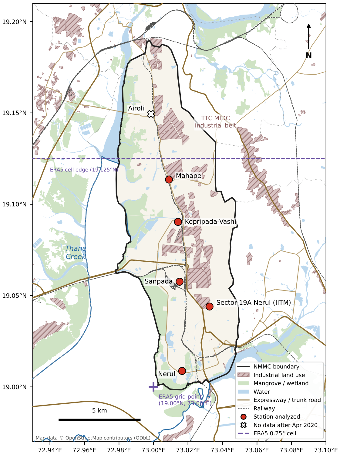
Figure 2.
Monthly mean PM at the five Navi Mumbai stations, 2021–2025. Months with fewer than 15 valid days are not shown. Shading marks the monsoon (June–September); the dotted line is the 24-hour NAAQS. Source: Authors’ estimation.
Figure 2.
Monthly mean PM at the five Navi Mumbai stations, 2021–2025. Months with fewer than 15 valid days are not shown. Shading marks the monsoon (June–September); the dotted line is the 24-hour NAAQS. Source: Authors’ estimation.
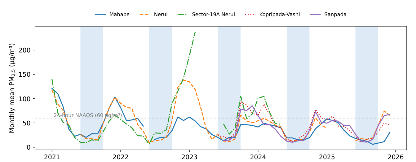
Figure 3.
Daily benzene at Mahape as reported, 2021–2025. Values in runs of three or more identical daily means (including runs of zeros) and non-positive values are removed before estimation. Source: Authors’ estimation.
Figure 3.
Daily benzene at Mahape as reported, 2021–2025. Values in runs of three or more identical daily means (including runs of zeros) and non-positive values are removed before estimation. Source: Authors’ estimation.
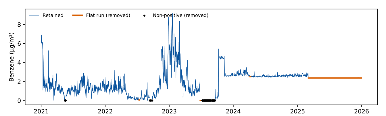
Figure 4.
Median diurnal profiles of pollutants relative to their daily mean, Mahape and Nerul, by season, 2021–2025. Shading: median ERA5 BLH (right axis). O is omitted where fewer than 20 hourly medians are available. Source: Authors’ estimation.
Figure 4.
Median diurnal profiles of pollutants relative to their daily mean, Mahape and Nerul, by season, 2021–2025. Shading: median ERA5 BLH (right axis). O is omitted where fewer than 20 hourly medians are available. Source: Authors’ estimation.
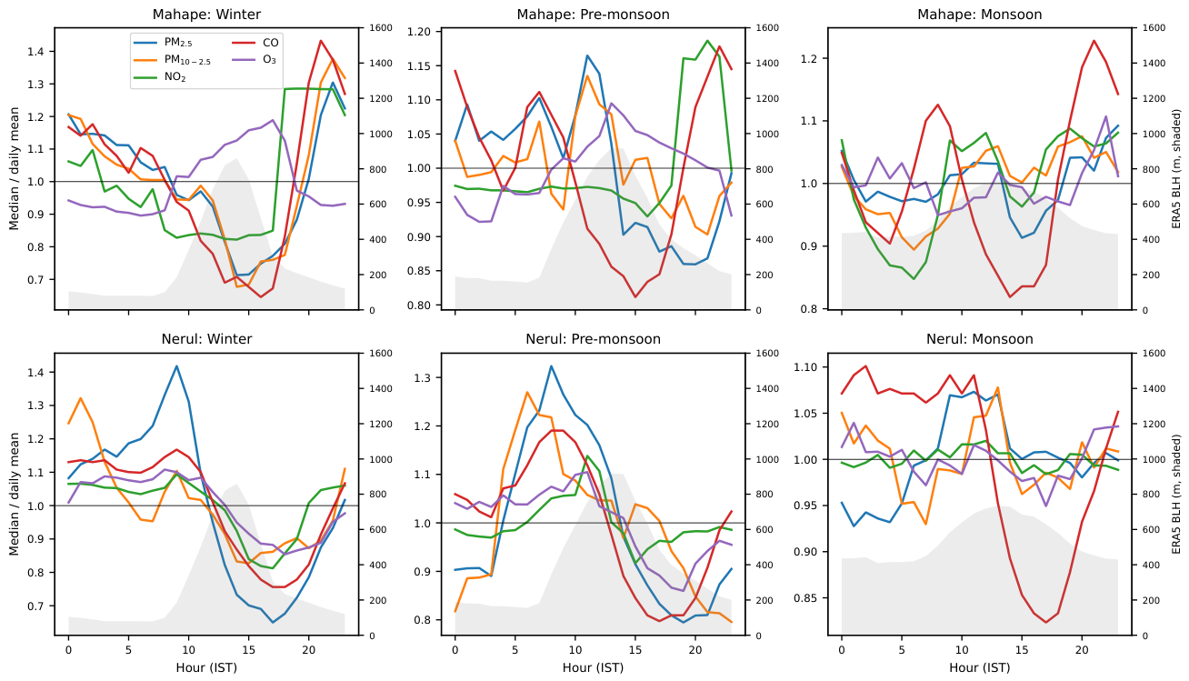
Figure 5.
Median hourly PM on land–sea breeze days and other dry-season days (October–May) at Mahape and Nerul, and the monthly share of breeze days (ERA5 classification), 2021–2025. Raw medians, not adjusted for weather or season. Source: Authors’ estimation.
Figure 5.
Median hourly PM on land–sea breeze days and other dry-season days (October–May) at Mahape and Nerul, and the monthly share of breeze days (ERA5 classification), 2021–2025. Raw medians, not adjusted for weather or season. Source: Authors’ estimation.
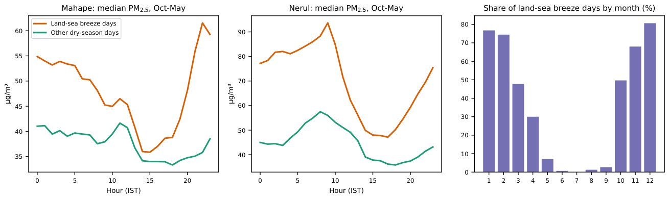
Figure 6.
Station-level results on the map. (a) Mean PM; (b) share of days above the 24-hour NAAQS; (c) own share of the forecast-error variance (FEV) of PM at a horizon h of 10 days; (d,e) same-day percentage effect of a one-SD increase in rainfall and BLH; (f) RMSE of one-day-ahead XGBoost forecasts relative to persistence (negative: XGBoost more accurate). Source: Authors’ estimation; map data © OpenStreetMap contributors (ODbL).
Figure 6.
Station-level results on the map. (a) Mean PM; (b) share of days above the 24-hour NAAQS; (c) own share of the forecast-error variance (FEV) of PM at a horizon h of 10 days; (d,e) same-day percentage effect of a one-SD increase in rainfall and BLH; (f) RMSE of one-day-ahead XGBoost forecasts relative to persistence (negative: XGBoost more accurate). Source: Authors’ estimation; map data © OpenStreetMap contributors (ODbL).
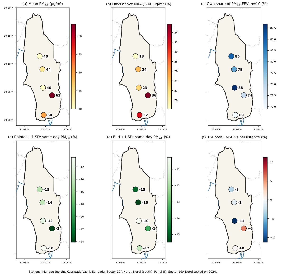
Figure 7.
(a) Stations analyzed, numbered as in panel (b). (b) Correlation of daily log PM for each station pair against the distance between the stations, computed over each pair’s overlapping days; the dashed line is a least-squares fit. Source: Authors’ estimation; map data © OpenStreetMap contributors (ODbL).
Figure 7.
(a) Stations analyzed, numbered as in panel (b). (b) Correlation of daily log PM for each station pair against the distance between the stations, computed over each pair’s overlapping days; the dashed line is a least-squares fit. Source: Authors’ estimation; map data © OpenStreetMap contributors (ODbL).
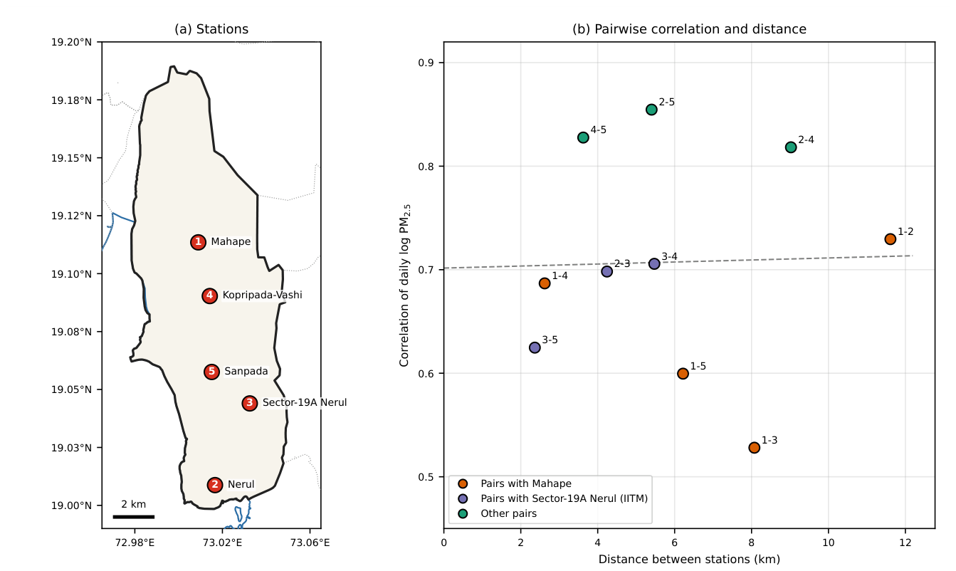
Figure 8.
Observed PM and one-day-ahead forecasts at Mahape, 2025. XGBoost with same-day weather; persistence is the previous day’s value. Shading marks the monsoon. Source: Authors’ estimation.
Figure 8.
Observed PM and one-day-ahead forecasts at Mahape, 2025. XGBoost with same-day weather; persistence is the previous day’s value. Shading marks the monsoon. Source: Authors’ estimation.
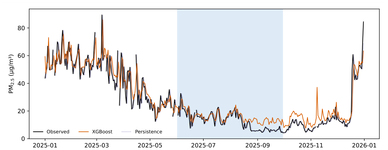
Figure 9.
Share of days with PM above the 24-hour NAAQS on stagnant and other days, 2021–2025. Source: Authors’ estimation.
Figure 9.
Share of days with PM above the 24-hour NAAQS on stagnant and other days, 2021–2025. Source: Authors’ estimation.
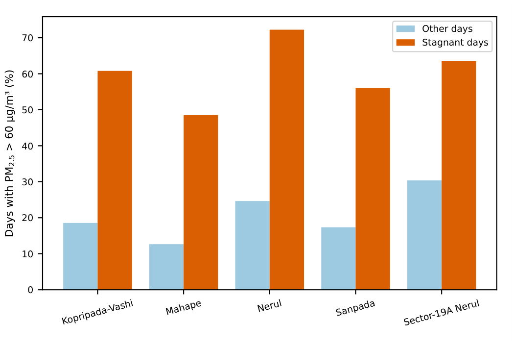

Table 1.
Monitoring stations and daily PM, 2021–2025.
| Station | Operator | PM record | Days | Cov. (%) | Mean | Median | P90 | >60 (%) | Winter | Monsoon | PM |
|---|---|---|---|---|---|---|---|---|---|---|---|
| Mahape | MPCB | Jan 2021–Dec 2025 | 1,735 | 95 | 39.9 | 34.4 | 74.3 | 18 | 64.1 | 18.7 | 79.7 |
| Nerul | MPCB | Jan 2021–Dec 2025 | 1,616 | 88 | 49.9 | 38.6 | 108.0 | 32 | 86.3 | 16.3 | 85.7 |
| Sector-19A Nerul | IITM | Jan 2021–Nov 2024 | 1,100 | 78 | 63.3 | 46.9 | 141.0 | 36 | 110.3 | 24.3 | 51.9 |
| Kopripada-Vashi | MPCB | Jun 2023–Dec 2025 | 917 | 99 | 43.6 | 39.4 | 85.2 | 24 | 64.2 | 19.0 | 51.6 |
| Sanpada | MPCB | Jun 2023–Dec 2025 | 898 | 98 | 40.1 | 34.7 | 80.6 | 23 | 60.1 | 14.9 | 60.4 |
Daily (24-hour) means in µg/m3 after screening (Section 2.2). Cov.: share of days with a valid PM2.5 value between the first and last valid day. >60: share of valid days above the 24-hour NAAQS of 60 µg/m3. Winter: December–February; Monsoon: June--September. PM10− 2.5: mean coarse fraction. Airoli (MPCB) is excluded: its hourly and daily repository files for 2021–2025 contain no measurements (last valid readings 9 April 2020). Source: Authors’ estimation.
Table 2.
Station locations and surroundings.
| Station | Operator | PM analyzer | Lat. (N) | Lon. (E) | Creek shoreline (km) | Industrial land (km) | Major road (km) | In ERA5 cell | Status |
|---|---|---|---|---|---|---|---|---|---|
| Mahape | MPCB | n.p. | 19.1135 | 73.0090 | 3.2 | 0.04 | 0.01 | yes | Analyzed |
| Airoli | MPCB | n.p. | 19.1494 | 72.9986 | 3.6 | 0.24 | 0.14 | no | No data after Apr 2020 |
| Kopripada-Vashi | MPCB | n.p. | 19.0903 | 73.0142 | 3.0 | 0.40 | 0.12 | yes | Analyzed |
| Sanpada | MPCB | n.p. | 19.0576 | 73.0151 | 2.1 | 0.50 | 0.43 | yes | Analyzed |
| Sector-19A Nerul | IITM | n.p. | 19.0440 | 73.0325 | 3.4 | 0.04 | 0.46 | yes | Analyzed |
| Nerul | MPCB | n.p. | 19.0088 | 73.0166 | 0.8 | 1.22 | 0.14 | yes | Analyzed |
Distances are to the nearest OpenStreetMap coastline segment (Thane Creek), industrial land-use polygon and motorway, trunk or primary road, computed on a local planar projection. “In ERA5 cell”: inside the 0.25° cell centered on the ERA5 grid point (19.00°N, 73.00°E) used for all meteorological variables. PM analyzer: make and measurement principle of the particulate monitor; n.p.: not published in the CPCB repository or station metadata. Map data © OpenStreetMap contributors (ODbL).
Source: Authors' estimation.
Table 3.
Effect bounds and equivalence tests for lagged co-pollutants in the PM equation.
| Lagged variable | Effect (%/SD) | 95% CI | 90% CI | TOST p | Holm p | BH p |
|---|---|---|---|---|---|---|
| Panel A. Mahape, VARX(1) with eight pollutants | ||||||
| PM | -2.2 | [-4.9, +0.6] | [-4.4, +0.1] | 0.030 | 0.503 | 0.213 |
| NO | +0.7 | [-1.7, +3.1] | [-1.4, +2.7] | <0.001 | 0.993 | 0.589 |
| CO | -1.7 | [-3.6, +0.3] | [-3.3, +0.0] | <0.001 | 0.503 | 0.213 |
| SO | +2.4 | [-0.2, +5.0] | [+0.2, +4.6] | 0.026 | 0.439 | 0.213 |
| O | +3.9 | [+1.8, +6.0] | [+2.1, +5.6] | 0.146 | 0.002 | 0.002 |
| NH | -1.2 | [-3.1, +0.8] | [-2.8, +0.5] | <0.001 | 0.721 | 0.336 |
| Benzene | +0.8 | [-1.6, +3.3] | [-1.2, +2.9] | <0.001 | 0.993 | 0.579 |
| All seven jointly | p <0.001 | partial 0.021 | ||||
| Panel B. All stations, VARX(1) with six pollutants: pollutants shown equivalent to zero (TOST ) and joint block | ||||||
| Mahape | NO, CO, SO, O | 0.003 | 0.018 | |||
| Nerul | NO, O | 0.058 | 0.015 | |||
| Sector-19A Nerul | NO | 0.072 | 0.017 | |||
| Kopripada-Vashi | PM, NO, CO, SO | 0.414 | 0.007 | |||
| Sanpada | NO, SO, O | 0.342 | 0.009 | |||
Effect: percentage change in next-day PM2.5 after a one-standard-deviation increase in the log of the lagged pollutant, holding the other regressors fixed. TOST: two one-sided tests of the null that the effect lies outside ±5% per SD; p < 0.05 establishes that the effect is smaller than 5% in absolute value (the 90% CI lies inside the margin). Holm: family-wise adjustment; BH: Benjamini
and Hochberg [61] false-discovery-rate adjustment of the Granger p-values. Partial R2: share of the residual variance of the restricted model (without co-pollutant lags) explained by adding them. In Panel B the last three columns give the joint F-test, its p-value and the partial R2. Source: Authors’ estimation.
Table 4.
What the controls and the coarse fraction change: Granger p-values in the PM equation, Mahape.
Table 4.
What the controls and the coarse fraction change: Granger p-values in the PM equation, Mahape.
| (A) | (B) | (C) | (D) | |
|---|---|---|---|---|
| Granger p-value for the lagged variable | ||||
| PM (A only) | 0.384 | – | – | – |
| PM | – | 0.274 | 0.747 | 0.122 |
| NO | 0.015 | 0.014 | 0.670 | 0.589 |
| CO | 0.360 | 0.340 | 0.224 | 0.101 |
| SO | 0.039 | 0.036 | 0.130 | 0.073 |
| O | 0.002 | 0.002 | <0.001 | <0.001 |
| NH | 0.087 | 0.099 | 0.125 | 0.240 |
| Benzene | 0.888 | 0.873 | 0.631 | 0.496 |
| Fit | ||||
| , PM equation | 0.808 | 0.808 | 0.832 | 0.855 |
| Own share of GFEVD, (%) | 51.2 | 66.2 | 70.9 | 75.2 |
All columns use one lag and the same days. (A) PM in place of the coarse fraction, no exogenous controls; (B) coarse fraction PM, no controls; (C) adds month, day-of-week, year, lockdown and Diwali effects; (D) adds same-day and lagged ERA5 rainfall, boundary-layer height, temperature, humidity and wind components (the main specification). Unadjusted p-values of HC1 Wald tests. Source: Authors’ estimation.
Table 5.
Weather and calendar terms in the PM equation, Mahape.
| Same day | Lag 1 | ||||
|---|---|---|---|---|---|
| Meteorology (ERA5) | |||||
| Rainfall, log(1+mm) | -0.112 (0.018) | 0.043 (0.022) | -14.1 | -3.6 | -1.4 |
| Boundary-layer height, log m | -0.415 (0.075) | 0.294 (0.058) | -15.6 | 0.5 | 0.6 |
| Temperature | 0.069 (0.021) | -0.073 (0.021) | 13.5 | -5.2 | -2.2 |
| Relative humidity | 0.004 (0.003) | -0.003 (0.003) | 4.0 | -1.1 | -0.3 |
| Zonal wind u (westerly +) | 0.042 (0.016) | -0.030 (0.014) | 7.2 | -0.6 | -0.8 |
| Meridional wind v (southerly +) | -0.008 (0.012) | 0.003 (0.011) | -1.8 | -1.0 | -0.4 |
| Calendar events | |||||
| Lockdown, Apr–Jun 2021 | -0.134 (0.055) | ||||
| Diwali window (±2 days) | 0.130 (0.059) | ||||
| Block tests | |||||
| Joint test: Meteorology (12 terms) | <0.001 | ||||
| Joint test: Month effects | 0.268 | ||||
| Joint test: Day-of-week effects | 0.004 | ||||
| Joint test: Year effects | <0.001 | ||||
| Joint test: Lagged co-pollutants (all) | <0.001 | ||||
Columns 2–3: coefficients (HC1 standard errors) in the log PM equation of the VARX(1). Columns 4–6: dynamic multipliers, the percentage response of PM at horizon h to a one-standard-deviation increase in the weather variable on day 0, propagated through the estimated VARX dynamics. Temperature in C, humidity in %, wind in m/s. Source: Authors’ estimation.
Table 6.
Hourly VARX: Granger tests for co-pollutants in the PM equation.
| Lagged variable | Wald F | p | Holm p | Lag sum (SE) | GFEVD, 24 h (%) |
|---|---|---|---|---|---|
| Mahape: 24 lags, T = 12,842 hours; own-lag sum 0.957; own GFEVD at 24 h 76.4%; Ljung–Box p = 0.12 | |||||
| PM | <0.001 | <0.001 | -0.021 (0.006) | 14.6 | |
| NO | <0.001 | <0.001 | -0.007 (0.005) | 1.1 | |
| CO | <0.001 | <0.001 | -0.003 (0.005) | 7.3 | |
| O | <0.001 | <0.001 | 0.004 (0.005) | 0.6 | |
| All co-pollutants jointly | <0.001 | ||||
| Nerul: 30 lags, T = 15,992 hours; own-lag sum 0.954; own GFEVD at 24 h 78.2%; Ljung–Box p = 0.92 | |||||
| PM | <0.001 | <0.001 | -0.009 (0.007) | 5.9 | |
| NO | <0.001 | <0.001 | 0.006 (0.004) | 1.8 | |
| CO | <0.001 | <0.001 | -0.018 (0.007) | 14.1 | |
| All co-pollutants jointly | <0.001 | ||||
Hourly VARX in log concentrations with same-hour and lagged ERA5 weather and hour-of-day, day-of-week, month, year, lockdown and Diwali terms; hours enter only if all lags are observed. Lag order: at Nerul the BIC choice over 1–48 hours (30); at Mahape BIC selects 6 hours but the residuals remain autocorrelated (Ljung–Box ), so the smallest order with white residuals (24) is used. Lag sum: sum of the lag coefficients (HC1 standard error). GFEVD: share of the 24-hour-ahead forecast-error variance of PM. O is omitted at Nerul, where it is missing for most hours. Source: Authors’ estimation.
Table 7.
What the city-wide daily effects contain.
| Explanatory variables for the date effects | Terms | Share of total variance | |
|---|---|---|---|
| Weather (ERA5, same day and lag 1) | 12 | 0.733 | 0.569 |
| Weather incl. nonlinear terms | 16 | 0.744 | 0.577 |
| Calendar only (month, day of week, year, events) | 23 | 0.713 | 0.553 |
| Weather + calendar | 35 | 0.794 | 0.616 |
| Weather incl. nonlinear + calendar | 39 | 0.797 | 0.618 |
| XGBoost, weather + calendar (out-of-sample, time-ordered CV) | 18 | 0.662 | 0.513 |
Date effects are estimated from a regression of log PM on station and date fixed effects across the five stations (6266 station-days); together these explain 0.785 of the variance and station effects alone 0.010. The date effects are regressed on the listed variables with weights equal to the number of stations reporting that day. Share of total variance: times the share of the variance of log PM attributable to date effects. The XGBoost row is an out-of-sample from five-fold time-ordered cross-validation. Source: Authors’ estimation.
Table 8.
One-day-ahead PM forecasts, Mahape, 2025.
| Model | RMSE | MAE | Bias | POD | FAR | DM vs XGBoost (p) | |
|---|---|---|---|---|---|---|---|
| Weather on target day; all forecastable days (N = 346) | |||||||
| XGBoost | 6.84 | 5.15 | 0.884 | 2.22 | 0.44 | 0.40 | – |
| Persistence | 7.07 | 4.43 | 0.876 | -0.32 | 0.37 | 0.57 | -0.62 (0.537) |
| Monthly climatology | 21.91 | 16.84 | -0.189 | 15.88 | 0.78 | 0.76 | -4.82 (<0.001) |
| Weather on target day; days with complete inputs for all models (N = 176) | |||||||
| XGBoost | 5.76 | 4.71 | 0.926 | 2.67 | 0.50 | 0.38 | – |
| Persistence | 4.82 | 2.98 | 0.949 | -0.38 | 0.50 | 0.43 | 2.17 (0.031) |
| Monthly climatology | 24.45 | 19.94 | -0.327 | 19.34 | 1.00 | 0.67 | -4.50 (<0.001) |
| Linear ARX (same inputs) | 6.37 | 5.15 | 0.910 | 3.56 | 0.75 | 0.50 | -1.49 (0.139) |
| VARX(1) PM equation | 5.01 | 3.60 | 0.944 | 2.57 | 0.81 | 0.41 | 1.49 (0.138) |
| Lagged weather only; all forecastable days (N = 346) | |||||||
| XGBoost | 8.06 | 6.57 | 0.839 | 3.46 | 0.33 | 0.44 | – |
| Persistence | 7.07 | 4.43 | 0.876 | -0.32 | 0.37 | 0.57 | 1.85 (0.065) |
| Monthly climatology | 21.91 | 16.84 | -0.189 | 15.88 | 0.78 | 0.76 | -4.79 (<0.001) |
| Lagged weather only; days with complete inputs for all models (N = 176) | |||||||
| XGBoost | 7.69 | 6.70 | 0.869 | 4.55 | 0.31 | 0.44 | – |
| Persistence | 4.82 | 2.98 | 0.949 | -0.38 | 0.50 | 0.43 | 4.41 (<0.001) |
| Monthly climatology | 24.45 | 19.94 | -0.327 | 19.34 | 1.00 | 0.67 | -4.42 (<0.001) |
| Linear ARX (same inputs) | 6.26 | 5.20 | 0.913 | 3.57 | 0.62 | 0.52 | 3.31 (0.001) |
| VARX(1) PM equation | 5.21 | 3.96 | 0.940 | 2.73 | 0.69 | 0.48 | 4.07 (<0.001) |
Out-of-sample forecasts for 2025 with every model re-estimated at the start of each month on all earlier data (expanding window). Errors in µg/m; within each panel all models are evaluated on the same days. The linear models need every input to be observed, so the second panel of each setting is restricted to those days. Bias: mean forecast minus observation. POD and FAR: probability of detection and false-alarm ratio for days above 60 µg/m. DM: Diebold and Mariano [45] statistic with the Harvey et al. [46] correction on the loss differential (XGBoost minus benchmark squared error); a negative value means XGBoost has smaller errors than the benchmark, a positive value that it has larger errors. Inputs: lags 1, 2, 3 and 7 of the six pollutants, ERA5 weather (same day and lag 1, or lag 1 only) and calendar terms; no same-day pollutant enters. Source: Authors’ estimation.
Table 9.
A stagnation index as a warning trigger for days above 60 µg/m.
| Warning rule | Mahape | Nerul | Sector-19A | Kopripada | Sanpada | Pooled |
|---|---|---|---|---|---|---|
| Panel A. Probability of detection / false-alarm ratio | ||||||
| Stagnation index (forecast weather) | 0.59 / 0.67 | 0.38 / 0.30 | 0.25 / 0.22 | 0.42 / 0.60 | 0.38 / 0.40 | 0.37 / 0.48 |
| Stagnation index (yesterday’s weather) | 0.48 / 0.72 | 0.30 / 0.42 | 0.23 / 0.32 | 0.40 / 0.62 | 0.37 / 0.39 | 0.33 / 0.52 |
| Persistence (yesterday > 60) | 0.37 / 0.57 | 0.80 / 0.18 | 0.83 / 0.18 | 0.58 / 0.42 | 0.65 / 0.33 | 0.69 / 0.30 |
| Stagnation or persistence | 0.70 / 0.68 | 0.88 / 0.27 | 0.83 / 0.22 | 0.76 / 0.56 | 0.80 / 0.40 | 0.81 / 0.42 |
| Winter season (Nov-Feb) | 0.78 / 0.82 | 0.80 / 0.48 | 0.66 / 0.11 | 0.80 / 0.67 | 0.64 / 0.55 | 0.71 / 0.57 |
| XGBoost forecast > 60 | 0.44 / 0.40 | 0.86 / 0.25 | 0.86 / 0.17 | 0.64 / 0.45 | 0.67 / 0.26 | 0.73 / 0.28 |
| Panel B. Peirce skill score [90% block-bootstrap interval] | ||||||
| Stagnation index (forecast weather) | 0.49 [0.28, 0.62] | 0.33 [0.15, 0.48] | 0.17 [0.07, 0.30] | 0.31 [0.16, 0.46] | 0.30 [0.19, 0.43] | 0.28 [0.23, 0.34] |
| Stagnation index (yesterday’s weather) | 0.38 [0.24, 0.49] | 0.23 [0.08, 0.37] | 0.11 [0.01, 0.25] | 0.29 [0.16, 0.45] | 0.29 [0.19, 0.41] | 0.24 [0.19, 0.30] |
| Persistence (yesterday > 60) | 0.33 [0.14, 0.46] | 0.75 [0.61, 0.84] | 0.63 [0.50, 0.76] | 0.51 [0.36, 0.64] | 0.55 [0.44, 0.65] | 0.62 [0.55, 0.68] |
| Stagnation or persistence | 0.58 [0.35, 0.70] | 0.78 [0.68, 0.86] | 0.58 [0.43, 0.71] | 0.60 [0.48, 0.71] | 0.63 [0.52, 0.72] | 0.66 [0.60, 0.71] |
| Winter season (Nov-Feb) | 0.48 [0.24, 0.68] | 0.58 [0.33, 0.78] | 0.57 [0.40, 0.75] | 0.54 [0.37, 0.69] | 0.40 [0.21, 0.55] | 0.46 [0.37, 0.55] |
| XGBoost forecast > 60 | 0.42 [0.23, 0.57] | 0.78 [0.63, 0.89] | 0.66 [0.53, 0.77] | 0.55 [0.39, 0.71] | 0.59 [0.47, 0.70] | 0.65 [0.59, 0.72] |
| Panel C. Discrimination and base rates | ||||||
| Ventilation coefficient, AUC | 0.79 | 0.88 | 0.77 | 0.75 | 0.83 | – |
| Events (test year) | 27 | 50 | 83 | 50 | 84 | 294 |
| Exceedance frequency, stagnant / other days (%) | 48 / 13 | 72 / 25 | 63 / 30 | 61 / 19 | 56 / 17 | – |
Out-of-sample forecasts for 2025 with every model re-estimated at the start of each month on all earlier data (expanding window). Errors in \textmu g/m3; within each panel all models are evaluated on the same days. The linear models need every input to be observed, so the second panel of each setting is restricted to those days. Bias: mean forecast minus observation. POD and FAR: probability of detection and false-alarm ratio for days above 60 \textmu g/m3. DM: Diebold and Mariano [45] statistic with the Harvey et al. [46] correction on the loss differential (XGBoost minus benchmark squared error); a negative value means XGBoost has smaller errors than the benchmark, a positive value that it has larger errors. Inputs: lags 1, 2, 3 and 7 of the six pollutants, ERA5 weather (same day and lag 1, or lag 1 only) and calendar terms; no same-day pollutant enters.
Source: Authors' estimation.
Disclaimer/Publisher’s Note: The statements, opinions and data contained in all publications are solely those of the individual author(s) and contributor(s) and not of MDPI and/or the editor(s). MDPI and/or the editor(s) disclaim responsibility for any injury to people or property resulting from any ideas, methods, instructions or products referred to in the content. |
© 2026 by the authors. Licensee MDPI, Basel, Switzerland. This article is an open access article distributed under the terms and conditions of the Creative Commons Attribution (CC BY) license.
Copyright: This open access article is published under a Creative Commons CC BY 4.0 license, which permit the free download, distribution, and reuse, provided that the author and preprint are cited in any reuse.